KIAS-P20063

5D BPS Quivers and KK Towers

Zhihao Duan, Dongwook Ghim, and Piljin Yi

School of Physics, Korea Institute for Advanced Study, Seoul 02455, Korea

We explore BPS quivers for $D=5$ theories, compactified on a circle and geometrically engineered over local Calabi-Yau 3-folds, for which many of known machineries leading to (refined) indices fail due to the fine-tuning of the superpotential. For Abelian quivers, the counting reduces to a geometric one, but the technically challenging $L^{2}$ cohomology proved to be essential for sensible BPS spectra. We offer a mathematical theorem to remedy the difficulty, but for non-Abelian quivers, the cohomology approach itself fails because the relevant wavefunctions are inherently gauge-theoretical. For the Cartan part of gauge multiplets, which suffers no wall-crossing, we resort to the D0 picture and reconstruct entire KK towers. We also perform numerical checks using a multi-center Coulombic routine, with a simple hypothesis on the quiver invariants, and extend this to electric BPS states in the weak coupling chamber. We close with a comment on known Donaldson-Thomas invariants and on how $L^{2}$ index might be read off from these.

1 $D=5$ BPS Quiver

Five-dimensional gauge theories with eight supercharges [1] can be constructed via “compactifying” M-theory on local Calabi-Yau 3-folds [2, 3]. One can hone in for degrees of freedom localized at the bottom of such asymptotically conical “internal” manifolds, while ignoring the bulk gravity. This way of realizing supersymmetric theories via local Calabi-Yau’s is broadly called geometric engineering [4, 5]. The gauge multiplet comes with a single real adjoint scalar, and this renders the dynamics along the Coulombic degrees of freedom a lot simpler and qualitatively different from its $D=4$ counterpart, namely the Seiberg-Witten theories [6]. Despite such an apparent simplification, the $D=5$ BPS spectra have been studied less vigorously.

One curious aspect of $D=5$ BPS spectra, relative to $D=4$, is the absence of the wall-crossing. One rationale behind this is that the central charges of point-like objects are now real, so the well-known mechanism behind the wall-crossing is no longer viable. What remains unclear though is exactly how this cross-over between $D=4$ and $D=5$ should be understood from the dynamics of these special objects themselves.

It is well-known that the dynamics of BPS objects in $D=4$ is described by quiver quantum mechanics, well-known from type IIB perspective [8] but also derived directly from the Seiberg-Witten field theory near a wall of marginal stability [9]. The rank of each node is the number of the respective building blocks, such as fundamental monopoles and dyons. The number of bifundamental chirals between a pair of quiver nodes is determined by the Schwinger product between the respective building blocks. The wall-crossing is captured by the discontinuity [10] of the refined Witten index [11] of such quantum mechanics in the parameter space of the Fayet-Iliopoulos (FI) constants, which are in turn related to the phases of these primitive dyons.

One issue with uplifting this picture to $D=5$ is that the primitive BPS objects, corresponding to each node of $D=4$ BPS quiver, uplift to objects with one spatial dimension, such as BPS monopole strings; Does this mean that the quiver quantum mechanics uplifts to $d=2$ quiver linear sigma model?

On the surface, this might sound attractive since the elliptic genus is well-known to be safe from D-term wall-crossing [12]. However, its computation relies on $T^{2}$, which means that $d=2$ GLSM’s suffer no such wall-crossing even if compactified on a circle; if $D=5$ BPS objects were governed by $d=2$ linear sigma models, they would not have experienced the wall-crossing even on $\mathbb{S}^{1}\times\mathbb{R}^{3+1}$ either. It is by now well-known how the elliptic genus, with no wall-crossing on the D-term parameter space, becomes piece-wise constant only in the strict limit of $d=1$ [10], while BPS states of $D=5$ theories compactified on a circle, should experience wall-crossing, since their central charges are still complex. So the uplift of $D=4$ BPS quiver to $D=5$ cannot be understood as the simple dimensional uplift of its $d=1$ quiver description.

One can also see why this naive uplift of $d=1$ GLSM to $d=2$ is a bad idea from the simplest example of $D=4$ BPS quiver for pure $SU(2)$ Seiberg-Witten theory, namely a Kronecker quiver with intersection number 2 [8]. The two nodes represent monopoles and dyons, with charges $(0,1)$ and $(2,-1)$, respectively. In the semi-classical picture these are a solitonic monopole and a solitonic anti-monopole bound with a single vector meson. In going over to $D=5$, the magnetic part uplifts to strings while the charged vector multiplet remains as a particle. What should be noted here is that the two objects are of opposite magnetic charge, and thus of opposite orientations; the usual non-relativistic approximation to extract the low energy dynamics of such solitons no longer works.

In fact, viewing the whole situation from M-theory, the relevant objects for magnetic sector are M5 branes wrapping 4-cycles in the Calabi-Yau, and as such the natural theory on these string-like objects are of $(0,4)$ supersymmetry [13, 14], rather than $(2,2)$ which would be naively suggested by the $d=1$ quiver theories that governed $D=4$ BPS particle dynamics.

Recently, on the other hand, an interesting middle ground was offered in Ref. [15]. The authors asked what would be the useful low energy dynamics if one compactifies $D=5$ gauge theory on a circle $\mathbb{S}^{1}$ and considers particle-like states, relative to the remaining noncompact part of the spacetime, $\mathbb{R}^{3+1}$; Although the monopole and the dyon would be still string-like, one considers only those configurations where these strings are wrapped along $\mathbb{S}^{1}$. These can wiggle along the circle, but such wiggles can be attributed to Kaluza-Klein (KK) momenta, to be treated as separate degrees of freedom. The latter approach allows dynamics of $D=5$ BPS states to be described yet again by some $d=1$ quiver theory, with more elementary nodes relative to that of purely $D=4$ BPS states. The downside is that the decompactification limit $\mathbb{S}^{1}\rightarrow\mathbb{R}^{1}$ requires an infinite sum over KK charges, so the question of exactly how the wall-crossing disappears in strict $D=5$ limit becomes a little remote.

$D=4$ BPS quiver, e.g., for pure gauge theory of rank $r$ simple gauge group, comes with $2r$ primitive nodes typically. The magnetic part of these $2r$ dyons is labeled by “simple” dual roots. Upon going up one higher dimension with $\mathbb{S}^{1}$, the Dynkin diagram naturally uplifts to the affine Dynkin diagram, so we can expect two more nodes whose magnetic charges belong to the $(r+1)$-th node of the affine Dynkin diagram. $D=5$ implies two additional types of charges as well, namely the KK charge along $\mathbb{S}^{1}$ and the instanton-soliton charge on $\mathbb{S}^{1}\times\mathbb{R}^{3}$, which should also enter these additional nodes as well. For example, with the pure $SU(2)$ supersymmetric gauge theory, one finds a cyclic 4-node BPS quiver with the four neighboring intersection numbers all equal to 2.

How does one figure out the quiver theory, given a $D=5$ gauge theory? It turns out that this question has a more systematic answer than its $D=4$ counterpart, thanks to the presence of the KK modes, i.e., D0 branes. D0 probe theory for the local Calabi-Yau would be a quiver quantum mechanics, whose individual nodes correspond to fractional branes. These fractional branes, M2 branes wrapping 2-cycles and M5 branes wrapping 4-cycles times $\mathbb{S}^{1}$, offer basic building blocks for BPS states of $D=5$ theory on $\mathbb{S}^{1}$, so the D0 probe theory can be naturally adopted as $D=5$ BPS quiver [15].

In the context of type IIB theory, on the other hand, systematic construction of the probe D3 theory for such local Calabi-Yau has been pursued since late 90’s, most notably by Feng, He, and Hanany [16]. The construction in terms of the $d=4$ gauge theory, with four supercharges, is by now well-established, with various techniques such as Brane Tiling [17, 18, 19], for toric Calabi-Yau. As such, all one has to do is to import this technology for D0’s [15].

1.1 Orbifolds

Calabi-Yau’s obtained from orbifolding $\mathbb{C}^{3}$ by a discrete Abelian subgroup $\Gamma$ of $SU(3)$ offer the simplest examples [20, 21]. For $n$ D0 probes, one starts with $n\times|\Gamma|$ many D0’s and orbifolding will lead to a quiver theory with $|\Gamma|$ many nodes, each with gauge group $U(n)$. One can choose to assign different ranks to the nodes, which corresponds to adding fractional branes localized near the orbifold point. The partial resolutions of these orbifolds are also known to lead to other toric examples [22, 16], to which we will turn later in the next subsection.

One of the simplest examples of local Calabi-Yau’s is local $\mathbb{P}^{2}$ with the asymptotic cone $\mathbb{C}^{3}/\mathbb{Z}_{3}$. Although this does not produce a Seiberg-Witten gauge theory, it does offer the $D=5$ BPS quiver in its simplest and non-trivial form. The probe theory with $n$ D0 branes starts by projecting the maximally supersymmetric $U(3n)$ Yang-Mills by $\mathbb{Z}_{3}$ which acts on three complex coordinates by multiplying $(w,w,w^{-2})$ with $w$ a 3rd root of unity. The resulting quiver is a cyclic triangle quiver with three bifundamentals for each pair of nodes.

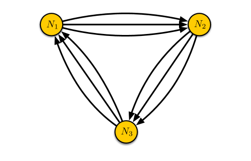
Figure 1: The quiver diagram of $\mathbb{C}^{3}/\mathbb{Z}_{3}$ orbifold theory.

From the viewpoint of the original D0 theory prior to the orbifolding, these bifundamental chirals can be embedded into three $U(3n)$ complex adjoints as

$$X=\left(\begin{array}[]{ccc}0&x_{12}&0\\ 0&0&x_{23}\\ x_{31}&0&0\end{array}\right)\ ,\;Y=\left(\begin{array}[]{ccc}0&y_{12}&0\\ 0&0&y_{23}\\ y_{31}&0&0\end{array}\right)\ ,\;Z=\left(\begin{array}[]{ccc}0&z_{12}&0\\ 0&0&z_{23}\\ z_{31}&0&0\end{array}\right)\,$$ (1.10)

which survive the projection

$$x_{ij}=w^{1+i-j}x_{ij}\ ,\qquad y_{ij}=w^{1+i-j}y_{ij}\ ,\qquad z_{ij}=w^{1+i-j}z_{ij}$$ (1.11)

with $w=e^{2\pi i/3}$. The subscripts denote the pair of gauge nodes, with respect to which these chirals are bifundamental. Note that the superpotential is not generic but must descend from the cubic superpotential of the maximally supersymmetric $U(3n)$ theory, i.e.,

$$W=\frac{1}{3}{\rm tr}\left(X[Y,Z]\right)=\frac{1}{3}{\rm tr}\left(x_{12}y_{23}z_{31}-x_{12}z_{23}y_{31}+\cdots\right)$$ (1.12)

where the ellipsis denotes the cyclic permutations of $x,y,z$. In fact, this fine-tuned superpotential is a hallmark of local Calabi-Yau, and the precise construction of $W$ has been offered through the brane tiling machinery [17, 18, 19].

The transition to smooth local $\mathbb{P}^{2}$, from the singular orbifold, is naturally described by turning on FI constants on these three $U(n)$ nodes, which corresponds to moving out into the Coulombic moduli space of the $D=5$ theory. In a sense this is the simplest prototype of $D=5$ BPS quivers, associated with the so-called $E_{0}$ theory [2].

More elaborate examples can be found from the orbifold $\mathbb{C}^{3}/\mathbb{Z}_{p}\times\mathbb{Z}_{p}$. One projects $U(p^{2}n)$ theory via

$$x_{ij;kl}=w^{1+i-k}x_{ij;kl}\ ,\qquad y_{ij;kl}=w^{i-k}y_{ij;kl}\ ,\qquad z_{ij;kl}=w^{-1+i-k}z_{ij;kl}\ ,$$ (1.13)

and

$$x_{ij;kl}=w^{j-l}x_{ij;kl}\ ,\qquad y_{ij;kl}=w^{1+j-l}y_{ij;kl}\ ,\qquad z_{ij;kl}=w^{-1+j-l}z_{ij;kl}\ ,$$ (1.14)

with $w=e^{2\pi i/p}$ and the labels valued in $\mathbb{Z}_{p}$. The surviving blocks are,

$$x_{ij;i+1,j}\ ,\qquad y_{ij;i,j+1}\ ,\qquad z_{i+1,j+1;ij}\ ,$$ (1.15)

which are $3p^{2}$ bifundamentals that connect $p^{2}$ $U(n)$’s.

For example, the theory of $n$ D0-branes that probes $\mathbb{C}^{3}/\mathbb{Z}_{2}\times\mathbb{Z}_{2}$ comes with four nodes and twelve $U(n)$ complex bifundamental chirals. Relabeling

$$11\rightarrow 1\ ,\quad 12\rightarrow 2\ ,\quad 21\rightarrow 3\ ,\quad 22\rightarrow 4\ ,$$ (1.16)

the bifundamentals can be embedded into the complex adjoint chirals of $U(2^{2}n)$, e.g.,

$$X=\left(\begin{array}[]{cccc}0&0&x_{13}&0\\ 0&0&0&x_{24}\\ x_{31}&0&0&0\\ 0&x_{42}&0&0\end{array}\right),\;$$ (1.21)

and similarly $Y$ and $Z$ have surviving components, respectively, $(y_{12},y_{21},y_{34},y_{43})$ and $(z_{14},z_{23},z_{32},z_{41})$.

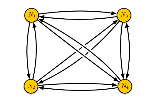
Figure 2: The quiver diagram of $\mathbb{C}^{3}/\mathbb{Z}_{2}\times\mathbb{Z}_{2}$ orbifold theory.

One can see that for every pair of nodes, there are two bifundamental chirals of mutually conjugate gauge representations. Again turning on FI parameters resolves the orbifold singularity. The superpotential is cubic;

$$W=\frac{1}{2^{2}}{\rm tr}\left(X[Y,Z]\right)=\frac{1}{4}{\rm tr}\left(x_{13}y_{34}z_{41}-x_{13}z_{32}y_{21}+\cdots\right)\ ,$$ (1.22)

where the rest of the terms can be constructed by chasing the subscript through the surviving block’s of $X,Y,Z$, with the sign determined by the parity of the permutation of $x,y,z$. Extension of this to $\mathbb{Z}_{p}\times\mathbb{Z}_{p}$ is straightforward. The relabeling of $ij$ for $p>2$,

$$ij\rightarrow(i-1)p+j$$ (1.23)

embeds three sets of the $p^{2}$ bifundamental chirals into three $U(p^{2}n)$ complex adjoint chirals, $X,Y,Z$, respectively, and $W={\rm tr}\left(X[Y,Z]\right)/p^{2}$ contains total $2p^{2}$ monomials, half of which have $1/p^{2}$ and the other half $-1/p^{2}$ as the coefficient.

A special subsector of this orbifold dynamics emerges when we force all the surviving blocks to take values of three common $n\times n$ matrices, $x_{*},y_{*},z_{*}$. The superpotential will collapse to a single cubic commutator potential,

$$W\rightarrow{\rm tr}\left(x_{*}[y_{*},z_{*}]\right)\ ,$$ (1.24)

and the three chirals are each complex adjoint relative to the “diagonal” $U(n)_{*}$ which rotates $U(n)$’s sitting at nodes all simultaneously. This $U(n)_{*}$ together with $x_{*},y_{*},z_{*}$ defines maximally supersymmetric $U(n)$ Yang-Mills theory. Furthermore, the overall $U(1)$ and trace parts of these three complex chirals decouple from the rest of $U(n)_{*}$ theory, and leave behind a maximally supersymmetric $SU(n)$ Yang-Mills. Let us call the latter $SU(n)_{*}$ theory.

This $SU(n)_{*}$ theory has a clear interpretation as the local and relative dynamics of $n$ D0-branes. When D0’s are clustered near each other and sitting at a generic point of the Calabi-Yau, they will see the spacetime locally as $\mathbb{R}^{10}$ unless they are at the top of a singular point; So long as the mutual distances between D0’s are sufficiently small, the dynamics among them would be controlled by the flat space D0 theory. This local dynamics $SU(n)_{*}$ will prove to be a key to obtaining the Kaluza-Klein towers due to $\mathbb{S}^{1}$.

1.2 Partial Resolution of Orbifolds

More examples of local toric Calabi-Yau’s and the accompanying $D=5$ BPS quiver can be found by starting with an orbifold and resolving the singularity partially [22, 16]. This procedure is called “Higgsing” since the resolution involves turning on FI constants partially such that some bifundamental chirals acquire vacuum expectation values.

Among various Calabi-Yau 3-folds which geometrically engineer $D=5$ gauge theory, we introduce two classes of geometry, known as the $Y^{p,q}$ and $X^{p,q}$ families [23, 24, 25, 26], named after the Sasaki-Einstein 5-manifold which occupies their angular direction. We first discuss the former, of which $p=2,q=0$ case ($Y^{2,0}$) is particularly known as local $\mathbb{F}_{0}$ surface, and the latter will be discussed shortly.

$Y^{p,q}$ family and local $\mathbb{F}_{0}$ geometry

Given two non-negative integers $p$ and $q$ such that $p>q\geq 0\,,$ a Calabi-Yau 3-fold $Y^{p,q}$ describes a fibration of the ALE space of $A_{p-1}$ type over $\mathbb{P}^{1}$. It geometrically engineers $D=5$ ${\cal N}=1$ $SU(p)_{q}$ gauge theory [26]. The toric diagram of $Y^{p,q}$ 3-fold is given by the four external vertices,

$$v_{1}=(1,0),\quad v_{2}=(0,0),\quad v_{3}=(0,p),\quad v_{4}=(-1,p-q)\,.$$ (1.25)

Figure 3 shows how to embed the toric diagram (1.25) in a larger triangular toric diagram, corresponding to $\mathbb{Z}_{p+1}\times\mathbb{Z}_{p+1}$ orbifold after an $SL(3,Z)$ transformation. This suggests a way of taking partial resolution of orbifold probe theory in order to obtain the $D=5$ BPS quiver of $SU(p)_{q}$ gauge theory.

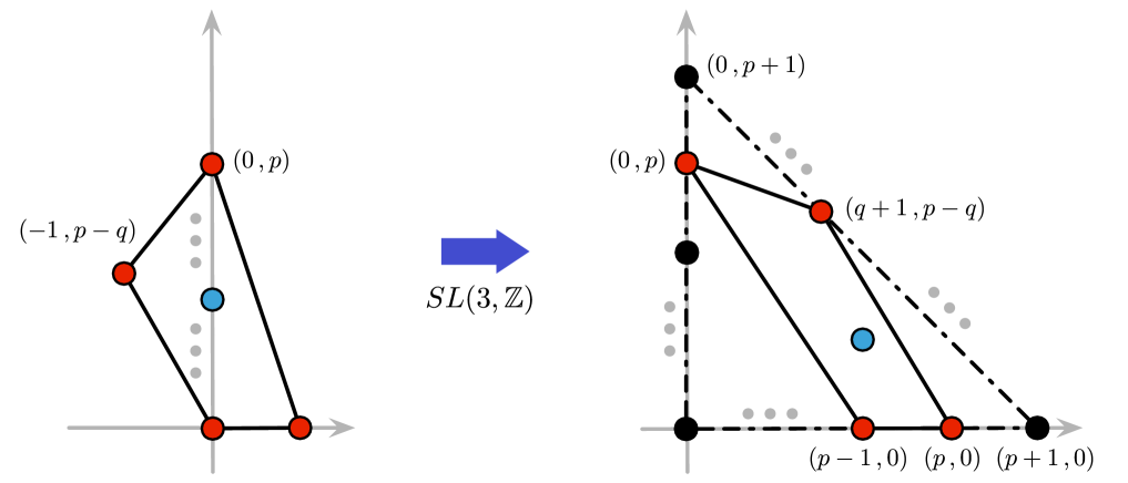
Figure 3: An embedding of $Y^{p,q}$ toric diagram in the toric diagram of $\mathbb{C}^{3}/\mathbb{Z}_{p+1}\times\mathbb{Z}_{p+1}$ orbifold theory. The linearly dotted gray points imply several internal vertices which are omitted for brevity.

The simplest example in this class would be local $\mathbb{F}_{0}$ surface, or $Y^{2,0}$, which engineers $D=5$ $SU(2)$ pure gauge theory. The detailed procedure of Higgsing toward $F_{0}$ is given as follows. Relabeling nodes of $\mathbb{C}^{3}/\mathbb{Z}_{3}\times\mathbb{Z}_{3}$ orbifold theory following (1.23), we have the superpotential

$$W=\frac{1}{3^{2}}\text{tr}\left(x_{14}y_{45}z_{51}-x_{14}z_{43}y_{31}+\cdots+x_{93}y_{31}z_{19}-x_{93}z_{38}y_{89}\right)\,.$$ (1.26)

A vev $v$ assigned to $z_{51}$ merges node $1$ and node $5$ of the orbifold theory as their relative $U(n)$ is frozen. By integrating out massive fields $x_{14}\,,x_{25}\,,y_{12}\,,y_{45}$, we have superpotential

$$\begin{split}\frac{1}{9}\text{tr}&\left(v^{-1}y_{16}z_{62}z_{27}x_{71}-v^{-1}x_{18}z_{84}z_{43}y_{31}+x_{36}y_{64}z_{43}-x_{36}z_{62}y_{23}\right.\\ &+x_{47}y_{78}z_{84}-x_{47}z_{76}y_{64}+x_{18}y_{89}z_{91}+x_{69}y_{97}z_{76}-x_{69}z_{91}y_{16}\\ &\left.-x_{71}z_{19}y_{97}+x_{82}y_{23}z_{38}-x_{82}z_{27}y_{78}+x_{93}y_{31}z_{19}-x_{93}z_{38}y_{89}\right)\end{split}$$ (1.27)

where the label $5$ is now renamed as $1$. By repeating similar exercise with four more FI constants turned on so that $x_{93}\,,y_{23}\,,y_{64}\,,x_{18}$ chiral fields are Higgsed one by one, we obtain the following superpotential

$$W_{\mathbb{F}_{0}}=\text{tr}\left(x_{23}y_{34}y_{41}z_{12}-x_{23}z_{34}y_{41}y_{12}+x_{41}y_{12}z_{23}z_{34}-x_{41}z_{12}z_{23}y_{34}\right)\,.$$ (1.28)

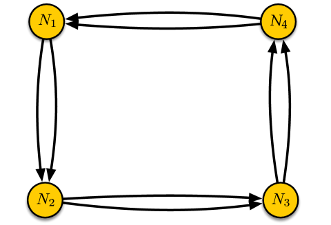
Figure 4: The quiver diagram of local $\mathbb{F}_{0}$ theory

Note we rescaled the chiral fields to avoid clutter then relabeled the nodes as follows,

$$5\,,8\rightarrow 1\,,\quad 6\rightarrow 2\,,\quad 3\,,9\rightarrow 3\,,\quad 7\rightarrow 4\,.$$ (1.29)

The quiver diagram of local $\mathbb{F}_{0}$ theory is drawn in Figure 4.

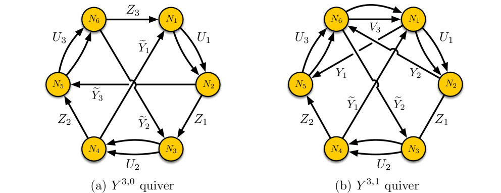
Figure 5: Quiver diagrams of $Y^{p,q}$ theory (a) with $p=3$, $q=0$ and (b) with $p=3$ , $q=1$. The chiral fields are labelled by the convention in [15].

A $D=5$ BPS quiver of higher rank gauge theory is obtained by starting with larger orbifold theories and by taking a similar Higgsing procedure, which truncates the corners of toric diagram according to Figure 3. For example, the BPS quivers of $SU(3)$ gauge theory are obtained by assigning vev to ten chiral fields in the orbifold probe quiver $\mathbb{C}^{3}/\mathbb{Z}_{4}\times\mathbb{Z}_{4}$. Figure 5 shows resulting $D=5$ BPS quivers for $SU(3)_{0}$ and $SU(3)_{1}$ gauge theory, respectively.

$X^{p,q}$ family and local $dP_{2}$ surface

Another class of toric Calabi-Yau 3-folds of interest is $X^{p,q}$ family, for two integers $p$ and $q$ such that $p>q\geq 1$. Its toric diagram has five external vertices

$$v_{1}=(1,0),\quad v_{2}=(0,0),\quad v_{3}=(0,p),\quad v_{4}=(-1,p-q),\quad v_{5}=(-1,p-q+1)\,.$$ (1.30)

An embedding of (1.30) to $\mathbb{Z}_{p+1}\times\mathbb{Z}_{p+1}$ orbifold’s toric diagram is sketched in Figure 6, which suggests how to obtain $D=5$ BPS quiver of $SU(p)_{q}$ gauge theory with a fundamental hypermultiplet, starting from the orbifold probe quiver via Higgsing.

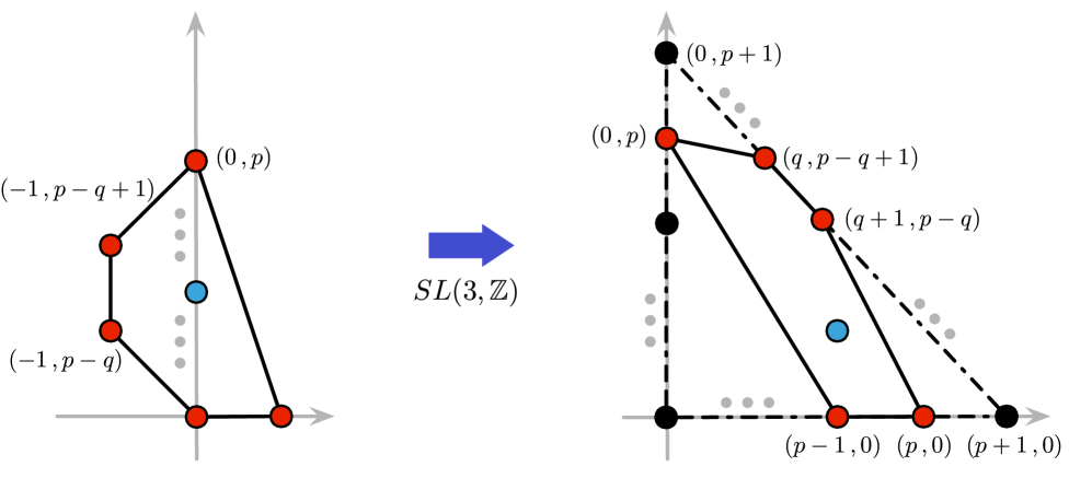
Figure 6: An embedding of $X^{p,q}$ toric diagram in the toric diagram of $\mathbb{C}^{3}/\mathbb{Z}_{p+1}\times\mathbb{Z}_{p+1}$ orbifold theory. The linearly dotted gray points imply several internal vertices which are omitted for brevity.

The simplest example in this family is $X^{2,1}$, also known as the local $dP_{2}$ geometry. Its BPS quiver can be explicitly worked out, as shown in Figure 7. This geometry turns out to engineer $D=5$ $SU(2)$ gauge theory with a fundamental hypermultiplet [26]. From the superpotential of $\mathbb{Z}_{3}\times\mathbb{Z}_{3}$ orbifold theory

$$W=\frac{1}{3^{2}}\text{tr}\left(x_{14}y_{45}z_{51}-x_{14}z_{43}y_{31}+\cdots+x_{93}y_{31}z_{19}-x_{93}z_{38}y_{89}\right)\,,$$

non-zero FI constants can lead vev assignment to $z_{51}\,,x_{93}\,,y_{23}\,,y_{64}$, which makes neighboring fields in the quiver massive. As we integrate out those massive, the superpotential becomes

$$\begin{split}W_{dP_{2}}=\text{tr}&\left(x_{34}y_{41}z_{12}z_{23}+x_{12}y_{23}y_{35}z_{51}-x_{45}z_{51}z_{12}y_{23}x_{34}\right.\\ &\left.+x_{45}x_{52}z_{24}-x_{12}z_{24}y_{41}-x_{52}z_{23}y_{35}\right)\,,\end{split}$$ (1.31)

where we relabeled the nodes in the quiver as follows,

$$6\rightarrow 1\,,\quad 3\,,9\rightarrow 2\,,\quad 7\rightarrow 3\,,\quad 5\rightarrow 4\,,\quad 8\rightarrow 5.$$ (1.32)

Note that if we further Higgs $x_{45}$ fields, we end up with local $\mathbb{F}_{0}$ theory superpotential in (1.28) and quiver in Figure 4 as the node $4$ and $5$ merge.

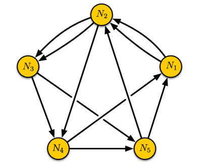
Figure 7: The quiver diagram of local $dP_{2}$ theory.

2 What to Count?

The problem we wish to address is the counting of BPS states which are particle-like with respect to the noncompact part of the spacetime, i.e., $\mathbb{R}^{3+1}$. Given the quivers of Section 1, it comes down to computing various topological invariants of such quiver dynamics such as refined Witten index, or cohomology if the dynamics reduces to a geometric one in the low energy limit. In practice, the former reduces to an exact path integral [10] or to a heat kernel computation of twisted partition function, while the latter can be sometimes computed explicitly if the geometry is simple enough, e.g., toric.

While either of such methods would work perfectly well when the dynamics is fully gapped, there is a general problem when the dynamics includes asymptotically flat directions. In particular, the problem arises invariably if the low energy theory involves an infinite volume of target manifold. All of the current examples involve local Calabi-Yau as part of the target, so such subtleties occur generically.

This is further compounded by the fine-tuned superpotential that is generically needed for local Calabi-Yau’s. The well-known machinery for exact path integrals, often broadly called “localization,” does not seemingly depend on details of the superpotential, but only with the hidden assumption of the genericity. Once we begin to impose non-Abelian global symmetries on the superpotential that cannot be entirely captured by flavor chemical potentials, the result of the localization computation often deviates significantly from the desired counting [27]. While the latter problem is also obliquely related to the noncompact nature of the target, it should be considered as a separate issue, and one can see by explicit exercises that the resulting JK residue computation [10] becomes rather ineffective even for the simplest examples.

Coming back to the specific counting problem at hand, note that the particle-like nature of BPS states means that the wavefunction of the states must be restricted to the $L^{2}$ class, i.e., square-normalizable with respect to the internal directions, while along $\mathbb{R}^{3+1}$ the state would propagate freely as plane wave. Even with more conventional and geometric approaches, such $L^{2}$ boundary condition is difficult to impose systematically for index problems. One well-known exception would be an asymptotically cylindrical non-linear sigma model (NLSM) where $L^{2}$ condition translates to the Atiyah-Patodi-Singer (APS) boundary condition [28].

As such, we will encounter two types of topological invariants. One class, which in this note would encompass many different types, computed by relatively straightforward existing routines, will be denoted as $\Omega$. It could be a result of the localization path integral or of the heat kernel computation; When the problem reduces to an entirely geometric one, such as via cohomology, we will also use $\Omega$ to denote index-like objects of singular homology or (compact) de Rham cohomology as well. The other, denoted as ${\cal I}$, would be the desired (refined) Witten index that counts physically relevant $L^{2}$ BPS states only.

The two objects are fundamentally different, despite that physics literatures tend to refer both as “index.” Only if the dynamics is compact and the Hilbert space is fully gapped, $\Omega={\cal I}$ is guaranteed. Much of what we explore in this note would be about how to recognize the difference, and, sometimes, how to extract ${\cal I}$ from $\Omega$ for these quiver theories.

In the path integral computation of the refined index, say, for those examples with fine-tuned superpotentials, one can seemingly evade such issues by turning on flavor chemical potentials associated with isometries. This essentially turns on mass terms and creates a gap. While the resulting partition function $\Omega$ has its own physical interpretation and is often very useful, e.g., for a check of dualities, such twisted partition functions sometimes give misleading results when it comes to the $L^{2}$ BPS state counting [27].

An almost trivial, yet illustrative example is a NLSM with target $\mathbb{C}^{1}$, say, realized in terms of a single massless chiral multiplet. The theory has a global symmetry that rotates $\mathbb{C}^{1}$ by a phase. Assigning a fugacity $x$ to this symmetry, likewise ${\bf y}$ for an $R$-symmetry, and vanishing R-charge to the single chiral multiplet to prohibit any superpotential, one finds the following twisted partition function from the localization of the path integral [10],

$$\Omega_{\mathbb{C}^{1}}=\frac{{\bf y}x^{-1/2}-{\bf y}^{-1}x^{1/2}}{x^{1/2}-x^{-1/2}}\,.$$ (2.1)

Turning off the flavor chemical potential, $x\rightarrow 1$, is impossible due to the pole, symptomatic of the noncompact dynamics.

Expanding in $x$ or $1/x$ might be the next tempting step, since $x$ enters the definition of $\Omega$ in the form of $x^{F}$ where $F$ is the flavor charge. This will at least give $F$-graded sectors, and the zeroth power of $x$ may have some chance of capturing the physics prior to the massive deformation due to $x$. However, the two expansions yield mutually inconsistent results at the invariant sector

$$\Omega_{\mathbb{C}^{1}}=\left\{\begin{array}[]{l}-{\bf y}^{-1}+O(1/x)\,,\\ -{\bf y}+O(x)\,.\\ \end{array}\right.$$ (2.4)

A general relation for fully gapped geometric theories says [29]

$${\cal I}=(-{\bf y})^{d}\chi_{y=-\bf y^{2}}\,,$$ (2.5)

where $d$ is the complex dimension of the compact target and $\chi_{y}$ is the Hirzebruch genus. The R-charge fugacity ${\bf y}$ grades the Hodge diamond diagonally, which should extend to any geometric theories, compact or not. The above expansion of $\Omega$ suggests that the content of the rotationally invariant BPS state corresponds to either one-dimensional $H^{2}$ or one-dimensional $H^{0}$, with all other cohomology empty. This follows from (2.4), combined with the fact that $\mathbb{C}^{1}$ is algebraic such that the Hodge diamond is populated by the vertical middle only.

Interestingly, these two conflicting results appear to reflect, respectively, de Rham cohomology $H^{\star}$ and de Rham cohomology with compact support $H^{\star}_{c}$,

$${\rm dim}\,H^{0}(\mathbb{C}^{1})={\rm dim}\,H^{2}_{c}(\mathbb{C}^{1})=1\ ;$$ (2.6)

(2.7)

$${\rm dim}\,H^{k}(\mathbb{C}^{1})={\rm dim}\,H^{2-k}_{c}(\mathbb{C}^{1})=0\ ,\quad k=1,2\,.$$ (2.8)

As we noted above, however, the physically relevant cohomology would be ${\cal H}^{\star}_{L^{2}}$, whereby one is supposed to count $L^{2}$ harmonic forms on the target, which is clearly absent for $\mathbb{C}^{1}$,

$${\cal H}^{\star}_{L^{2}}(\mathbb{C}^{1})=0\quad\rightarrow\quad{\cal I}=0\,.$$ (2.9)

This trivial example teaches us that neither the localization computation nor the standard (compact) de Rham cohomology computation should be trusted.

A more informative example can be found from an Abelian GLSM with $N$ chirals of charge $+1$ and $K$ chirals of charge $-1$. Suppose $N>K$ for simplicity and the sign of the FI constant such that this GLSM flows down to the $\mathcal{O}(-1)^{K}$ bundle over $\mathbb{P}^{N-1}$. Keeping a flavor symmetry that rotates all chirals simultaneously and forbidding superpotential by assigning zero $R$-charges to all chirals, we expand with respect to its fugacity $x$ and find

$$\Omega=\left\{\begin{array}[]{l}(-1)^{N-K-1}\left({\bf y}^{1-K-N}+\cdots+{\bf y}^{N-K-1}\right)+O(1/x)\,,\\ \\ (-1)^{N-K-1}\left({\bf y}^{1+K-N}+\cdots+{\bf y}^{N+K-1}\right)+O(x)\,.\\ \end{array}\right.$$ (2.13)

The flavor-neutral part, or the $x$-independent part, captures again precisely $H^{\star}$ and $H^{\star}_{c}$, respectively, of the bundle. The latter statement can be seen easily from the fact that $H^{\star}$ is homotopy invariant, so $H^{\star}$ of the bundle equals $H^{\star}(\mathbb{P}^{N-1})$, and also from the general fact that $H^{\star}_{c}$ is a Poincaré dual of $H^{\star}$.

What is ${\cal H}_{L^{2}}^{\star}$ of this bundle? As we will see in Sec. 3.1, there is a mathematical theorem which asserts that, under some favorable circumstances, ${\cal H}_{L^{2}}^{p}$ equals $H^{p}$ for $p>d$ where $d=N+K-1$ is the complex dimension. Also, the $L^{2}$ cohomology should come with natural pairing between ${\cal H}_{L^{2}}^{p}$ and ${\cal H}_{L^{2}}^{2d-p}$, forming Poincaré-dual pairs. This leaves behind only ${\cal H}^{d}_{L^{2}}$ undetermined. If $d$ happens to be odd, we can say more, since only even cohomologies are non-trivial,

$${\rm dim}{\cal H}_{L^{2}}^{2K}={\rm dim}{\cal H}_{L^{2}}^{2K+2}=\cdots={\rm dim}{\cal H}_{L^{2}}^{2N-2}=1\ ;$$ (2.14)

(2.15)

$${\rm dim}{\cal H}_{L^{2}}^{p}=0\ ,\quad\hbox{for all other }p\,.$$ (2.16)

These $L^{2}$ states can be compactly summarized via a truly enumerative index

$${\cal I}=(-1)^{N-K-1}\left({\bf y}^{1+K-N}+\cdots+{\bf y}^{N-K-1}\right)\,,$$ (2.17)

which is the rescaled Hirzebruch genus of the $L^{2}$ cohomology. One curious fact is that this result could have been obtained if we blindly took the common part of the two expansions of $\Omega$ in $x$ and $1/x$ as above [27], or equivalently the common part of $H^{\star}$ and $H^{\star}_{c}$. The latter is effectively the content of the theorem (3.3) below.

As these examples illustrate well, distinctive features of ${\cal I}$, as opposed to generic $\Omega$, are that it is integral, finite, and a symmetric Laurent polynomial in the $R$-charge fugacity ${\bf y}$. Note that, for BPS quivers in particular, the power of ${\bf y}$ is related to the spin and $SU(2)_{R}$-isospin content of the BPS spectra [29], so the invariance under ${\bf y}\rightarrow{\bf y}^{-1}$ is also a consequence of the spacetime symmetries on $\mathbb{R}^{3+1}$.

3 Abelian BPS Quivers

The main message above was how one must not be hasty and not resort to existing routines for supersymmetric partition functions or to (co-)homology of the internal manifold. When the latter is noncompact, the partition function will generically give misleading numbers while one must be also wary of exactly which cohomology is relevant for the problem at hand. As such, for some questions, the only reliable answer can be obtained from the direct cohomology counting, assuming that the distinction between $H^{\star}$, $H^{\star}_{c}$, and ${\cal H}_{L^{2}}^{\star}$ is carefully kept track of. For the toric case, on the other hand, there are systematic tools, available in Ref. [30] for example, that recover the homology $H_{\star}$ given the toric data, from which $H^{\star}$ can be inferred. We will presently turn to how one might further extract ${\cal H}_{L^{2}}^{\star}$ from such data.

We should warn the readers that even this is not going to be effective when the quiver turns non-Abelian; the low energy geometric limit of the latter often misses the relevant ground states of the quiver gauge theory as will be outlined in Section 4.

3.1 $L^{2}$ Cohomology from Homology

Let us start by reviewing a theorem in [31] which discussed relations between $L^{2}$ cohomology and following types of cohomology given a noncompact manifold ${\cal M}$ with scattering metric $g$ assigned;

• de Rham cohomology $H^{\star}({\cal M})$

• relative cohomology with respect to the boundary $H^{\star}({\cal M},\partial{\cal M})$

• de Rham cohomology with compact support $H^{\star}_{c}({\cal M})$

A metric $g$ on a manifold ${\cal M}$ is called the scattering metric when $g$ satisfies the following asymptotic behavior,

$$g\,\rightarrow\,\frac{dx^{2}}{x^{4}}+\frac{h}{x^{2}}\,,$$ (3.1)

where $x$ is a boundary defining function, i.e. $x$ vanishes but $dx\neq 0$ on $\partial{\cal M}$ and $h$ is a smooth metric on $\partial{\cal M}$. Note that if we set $x=1/r$, the scattering metric in (3.1) becomes

$$g\rightarrow dr^{2}+r^{2}h\qquad\text{with}\quad r\rightarrow\infty\,,$$ (3.2)

which reproduces a familiar form of metric on a conical geometry.

For a manifold ${\cal M}$ with scattering metric $g$, there exist natural isomorphisms,

$${\cal H}_{L^{2}}^{p}({\cal M})\rightarrow\begin{cases}H^{p}({\cal M}\,,\partial{\cal M})\,,&\text{if $p<m/2$}\,,\\ \text{Im}(H^{p}({\cal M}\,,\partial{\cal M})\rightarrow H^{p}({\cal M}))\,,&\text{if $p=m/2$}\,,\\ H^{p}({\cal M})\,,&\text{if $p>m/2$}\,,\end{cases}$$ (3.3)

with $m={\rm dim}_{\mathbb{R}}{\cal M}$, where ${\cal H}^{p}({\cal M}\,,\partial{\cal M})$ denotes the relative cohomology of ${\cal M}$ with respect to its boundary. For a complex manifold, such as Calabi-Yau $d$-folds, with $m=2d$, this means that ${\cal H}^{p}_{L^{2}}({\cal M})$ equals $H^{p}({\cal M})$ for $p>d$, determining the upper half of Betti numbers. This in turn determines the lower half as well since there is a natural pairing,

$$\int_{\cal M}\omega_{(k)}\wedge\omega_{(2d-k)}\ ,$$ (3.4)

which leaves only the middle cohomology ${\cal H}_{L^{2}}^{d}({\cal M})$ to be further considered. For our problem of local Calabi-Yau 3-fold, which are toric and thus algebraic, homology $H_{3}({\cal M})$ is empty, so both $H^{3}({\cal M})$ and ${\cal H}_{L^{2}}^{3}({\cal M})$ are also empty.

On the other hand, there is yet another natural pairing between $H^{p}$ and $H_{p}$ where the latter is the singular homology, as

$$\int_{\Sigma^{(p)}}\omega_{(p)}\ ,$$ (3.5)

so we arrive at

$${\rm dim}\,{\cal H}_{L^{2}}^{p}({\cal M}_{3})={\rm dim}\,{\cal H}_{L^{2}}^{6-p}({\cal M}_{3})={\rm dim}\,H_{6-p}({\cal M}_{3})\ ,\qquad p=0,1,2,$$ (3.6)

(3.7)

$${\rm dim}\,{\cal H}_{L^{2}}^{3}({\cal M}_{3})=0\ ,$$ (3.8)

for a toric Calabi-Yau 3-fold which is asymptotically conical. So, the matter of BPS state counting for Abelian quivers with unit rank at each node brings us to the homology counting for $p>3$.

Even before counting of $H_{p}({\cal M}_{3})$, we already know some universal facts. First, the toric Calabi-Yau 3-folds in question are all algebraic manifolds, with only even homology being non-trivial, meaning that only $H_{4}({\cal M}_{3})$ and $H_{6}({\cal M}_{3})$ are needed for extracting the entire ${\cal H}_{L^{2}}^{\star}({\cal M}_{3})$. Second, the local Calabi-Yau has the top homology empty, $H_{6}({\cal M}_{3})=0$ since one cannot possibly draw a top-dimensional simplex with no boundary. Therefore, one only needs to count $H_{4}({\cal M}_{3})$, whose dimension would also count ${\rm dim}{\cal H}_{L^{2}}^{2}({\cal M}_{3})={\rm dim}{\cal H}_{L^{2}}^{4}({\cal M}_{3})$.

Perhaps, the simplest examples of local Calabi-Yau 3-folds are the conifold and the local $\mathbb{P}^{2}$. These are, respectively, a $\mathcal{O}(-1)\oplus\mathcal{O}(-1)$ bundle over $\mathbb{P}^{1}$ and a $\mathcal{O}(-3)$ line bundle over $\mathbb{P}^{2}$. Given the homotopy invariance of singular homology, we are immediately led to

$$H_{\star}({\rm Conifold})=H_{\star}(\mathbb{P}^{1})\ ,\qquad H_{\star}({\rm local}\;\mathbb{P}^{2})=H_{\star}(\mathbb{P}^{2})\,,$$ (3.9)

which says ${\cal H}_{L^{2}}^{\star}({\rm Conifold})=0$ according to (3.3), for example, and one finds

$${\cal I}_{\rm Conifold}=0\ ,\qquad{\cal I}_{{\rm local}\;\mathbb{P}^{2}}=-{\bf y}-{\bf y}^{-1}\ .$$ (3.10)

The conifold example actually belongs to the class we already discussed in Section 2, except that $K\geq N$ where the $L^{2}$ cohomology vanishes entirely given the same sign of the FI parameter.

More relevant for us are the two well-known infinite classes of toric Calabi-Yau 3-folds introduced in Section 1.2. The first set is the $Y^{p,q}$ family, whose toric diagram is already given in Figure 3. For readers’ convenience, we list its four external vertices here again,

$$v_{1}=(1,0),\quad v_{2}=(0,0),\quad v_{3}=(0,p),\quad v_{4}=(-1,p-q)\,.$$ (3.11)

We take $q\neq p$, and also $q<p$ without loss of generality, such that in our convention the toric diagram is convex.

With this toric data, it is straightforward to compute their homology,

$$\begin{split}{\rm dim}\,H_{0}&=1\,,\\ {\rm dim}\,H_{2}&=p\,,\\ {\rm dim}\,H_{4}=&\,\,p-1\,,\\ {\rm dim}\,H_{6}&=0\,.\end{split}$$ (3.12)

In other words,

$${\rm dim}\,{\cal H}_{L^{2}}^{2}={\rm dim}\,{\cal H}_{L^{2}}^{4}=p-1\ ;\qquad{\rm dim}\,{\cal H}_{L^{2}}^{p}=0\ ,\;\;p\neq 2,4\,,$$ (3.13)

or

$${\cal I}_{Y^{p,q}}=(p-1)\times(-{\bf y}-{\bf y}^{-1})\ .$$ (3.14)

Recall that M-theory compactified on a $Y^{p,q}$ 3-fold results in $D=5$ $SU(p)_{q}$ gauge theory with the rank $p-1$.

Another infinite family of interest is the aforementioned $X^{p,q}$ family, whose toric diagram is shown in Figure 6. In addition to four vertices of $Y^{p,q}$ family, $X^{p,q}$ toric diagram has an extra vertex $v_{5}$ as noted in (1.30). We find the homology from the toric data as

$$\begin{split}{\rm dim}\,H_{0}&=1\,,\\ {\rm dim}\,H_{2}=&\,\,p+1\,,\\ {\rm dim}\,H_{4}=&\,\,p-1\,,\\ {\rm dim}\,H_{6}&=0\,,\end{split}$$ (3.15)

again with vanishing odd homology. Their $L^{2}$ cohomology ${\cal H}^{\star}_{L^{2}}$ is thus the same as that of $Y^{p,q}$ Calabi-Yau families, since only $H_{4}$ matters, such that

$${\cal I}_{X^{p,q}}=(p-1)\times(-{\bf y}-{\bf y}^{-1})\ .$$ (3.16)

M-theory compactified on an $X^{p,q}$ 3-fold, with $p>q$ and appropriately scaled, gives rise to a $D=5$ $SU(p)$ gauge theory with one fundamental matter, also of rank $p-1$.

3.2 What Have We Counted?

Let us take a step back and understand the physical states thus constructed from ${\cal H}_{L^{2}}^{2}({\cal M}_{3})\simeq{\cal H}_{L^{2}}^{4}({\cal M}_{3})$. The quivers with unit rank at each node correspond to states with a single KK charge only. What physical states in these gauge theories are counted by this counting? The answer is obvious; in the Coulomb phase the only BPS particles with neither the gauge charges nor the flavor charges are the rank-many vector multiplets that belong to the Cartan part of the gauge sector. Thus, the above song-and-dance ends up counting these Cartan vector multiplets, each with unit KK charge along the compactification circle $\mathbb{S}^{1}$.

More concretely, given a quiver with the Higgs moduli space ${\cal M}_{d}$, the Kähler 2-form $J$ defines the Lefschetz spin on differential $n$-forms, via $SU(2)_{L}$ actions,

$$L_{+}[\omega_{(n)}]=J\wedge\omega_{(n)}\ ,\qquad L_{-}[\omega_{(n)}]=J\lrcorner\,\omega_{(n)}\ \ ,\qquad L_{3}[\omega_{(n)}]=\frac{(n-d)}{2}\omega_{(n)}\ .$$ (3.17)

This $SU(2)_{L}$ has been identified as spatial angular momentum along $\mathbb{R}^{3}$, so we have counted the number of bound state pairs forming spatial spin doublets. This spin content comes about from the relative part of the dynamics, so it needs to be tensor-producted against the standard half-hypermultiplet content from $U(1)_{*}$. In other words, we would find vector multiplets out of ${\cal H}_{L^{2}}^{\star}({\cal M}_{3})$, whose number equals ${\rm dim}\,H_{4}({\cal M}_{3})$.

Indeed, the answers we found in Sec. 3.1 are all such that one finds spin 1/2 multiplets, the number of which always equals the purported rank of the corresponding $D=5$ supersymmetric field theory:

$${\cal I}_{(1,1,\dots,1)}({\bf y})={\rm rank}\times\left(-{\bf y}-{\bf y}^{-1}\right)\,.$$ (3.18)

So far, we have left out the center of mass motion along the spacetime $\mathbb{R}^{3+1}$, or equivalently the decoupled overall $U(1)$ vector multiplet, which supplies a half-hypermultiplet. The above spin doublets from the internal part combine with this half-hypermultiplet from $\mathbb{R}^{3+1}$ and elevate these states to rank-many vector multiplets. In the end, we have recovered the Cartan vector multiplets with a unit KK charge precisely via the proposed BPS quivers.

In some sense, through the above elaborate procedure, we did not really dig up any new information. After all, the rank of the gauge group should be equal to ${\rm dim}{\cal H}_{L^{2}}^{2}({\cal M}_{3})$, which, either by the Poincaré duality, or equivalently by the Lorentz symmetry, has to be the same as ${\rm dim}{\cal H}_{L^{2}}^{4}({\cal M}_{3})$. What must be noted is, rather, how this recovery for unit KK modes is achieved, only after a careful distinction between various types of cohomology, from the standard singular homology counting, via the theorem (3.3): We have counted ${\rm dim}{\cal H}_{L^{2}}^{2}({\cal M}_{3})$ by starting with the usual singular homology counting of toric variety whose $H_{4}$ maps to $H^{4}({\cal M}_{3})$ via the natural pairing and in turn to ${\cal H}_{L^{2}}^{4}({\cal M}_{3})$ by the theorem of Section 3.1, bringing us to

$${\rm dim}{\cal H}_{L^{2}}^{2}({\cal M}_{3})={\rm dim}{\cal H}_{L^{2}}^{4}({\cal M}_{3})={\rm dim}H_{4}({\cal M}_{3})\ ,$$ (3.19)

with all other ${\cal H}_{L^{2}}^{\star}({\cal M}_{3})$ empty, for local Calabi-Yau 3-folds.

4 Towers of Pure D0 Branes

Let us now turn to the question of how one constructs the entire KK towers for the Cartan vector multiplets; these pure KK states should correspond to assigning a common rank, say $n$, to all nodes of the BPS quiver. For each KK momentum $n$, one expects to find precisely rank-many spin doublets of supersymmetric ground states, to be tensored by a universal half-hypermultiplet from the decoupled $U(1)$. Recall that, despite various difficulties and subtleties, the problem for $n=1$ at least remains that of the cohomology of the Higgs moduli space. This is no longer true for $n>1$, as we see below.

4.1 Cohomology of the Symmetric Orbifold is Irrelevant

Since $n=1$ quiver was a single D0 probe theory over the Calabi-Yau ${\cal M}_{3}$, the Higgs branch for $n=1$ is precisely ${\cal M}_{3}$. This motivates one to speculate that $n>1$ quiver may flow down to a sigma model onto the $n$-th symmetric product of ${\cal M}_{3}$, say,

$$\mathcal{S}^{n}{\cal M}_{3}=({\cal M}_{3})^{n}/S_{n}\,.$$ (4.1)

Recall that the chiral multiplets in these BPS quivers are either adjoint or bifundamental: At typical point in the Higgs moduli space, the bifundamentals are turned on and reduce the gauge groups to a single $U(n)$, namely, the common $U(n)_{*}$ that rotates all nodes simultaneously. Among this $U(n)_{*}$, the overall $U(1)_{*}$ decouples from the rest of the dynamics since no bifundamentals would be rotated by it, and its scalar superpartners serve as the center of mass degrees of freedom along the spatial $\mathbb{R}^{3}$. This leaves behind the interacting $SU(n)_{*}$ theory, under which all chirals transform as adjoint. This leads us to the above symmetric orbifold.

One may hope that the (co-)homology of this symmetric orbifold is the quantity to study. However, this is not correct. There are two interrelated problems with this naive thought. The first is that the theory actually flows to a different symmetric orbifold,

$${\cal N}_{n}\equiv\left[({\cal M}_{3})^{n}\times(\mathbb{R}^{3})^{n}\right]/S_{n}=\mathbb{R}^{3}\times\left[({\cal M}_{3})^{n}\times(\mathbb{R}^{3})^{n-1}\right]/S_{n}\,,$$ (4.2)

where $(\mathbb{R}^{3})^{n}$ comes from the Coulombic side. This is because, at generic Higgs vev of bifundamental chirals and adjoint chirals of the probe theory, the Cartan part of $SU(n)_{*}$ remains massless as well, so these Coulombic moduli can be turned on simultaneously along with the chirals. Since we are dealing with quiver GLSM with four supercharges, the former translates to $3(n-1)$ free Coulombic moduli, i.e. relative positions of $n$ D0 branes in the spatial $\mathbb{R}^{3}$. Now, the orbifolding group $S_{n}$ is the Weyl group of $SU(n)_{*}$, so it would act on the Coulombic moduli and Higgs moduli simultaneously, giving us the second factor in the rightmost expression of (4.2).

The second problem concerns, again, the obligatory $L^{2}$ condition along all moduli direction, except for a single $\mathbb{R}^{3}$ factor which is the center of mass. In other words, the wavefunction must be $L^{2}$ on ${\cal N}_{n}/\mathbb{R}^{3}$. There is a well-established generating function that keeps track of Poincaré polynomial of a symmetric orbifold, $\mathcal{S}^{n}{\cal M}$, given that of ${\cal M}$, due to Macdonald [32]. However, as illustrated in the Appendix A, one can understand the counting from this generating function merely as that of $n$ identical particle quantum mechanics with Bose statistics imposed.

This means that any such $n$-particle states would be plane-wave-like along each and every factor of $\mathbb{R}^{3}$’s in ${\cal N}_{n}$. Even though one started with non-trivial $L^{2}$ wavefunctions found in ${\cal M}_{3}$, there is no mechanism at the level of the orbifold dynamics that forces two or more of them to be confined along the Coulombic part of the relative motion, $(\mathbb{R}^{3})^{n-1}$, for $n>1$. As such, even if there are normalizable BPS states at $n=1$, no other normalizable states can be found for $n>1$ at the level of $L^{2}$ cohomology of ${\cal N}_{n}/\mathbb{R}^{3}$, regardless of details of ${\cal M}_{3}$.

4.2 Entire KK Towers of the Cartan

If the $L^{2}$ cohomology of the low energy orbifold fails to capture the desired BPS spectrum, we must step back to the quiver GLSM. One might think that topological invariants must be the same between these two theories since one is merely the low energy limit of the other, but in reality we just saw that this is too naive, which is of course ultimately related to how the naive robustness often fails in the presence of the continuum sectors [11, 27]. As we saw above, the problem stems not only from the noncompact Calabi-Yau but also from the Coulombic continuum.

A relatively simple example where GLSM and its low energy limit thereof would offer different indices and twisted partition functions is that multi D0 dynamics, namely maximally supersymmetric $SU(n)$ Yang-Mills quantum mechanics. The low energy limit is the symmetric orbifold $\mathbb{R}^{9(n-1)}/S_{n}$ as the target, and the twisted partition function has been computed in the past [27], with the unrefined limit being [33, 34, 36, 35]

$$\Omega_{\mathbb{R}^{9(n-1)}/S_{n}} = \frac{1}{n^{2}}\,,$$ (4.3)

$$\Omega_{SU(n)} = \sum_{p|n}\frac{1}{p^{2}}=1+\cdots+\frac{1}{n^{2}}\ ,$$ (4.5)

where, in the latter, $p$’s are divisor of $n$ including $1$. Note how the two offer different twisted partition functions. This goes against the naive thought that such quantities are topological and thus should agree between UV and IR pictures.

We will see presently how the integral indices ${\cal I}$, not just twisted partition functions $\Omega$, differ between the two descriptions. The twisted partition functions are rational, again due to the asymptotically flat and gapless directions. The integral index that counts the $L^{2}$ bound state requires a subtraction of the latter continuum contribution, usually denoted as $\delta{\cal I}$, such that

$${\cal I}_{\mathbb{R}^{9(n-1)}/S_{n}} = \Omega_{\mathbb{R}^{9(n-1)}/S_{n}}+\delta{\cal I}_{\mathbb{R}^{9(n-1)}/S_{n}}\,,$$ (4.6)

$${\cal I}_{SU(n)} = \Omega_{SU(n)}+\delta{\cal I}_{SU(n)}\,.$$ (4.8)

As one can show using the heat kernel method, the defect terms $\delta{\cal I}$’s are determined entirely by the asymptotic dynamics of the either system [33, 34].

On the other hand, as one approaches the asymptotic region, the orbifold becomes an ever more accurate approximation of the GLSM, since all masses of off-diagonal parts, dropped in favor of the orbifold, scale linearly with the Coulombic vev. This implies, given the general nature of $\delta{\cal I}$ as a boundary contribution [33],

$$\delta{\cal I}_{SU(n)} = \delta{\cal I}_{\mathbb{R}^{9(n-1)}/S_{n}}+\cdots\ ,$$ (4.9)

where the ellipsis denotes terms that arise from hybrid sectors with multiple partial bound states exploring the asymptotic regions individually. This cascade of partial bound states contributing to $\delta{\cal I}$ was observed early on [36, 37].

The $SU(n)$ theory is a little special in that the only contributing continuum sectors are such that $n$ is divided equally to $p$ identical $n/p$-particle bound states formed by $SU(n/p)$ interactions, whose mutual asymptotic dynamics is governed by $\mathbb{R}^{9(p-1)}/S_{p}$. This implies

$$\delta{\cal I}_{SU(n)} = \sum_{p|n}^{p\neq 1}\delta{\cal I}_{\mathbb{R}^{9(p-1)}/S_{p}}\times{\cal I}_{SU(n/p)}\ ,$$ (4.10)

with which the only self-consistent answer in the end is

$$\delta{\cal I}_{\mathbb{R}^{9(n-1)}/S_{n}} = -\Omega_{\mathbb{R}^{9(n-1)}/S_{n}}\,,$$ (4.11)

$${\cal I}_{\mathbb{R}^{9(n-1)}/S_{n}} = 0\,,$$ (4.13)

$${\cal I}_{SU(n)} = 1\,.$$ (4.15)

The last supports the existence of the M-theory as was originally envisioned by Witten [38].

One can understand this disparity between the GLSM and the low energy orbifold limit more physically as follows: As Polchinski demonstrated handsomely [39], a simple virial theorem, combined with supersymmetry, shows that, on the supersymmetric ground state in question, the expectation values of squared matrix elements are of similar size between the “diagonal” and “off-diagonal” part of $SU(n)$. Therefore, if one scales down the energy scale toward infrared to render the off-diagonal components to become very massive and “ignorable,” the support of the wavefunction is shrunken further and further near the origin along the Cartan directions as well. In the strict geometric limit, such wavefunctions would then have a vanishing support and becomes undetectable by $d=1$ orbifold.

Interestingly, this prototype $SU(n)$ example is in fact all one needs to address the infinite KK towers of the Cartan part of the gauge sector that we are trying to establish. Why is so? Although the orbifold ${\cal N}_{n}$ is on its own irrelevant for BPS state counting as we already saw, this moduli space is still useful for visualizing where the desired bound states are supported. Consider $(n,n,n,\cdots,n)$ quiver with the moduli space

$${\cal N}_{n}=\mathbb{R}^{3}\times\left[({\cal M}_{3})^{n}\times(\mathbb{R}^{3})^{n-1}\right]/S_{n}\,.$$ (4.16)

We have seen in the previous section that $n=1$ case produces rank-many spin doublets along ${\cal M}_{3}$, each of which is combined with a half-hyper from the center of mass $\mathbb{R}^{3}$ to form a vector multiplet. Let us denote the wavefunction responsible for these states,

$$\Psi_{\rm geometric}\$$ (4.17)

collectively. These states can be characterized as plane-wave-like with half-hyper spin content along $\mathbb{R}^{3}$ and as an $L^{2}$ harmonic 2-form/4-form pair along ${\cal M}_{3}$.

Recall that, at generic point of the Coulomb phase of geometrically engineered $D=5$ gauge theory, ${\cal M}_{3}$ is a smooth manifold and point-wise can be approximated by $\mathbb{C}^{3}=\mathbb{R}^{6}$. If we scale the quiver theory such that the symmetric orbifold is better and better approximation, the desired states must be that unit-charged KK particles are clustered ever closer among themselves, such that the above symmetric orbifold is better and better approximated by

$${\cal N}_{n}\simeq[\mathbb{R}^{3}\times{\cal M}_{3}]\times\left[(\mathbb{R}^{6})^{n-1}\times(\mathbb{R}^{3})^{n-1}\right]/S_{n}\,.$$ (4.18)

The former square bracket represents the center of mass part of the dynamics while the latter is approximately valid when the distances between the individual bound states of the $(1,1,1,\cdots,1)$ sub-quivers are relatively small compared to the curvature scale of ${\cal M}_{3}$.

The relative part,

$$\left[(\mathbb{R}^{6})^{n-1}\times(\mathbb{R}^{3})^{n-1}\right]/S_{n}=(\mathbb{R}^{9})^{n-1}/S_{n}$$ (4.19)

can be regarded as the low energy limit of the $SU(n)_{*}$ subsector we have introduced in Section 1 for the orbifold examples. However, we must emphasize again that one cannot expect to find the relevant $L^{2}$ states at this geometric level. Rather, the states in question, if any, would emerge only if we go back to the full GLSM. Therefore, the desired wavefunctions may be approximately factorized as

$$\Psi\simeq\Psi_{\rm geometric}\otimes\Psi_{SU(n)_{*}}$$ (4.20)

at least in the limit where the moduli space itself factorizes approximately as in (4.18).

Let us see more precisely how this happens. The two factors, $\Psi_{\rm geometric}$ and the relative part of the wavefunction, which is to be eventually replaced by $\Psi_{SU(n)_{*}}$, scale somewhat differently under change of parameters of the quiver theories. $\Psi_{\rm geometric}$ is represented by a $L^{2}$ harmonic form on ${\cal M}_{3}$, so its support is sensitive to the scale of the Calabi-Yau 3-fold in question, or equivalently to FI constants of the BPS quiver. On the other hand, the relative part of the wavefunctions is unaware of the FI constants and scales with the gauge couplings. As one tunes the coupling so that the symmetric orbifold limit is ever more accurate, the support of the relative part of the wavefunction must become more and more localized at the origin of the orbifold. On the other hand, near this origin, the moduli space is increasingly similar to (4.18), and the relative part of the quiver dynamics approaches the $SU(n)_{*}$ theory.

One parameter that controls this process is the gauge coupling, since the massive off-diagonal component, to be dropped in the orbifold limit, would have the mass proportional to the coupling. This means that, by tuning the electric couplings of the BPS quiver continuously (but never actually taking the limit), one can make the support of the relative part much smaller than the support of $\Psi_{\rm geometric}$. Therefore there exists a corner of the parameter space of the BPS quiver, where we can reliably replace the BPS state counting problem by that of (4.20). This approximation is possible unless we are sitting near a singular point of the center of mass ${\cal M}_{3}$. We are considering generic point on the Coulombic moduli space of $D=5$ theory, so ${\cal M}_{3}$ would be smooth everywhere. As such, (4.20) is reliable at least for the purpose of the index counting for BPS states,

We have uncovered, earlier in this section, the content of $\Psi_{\rm geometric}$ as rank-many vector multiplets, it remains to count $\Psi_{SU(n)_{*}}$ by going back to the approximate $SU(n)_{*}$ theory. Fortunately, this more difficult task is already performed since $SU(n)_{*}$ theory is nothing but the maximally supersymmetric Yang-Mills theory which we used above as an illustration. Our review above immediately translates to

$${\cal I}_{SU(n)_{*}} = 1\ ,$$ (4.21)

implying a unique supersymmetric $\Psi_{SU(n)_{*}}$ for each integer $n$. This should be contrasted against

$${\cal I}_{(\mathbb{R}^{9})^{n-1}/S_{n}} = 0\ ,$$ (4.22)

which supports our earlier claim that cohomology of the symmetric orbifold does not have new localized states “created” due to the orbifolding. The gauge theory “resolution” of the orbifold singularity is essential for $d=1$.

As such, the BPS state content of any orbifold quiver is such that there are again precisely rank-many vector multiplets at each and every KK charge $n$; There is always a unique $\Psi_{SU(n)_{*}}$ state, so the counting of the states are the same for all $n\geq 1$. This translates to the following refined $L^{2}$ index for $(n,n,\dots,n)$ quivers,

$${\cal I}_{(n,n,\dots,n)}({\bf y})={\rm rank}\times\left(-{\bf y}-{\bf y}^{-1}\right)$$ (4.23)

universally where “rank” refers to $D=4,5$ field theory in question. The result is manifestly independent of the potential wall-crossing chambers, since the relevant bound state comes from an effective $SU(n)_{*}$ theory that has no FI parameter.

We have obtained this $SU(n)_{*}$ theory rather explicitly for orbifold quiver theories; recall $U(n)_{*}$ and $SU(n)_{*}$ theories we discussed in Section 1. The two are related by how we factor out the decoupled overall $U(1)$ and keep only the traceless parts of chirals $x,y,z$, which we called $x_{*},y_{*},z_{*}$. The cubic superpotential,

$$W_{*}={\rm tr}(x_{*}[y_{*},z_{*}])$$ (4.24)

governs the low energy dynamics, rendering this $SU(n)_{*}$ theory to become the maximally supersymmetric $SU(n)$ theory, leading us to (4.21), and the resulting rank-many vector multiplets for each $n>1$.

Furthermore, the spirit behind the decompositions (4.18) and (4.20) clearly holds for any smooth Calabi-Yau 3-fold ${\cal M}_{3}$, as long as the curvature length scale of the latter is taken sufficiently large and the support of the relative part of the wavefunction is controlled to be small by tuning the electric coupling. As such, this result of KK towers of rank-many vector multiplets still stands universally, although our line of thoughts cannot be applied immediately to central, strongly interacting regions of the Coulombic moduli space of $D=5$ theory in question.

Although we did this for positive $n$, the same for negative $n$ also follows since nothing much changes upon $n\rightarrow-n$ except which half supersymmetries of the $D=5$ theory are preserved by the BPS state.

5 Coulombic Counting

In recent years, computations of (refined) index for supersymmetric gauged quantum mechanics have received renewed interest via the localization method. While the most sweeping formulation of such kind was given several years ago [10], via Jeffrey-Kirwan residues, this does not quite work for the BPS quivers here since the former must assume that the superpotential is generic.

Although some global symmetries can be incorporated, allowing the superpotential constrained further, non-Abelian global symmetries are often not entirely reflected; Asymptotic isometries of local Calabi-Yau’s in question, cannot be fully incorporated into such a computation. One might still hope that the Cartan part of such isometries, whose chemical potentials do enter the computation, suffices but one can see in various local Calabi-Yau examples, such as the conifold quiver, the routine offered by these localization computation often produces nonsensical results.

One alternative is an older routine of the Coulomb branch counting [40, 41, 42, 43], whose mechanism by itself is insensitive to the superpotential of the quiver since it keeps track of how BPS states are constructed along the Coulombic moduli space; the superpotential data enters obliquely, if crucially, via the single-center degeneracies treated as input data, also known as the quiver invariant.

In this approach, the issues due to noncompact targets are split into two different types. The subtleties due to the noncompact Higgs branch are now all hidden in the quiver invariant [44, 29] to be surmised through other routes. For our quivers, in particular, the ubiquitous spectra of the neutral KK tower we have already obtained restrict many of quiver invariants to vanish. The other type due to the Coulombic continuum has a known resolution in existing wall-crossing literature via a form of multi-cover formulae [45, 40, 41, 27]. Rational invariants from the latter, again to be denoted as $\Omega$ here, have an explicit inversion formula and give ${\cal I}$ as needed. We will see how these work, first by revisiting multi-D0 states.

5.1 Pure D0 Towers Revisited, with Quiver Invariants

For general quiver theories, this multi-center approach is known to be incomplete due to the so-called quiver invariants, which count degeneracies of single-center BPS objects and are immune to wall-crossing [47, 29, 44, 48]. States counted by the quiver invariants are localized at the center of the Coulombic moduli space and instead spread along the Higgs branch. This means that the missing superpotential data which affects the Higgs branch only, would manifest in this Coulombic approach via the quiver invariants, often denoted as $\Omega_{S}$ or $\Omega_{\rm Inv}$ and generally rational if the quiver is not primitive. We use ${\cal I}_{S}$ for their integral and enumerative counterpart for the sake of clarity.

One can view ${\cal I}_{S}$ as an analog of the internal degeneracy, 2, of an electron which is needed to construct Schrödinger atoms. A general solution [40, 41, 42] to the wall-crossing formulae of Kontsevich and Soibelman [45] exists [46], with the quiver invariants as input data. On the other hand, ${\cal I}_{S}\neq 0$ appears generically in the black hole regime, and the known BPS spectra of $D=4$ field theories tend to be consistent with ${\cal I}_{S}=0$ except for the $U(1)$ single-node quivers. Even with generic superpotentials, as would be relevant for BPS black holes, the quiver invariant tends to be absent when all intersection numbers are 2 or smaller [47, 44, 29].

States counted by the quiver invariant are in particular dictated by the F-term embedding into D-term ambient [29]. As such, the simpler, fine-tuned superpotential tends to suppress these possibilities further. A simple and non-trivial example is the triangle cyclic quiver [48] with the common intersection number 3. For this, the Coulomb counting gives ${\cal I}=-{\bf y}-{\bf y}^{-1}+{\cal I}_{S}$ with ${\cal I}_{S}$ unknown. With generic superpotentials, the quiver theory flows to an elliptic curve such that ${\cal I}=0$ and thus ${\cal I}_{S}={\bf y}+{\bf y}^{-1}$ [44]. The same quiver with a fine-tuned superpotential with $SU(3)$ isometry, on the other hand, would flow to a local $\mathbb{P}^{2}$, for which we must have ${\cal I}=-{\bf y}-{\bf y}^{-1}$ and ${\cal I}_{S}=0$.

With the simplifying assumptions that ${\cal I}_{S}=0$ except for the elementary nodes, we have computed the Coulombic index of several $D=5$ BPS quivers with $(n,n,\dots,n)$ rank vectors, and successfully reproduced,

$${\cal I}(n\hbox{ D0's};{\bf y})={\rm rank}\times\left(-{\bf y}-{\bf y}^{-1}\right)\ ,$$ (5.1)

independent of $n$. Again, “rank” refers to $D=4,5$ field theory in question. Note that the mutual consistency between our counting in Section 3 and 4 and the current Coulombic counting requires

$${\cal I}_{S}(n\hbox{ D0's};{\bf y})=0\ ,$$ (5.2)

in particular, and ${\cal I}_{S}=0$ for all nontrivial subquivers as well.

The index ${\cal I}(n\,\hbox{D0's};{\bf y})$ is independent of the wall-crossing chambers. This chamber-independence has been seen from the construction of Section 3 and 4; only $\Psi_{\rm geometric}$ part can know about FI constants, $\zeta$, but the degeneracy is insensitive to signs of $\zeta$ since the topology remains independent thereof. The stability is also numerically observed here, but more generally, the Coulombic wall-crossing picture implies the same for all states whose quiver rank vectors are in the kernel of the intersection matrix [49].

When $n>1$ so that the quiver is no longer primitive, an important distinction must be made between the true integral index ${\cal I}$ and its rational cousin $\Omega$. $\Omega$ could be directly computed by a Coulombic heat kernel method [40, 9], from which ${\cal I}$’s are extracted by inverting

$$\Omega(\Gamma;{\bf y})=\sum_{p|\Gamma}\frac{{\bf y}-{\bf y}^{-1}}{p\cdot({\bf y}^{p}-{\bf y}^{-p})}\cdot{\cal I}(\Gamma/p;{\bf y}^{p})\ ,$$ (5.3)

where the sum is over divisors $p$ of the rank vector $\vec{N}$ of quiver $\Gamma$ and $\Gamma/p$ refers to a subquiver, whose rank is given by division of $\vec{N}$ by $p$. This sum is exactly the kind of the rational structure, now refined, that we have encountered for $\Omega_{SU(n)}={\cal I}_{SU(n)}-\delta{\cal I}_{SU(n)}$ via (4.10) for maximally supersymmetric $SU(n)$ theories. The quiver invariant follows the same pattern, so $\Omega_{S}(n\hbox{ D0's};{\bf y})=0$.

5.2 Electrically Charged BPS States in the Weak Coupling Chamber

For BPS states with charges coming from the gauge sector, one should expect heavy wall-crossings to happen. Already with such a relatively simple theory like $D=4$ $SU(2)$ $N_{f}=4$, the wall-crossing pattern quickly becomes intractable, so the situation with $D=5$ BPS quivers, with two extra nodes relative to its $D=4$ counterpart, any sort of classification of BPS states is not going to be practical. Any such attempt of BPS state classification should be in practice accompanied by well-motivated choices of the wall-crossing chamber.

One type of the chamber which might be viewed as a reference is the weak coupling chamber. Note that the weak coupling limit by itself does not preclude wall-crossings since dyons can decay to a pair of other dyons easily when the rank of the group is larger than one [50, 51, 52]. For purely electric objects from the gauge group choice and the matter content, however, there should not be any wall-crossing in the weak coupling limit since the theory would be defined by such content. As such, the ”weak coupling chamber” makes sense for these elementary BPS objects with a relatively simple state counting: Given how a KK tower would result from the $\mathbb{S}^{1}$ compactification, we should expect to find

$${\cal I}(\Gamma+n\hbox{ D0's})={\cal I}(\Gamma)$$ (5.4)

for quiver $\Gamma$ whose net charge content corresponds to an elementary state that defines the $D=5$ field theory in question.

Let us recall what we know about the weak coupling regime of $D=4$ pure $SU(2)$ theory. The weak coupling means very large $1/g^{2}$, so the monopole $M$ and the dyon $D$, which together span all known BPS states of $D=4$ pure $SU(2)$, would be much heavier than the elementary charged vector boson $W$,

$$|Z_{M}|\gg|Z_{W}|\ ,\qquad|Z_{D}|\gg|Z_{W}|\ ,$$ (5.5)

while the central charges are related as $Z_{W}=Z_{M}+Z_{D}$. Drawing these three central charges in the upper half plane, $Z_{M}$ and $Z_{D}$ have to be very large and point to almost opposite of each other, while $Z_{W}$ should direct the halfway between the two. On the other hand, FI constants measure how far the central charges of each node, $Z_{M}$ and $Z_{D}$, deviate from the total central charge, $Z_{M}+Z_{D}$ [8, 9]. Therefore, the weak coupling chamber corresponds to a large FI constant of some particular sign, opposite of the other strong coupling chamber where $W$ is absent as a state.

How does this generalize to $D=5$ pure $SU(2)$ theory? The question comes down to understanding the central charges of the two additional nodes. For $\mathbb{F}_{0}$ quiver in Figure 9 of Appendix B, the magnetic charge assignment to each node is

$$M\ ,\quad-M\ ,\quad-M\ ,\quad M\ ,$$ (5.6)

so one might think that signs of the FI constants should follow these signs. On a closer inspection, however, one realizes that there are more charge components to the latter two whose central charge contributions scale like $1/g^{2}$,

$$M\ ,\quad-M\ ,\quad I-M\ ,\quad M-I\ ,$$ (5.7)

with $I$ denoting the instanton. In fact, $I-M$ corresponds to the so-called KK monopole, which is present whenever a $D\geq 4$ gauge theory is put on a circle, in such a way that the full instanton $I$ is recovered from $M+(I-M)$ [53].

The last node with magnetic charge $M-I$ carries the KK charge but the latter’s central charge contribution $\sim 1/R$ scales differently, as it does not get renormalized with the gauge coupling renormalization. Pure electric central charge, which should be added to the various nodes, would also scale with $1/R$, in the regime where the bulk of their mass comes primarily from the $\mathbb{S}^{1}$ holonomy vev. In such a weak coupling regime, neither of these additional types of charges is the leading contribution to the central charges of the elementary nodes.

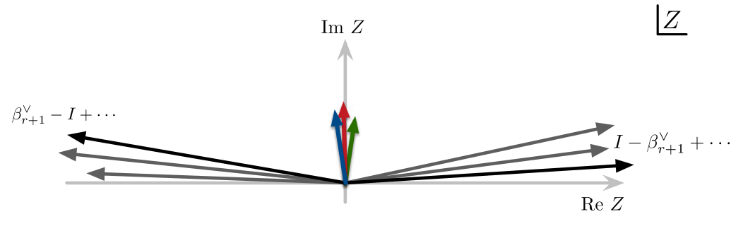
Figure 8: In the weak coupling limit, the elementary nodes are categorised into three classes according to their central charges. The first, short arrows in the middle, are weak coupling objects, such as quarks and charged vectors. The second are rank-many objects with positive magnetic charges, $\beta_{i\leq r}^{\vee}$, plus the KK monopole, $I-\beta^{\vee}_{r+1}$. These are long arrows to the right. The third group with the opposite magnetic/instanton charges points toward the left. If the total central charge consists only of electric, flavor, and KK charges, the second and the third classes of nodes would be equipped with large positive and large negative FI constants, respectively.

Therefore, in the weak coupling limit achieved by a small $\mathbb{S}^{1}$ radius $R$ and large Wilson line expectation values $\sim 1/R$, the node 1 and the node 3 each should then have large positive FI constant while node 2 and node 4 should have large negative FI constant. Since the FI constants measure deviation of the node central charges away from the total central charge of the quiver, this characterization is robust whenever the total charge of the quiver has neither magnetic nor instanton components.

This story generalizes to all higher rank gauge theories with or without flavors. For example, consider a $D=5$ theory with a rank $r$ simple gauge group and $N_{f}$ fundamental hypermultiplets; the number of nodes for the BPS quiver is $2r+2+N_{f}$. Of these, $N_{f}$ captures the matter electric charges and bare flavor masses thereof, while $2r+2$ nodes are analog of the monopole node and the dyon node of pure $D=4$ $SU(2)$ BPS quiver.

With simple roots $\{\beta_{i}\}$, $2r$ nodes of $D=4$ BPS quiver would have magnetic charges with the dual root $\beta_{i}^{\vee}$ [54]

$$\beta^{\vee}_{1}\ ,\quad-\beta^{\vee}_{1}\ ,\quad\beta^{\vee}_{2}\ ,\quad-\beta^{\vee}_{2}\ ,\quad\dots\quad,\quad\beta^{\vee}_{r}\ ,\quad-\beta^{\vee}_{r}\ .$$ (5.8)

The rest of the nodes, if flavor hypermultiplets are present, corresponds to these elementary matter BPS states [55].

On top of these, $D=5$ BPS quiver requires two additional nodes which, respectively, should carry the magnetic and the instanton charges as [53, 56]

$$I-\beta^{\vee}_{r+1}\ ,\qquad\beta^{\vee}_{r+1}-I\ ,$$ (5.9)

where $\beta^{\vee}_{r+1}\equiv\sum a_{i}^{\vee}\beta^{\vee}_{i}$ is the highest dual root. Recall that $h^{\vee}=\sum a_{i}^{\vee}$ is the dual Coxeter number and $\{\beta_{1}^{\vee},\cdots,\beta_{r}^{\vee},-\beta_{r+1}^{\vee}\}$ span the affine Dynkin diagram of the dual group.

Again, the weak coupling chamber translates to large positive FI constants for nodes with magnetic charges, $\beta_{i\leq r}^{\vee}$ and $-\beta^{\vee}_{r+1}$, and large negative FI’s for nodes with magnetic charges, $-\beta_{i\leq r}^{\vee}$ and $\beta^{\vee}_{r+1}$. With such an assignment, one should be able to recover, from the $D=5$ BPS quiver, the expected KK towers of elementary fields, such as charged vector mesons, collectively denoted as W, and quarks, also collectively Q, if fundamental flavors are added; that is

$${\cal I}(\hbox{W}+n\hbox{ D0's})={\cal I}(\hbox{W})=-{\bf y}-{\bf y}^{-1}\ ,$$ (5.10)

(5.11)

$${\cal I}(\hbox{Q}+n\hbox{ D0's})={\cal I}(\hbox{Q})=1\ .$$ (5.12)

We have tested this for various BPS quivers we have discussed. See Table 1, where we scanned up to 11 particle problems and also confirmed that the index is robust under small variation of FI constants.

$\vec{N}$ BPS states ${\cal I}$ FI constants $\mathbb{F}_{0}$,   pure $SU(2)$,   $\zeta_{\text{w}}=C(1,-1,1,-1)$ $(1,1,0,0)$ W $-{\bf y}-{\bf y}^{-1}$ $\zeta_{\text{w}}$ $(2,2,1,1)$ W + KK $-{\bf y}-{\bf y}^{-1}$ $\zeta_{\text{w}}\pm\epsilon(1,-1,-1,1)$ $(3,3,2,2)$ W + 2 KK $-{\bf y}-{\bf y}^{-1}$ $\zeta_{\text{w}}\pm\epsilon(1,-1,-1,1)$ $\mathbb{F}_{1}$,   pure $SU(2)_{\pi}$,   $\zeta_{\text{w}}=C(1,-1,1,-1)$ $(1,1,0,0)$ W $-{\bf y}-{\bf y}^{-1}$ $\zeta_{\text{w}}$ $(2,2,1,1)$ W + KK $-{\bf y}-{\bf y}^{-1}$ $\zeta_{\text{w}}\pm\epsilon(1,-1,-1,1)$ $dP_{2}$,   $SU(2)$ with $N_{f}=1$,   $\zeta_{\text{w}}=C(1,-1,1,0,-1)$ $(1,1,0,0,0)$ W $-{\bf y}-{\bf y}^{-1}$ $\zeta_{\text{w}}$ $(2,2,1,1,1)$ W + KK $-{\bf y}-{\bf y}^{-1}$ $\zeta_{\text{w}}\pm\epsilon(1,-1,-1,1,0)$ $(1,1,1,2,1)$ Q + KK 1 $\zeta_{\text{w}}\pm\epsilon(1,-1,-1,0,1)$ $(2,2,2,3,2)$ Q + 2 KK 1 $\zeta_{\text{w}}\pm\epsilon(1,-3,2,0,0)$ $dP_{3}$,   $SU(2)$ with $N_{f}=2$,   $\zeta_{\text{w}}=C(1,-1,0,0,1,-1)$ $(1,1,0,0,0,0)$ W $-{\bf y}-{\bf y}^{-1}$ $\zeta_{\text{w}}$ $(2,2,1,1,1,1)$ W + KK $-{\bf y}-{\bf y}^{-1}$ $\zeta_{\text{w}}\pm\epsilon(1,0,0,0,2,-4)$ $(1,1,1,2,1,1)$ $\text{Q}_{2}$ + KK $1$ $\zeta_{\text{w}}\pm\epsilon(-2,-2,0,2,1,-1)$ $Y^{3,0}$,   pure $SU(3)_{0}$,   $\zeta_{\text{w}}=C(1,-1,1,-1,1,-1)$ $(1,1,0,0,0,0)$ $\text{W}_{1}$ $-{\bf y}-{\bf y}^{-1}$ $\zeta_{\text{w}}$ $(0,0,1,1,0,0)$ $\text{W}_{2}$ $-{\bf y}-{\bf y}^{-1}$ $\zeta_{\text{w}}$ $(2,2,1,1,1,1)$ $\text{W}_{1}$ + KK $-{\bf y}-{\bf y}^{-1}$ $\zeta_{\text{w}}\pm\epsilon(1,-2,1,-2,-1,4)$ $(1,1,2,2,1,1)$ $\text{W}_{2}$ + KK $-{\bf y}-{\bf y}^{-1}$ $\zeta_{\text{w}}\pm\epsilon(1,-1,-1,1,0,0)$ $Y^{3,1}$,   pure $SU(3)_{1}$,   $\zeta_{\text{w}}=C(1,-1,1,-1,1,-1)$ $(1,1,0,0,0,0)$ $\text{W}_{1}$ $-{\bf y}-{\bf y}^{-1}$ $\zeta_{\text{w}}$ $(0,0,1,1,0,0)$ $\text{W}_{2}$ $-{\bf y}-{\bf y}^{-1}$ $\zeta_{\text{w}}$ $(2,2,1,1,1,1)$ $\text{W}_{1}$ + KK $-{\bf y}-{\bf y}^{-1}$ $\zeta_{\text{w}}\pm\epsilon(1,-2,-1,-2,1,4)$ $(1,1,2,2,1,1)$ $\text{W}_{2}$ + KK $-{\bf y}-{\bf y}^{-1}$ $\zeta_{\text{w}}\pm\epsilon(1,-1,-1,1,0,0)$

Table 1: Refined Witten index of BPS quivers with no net magnetic or instanton charges, in the weak coupling chamber. We took $C\gg 1$ and $\epsilon\sim O(1)$. Quiver invariants ${\cal I}_{S}$ are all assumed to vanish except for elementary nodes.

6 Summary

We explored $D=5$ BPS quivers for field theories [15] that are geometrically engineered, from M-theory, over a toric local Calabi-Yau 3-fold and further compactified on a circle $\mathbb{S}^{1}$. The basic building blocks include those for the corresponding $D=4$ BPS quiver, while instantons and KK modes also enter via the additional nodes of the quiver. Altogether, the BPS quiver can be read off from the D0 probe quiver, which in turn can be deduced from older stories of D3 quivers [16], in type IIB, that probe the same Calabi-Yau 3-fold.

These BPS quivers are equipped with fine-tuned superpotentials which are unavoidable for local Calabi-Yau’s and render some of the usual path-integral machinery for computing twisted partition functions ineffective. In this note, we delineated the computational issues, and addressed BPS counting problems with emphasis on the KK towers. Given the heavy wall-crossing patterns, cataloging of all wall-crossing chambers is all but impossible, and we mostly concentrated on two simplest classes of states: neutral vector multiplets with KK charges, and electrically charged states with KK charges in the weak coupling chamber.

The former, corresponding to the Cartan part of the gauge multiplets, is the robust part of $D=5$ BPS spectra, entirely free of wall-crossing. For states with a unit KK charge, the counting problem does reduce to a geometric one, but with the $L^{2}$ condition entering crucially. A universal routine for extracting $L^{2}$ cohomology, from the more accessible ordinary de Rham cohomology, or equivalently singular homology, was outlined [31], and we performed the computation for several examples. One notable fact is that the resulting refined indices are all symmetric Laurent polynomials, as is necessary from the field theory viewpoint and contrary to the naive homology counting.

For higher KK states of these neutral vector multiplets, governed by non-Abelian quivers with rank vector $(n,n,\dots,n)$, we show how the geometric cohomology approach fails entirely, forcing us to consider the full gauged dynamics. Fortunately, multi-D0 wavefunctions in flat spacetime [33, 34, 27], well-known from the famed M-theory/type IIA duality [38], constitute the difficult relative part of $n>1$ BPS states, allowing us to reconstruct the entire KK towers in the limit of small internal curvatures.

BPS states with electric charges do suffer heavy wall-crossings, and more so with nonzero KK charges, but admit a universal notion of the weak coupling chamber. This should be contrasted against magnetically charged BPS states which generically wall-cross even in such a weak coupling regime [51, 52]. For these weak-coupling states, we relied on the Coulombic approach [40] where the intricacies due to the fine-tuned superpotential are expected to enter via the so-called quiver invariants [44, 29] that are input data for such multi-center approach [42]. Assuming quiver invariants are all trivial except for the elementary node states in half-hypermultiplets, we numerically recovered the anticipated KK towers. The same method was also applied for the above neutral KK towers with equal success.

We have recovered BPS states that are immediately expected from the weak coupling content of the $D=5$ theories, and, as such, this note could be viewed as a first-principle confirmation of the proposed $D=5$ BPS quivers, with heavy emphasis on the field theory. Some of issues and difficulties we pointed out for enumerative (refined) indices are relevant whenever one considers theories with noncompact targets, such as local Calabi-Yau’s, so the note can also be considered a cautionary lesson.

In particular, the Donaldson-Thomas (DT) invariants have been counted for certain limited collections of D-branes or for simpler types of Calabi-Yau’s [58, 60, 59]. With noncompact Calabi-Yau’s, one again finds the resulting motivic DT invariant $\Omega_{\rm DT}({\bf y})$ not necessarily symmetric under ${\bf y}\rightarrow{\bf y}^{-1}$. On the other hand, recall how we reached at the $L^{2}$ index ${\cal I}$ from such asymmetric twisted partition functions or from the vanilla cohomology data, also asymmetric, in Sections 2 and 3; A natural, if naïve, question is whether taking the common part of $\Omega_{\rm DT}({\bf y})$ and $\Omega_{\rm DT}({\bf y}^{-1})$ blindly might produce a sensible $L^{2}$ index.

The motivic DT invariant for $n$ D0’s can be read off from those for D6-$n$D0 in Ref. [58], via wall-crossing, and appears to have a universal form [40] as

$$\Omega_{\rm DT}(n\hbox{ D0's};{\bf y})=-P({\bf y})/{\bf y}^{3}$$ (6.1)

with the ordinary Poincaré polynomial $P$ of the Calabi-Yau in question. Note the $n$-independence, just as with ${\cal I}(n\hbox{ D0};{\bf y})$. Given how ${\cal I}$ for $n=1$ was extracted from the asymmetric Poincaré polynomial of the local Calabi-Yau’s in Section 3, we arrive at, in retrospect,

$${\cal I}(n\hbox{ D0's};{\bf y})=\Omega_{\rm DT}(n\hbox{ D0's};{\bf y})\cap\Omega_{\rm DT}(n\hbox{ D0's};{\bf y}^{-1})\ ,$$ (6.2)

where we used $\cap$ as a shorthand for taking of the common part of the two Laurent polynomials. It would be interesting to see if this simple pattern between $L^{2}$ indices and the DT invariants is applicable further.

A recent related work [49] studied ground states for $D=5$ BPS quivers with a numerical multi-center approach. The emphasis there was on magnetically charged states in the so-called canonical chamber, however, as appropriate for the Vafa-Witten invariants that stem from the worldvolume theory of D4 branes wrapped on 4-cycles. As such, the question of neutral and electric KK towers was somewhat orthogonal to their interests, and left ambiguous.

One useful byproduct encountered along the way, both here and in Ref. [49], is how the Coulombic approach was trustworthy. As long as ${\cal I}_{S}=0$ continues to hold, the Coulombic counting offers a routine that bypasses the complications due to the fine-tuned superpotential and the accompanying $L^{2}$ condition. How far this can be pushed remains to be seen, however.

Appendix A Poincaré Polynomial and the Symmetric Product

The rank-$n$ symmetric product of a manifold $\mathcal{M}$ is, by definition,

$$\mathcal{S}^{n}\mathcal{M}\equiv({\cal M}\times\cdots\times{\cal M})/S_{n}\,,$$ (A.1)

where we first take $n$-fold direct product of ${\cal M}$ then mod out the symmetric group action via permuting $n$ elements. When the manifold ${\cal M}$ has complex dimension one, this space is known to be smooth. On the other hand, if the dimension is greater than one the latter has singularities. In the math literature, there exists a beautiful formula which expresses the cohomology of $\mathcal{S}^{n}{\cal M}$ in terms of those of ${\cal M}$. To state the result, recall that the Poincaré polynomial $P_{{\cal M}}(t)$ of ${\cal M}$ is defined to be

$$P_{\mathcal{M}}(t)=\sum_{i\geq 0}b_{i}(\mathcal{M})\cdot t^{i}\,,$$ (A.2)

with $b_{i}(\mathcal{M})$ the $i$-th Betti number of $\mathcal{M}$. Moreover, we encapsulate all the Poincaré polynomials of $\mathcal{S}^{n}\mathcal{M}$ into another generating function $\Pi_{\mathcal{M}}$,

$$\Pi_{{\cal M}}(t;y)\equiv\sum_{n\geq 0}P_{\mathcal{S}^{n}{\cal M}}(t)\cdot y^{n}\,.$$ (A.3)

Then the formula takes the following form [32],

$$\Pi_{{\cal M}}(t;y)=\exp\left(\sum\limits_{r>1}P_{{\cal M}}(t^{r})\,\frac{y^{r}}{r}\right)\,,$$ (A.4)

where we assigned $P_{\mathcal{S}^{0}{\cal M}}(t)=1$ for convention.

The physical picture behind this formula is clear. The generating function $\Pi_{\mathcal{M}}$ in (A.4) captures Bose-symmetrized cohomology out of full cohomology of product manifold $\mathcal{M}^{\otimes n}$, where the latter is made by taking tensor products among cohomology elements of original manifold $\mathcal{M}$. For instance, the Poincaré polynomial of the second and third symmetric product of ${\cal M}$ is written in terms of $P_{\cal M}$ as follows,

$$\begin{split}P_{\mathcal{S}^{2}{\cal M}}(t)&=\frac{P_{\cal M}(t)^{2}}{2!}+\frac{P_{\cal M}(t^{2})}{2}\,,\\ P_{\mathcal{S}^{3}{\cal M}}(t)=&\frac{P_{\cal M}(t)^{3}}{3!}+\frac{P_{\cal M}(t)P_{\cal M}(t^{2})}{2}+\frac{P_{{\cal M}}(t^{3})}{3}\,,\end{split}$$ (A.5)

which manifests the construction of two- and three-particle partition function of non-interacting bosons out of its single-particle partition function.

This means that there are no fundamentally new states associated with the symmetric orbifold. All states in the cohomology of $\mathcal{S}^{n}\mathcal{M}$ are constructed as tensor products of $n$ number of states that belong to $H^{\star}({\cal M})$, only to be symmetrized via the bosonic statistics. This is of course natural since the $n$-particle Hamiltonian would be merely a sum of $n$ mutually independent 1-particle Hamiltonian on $\mathcal{S}^{n}\mathcal{M}$. It follows that the $L^{2}$ property of these states classified by $H^{\star}({\cal M}^{n}/S_{n})$ would follow immediately from that of states classified by $H^{\star}({\cal M})$.

The final piece of information for us is that

$${\cal M}=\mathbb{R}^{3}\times{\cal M}_{3}\ ,$$ (A.6)

and that the $L^{2}$ property should be demanded over

$${\cal M}^{n}/\mathbb{R}^{3}=\mathbb{R}^{3(n-1)}\times({\cal M}_{3})^{n}\ .$$ (A.7)

However, any non-trivial element of $H^{\star}({\cal M})$, say for $n=1$, would be uniformly supported along $\mathbb{R}^{3}$ part of ${\cal M}$. For $n>1$, the bosonized wavefunction would immediately fail the $L^{2}$ condition, due to this uniform spread along $\mathbb{R}^{3}$ part of ${\cal M}$. As such, no $L^{2}$ cohomology ${\cal H}_{L^{2}}$ can exist, except for $n=1$.

Appendix B Internal Cycles and Fractional Branes

This appendix summarizes the brane charge assignment to nodes in each BPS quiver. The following geometries are considered: local $\mathbb{P}^{2}\,,\mathbb{F}_{0}\,,\mathbb{F}_{1}\simeq dP_{1}\,,$ $dP_{2}\,,dP_{3}\,,$ $Y^{3,0}$ and $Y^{3,1}\,.$ For basis choice of internal cycles, we refer readers to [15]. According to their convention, we use $[\mathbf{E}_{i}]$ for four-cycles and $[{\cal C}_{i}]$ for two-cycles.

The corresponding BPS objects are monopole strings from M5 branes wrapped on the four-cycles, elementary charged fields from M2 branes wrapped on the two-cycles, and D0 branes for $[\text{pt}]$. In particular, the scaling of the local Calabi-Yau is such that some of two cycles wrapped by M2 branes also carry instanton charges. For all our examples with simple gauge groups, there is only one such two-cycle, which we indicate in red.

We discuss local $\mathbb{P}^{2}$ theory first. The D0 probe quiver of this theory is drawn in Figure 1. Its fractional brane charges come as follows.

$$K[{\cal E}_{1}]=[\mathbf{E}_{0}]\,,\quad K[{\cal E}_{2}]=-2[\mathbf{E}_{0}]+[{\cal C}_{1}]\,,\quad K[{\cal E}_{3}]=[\mathbf{E}_{0}]-[{\cal C}_{1}]+[\text{pt}]\,.$$ (B.1)

For $\mathbb{F}_{0}$ geometry, which engineers pure $SU(2)$ gauge theory in $D=5$, the dictionary is as follows,

$$\begin{split}K[{\cal E}_{1}]=[\mathbf{E}_{0}]\,,\quad\qquad&\qquad\qquad\,K[{\cal E}_{2}]=-[\mathbf{E}_{0}]+[{\cal C}_{1}]\,,\\ K[{\cal E}_{3}]=-[\mathbf{E}_{0}]-[{\cal C}_{1}]&+[{\color[rgb]{1,0,0}{\cal C}_{2}}]\,,\quad K[{\cal E}_{4}]=[\mathbf{E}_{0}]-[{\color[rgb]{1,0,0}{\cal C}_{2}}]+[\text{pt}]\,.\end{split}$$ (B.2)

The probe quiver is given in Figure 9 for readers’ convenience.

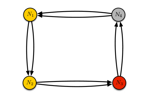
Figure 9: The BPS quiver of $\mathbb{F}_{0}$ theory. Yellow nodes and the arrows among them constitute the BPS quiver of $D=4$ theory. The red node carries the KK monopole charge while the gray one carries unit KK charge as well as negative of the KK monopole charge.

$\mathbb{F}_{1}\simeq dP_{1}$ geometry, which engineers $SU(2)_{\pi}$ theory, with a discrete theta angle associated to $\pi_{4}(SU(2))$ turned on, has the following map,

$$\begin{split}K[{\cal E}_{1}]=[\mathbf{E}_{0}]\,,\quad\qquad&\qquad\qquad\,K[{\cal E}_{2}]=-[\mathbf{E}_{0}]+[{\cal C}_{1}]\,,\\ K[{\cal E}_{3}]=-[\mathbf{E}_{0}]-[{\cal C}_{1}]&+[{\color[rgb]{1,0,0}{\cal C}_{2}}]\,,\quad K[{\cal E}_{4}]=[\mathbf{E}_{0}]-[{\color[rgb]{1,0,0}{\cal C}_{2}}]+[\text{pt}]\,.\end{split}$$ (B.3)

Its quiver is drawn in Figure 10.

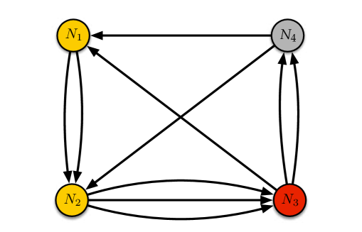
Figure 10: The BPS quiver of $\mathbb{F}_{1}$ theory.

$dP_{2}$ geometry renders the next map. This local CY engineers $D=5$ $SU(2)$ gauge theory with $N_{f}=1$ flavor. Its probe quiver is drawn in Figure 7.

$$\begin{split}K[{\cal E}_{1}]=[\mathbf{E}_{0}]\,,\quad K[{\cal E}_{2}]&=-[\mathbf{E}_{0}]+[{\cal C}_{3}]+[{\cal C}_{4}]\,,\quad K[{\cal E}_{3}]=-[{\cal C}_{3}]\,,\\ K[{\cal E}_{4}]=&-[\mathbf{E}_{0}]-[{\cal C}_{3}]-[{\cal C}_{4}]+[{\color[rgb]{1,0,0}{\cal C}_{5}}]\,,\\ K[{\cal E}_{5}]=&\,[\mathbf{E}_{0}]+[{\cal C}_{3}]-[{\color[rgb]{1,0,0}{\cal C}_{5}}]+[\text{pt}]\,.\end{split}$$ (B.4)

$dP_{3}$ theory makes the fifth table. This local CY engineers $D=5$ $SU(2)$ gauge theory with $N_{f}=2$ flavor.

$$\begin{split}K[{\cal E}_{1}]=[\mathbf{E}_{0}]\,,\,\,\,&\qquad K[{\cal E}_{2}]=-[\mathbf{E}_{0}]+[{\cal C}_{3}]+[{\cal C}_{4}]\,,\\ K[{\cal E}_{3}]=-[{\cal C}_{1}]\,,&\qquad K[{\cal E}_{4}]=-[{\cal C}_{3}]\,,\\ K[{\cal E}_{5}]=-[\mathbf{E}_{0}]&+[{\cal C}_{1}]+[{\color[rgb]{1,0,0}{\cal C}_{2}}]-[{\cal C}_{4}]\,,\\ K[{\cal E}_{6}]=[\mathbf{E}_{0}]&-[{\color[rgb]{1,0,0}{\cal C}_{2}}]+[\text{pt}]\,.\end{split}$$ (B.5)

Its quiver diagram is drawn in Figure 11.

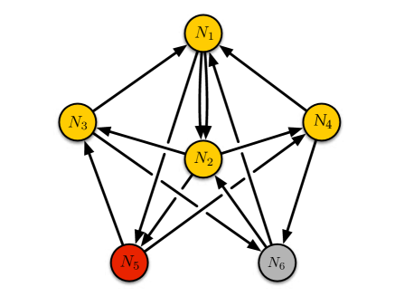
Figure 11: The quiver diagram of $dP_{3}$ theory.

The next theory we discuss is $Y^{3,q}$ family, which has $D=5$ ${\cal N}=1$ $SU(3)$ theory description. The integer label $q$ is interpreted as the Chern-Simons level of the gauge theory. Two examples of the probe quiver are illustrated in Figure 5 in Section 1. $Y^{3,0}$ theory has the map between internal cycles and fractional branes as follows.

$$\begin{split}K[{\cal E}_{1}]=[\mathbf{E}_{1}]\,,&\qquad K[{\cal E}_{2}]=-[\mathbf{E}_{1}]+[{\cal C}_{3}]\,,\\ K[{\cal E}_{3}]=[\mathbf{E}_{2}]\,,&\qquad K[{\cal E}_{4}]=-[\mathbf{E}_{2}]+[{\cal C}_{7}]\,,\\ K[{\cal E}_{5}]=-[\mathbf{E}_{1}]&-[\mathbf{E}_{2}]-[{\cal C}_{3}]-[{\cal C}_{7}]+[{\color[rgb]{1,0,0}{\cal C}_{9}}]\,,\\ K[{\cal E}_{6}]=[\mathbf{E}_{1}]&+[\mathbf{E}_{2}]-[{\color[rgb]{1,0,0}{\cal C}_{9}}]+[\text{pt}]\,.\end{split}$$ (B.6)

Another interesting theory of this class is $Y^{3,1}$, which engineers $D=5$ $SU(3)_{1}$ gauge theory.

$$\begin{split}K[{\cal E}_{1}]=[\mathbf{E}_{1}]\,,&\qquad K[{\cal E}_{2}]=-[\mathbf{E}_{1}]+[{\cal C}_{3}]\,,\\ K[{\cal E}_{3}]=[\mathbf{E}_{2}]\,,&\qquad K[{\cal E}_{4}]=-[\mathbf{E}_{2}]+[{\cal C}_{7}]\,,\\ K[{\cal E}_{5}]=-[\mathbf{E}_{1}]&-[\mathbf{E}_{2}]-[{\cal C}_{3}]-[{\cal C}_{7}]+[{\color[rgb]{1,0,0}{\cal C}_{9}}]\,,\\ K[{\cal E}_{6}]=[\mathbf{E}_{1}]&+[\mathbf{E}_{2}]-[{\color[rgb]{1,0,0}{\cal C}_{9}}]+[\text{pt}]\,.\end{split}$$ (B.7)

References

- [1] N. Seiberg, “Five dimensional SUSY field theories, non-trivial fixed points and string dynamics,” Phys. Lett. B 388 (1996), 753-760 [arXiv:hep-th/9608111 [hep-th]].
- [2] D. R. Morrison and N. Seiberg, “Extremal transitions and five-dimensional supersymmetric field theories,” Nucl. Phys. B 483 (1997), 229-247 [arXiv:hep-th/9609070 [hep-th]].
- [3] K. A. Intriligator, D. R. Morrison and N. Seiberg, “Five-dimensional supersymmetric gauge theories and degenerations of Calabi-Yau spaces,” Nucl. Phys. B 497 (1997), 56-100 [arXiv:hep-th/9702198 [hep-th]].
- [4] A. Klemm, W. Lerche, P. Mayr, C. Vafa and N. P. Warner, “Selfdual strings and N=2 supersymmetric field theory,” Nucl. Phys. B 477 (1996), 746-766 [arXiv:hep-th/9604034 [hep-th]].
- [5] S. H. Katz, A. Klemm and C. Vafa, “Geometric engineering of quantum field theories,” Nucl. Phys. B 497 (1997), 173-195 [arXiv:hep-th/9609239 [hep-th]].
- [6] N. Seiberg and E. Witten, “Electric - magnetic duality, monopole condensation, and confinement in N=2 supersymmetric Yang-Mills theory,” Nucl. Phys. B 426 (1994), 19-52 [erratum: Nucl. Phys. B 430 (1994), 485-486] [arXiv:hep-th/9407087 [hep-th]].
- [7] S. Kachru and M. Zimet, “A comment on 4d and 5d BPS states,” JHEP 01 (2020), 060 [arXiv:1808.01529 [hep-th]].
- [8] F. Denef, “Quantum quivers and Hall / hole halos,” JHEP 10 (2002), 023 [arXiv:hep-th/0206072 [hep-th]].
- [9] S. Lee and P. Yi, “Framed BPS States, Moduli Dynamics, and Wall-Crossing,” JHEP 04 (2011), 098 [arXiv:1102.1729 [hep-th]].
- [10] K. Hori, H. Kim and P. Yi, “Witten Index and Wall Crossing,” JHEP 01 (2015), 124 [arXiv:1407.2567 [hep-th]].
- [11] E. Witten, “Constraints on Supersymmetry Breaking,” Nucl. Phys. B 202 (1982), 253
- [12] E. Witten, “Phases of N=2 theories in two-dimensions,” AMS/IP Stud. Adv. Math. 1 (1996), 143-211 [arXiv:hep-th/9301042 [hep-th]].
- [13] J. M. Maldacena, A. Strominger and E. Witten, “Black hole entropy in M theory,” JHEP 12 (1997), 002 [arXiv:hep-th/9711053 [hep-th]].
- [14] A. Gadde, S. Gukov and P. Putrov, “Fivebranes and 4-manifolds,” Prog. Math. 319, 155-245 (2016) [arXiv:1306.4320 [hep-th]].
- [15] C. Closset and M. Del Zotto, “On 5d SCFTs and their BPS quivers. Part I: B-branes and brane tilings,” [arXiv:1912.13502 [hep-th]].
- [16] B. Feng, A. Hanany and Y. H. He, “D-brane gauge theories from toric singularities and toric duality,” Nucl. Phys. B 595 (2001), 165-200 [arXiv:hep-th/0003085 [hep-th]].
- [17] A. Hanany and K. D. Kennaway, “Dimer models and toric diagrams,” [arXiv:hep-th/0503149 [hep-th]].
- [18] S. Franco, A. Hanany, K. D. Kennaway, D. Vegh and B. Wecht, “Brane dimers and quiver gauge theories,” JHEP 01 (2006), 096 [arXiv:hep-th/0504110 [hep-th]].
- [19] A. Hanany, C. P. Herzog and D. Vegh, “Brane tilings and exceptional collections,” JHEP 07 (2006), 001 [arXiv:hep-th/0602041 [hep-th]].
- [20] M. R. Douglas and G. W. Moore, “D-branes, quivers, and ALE instantons,” [arXiv:hep-th/9603167 [hep-th]].
- [21] M. R. Douglas, B. R. Greene and D. R. Morrison, “Orbifold resolution by D-branes,” Nucl. Phys. B 506 (1997), 84-106 [arXiv:hep-th/9704151 [hep-th]]
- [22] C. Beasley, B. R. Greene, C. I. Lazaroiu and M. R. Plesser, “D3-branes on partial resolutions of Abelian quotient singularities of Calabi-Yau threefolds,” Nucl. Phys. B 566 (2000), 599-640 [arXiv:hep-th/9907186 [hep-th]].
- [23] J. P. Gauntlett, D. Martelli, J. Sparks and D. Waldram, “Sasaki-Einstein metrics on ,” Adv. Theor. Math. Phys. 8 (2004) no.4, 711-734 [arXiv:hep-th/0403002 [hep-th]].
- [24] S. Benvenuti, S. Franco, A. Hanany, D. Martelli and J. Sparks, “An Infinite family of superconformal quiver gauge theories with Sasaki-Einstein duals,” JHEP 06 (2005), 064 [arXiv:hep-th/0411264 [hep-th]].
- [25] D. Martelli and J. Sparks, “Toric Sasaki-Einstein metrics on ,” Phys. Lett. B 621 (2005), 208-212 [arXiv:hep-th/0505027 [hep-th]].
- [26] A. Hanany, P. Kazakopoulos and B. Wecht, “A New infinite class of quiver gauge theories,” JHEP 08 (2005), 054 [arXiv:hep-th/0503177 [hep-th]].
- [27] S. J. Lee and P. Yi, “Witten Index for Noncompact Dynamics,” JHEP 06 (2016), 089 [arXiv:1602.03530 [hep-th]].
- [28] M. F. Atiyah, V. Patodi, and I. Singer, “Spectral asymmetry and Riemannian geometry,” Bull. London Math. Soc 5 (1973), no. 2 229-234.
- [29] S. J. Lee, Z. L. Wang and P. Yi, “BPS States, Refined Indices, and Quiver Invariants,” JHEP 1210 (2012) 094 [arXiv:1207.0821 [hep-th]].
- [30] SageMath, the Sage Mathematics Software System (Version 9.1), The Sage Developers, https://www.sagemath.org (2020).
- [31] T. Hausel, E. Hunsicker and R. Mazzeo, “Hodge cohomology of gravitational instantons,” [arXiv:math/0207169 [math.DG]].
- [32] I. Macdonald, “The Poincaré Polynomial of a Symmetric Product,” Mathematical Proceedings of the Cambridge Philosophical Society, 58(4), 563-568.
- [33] P. Yi, “Witten index and threshold bound states of D-branes,” Nucl. Phys. B 505 (1997) 307 [hep-th/9704098].
- [34] S. Sethi and M. Stern, “D-brane bound states redux,” Commun. Math. Phys. 194 (1998) 675 [hep-th/9705046].
- [35] G. W. Moore, N. Nekrasov and S. Shatashvili, “D particle bound states and generalized instantons,” Commun. Math. Phys. 209 (2000), 77-95 [arXiv:hep-th/9803265 [hep-th]].
- [36] M. B. Green and M. Gutperle, “D Particle bound states and the D instanton measure,” JHEP 01 (1998), 005 [arXiv:hep-th/9711107 [hep-th]].
- [37] V. G. Kac and A. V. Smilga, “Normalized vacuum states in N=4 supersymmetric Yang-Mills quantum mechanics with any gauge group,” Nucl. Phys. B 571 (2000), 515-554 [arXiv:hep-th/9908096 [hep-th]].
- [38] E. Witten, “String theory dynamics in various dimensions,” Nucl. Phys. B 443 (1995), 85-126 [arXiv:hep-th/9503124 [hep-th]].
- [39] J. Polchinski, “M theory and the light cone,” Prog. Theor. Phys. Suppl. 134 (1999), 158-170 [arXiv:hep-th/9903165 [hep-th]].
- [40] J. Manschot, B. Pioline and A. Sen, “Wall Crossing from Boltzmann Black Hole Halos,” JHEP 07 (2011), 059 [arXiv:1011.1258 [hep-th]].
- [41] H. Kim, J. Park, Z. Wang and P. Yi, “Ab Initio Wall-Crossing,” JHEP 09 (2011), 079 [arXiv:1107.0723 [hep-th]].
- [42] J. Manschot, B. Pioline and A. Sen, “On the Coulomb and Higgs branch formulae for multi-centered black holes and quiver invariants,” JHEP 05 (2013), 166 [arXiv:1302.5498 [hep-th]].
- [43] J. Manschot, B. Pioline and A. Sen, “The Coulomb Branch Formula for Quiver Moduli Spaces,” [arXiv:1404.7154 [hep-th]].
- [44] S. -J. Lee, Z. -L. Wang and P. Yi, “Quiver invariants from intrinsic Higgs states,” JHEP 1207 (2012), 169 [arXiv:1205.6511 [hep-th]].
- [45] M. Kontsevich and Y. Soibelman, “Stability structures, motivic Donaldson-Thomas invariants and cluster transformations,” [arXiv:0811.2435 [math.AG]].
- [46] A. Sen, “Equivalence of three wall-crossing formulae,” Commun. Num. Theor. Phys. 6 (2012), 601-659 [arXiv:1112.2515 [hep-th]].
- [47] I. Bena, M. Berkooz, J. de Boer, S. El-Showk and D. Van den Bleeken, “Scaling BPS Solutions and pure-Higgs States,” JHEP 1211 (2012), 171 [arXiv:1205.5023 [hep-th]].
- [48] F. Denef and G. W. Moore, “Split states, entropy enigmas, holes and halos,” JHEP 11 (2011), 129 [arXiv:hep-th/0702146 [hep-th]].
- [49] G. Beaujard, J. Manschot and B. Pioline, “Vafa-Witten invariants from exceptional collections,” [arXiv:2004.14466 [hep-th]].
- [50] D. Bak, C. K. Lee, K. M. Lee and P. Yi, “Low-energy dynamics for 1/4 BPS dyons,” Phys. Rev. D 61 (2000), 025001 [arXiv:hep-th/9906119 [hep-th]].
- [51] J. P. Gauntlett, C. J. Kim, K. M. Lee and P. Yi, “General low-energy dynamics of supersymmetric monopoles,” Phys. Rev. D 63 (2001), 065020 [arXiv:hep-th/0008031 [hep-th]].
- [52] M. Stern and P. Yi, “Counting Yang-Mills dyons with index theorems,” Phys. Rev. D 62 (2000), 125006 [arXiv:hep-th/0005275 [hep-th]].
- [53] K. M. Lee and P. Yi, “Monopoles and instantons on partially compactified D-branes,” Phys. Rev. D 56 (1997), 3711-3717 [arXiv:hep-th/9702107 [hep-th]].
- [54] C. Fraser and T. J. Hollowood, “On the weak coupling spectrum of N=2 supersymmetric SU(n) gauge theory,” Nucl. Phys. B 490 (1997), 217-238 [arXiv:hep-th/9610142 [hep-th]].
- [55] M. Alim, S. Cecotti, C. Cordova, S. Espahbodi, A. Rastogi and C. Vafa, “ quantum field theories and their BPS quivers,” Adv. Theor. Math. Phys. 18 (2014) no.1, 27-127 [arXiv:1112.3984 [hep-th]].
- [56] K. M. Lee, “Instantons and magnetic monopoles on with arbitrary simple gauge groups,” Phys. Lett. B 426 (1998), 323-328 [arXiv:hep-th/9802012 [hep-th]].
- [57] P. Bousseau, “Scattering diagrams, stability conditions, and coherent sheaves on ,” [arXiv:1909.02985 [math.AG]].
- [58] K. Behrend, J. Bryan and B. Szendroi, “Motivic degree zero Donaldson-Thomas invariants,” [arXiv:0909.5088 [math.AG]].
- [59] A. Morrison, S. Mozgovoy, K. Nagao and B. Szendroi, “Motivic Donaldson-Thomas invariants of the conifold and the refined topological vertex,” [arXiv:1107.5017 [math.AG]].
- [60] A. Morrison and K. Nagao, “Motivic Donaldson-Thomas invariants of toric small crepant resolutions,” Algebra Number Theory 9 (2015) no.4, 767-813 [arXiv:1110.5976 [math.AG]].
- [61] S. Banerjee, P. Longhi and M. Romo, “Exploring 5d BPS Spectra with Exponential Networks,” Annales Henri Poincare 20 (2019) no.12, 4055-4162 [arXiv:1811.02875 [hep-th]].
- [62] S. Banerjee, P. Longhi and M. Romo, “Exponential BPS graphs and D brane counting on toric Calabi-Yau threefolds: Part I,” [arXiv:1910.05296 [hep-th]].
- [63] G. Bonelli, F. Del Monte and A. Tanzini, “BPS quivers of five-dimensional SCFTs, Topological Strings and q-Painlevé equations,” [arXiv [hep-th]].