Fully-heavy pentaquark states

Abstract

Developing the calculation techniques to fivefold heavy hadrons, we perform the study of novel fully-heavy $QQQQ\bar{Q}$ pentaquark states by the QCD sum rule approach that is firmly based on the QCD basic theory. Numerically, masses of fully-heavy pentaquark states are calculated to be $7.41^{+0.27}_{-0.31}~{}\mbox{GeV}$ for $cccc\bar{c}$ and $21.60^{+0.73}_{-0.22}~{}\mbox{GeV}$ for $bbbb\bar{b}$, respectively. In experiment, these predicted all-heavy pentaquark states could be searched for in the $\Omega_{QQQ}\eta_{Q}$ invariant mass spectrum.

I Introduction

In recent years, hunting for evidences of the multiquark states composed of more than three quarks have attracted one’s great interest. Not long ago, LHCb Collaboration observed a broad structure just above twice the $J/\psi$ mass and a narrower structure $X(6900)$ by using proton-proton collision data, for which could possibly be all-charmed tetraquark states LHCb . Before this, LHCb Collaboration discovered a narrow state $P_{c}(4312)^{+}$ in the $J/\psi p$ invariant mass spectrum, and separated the formerly reported $P_{c}(4450)^{+}$ LHCb-1 to two narrow overlapping peaks, $P_{c}(4440)^{+}$ and $P_{c}(4457)^{+}$, for which could be some pentaquark state candidates LHCb-2 . On the investigations of these exotic states, there are actually large numbers of related works and one could see some recent reviews rev-1 ; rev-2 ; rev-3 ; rev-4 ; rev-5 ; rev-6 ; rev-7 ; rev-8 and references therein. In addition, there newly appeared a systematical study on the mass spectra of ground pentaquark states in a modified chromo-magnetic interaction model Liu . Making a synthetical consideration of all these observations, it seems very promising that pentaquark states consist of fully-charmed quarks could be found in the $\Omega_{ccc}\eta_{c}$ invariant mass spectrum experimentally.

Without any light quark contamination, fully-heavy pentaquark states are quite ideal prototypes to refine one’s knowledge on heavy quark dynamics. To probe a fully-heavy pentaquark state, one inevitably has to confront the very intricate nonperturbative QCD problem. As one reliable way for calculating nonperturbative effects, the QCD sum rule svzsum is firmly founded on the QCD theory, and has been successfully applied to plenty of hadronic states overview ; overview1 ; overview2 ; overview3 . Referring to fully-heavy pentaquark states, the related operator product expansion (OPE) calculations are quite complicated as one has to treat many multi-loop massive propagator diagrams. Making the development of corresponding calculation techniques, we devote to investigating fully-heavy pentaquark states with the help of trustworthy QCD sum rule method in this paper.

The rest of the paper is organized as below. The QCD sum rule is derived for fully-heavy pentaquark states in Sec. II, followed by numerical analysis and discussions in Sec. III. The last part presents a brief summary.

II Fully-heavy pentaquark states in QCD sum rules

Consulting interpolating currents for heavy mesons reinders and baryons Ioffe in full QCD, one can construct the following form of current

$$j_{\mu}=(\epsilon_{abc}Q_{a}^{T}C\gamma_{\mu}Q_{b}Q_{c})(Q_{e}i\gamma_{5}\bar{Q}_{e}),$$ (1)

for $QQQQ\bar{Q}$ pentaquark states. Here $T$ denotes matrix transposition, $C$ means the charge conjugation matrix, $Q$ could be the heavy charm or bottom quark, and the subscript $a$, $b$, $c$, and $e$ are color indices.

Generally, the two-point correlator

$$\Pi_{\mu\nu}(q^{2})=i\int d^{4}x\mbox{e}^{iq.x}\langle 0|T[j_{\mu}(x)\overline{j_{\nu}}(0)]|0\rangle,$$ (2)

can be parameterized as

$$\Pi_{\mu\nu}(q^{2})=-g_{\mu\nu}[\not{q}\Pi_{1}(q^{2})+\Pi_{2}(q^{2})]+....$$ (3)

Concerning with the part proportional to $-g_{\mu\nu}\not{q}$, matching its descriptions at the hadron level and at the quark level, and applying a Borel transform, one arrives at

$$\lambda^{2}e^{-M_{H}^{2}/M^{2}} = \int_{25m_{Q}^{2}}^{s_{0}}ds\rho e^{-s/M^{2}},$$ (4)

in which $M_{H}$ is the studied hadron’s mass and the spectral density $\rho=\frac{1}{\pi}\mbox{Im}\Pi_{1}(s)$. Taking the derivative of Eq. (4) with respect to $-\frac{1}{M^{2}}$ and then dividing the result by Eq. (4) itself, one could acquire the mass

$$M_{H} = \sqrt{\int_{25m_{Q}^{2}}^{s_{0}}ds\rho se^{-s/M^{2}}/\int_{25m_{Q}^{2}}^{s_{0}}ds\rho e^{-s/M^{2}}}.$$ (5)

In the OPE calculation, one works at the momentum-space with the heavy-quark propagator reinders , and then the result is dimensionally regularized at $D=4$, by extending the interrelated techniques Nielsen ; Zhang to fully-heavy pentaquark systems. Concretely, the spectral density $\rho=\rho^{\mbox{pert}}+\rho^{\langle g^{2}G^{2}\rangle}+\rho^{\langle g^{3}G^{3}\rangle}$ is expressed as

$$\rho^{\mbox{pert}} = \frac{3}{5\cdot 2^{14}\pi^{8}}\int_{\alpha_{min}}^{\alpha_{max}}\frac{d\alpha}{\alpha^{3}}\int_{\beta_{min}}^{\beta_{max}}\frac{d\beta}{\beta^{3}}\int_{\gamma_{min}}^{\gamma_{max}}\frac{d\gamma}{\gamma^{3}}\int_{\xi_{min}}^{\xi_{max}}\frac{d\xi}{\xi^{3}}\frac{\textbf{h}^{3}(m_{Q}^{2}-\textbf{h}s)^{3}}{(1-\alpha-\beta-\gamma-\xi)^{3}}\bigg{[}-8\textbf{h}^{2}(m_{Q}^{2}-\textbf{h}s)^{2}$$

$$+ (35\textbf{h}^{3}s+25\alpha\beta\textbf{h}m_{Q}^{2})(m_{Q}^{2}-\textbf{h}s)-20\textbf{h}^{4}s^{2}-40\alpha\beta\textbf{h}^{2}m_{Q}^{2}s-20\alpha\beta\gamma\xi m_{Q}^{4}\bigg{]},$$

$$\rho^{\langle g^{2}G^{2}\rangle} = \frac{m_{Q}^{2}\langle g^{2}G^{2}\rangle}{2^{14}\pi^{8}}\int_{\alpha_{min}}^{\alpha_{max}}\frac{d\alpha}{\alpha^{3}}\int_{\beta_{min}}^{\beta_{max}}\frac{d\beta}{\beta^{3}}\int_{\gamma_{min}}^{\gamma_{max}}\frac{d\gamma}{\gamma^{3}}\int_{\xi_{min}}^{\xi_{max}}\frac{d\xi}{\xi^{3}}\frac{\textbf{h}^{3}}{(1-\alpha-\beta-\gamma-\xi)^{3}}\bigg{\{}\Big{[}(1-\alpha-\beta$$

$$- \gamma-\xi)^{3}+2\beta^{3}+2\xi^{3}\Big{]}\Big{[}-4\textbf{h}^{2}(m_{Q}^{2}-\textbf{h}s)^{2}+7\textbf{h}^{3}s(m_{Q}^{2}-\textbf{h}s)-\textbf{h}^{4}s^{2}-\alpha\beta\gamma\xi m_{Q}^{4}+3\alpha\beta\textbf{h}m_{Q}^{4}$$

$$- 4\alpha\beta\textbf{h}^{2}m_{Q}^{2}s\Big{]}+\alpha\beta(1-\alpha-\beta-\gamma-\xi)^{3}\textbf{h}m_{Q}^{2}(2m_{Q}^{2}-3\textbf{h}s)+2\gamma\xi(\beta^{3}+\xi^{3})\textbf{h}m_{Q}^{2}(2m_{Q}^{2}-3\textbf{h}s)$$

$$- 6\alpha\beta\gamma\xi(\beta^{2}+\xi^{2})m_{Q}^{2}(m_{Q}^{2}-\textbf{h}s)-6(\gamma\xi^{3}+\alpha\beta^{3})\textbf{h}^{2}s(m_{Q}^{2}-\textbf{h}s)+3\textbf{h}(3\alpha\beta^{3}+2\gamma\xi^{3})(m_{Q}^{2}-\textbf{h}s)^{2}\bigg{\}},$$

and

$$\rho^{\langle g^{3}G^{3}\rangle} = \frac{\langle g^{3}G^{3}\rangle}{2^{16}\pi^{8}}\int_{\alpha_{min}}^{\alpha_{max}}\frac{d\alpha}{\alpha^{3}}\int_{\beta_{min}}^{\beta_{max}}\frac{d\beta}{\beta^{3}}\int_{\gamma_{min}}^{\gamma_{max}}\frac{d\gamma}{\gamma^{3}}\int_{\xi_{min}}^{\xi_{max}}\frac{d\xi}{\xi^{3}}\frac{\textbf{h}^{3}}{(1-\alpha-\beta-\gamma-\xi)^{3}}\bigg{\{}\Big{[}(1-\alpha-\beta-\gamma-\xi)^{3}$$

$$+ 2\beta^{3}+2\xi^{3}\Big{]}\Big{[}-4\textbf{h}^{2}(m_{Q}^{2}-\textbf{h}s)^{2}+7\textbf{h}^{3}s(m_{Q}^{2}-\textbf{h}s)-\textbf{h}^{4}s^{2}\Big{]}+2\alpha\beta\Big{[}(1-\alpha-\beta-\gamma-\xi)^{3}+6\beta^{3}+\xi^{3}\Big{]}$$

$$\times \textbf{h}m_{Q}^{2}(3m_{Q}^{2}-4\textbf{h}s)-\alpha\beta\gamma\xi\Big{[}(1-\alpha-\beta-\gamma-\xi)^{3}+12\beta^{3}+12\xi^{3}\Big{]}m_{Q}^{4}-\alpha\beta(1-\alpha-\beta-\gamma-\xi)^{3}$$

$$\times \textbf{h}m_{Q}^{2}(m_{Q}^{2}-\textbf{h}s)+2\gamma\xi(\beta^{3}+6\xi^{3})\textbf{h}m_{Q}^{2}(2m_{Q}^{2}-3\textbf{h}s)-2\Big{[}(1-\alpha-\beta-\gamma-\xi)^{4}+2\beta^{4}+2\xi^{4}\Big{]}$$

$$\times \textbf{h}^{2}m_{Q}^{2}(8m_{Q}^{2}-15\textbf{h}s)+2\textbf{h}m_{Q}^{4}\Big{[}5\alpha\beta(1-\alpha-\beta-\gamma-\xi)^{4}+2(3\alpha\beta+2\gamma\xi)(\beta^{4}+\xi^{4})\Big{]}\bigg{\}}.$$

It is defined as $\textbf{h}=\frac{1}{\frac{1}{\alpha}+\frac{1}{\beta}+\frac{1}{\gamma}+\frac{1}{\xi}+\frac{1}{1-\alpha-\beta-\gamma-\xi}}$, and the integration limits of $\alpha$, $\beta$, $\gamma$, and $\xi$ are given by

$$\alpha = \frac{1}{2}\Bigg{[}\bigg{(}1-\frac{15m_{Q}^{2}}{s}\bigg{)}\pm\sqrt{\bigg{(}1-\frac{15m_{Q}^{2}}{s}\bigg{)}^{2}-\frac{4m_{Q}^{2}}{s}}\Bigg{]},$$

$$\beta = \frac{1}{2}\Bigg{[}\Big{(}1-\alpha-\frac{8\alpha m_{Q}^{2}}{\alpha s-m_{Q}^{2}}\Big{)}\pm\sqrt{\Big{(}1-\alpha-\frac{8\alpha m_{Q}^{2}}{\alpha s-m_{Q}^{2}}\Big{)}^{2}-\frac{4\alpha(1-\alpha)m_{Q}^{2}}{\alpha s-m_{Q}^{2}}}\Bigg{]},$$

$$\gamma = \frac{1}{2}\Bigg{[}\Big{(}1-\alpha-\beta-\frac{3}{\frac{s}{m_{Q}^{2}}-\frac{1}{\alpha}-\frac{1}{\beta}}\Big{)}\pm\sqrt{\Big{(}1-\alpha-\beta-\frac{3}{\frac{s}{m_{Q}^{2}}-\frac{1}{\alpha}-\frac{1}{\beta}}\Big{)}^{2}-4\frac{1-\alpha-\beta}{\frac{s}{m_{Q}^{2}}-\frac{1}{\alpha}-\frac{1}{\beta}}}\Bigg{]},$$

and

$$\xi = \frac{1}{2}\Bigg{[}\Big{(}1-\alpha-\beta-\gamma\Big{)}\pm\sqrt{\Big{(}1-\alpha-\beta-\gamma\Big{)}^{2}-4\frac{1-\alpha-\beta-\gamma}{\frac{s}{m_{Q}^{2}}-\frac{1}{\alpha}-\frac{1}{\beta}-\frac{1}{\gamma}}}\Bigg{]}.$$

As the usual QCD sum rule treatment, it mainly takes into account the well-known two-gluon condensate $\langle g^{2}G^{2}\rangle$ and three-gluon condensate $\langle g^{3}G^{3}\rangle$ here. Note that it was discussed that including higher-dimension gluonic condensates may be helpful to the sum rule analysis to some extent. In that case, those higher-dimension gluonic operators would require some speculative input assumptions for their numerical values. Generally speaking, the higher the dimension of the gluonic operator, the less known the value of its matrix element. By way of parenthesis, involving those unascertained higher dimensional gluonic condensates, one technically has to accomplish a tremendous task since a number of multi-loop massive propagator diagrams need to be treated for the present fully-heavy pentaquark states, for which could be taken into account in some further work.

III Numerical analysis and discussions

The input parameters are taken as $\langle g^{2}G^{2}\rangle=0.88\pm 0.25~{}\mbox{GeV}^{4}$ and $\langle g^{3}G^{3}\rangle=0.58\pm 0.18~{}\mbox{GeV}^{6}$ svzsum ; overview3 ; Narison , and $m_{Q}$ is set as the running charm mass $m_{c}=1.27\pm 0.02~{}\mbox{GeV}$ PDG at first. As one knows, the QCD sum rule method has made approximations in the OPE of the correlation functions and introduced a very complicated and largely unknown structure of the hadronic dispersion integrals in the phenomenological side. In this way, complying with the criterion of sum rule analysis, one should find appropriate work windows for both the continuum threshold $\sqrt{s_{0}}$ and the Borel parameter $M^{2}$ in which the two sides of QCD sum rules have a good overlap and information on the hadronic resonance can be reliably extracted. In phenomenology, the threshold $\sqrt{s_{0}}$ is the energy which characterizes the beginning of the continuum state and the gap $\sqrt{s_{0}}-M_{H}$ is typically evaluated to be about $0.3\sim 0.8~{}\mbox{GeV}$ overview3 . Meanwhile, the proper Borel window of $M^{2}$ can be found by analyzing the OPE convergence and the pole dominance: the lower value of $M^{2}$ is obtained by considering the OPE convergence, and the upper one of $M^{2}$ is get from the condition that the pole contribution should be bigger than the continuum contribution.

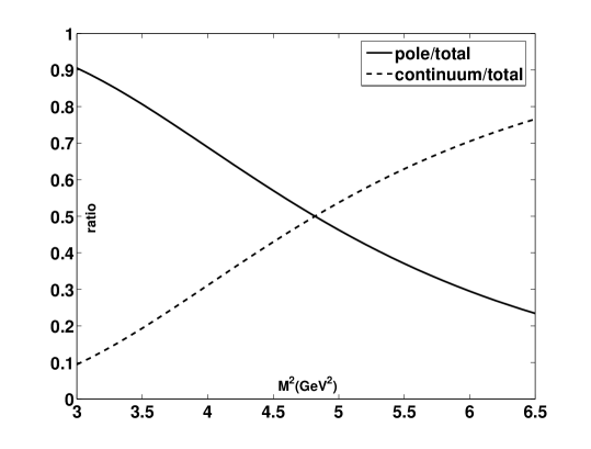
At the start, the input parameters are kept at their central values. The OPE convergence for the $cccc\bar{c}$ pentaquark state can be analyzed by comparing the relative contributions of various condensates from sum rule (4). It is noted that the three-gluon condensate $\langle g^{3}G^{3}\rangle$ with dimension six is much smaller than two-gluon condensate $\langle g^{2}G^{2}\rangle$ or perturbative contribution. In view of the OPE convergence analysis, the lower bound of $M^{2}$ is numerically taken as $M^{2}\geq 3.5~{}\mbox{GeV}^{2}$. Phenomenologically, one could fix the upper bound of $M^{2}$ according to the pole dominance requirement. For example, by making the comparison between pole and continuum contribution from sum rule (4) for $\sqrt{s_{0}}=8.0~{}\mbox{GeV}$ in FIG. 1, one notes that the relative pole contribution is around $50\%$ at $M^{2}=4.8~{}\mbox{GeV}^{2}$ and it descends with $M^{2}$. Accordingly, the pole dominance condition could be satisfied when $M^{2}\leq 4.8~{}\mbox{GeV}^{2}$, and the Borel window is chosen as $M^{2}=3.5\sim 4.8~{}\mbox{GeV}^{2}$ for $\sqrt{s_{0}}=8.0~{}\mbox{GeV}$. With an eye to the typical gap between the continuum and resonance, the variation of threshold $\sqrt{s_{0}}$ is taken as $\sqrt{s_{0}}=7.7\sim 8.2~{}\mbox{GeV}$ for $cccc\bar{c}$. By way of the similar analysis as above, the corresponding Borel windows are fixed as $M^{2}=3.5\sim 4.1~{}\mbox{GeV}^{2}$ for $\sqrt{s_{0}}=7.7~{}\mbox{GeV}$, and $M^{2}=3.5\sim 5.3~{}\mbox{GeV}^{2}$ for $\sqrt{s_{0}}=8.2~{}\mbox{GeV}$, respectively.

Figure 1: The phenomenological contribution in sum rule (4) for $\sqrt{s_{0}}=8.0~{}\mbox{GeV}$ for the fully-heavy $cccc\bar{c}$ pentaquark state. The solid line is the relative pole contribution as a function of $M^{2}$ and the dashed line is the relative continuum contribution.

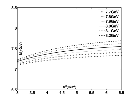
The Borel curves for the $cccc\bar{c}$ pentaquark state are shown in FIG. 2, and in the chosen work windows its mass is extracted to be $7.41^{+0.20}_{-0.23}~{}\mbox{GeV}$. After varying the input parameters, the achieved mass is $7.41^{+0.20+0.07}_{-0.23-0.08}~{}\mbox{GeV}$ (the first uncertainty from the variation of threshold $\sqrt{s_{0}}$ and the Borel parameter $M^{2}$, and the second one due to the uncertainty of QCD parameters) or compactly $7.41^{+0.27}_{-0.31}~{}\mbox{GeV}$.

Figure 2: The mass $M_{H}$ dependence on $M^{2}$ for the fully-heavy $cccc\bar{c}$ pentaquark state from sum rule (5) is shown. The Borel windows of $M^{2}$ are $3.5\sim 4.1~{}\mbox{GeV}^{2}$ for $\sqrt{s_{0}}=7.7~{}\mbox{GeV}$, $3.5\sim 4.8~{}\mbox{GeV}^{2}$ for $\sqrt{s_{0}}=8.0~{}\mbox{GeV}$, and $3.5\sim 5.3~{}\mbox{GeV}^{2}$ for $\sqrt{s_{0}}=8.2~{}\mbox{GeV}$, respectively.

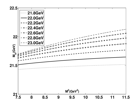
Replacing the heavy $m_{Q}$ by the running bottom mass $m_{b}=4.18_{-0.02}^{+0.03}~{}\mbox{GeV}$ PDG , one could straightway put forward the corresponding analysis for fully-bottomed $bbbb\bar{b}$ pentaquark state. Considering the much bigger mass of $bbbb\bar{b}$, the typical gap may be somewhat small for the fully-heavy $bbbb\bar{b}$ pentaquark state. Thus, the gap has been further broadened and the associated theoretical uncertainty has been included to give a conservative mass prediction for $bbbb\bar{b}$. Correspondingly, the threshold $\sqrt{s_{0}}$ for $bbbb\bar{b}$ is varied as $21.8\sim 23.0~{}\mbox{GeV}$, and its Borel curves are displayed in FIG. 3. Having taken into the uncertainty of both work windows and QCD parameters, the mass value is computed to be $21.60^{+0.73}_{-0.22}~{}\mbox{GeV}$ for the $bbbb\bar{b}$ pentaquark state.

Figure 3: The mass $M_{H}$ dependence on $M^{2}$ for the fully-heavy $bbbb\bar{b}$ pentaquark state from sum rule (5) is shown. The Borel windows of $M^{2}$ are $8.0\sim 8.4~{}\mbox{GeV}^{2}$ for $\sqrt{s_{0}}=21.8~{}\mbox{GeV}$, $8.0\sim 9.6~{}\mbox{GeV}^{2}$ for $\sqrt{s_{0}}=22.0~{}\mbox{GeV}$, $8.0\sim 11.0~{}\mbox{GeV}^{2}$ for $\sqrt{s_{0}}=22.2~{}\mbox{GeV}$, and $8.0\sim 11.5~{}\mbox{GeV}^{2}$ for $\sqrt{s_{0}}=23.0~{}\mbox{GeV}$, respectively.

IV Summary

By making the development of calculation techniques to fivefold heavy pentaquark states, we present the investigation of fully-heavy $QQQQ\bar{Q}$ pentaquark states from trustable QCD sum rules. Eventually, their mass spectrums are predicted to be $7.41^{+0.27}_{-0.31}~{}\mbox{GeV}$ for the $cccc\bar{c}$ state, and $21.60^{+0.73}_{-0.22}~{}\mbox{GeV}$ for the $bbbb\bar{b}$ state, respectively. It is proposed that these states could be experimentally looked for in the $\Omega_{QQQ}\eta_{Q}$ invariant mass spectrum. For the future, one can expect that further theoretical studies and experimental efforts may shed more light on the nature of exotic fully-heavy pentaquark states.

References

• (1) R. Aaij et al. (LHCb Collaboration), Sci. Bull. 65, 1983 (2020).
• (2) R. Aaij et al. (LHCb Collaboration), Phys. Rev. Lett. 115, 072001 (2015).
• (3) R. Aaij et al. (LHCb Collaboration), Phys. Rev. Lett. 122, 222001 (2019).
• (4) H. X. Chen, W. Chen, X. Liu, and S. L. Zhu, Phys. Rept. 639, 1 (2016).
• (5) A. Esposito, A. Pilloni, and A. D. Polosa, Phys. Rept. 668, 1 (2016).
• (6) A. Ali, J. S. Lange, and S. Stone, Prog. Part. Nucl. Phys. 97, 123 (2017).
• (7) R. F. Lebed, R. E. Mitchell, and E. S. Swanson, Prog. Part. Nucl. Phys. 93, 143 (2017).
• (8) F. K. Guo, C. Hanhart, U. G. Meissner, Q. Wang, Q. Zhao, and B. S. Zou, Rev. Mod. Phys. 90, 015004 (2018).
• (9) Y. R. Liu, H. X. Chen, W. Chen, X. Liu, and S. L. Zhu, Prog. Part. Nucl. Phys. 107, 237 (2019).
• (10) N. Brambilla, S. Eidelman, C. Hanhart, A. Nefediev, C. P. Shen, C. E. Thomas, A. Vairo, and C. Z. Yuan, Phys. Rept. 873, 1 (2020).
• (11) G. Yang, J. L. Ping, and J. Segovia, arXiv:2009.00238 [hep-ph].
• (12) H. T. An, K. Chen, and X. Liu, arXiv:2010.05014 [hep-ph].
• (13) M. A. Shifman, A. I. Vainshtein, and V. I. Zakharov, Nucl. Phys. B147, 385 (1979); B147, 448 (1979); V. A. Novikov, M. A. Shifman, A. I. Vainshtein, and V. I. Zakharov, Fortschr. Phys. 32, 585 (1984).
• (14) B. L. Ioffe, in The Spin Structure of The Nucleon, edited by B. Frois, V. W. Hughes, and N. de Groot (World Scientific, Singapore, 1997).
• (15) S. Narison, Camb. Monogr. Part. Phys. Nucl. Phys. Cosmol. 17, 1 (2002), arXiv:hep-ph/0205006.
• (16) P. Colangelo and A. Khodjamirian, in At the Frontier of Particle Physics: Handbook of QCD, edited by M. Shifman, Boris Ioffe Festschrift Vol. 3 (World Scientific, Singapore, 2001), pp. 1495-1576.
• (17) M. Nielsen, F. S. Navarra, and S. H. Lee, Phys. Rep. 497, 41 (2010).
• (18) L. J. Reinders, H. R. Rubinstein, and S. Yazaki, Phys. Rep. 127, 1 (1985).
• (19) B. L. Ioffe, Nucl. Phys. B188, 317 (1981); E. V. Shuryak, Nucl. Phys. B198, 83 (1982).
• (20) H. Kim and Y. Oh, Phys. Rev. D 72, 074012 (2005); M. E. Bracco, A. Lozea, R. D. Matheus, F. S. Navarra, and M. Nielsen, Phys. Lett. B 624, 217 (2005); R. D. Matheus, S. Narison, M. Nielsen, and J. M. Richard, Phys. Rev. D 75, 014005 (2007).
• (21) J. R. Zhang and M. Q. Huang, Phys. Lett. B 674, 28 (2009); J. R. Zhang, Phys. Rev. D 87, 076008 (2013); Phys. Rev. D 89, 096006 (2014); Phys. Rev. D 103, 014018 (2021).
• (22) S. Narison, Phys. Rep. 84, 263 (1982); G. Launer, S. Narison, and R. Tarrach, Z. Phys. C 26, 433 (1984); S. Narison, Phys. Lett. B 673, 30 (2009).
• (23) M. Tanabashi et al. (Particle Data Group), Phys. Rev. D 98, 030001 (2018) and 2019 update.