Absorption-selected galaxies trace the low-mass, late-type, star-forming population at $z\sim 2-3$

Abstract

We report on the stellar content, half-light radii and star formation rates of a sample of 10 known high-redshift ($z\gtrsim 2$) galaxies selected on strong neutral hydrogen (H i) absorption ($\log({\rm N_{H\,\textsc{i}}\>/\>cm}^{-2})>19$) toward background quasars. We use observations from the Hubble Space Telescope (HST) Wide Field Camera 3 in three broad-band filters to study the spectral energy distribution (SED) of the galaxies. Using careful quasar point spread function subtraction, we study their galactic environments, and perform the first systematic morphological characterisation of such absorption-selected galaxies at high redshifts. Our analysis reveals complex, irregular hosts with multiple star-forming clumps. At a spatial sampling of 0.067 arcsec per pixel (corresponding to 0.55 kpc at the median redshift of our sample), 40% of our sample requires multiple Sérsic components for an accurate modelling of the observed light distributions. Placed on the mass–size relation and the ‘main sequence’ of star-forming galaxies, we find that absorption-selected galaxies at high redshift extend known relations determined from deep luminosity-selected surveys to an order of magnitude lower stellar mass, with objects primarily composed of star-forming, late-type galaxies. We measure half-light radii in the range $r_{1/2}\sim 0.4$ to $2.6$ kpc based on the reddest band (F160W) to trace the oldest stellar populations, and stellar masses in the range $\log(\mathrm{M}_{\star}/\mathrm{M}_{\odot})\sim 8$ to $10$ derived from fits to the broad-band SED. Spectroscopic and SED-based star formation rates are broadly consistent, and lie in the range $\log(\mathrm{SFR}/\textrm{M${}_{\odot}$~{}yr${}^{-1}$})\sim 0.0$ to $1.7$.

1 Introduction

Galaxies can be selected via their gas cross-section when there is a chance alignment with a background quasar along the line of sight. In neutral hydrogen (H i), the most H i-rich absorbers are the Damped Lyman-$\alpha$ Absorbers (DLAs; $\log({\rm N_{H\,\textsc{i}}\>/\>cm}^{-2})\geq 20.3$; Wolfe et al. 1986) and sub-DLAs ($19.0\leq\log({\rm N_{H\,\textsc{i}}\>/\>cm}^{-2})<20.3$; e.g., Péroux et al. 2003; Zafar  et al. 2013). Such high column densities imprint deep H i absorption lines with characteristic Lorentzian damping wings on the quasar spectrum, and are always accompanied by low-ionisation metal line complexes (Prochaska et al., 2003; Noterdaeme et al., 2012; Rafelski et al., 2014). Unless otherwise specified, sub-DLAs and DLAs will collectively be referred to as strong H i absorbers throughout this work.

DLAs alone account for $>80\,$% of the neutral gas out to redshift $z\sim 5$ (Prochaska et al., 2005; Noterdaeme et al., 2012; Crighton et al., 2015; Sánchez-Ramírez et al., 2016), and combined with the contribution from sub-DLAs, strong H i absorbers effectively probe the neutral, chemically enriched gaseous environments of galaxies. The connection that strong H i absorbers hold to their harbouring galaxies can be studied by correlating absorption properties with complementary information of the host in emission. Such analyses suggest that absorption-selected galaxies are consistent with the faint end of Lyman-break galaxies (Møller et al., 2002), and that they probe a more representative portion (low mass, faint end of the luminosity function) of galaxy populations across cosmic time than conventional luminosity selections (Møller et al., 2002; Fynbo et al., 2008; Berry et al., 2016; Krogager et al., 2017).

A recent string of observations indicates that galaxies associated with strong H i absorbers at $z\sim 0.7$ exhibit suppressed star formation rates (SFRs) compared to the stellar-mass–SFR relation at this redshift (Kanekar et al., 2018; Møller et al., 2018; Rhodin et al., 2018). Such a suppression of the SFR at a given stellar mass is surprising since H i absorption-selected galaxies are thought to trace gas-rich and actively star-forming galaxies (Møller et al., 2002; Fynbo et al., 2008; Krogager et al., 2017). The difference observed at low-redshift may be due to redshift-evolution in the cross-section of H i gas leading to different samples of absorption-selected galaxies (e.g. Rhodin et al., 2019); However, samples of high-redshift galaxies with stellar mass measurements are currently too small to draw meaningful conclusions.

At high redshifts ($z\gtrsim 2$), the small sample size is caused by a combination of low angular separation and a high brightness contrast between target galaxy and background quasar; an increased surface brightness dimming with redshift; and the lower mean mass (and therefore luminosity) of galaxies selected by gas cross-section. Indeed, the lack of detections and reported survey statistics are consistent with scaling relation arguments, which suggest that the emission-line targets often fall below detection-limits in blind surveys; whilst pre-selecting on the absorption metallicity yields higher detection rates (Fynbo et al., 2010, 2011) as metal-rich galaxies tend to be more massive, and therefore more luminous (Krogager et al., 2017).

Observations at $z\sim 2-3$ allow for simultaneous measurements of the neutral hydrogen column density from the damped ${\rm Ly}\alpha$ absorption profile and detailed absorption analysis of metal lines with ground-based spectroscopy (Noterdaeme et al., 2012). This has ensured high fidelity data to base followup campaigns on in search of the counterparts in emission. Indeed, the damped ${\rm Ly}\alpha$ absorption trough effectively blocks out the quasar light and can be used to search for ${\rm Ly}\alpha$ emission from the hypothesised host. Owing to the resonance nature of the hydrogen ${\rm Ly}\alpha$ line, which is known to affect the emerging line-flux from high-$z$ galaxy populations (Verhamme et al., 2008; Laursen et al., 2009; Hayes et al., 2010) and to its efficient destruction by dust in more chemically enriched, massive and luminous galaxies (which could mitigate any selection on absorption metallicity), such Ly$\alpha$ searches often resulted in non-detections of absorber counterparts (Fynbo et al., 2011, 2013; Krogager et al., 2017). However, taking advantage of the large wavelength coverage in modern spectrographs to simultaneously detect strong-rest-frame optical emission lines, ground-based observational efforts have become increasingly successful, most prominently seen in the high detection-rate achieved with the Very Large Telescope (VLT) X-Shooter (VLT/X-Shooter, Vernet et al., 2011) campaign (Fynbo et al., 2010; Krogager et al., 2017).

Whereas spectroscopic searches for galaxy counterparts in the past primarily focused on identifying the correct host, analyses of the emission originating from their stellar components were typically reported as individual case studies (Møller et al., 2002; Fynbo et al., 2013; Krogager et al., 2013; Augustin et al., 2018). Even though we have assembled a significant sample of $z\gtrsim 2$ absorber–galaxy pairs, a comprehensive investigation of their stellar properties is lacking. Here, we take advantage of the detailed information available from ground-based spectra to search for the counterparts of strong H i absorbers at $z\sim 2-3$ using multi-band imaging from the Hubble Space Telescope (HST). With its exquisite spatial resolution and in absence of the Earth’s atmosphere, HST allows us to disentangle the emission from the intervening galaxy and background quasar and, thereby, determine stellar masses and sizes. This directly addresses the low-number statistics; enables the exploration of scaling relations at high-$z$ independently of samples at low redshift; and allows us to probe the low-mass extensions of any relations established from luminosity-selected galaxy samples.

The paper is organised as follows: Sect. 2 describes our sample selection, observations, and data-reduction; Sect. 3 presents our imaging, photometry, morphological analysis, and spectral energy distribution (SED) based stellar mass measurements; and Section 4 places our findings in context with known high-redshift galaxy scaling relations. In Sect. 5, we summarise our conclusions. Throughout this paper, we assume a flat $\Lambda$ cold dark matter ($\Lambda$CDM) cosmology, with $\mathrm{H}_{0}=70.4~{}\mathrm{km~{}s}^{-1}~{}\mathrm{Mpc}^{-1}$ and $\Omega_{\Lambda}=0.727$ (Komatsu et al., 2011) to ensure consistency with prior work (e.g. Christensen et al., 2014; Møller et al., 2018; Rhodin et al., 2018). Magnitudes are reported in the AB magnitude system. Star formation rates and stellar masses are derived using the Chabrier (2003) initial mass function (IMF). To quantify the degree of consistency between two measurements, $\mu_{1}\pm\sigma_{1}$ and $\mu_{2}\pm\sigma_{2}$, we report the number of sigmas statistical tension as $\lvert\mu_{1}-\mu_{2}\rvert/\sqrt{\sigma_{1}^{2}+\sigma_{2}^{2}}$. All logarithmic quantities are expressed in base 10.

Table 1: Log of HST observations.

Target	R.A.a	Dec.a	$\mathrm{N}_{\mathrm{orb}}\times\mathrm{N}_{\mathrm{exp}}\times{\mathrm{t}_{\rm exp}}^{b}$			Prog. ID
	[J2000]	[J2000]	UVIS/F606W	IR/F105W	IR/F160W
Q0124+0044	01:24:03.78	+00:44:32.74	$1\times 4\times 621$	$1\times 4\times 653$	$1\times 4\times 653$	14122
Q0139–0824	01:39:01.41	–08:24:44.05	$1\times 4\times 622$	$1\times 4\times 653$	$1\times 4\times 653$	14122
Q0310+0055	03:10:36.85	+00:55:21.66	–	$1\times 4\times 653$	$1\times 4\times 653$	14122
Q0338–0005c	03:38:54.78	–00:05:21.01	$2\times 4\times 627$	–	–	12553
Q0918+1636c	09:18:26:16	+16:36:09.02	$1\times 4\times 631$	$1\times 4\times 653$	$1\times 4\times 653$	12553
Q1313+1441	13:13:41.20	+14:41:40.60	$1\times 4\times 623$	$1\times 4\times 653$	$1\times 4\times 653$	14122
Q2059–0528	20:59:22.43	–05:28:42.78	$1\times 4\times 622$	$1\times 4\times 653$	$1\times 4\times 653$	14122
Q2222–0946c	22:22:56.11	–09:46:36.29	$1\times 4\times 629$	$1\times 4\times 653$	$1\times 4\times 653$	12553
Q2239–2949	22:39:41.77	–29:49:54.47	$1\times 4\times 626$	$1\times 4\times 653$	$1\times 4\times 653$	14122
Q2247–6015	22:47:08.93	–60:15:45.30	$1\times 4\times 646$	$1\times 4\times 703$	$1\times 4\times 703$	14122

^a Right ascension and declination refer to the coordinates of the quasar.

^b $\mathrm{N}_{\mathrm{orb}}$ refers to the number of orbits, $\mathrm{N}_{\mathrm{exp}}$ to the number of exposures, and $\mathrm{t}_{\mathrm{exp}}$ to the exposure time of individual exposures in seconds.

^c Re-analysed HST images of quasar fields. For Q0338–0005, the emission counterpart was originally detected with X-shooter spectroscopy (Krogager et al., 2012), whereas the HST imaging data are presented in this work for the first time. For Q0918+1636, the emission counterpart was originally detected with X-shooter spectroscopy (Fynbo et al., 2011), and continuum emission was later detected with HST imaging by Fynbo et al. (2013). For Q2222–0946, the emission counterpart was originally detected with X-shooter spectroscopy (Fynbo et al., 2010), and continuum emission was later detected with HST imaging by Krogager et al. (2013).

2 Observations and data reduction

2.1 Sample selection

The targets for our HST observations were selected from previously identified galaxy counterparts of strong HI absorbers at $z\gtrsim 2$ with spectroscopically confirmed redshifts based on emission-lines. We do not include ‘proximate’ absorbers ($\Delta v_{\mathrm{QSO-abs}}<5000~{}\mathrm{km}~{}\mathrm{s}^{-1}$). To optimise our observational campaign, we pre-selected systems with high metallicity ($\gtrsim 10$% Solar) as these are more likely to have luminous counterparts, thereby enabling a successful characterisation of the emission. This selection strategy is an extension of the successful X-shooter campaign targeting metal-rich DLAs (for details, see Fynbo et al. 2010 and Krogager et al. 2017). In total, we selected ten quasar fields, with intervening absorber-galaxy pairs that meet our metallicity and redshift criteria.

The HST observations for the sample of ten is composed of new and re-analysed imaging data of the quasar fields (see Sect. 2.2). We emphasise that all of the presented HST observations were carried out using the same observational setup and strategy, which allows us to obtain homogeneous results. The full sample analysed in this work is presented in Table 1.

Table 2: Literature data for our sample of strong H i absorbers and their host galaxies.

Target	$z_{\mathrm{QSO}}$	$z_{\mathrm{abs}}$	$\log({\rm N_{H\,\textsc{i}}\>/\>cm}^{-2})$	$[\mathrm{M/H}]_{\mathrm{abs}}^{\star}$		$\theta$	$b$	SFR
				Tracer		[arcsec]	[kpc]	[M⊙ yr-1]
Q0124$+$0044	3.84	2.2618(j)	$20.70\pm 0.15^{(j)}$	Zn ii	$-0.67\pm 0.16^{(j,s)}$	$1.3^{(k)}$	$10.9^{(k)}$	${>0.1_{\rm Ly\alpha}}^{(k)}$
Q0139–0824	3.01	2.6773(f)	$20.70\pm 0.15^{(f)}$	Si ii	$-1.2\pm 0.2^{(k)}$	$1.6^{(k)}$	$13.0^{(k)}$	${>0.7_{\rm Ly\alpha}}^{(k)}$
Q0310$+$0055	3.78	3.1150(a)	$20.05\pm 0.05^{(a)}$	$-$	$-$	3.8(a)	29.6(a)	${>0.54_{\rm Ly\alpha}}^{(a)}$
Q0338–0005	3.05	2.2298(n)	$21.09\pm 0.10^{(n)}$	Si ii	$-1.37\pm 0.06^{(e,s)}$	0.49(o)	4.1(o)	${>0.3_{\rm Ly\alpha}}^{(e)}$
Q0918$+$1636	3.09	2.5832(q)	$20.96\pm 0.05^{(q)}$	Zn ii	$-0.19\pm 0.05^{(p,s)}$	2.0(r)	16.4(r)	${8\pm 3_{\rm H\alpha}}^{(r)}$
Q1313+1441	1.89	1.7941(e)	$21.30\pm 0.10^{(e)}$	Zn ii	$-0.86\pm 0.14^{(e,s)}$	1.3(e)	11.3(e)	${>0.3_{\rm Ly\alpha}}^{(e)}$
Q2059–0528	2.54	2.2101(b)	$21.00\pm 0.05^{(b)}$	Zn ii	$-0.96\pm 0.06^{(b)}$	$<$0.8(b)	$<6.3^{(b)}$	${0.2_{\rm Ly\alpha}}^{(b,e)}<\mathrm{SFR}<{1.4_{\rm H\alpha}}^{(l)}$
Q2222–0946	2.93	2.35409(n)	$20.65\pm 0.05^{(p)}$	Zn ii	$-0.53\pm 0.07^{(p)}$	0.80(p,s)	6.7(p)	${13\pm 1_{\rm H\alpha}}^{(e)}$
Q2239–2949	2.10	1.8250(h,i)	$19.84\pm 0.14^{(g)}$	Si ii	$>-0.67\pm 0.15^{(g)}$	2.4(g)	20.8(g)	${>0.07\pm 0.01_{\rm Ly\alpha}}^{(g)}$
Q2247–6015	3.01	2.3288(c,d)	$20.62\pm 0.05^{(c)}$	Zn ii	$-0.91\pm 0.05^{(m,s)}$	3.1(c,m)	26(c,m)	$33^{+40}_{-11}~{}_{\rm H\alpha}^{~{}~{}(m)}$

The projected separations (impact parameters) between the background quasar and foreground galaxy are given as angular separations in arcsec ($\theta$) and physical separations in kpc ($b$). All star formation rates (SFRs) are reported for a Chabrier IMF. Sub-scripts on SFRs refer to the spectral line from which the SFR was inferred. For Q 0124+0044 and Q 0139–0824 the impact parameters and SFRs refer to the new spectroscopic measurements published in this work (Sect. 2.3.1 and Sect. 2.3.2, respectively). For Q 0139–0824, the metallicity refers to the value obtained from the absorption analysis in this work (Appendix A).

^⋆ All metallicities are given with respect to the Solar reference as summarised by De Cia et al. (2016, their Table 1).

References: $(a)$ Kashikawa et al. (2014), $(b)$ Hartoog et al. (2015), $(c)$ Bouché et al. (2012), $(d)$ Lopez et al. (2002), $(e)$ Krogager et al. (2017), $(f)$ Wolfe et al. (2008), $(g)$ Zafar et al. (2017), $(h)$ Cappetta et al. (2010), $(i)$ Zafar  et al. (2013), $(j)$ Berg et al. (2016), $(k)$ This work, $(l)$ Péroux et al. (2012), $(m)$ Bouché et al. (2013), $(n)$ Bashir et al. (2019), $(o)$ Krogager et al. (2012), $(p)$ Fynbo et al. (2010), $(q)$ Fynbo et al. (2011), $(r)$ Fynbo et al. (2013), $(s)$ Møller & Christensen (2020).

2.2 HST data

We have acquired HST broad-band images using the Wide Field Camera 3 (WFC3) in three filters: F606W, F105W and F160W. Seven of the fields are new observations (ID 14122, PI: Christensen) and three fields are re-analysed (ID 12553, PI: Fynbo), of which two were published as single-object case-studies prior to this work (Q0918+1636; Fynbo et al. 2013 and Q2222-0946; Krogager et al. 2013). Given the redshifts of our targets, this setup allows us to constrain the stellar continuum emission around the rest-frame Balmer break, and thereby to constrain the stellar mass. Each target was imaged during one orbit per filter (except Q 0338–0005, which was observed during two orbits in F606W only, and Q 0310+0055, which was observed only in the near-infrared filters), subdivided into four exposures of equal lengths. We used a standard four-point dither pattern observing strategy designed to provide an enhanced sub-pixel sampling of the point-spread function (PSF).

The positions (impact parameter and position angle) of the emission counterparts relative to the background quasars are known from previous spectroscopic observations. This allowed us to optimise the orientation of the diffraction spikes of the PSF and to avoid detector bleeding effects. A log of the observations is provided in Table 1.

To reduce individual exposures we use the official AstroDrizzle processing pipeline based on the Python package DrizzlePac. For a detailed description of AstroDrizzle, we refer to the DrizzlePac documentation. The AstroDrizzle procedure performs sky subtraction and cosmic ray rejection before aligning and combining individual exposures. For each filter, the individual exposures are reconstructed on a sub-sampled pixel grid leveraging the sub-pixel offsets used in the dither patterns to provide higher spatial sampling in the final, combined images. For this purpose, we use a fixed ‘pixel fraction’ of 0.7 for all filters and a final pixel scale of 0.024 arcsec per pixel for the F606W observations and 0.067 arcsec per pixel for the F105W and F160W observations. We use the same image combination parameters for all targets, which allows us to construct empirical, non-parametric PSFs based on the quasars themselves (see Sect. 3.1).

2.3 Literature data

In this Section, we review the relevant literature data compiled for our sample. In Table 2, we have collected the previously published constraints regarding the spectroscopic identifications of counterpart locations and limits on the derived star formation rates (SFRs). For completeness, we also provide the neutral hydrogen column densities and absorption-derived metallicities. More details for the individual absorbers are presented below.

For consistency, we standardise all star formation rates to a Chabrier IMF. Literature values based on a Salpeter IMF are converted to their Chabrier IMF equivalents by applying a downwards correction factor of 1.8. For objects solely detected in Ly$\alpha$ emission, we have implicitly assumed standard Case B recombination theory ($f_{\mathrm{Ly}\alpha}/f_{\mathrm{H}\alpha}=8.7$) and escape fractions of unity to convert the Ly$\alpha$ flux to a H$\alpha$-based star formation rate following Kennicutt (1998). Due to the assumed escape fraction of 1.0, all SFR estimates based on ${\rm Ly}\alpha$ are conservative lower limits. Furthermore, all measurements of line fluxes based on slit spectroscopy, where the counterpart location was not known in advance, provide lower limits to the total line flux due to possible slit-loss. We also provide Galactic extinction corrections for the used photometric measurements based on re-calibrated extinction maps by Schlafly & Finkbeiner (2011).

2.3.1 Q 0124+0044

This quasar was observed as part of the large X-shooter legacy sample ‘XQ-100’ (López et al., 2016, Programme ID 189.A-0424). The X-shooter slit was placed at a single position angle of $+130\degr$ east of north that serendipitously contained emission from the galaxy associated with the DLA at $z_{\mathrm{abs}}=2.2618$. Remarkably, the slit position was only $1\pm 1$ degree off from the true position angle as measured on the HST images presented in this work (see Table 3). This implies that slit-loss was minimal and caused by slit-width, not by false angle.The emission counterpart was discovered during the XQ-100 campaign by one of the authors of this work (LC), but never reported in previous studies, as XQ-100 papers focused on the absorption properties of the DLA in the 1-dimensional (1D) quasar spectrum. Here we present an analysis of the 2-dimensional (2D) X-shooter spectrum, and report on the emission associated with the DLA counterpart.

We detect Ly$\alpha$ emission at $z_{\rm em}=2.2616$, spatially offset from the quasar by 1.3 arcsec (see Fig. 1). Integrating over the line profile gives a line flux in ${\rm Ly}\alpha$ of $f({\rm Ly}\alpha)=(5.8\pm 0.3)\times 10^{-18}$ erg s^-1 cm^-2 after correcting for Galactic extinction, which yields a lower limit to the SFR of $>0.1$ M_⊙ yr^-1.

Extinction corrections are applied as follows for the F606W, F105W and F160W filters: 0.071, 0.022 and 0.014 mag, respectively.

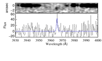
Figure 1: Zoom-in of the Q 0124+0044 X-shooter spectrum, centered on the Ly$\alpha$ line at $z=2.2616$. The top panel shows the 2D spectrum, smoothed by a Gaussian filter with a FWHM of 3 pixels, and centered on the quasar trace. Ly$\alpha$ emission from the DLA counterpart can be seen at an impact parameter of $\sim$1.3 arcsec below the quasar. The bottom panel shows the 1D spectrum extracted at the position of the offset Ly$\alpha$ emission, employing a flux scale in units of $10^{-19}$ erg s^-1 cm^-2 Å^-1. A Gaussian profile was fitted to the emission line, and is overlayed on the 1D spectrum (in blue).

2.3.2 Q 0139–0824

The absorber towards Q 0139–0824 was presented in Wolfe et al. (2008). A tentative detection of Ly$\alpha$ emission associated with the absorber at $z_{\rm abs}=2.6773$ was originally found with a low signal in IFU data from VLT/VIMOS (Programme ID 077.A-0450, PI: Christensen) but never published. To confirm the detection we conducted deeper follow-up spectroscopic observations using the VLT FORS spectrograph (Programme ID 081.A-0506, PI: Christensen). The deeper data confirmed the detection of Ly$\alpha$, spatially offset by $\sim$1.6 arcsec south-west of the quasar (see Fig. 2),and is published here for the first time. During subsequent X-shooter observations aimed at identifying additional emission lines (Programme ID 088.A-0378, PI: Christensen) a position angle of $-98\degr$ east of north was used. No additional emission lines at the DLA redshift were detected. However, given the redshift of the DLA, the strongest rest-frame optical emission lines are severely affected by telluric absorption. We note that the slit position angles used for spectroscopy do not correspond exactly to the position angle of the galaxy measured directly in the HST images, since sufficient spatial information about the counterpart was not available prior to the X-Shooter observations.

Integrating the Ly$\alpha$ line profile observed in the X-shooter spectrum gives a line flux of $f({\rm Ly}\alpha)=(2.2\pm 0.2)\times 10^{-17}$ erg s^-1 cm^-2 after correcting for Galactic extinction, and yields a lower limit to the SFR of $>0.7$ M_⊙ yr^-1.

In terms of origin and precision, the metallicity of the DLA towards Q 0139–0824 reported in the literature was rather uncertain. We therefore performed a new analysis of the absorption system using the X-shooter data. The new metallicity measurement is reported in Table 2 and the details of the absorption analysis are presented in Appendix A.

Extinction corrections are applied as follows for the F606W, F105W and F160W filters: 0.068, 0.022 and 0.014 mag, respectively.

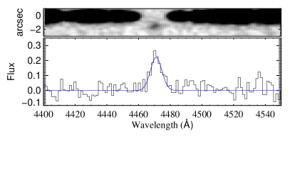
Figure 2: Zoom-in of the Q 0139–0824 FORS1 spectrum, centered on the Ly$\alpha$ line at $z=2.6773$. The top panel shows the 2D spectrum, smoothed by a Gaussian filter with a FWHM of 2 pixels, and centered on the quasar trace. Ly$\alpha$ emission from the DLA counterpart can be seen at an impact parameter of $\sim$1.6 arcsec below the quasar. The bottom panel shows the 1D spectrum extracted at the position of the offset Ly$\alpha$ emission, employing a flux scale in units of $10^{-17}$ erg s^-1 cm^-2 Å^-1. A Gaussian profile was fitted to the emission line, and is overlayed on the 1D spectrum (in blue).

2.3.3 Q 0310+0055

The emission counterpart of the absorber towards Q 0310+0055 was detected using long-slit spectra from Subaru/FOCAS (Kashikawa et al., 2014).

To accommodate the Subaru/FOCAS narrow-band detection ($\mathrm{mag}_{\mathrm{NB502}}=25.46\pm 0.13$; Kashikawa et al. 2014) in our stellar mass analysis (see Sect. 3.3), we first remove the contribution from Ly$\alpha$ line emission. Based on the reported Ly$\alpha$ luminosity of $L_{\mathrm{Ly}\alpha}=(1.07\pm 0.14)\times 10^{42}~{}\mathrm{erg~{}s}^{-1}$, and assuming a flat continuum shape over the NB502 bandpass, with a filter width of 60 Å, we obtain a NB continuum magnitude of $\mathrm{NB502}_{\mathrm{cont.}}=26.8\pm 0.6$. For the SED fits using LePhare (see Sect. 3.3), we construct a simple tophat narrow-band filter transmission curve with a central wavelength $\lambda_{c}=5025$ Å and a width of 60 Å. We also include their $B$- and $V$-band non-detections (25.32 and 25.50 magnitudes, respectively) reported as $3\sigma$ limits in 2 arcsec apertures at the position of the narrow-band detection. The observed Ly$\alpha$ line luminosity by Kashikawa et al. (2014) corresponds to a lower limit to the SFR of $>0.54$ M_⊙ yr^-1.

All magnitudes (measurements and limits) were corrected for Galactic extinction using the following corrections for the $B$, NB502, $V$, F105W, and F160W filters: 0.414, 0.343, 0.305, 0.082, 0.052 mag, respectively.

2.3.4 Q 0338–0005

The emission counterpart of the DLA towards Q 0338–0005 was originally detected by Krogager et al. (2012) as part of the VLT/X-shooter campaign, and was confirmed in an archival VLT/UVES spectrum by Bashir et al. (2019). Krogager et al. (2012) report the detection of Ly$\alpha$ emission at an impact parameter of 0.5 arcsec with a position angle of $-58\degr$ east of north. Krogager et al. (2017) report a lower limit to the SFR of $>0.3$ M_⊙ yr^-1 based on the line flux of Ly$\alpha$ as measured in the long-slit spectra taken during the X-shooter campaign.

The Galactic extinction is rather high for this sightline, with an extinction correction in the F606W filter of 0.207 mag.

2.3.5 Q 0918 +1636

There are two DLAs towards Q 0918+1636. The detection of the emission counterpart of the $z_{\rm abs}=2.583$ DLA was reported by Fynbo et al. (2011) and Fynbo et al. (2013) as part of the VLT/X-Shooter campaign. The authors detect emission lines from [O ii], [O iii], H$\alpha$ and H$\beta$ associated with the DLA at $z_{\rm abs}=2.583$ and infer a star formation rate of 8 M_⊙ yr^-1 based on the observed H$\alpha$ line flux.

Using HST data, Fynbo et al. (2013) detect the continuum emission of the DLA at $z_{\mathrm{abs}}=2.583$ at an impact parameter of 1.98 arcsec from the quasar at a position angle of $-115\degr$ east of north, and obtain a stellar mass of $\log({\rm M}_{\star}/{\rm M_{\odot}})=10.1_{-0.1}^{+0.2}$.

In addition to the re-reduced HST images and their associated magnitudes, we also include the Galactic extinction corrected SDSS $u$, $g$, and K_s-band observations from the Nordic Optical Telescope NOTCam (Abbott et al., 2000) reported by Fynbo et al. (2013). For the F606W, F105W and F160W magnitudes we adopt extinction corrections of 0.058, 0.018 and 0.012 mag, respectively.

Fynbo et al. (2013) furthermore detect emission lines from Ly$\alpha$ and [O iii] $\lambda$5007 associated with the second absorber at $z_{\rm abs}=2.412$ at a very small impact parameter $<0.25$ arcsec at a position angle of $\sim 130$ deg east of north. We are not able to test for such an object in our HST imaging data, as detailed in Sect. 3.1, due to the strong residuals of the quasar PSF subtraction at these small impact parameters.

2.3.6 Q 1313+1441

The emission counterpart of the absorber towards Q 1313+1441 was detected by Krogager et al. (2017) as part of the X-shooter campaign (Fynbo et al., 2010; Krogager et al., 2017). The detection is based on Ly$\alpha$ emission in the trough of the damped Ly$\alpha$ absorption profile at an impact parameter of 1.3 arcsec. The authors report detections in two slits with different orientations yielding seemingly inconsistent relative positions of the emission. The quoted impact parameter refers to the brighter of the two detections.

Krogager et al. (2017) suggest that the two detections may arise from two different neighbouring galaxies. With the HST data in hand, we can revise this explanation. We do not detect multiple counterparts around the quasar that would coincide with the detections reported by Krogager et al. (2017). Instead, we identify a single counterpart in the near-infrared data with an extended, disturbed structure (see Sect. 3.1). Such an extended structure could explain the appearance of emission in the two slits at orientations of +60 and $-$60$\degr$ (east of north) used by the authors.

Extinction corrections for the F606W, F105W and F160W filters are applied as follows: 0.051, 0.016 and 0.010 mag, respectively.

2.3.7 Q 2059–0528

The emission counterpart of the DLA towards Q 2059–0528 was detected by Hartoog et al. (2015), as part of the X-Shooter campaign (Fynbo et al., 2010; Krogager et al., 2017). The authors tentatively detect Ly$\alpha$ emission in all three slit orientations (at $\sim 3\sigma$ in individual slits). By stacking all three observations, Hartoog et al. (2015) obtain a robust detection in Ly$\alpha$ of $f_{\rm Ly\alpha}=(10.19\pm 1.67)\times 10^{-18}$ erg s^-1 cm^-2. The Ly$\alpha$ line flux provides a lower limit to the SFR of $>0.2$ M_⊙ yr^-1. The fact that emission is seen in all three slits suggests a low impact parameter for the counterpart ($<$0.75 arcsec).

Péroux et al. (2012) used VLT/SINFONI IFU observations to search for H$\alpha$ emission associated to the absorber. They report a non-detection, which translates into an upper limit to the SFR of $<1.4$ M_⊙ yr^-1.

Extinction corrections for the F606W, F105W and F160W filters are applied as follows: 0.104, 0.033 and 0.021 mag, respectively.

2.3.8 Q 2222 –0946

The counterpart of the absorber towards Q 2222–0946 was detected by Fynbo et al. (2010) as part of the VLT/X-shooter campaign. The authors report a detection of the emission counterpart at an impact parameter of 0.8 arcsec, at a predicted position angle of $\sim 40\degr$ based on triangulation from the observations with different slit orientations. Using HST data, Krogager et al. (2013) confirm the detection at an impact parameter of 0.74 arcsec.

Using deep VLT/X-shooter data obtained with the slit aligned towards the emission counterpart, Krogager et al. (2013) detect emission from Ly$\alpha$, [O ii], [O iii], H$\alpha$, and H$\beta$ lines. Further data was obtained from Keck/Osiris (Jorgenson & Wolfe, 2014) and VLT/SINFONI (Péroux et al., 2012). Krogager et al. (2013) report a SFR based on H$\alpha$ of 13 M_⊙ yr^-1 and a stellar mass of $\log({\rm M}_{\star}/{\rm M_{\odot}})=9.3\pm 0.2$ based on SED fitting.

For the F606W, F105W and F160W magnitudes we adopt extinction correction factors of 0.103, 0.032 and 0.021 magnitudes, respectively.

2.3.9 Q 2239–2949

The emission counterpart of the absorber towards Q 2239–2949 was identified by Zafar et al. (2017). The authors report a detection of Ly$\alpha$ emission at $z_{\rm abs}=1.825$ spatially offset by 2.4 arcsec from the quasar. The Ly$\alpha$ emission line flux of the counterpart translates into a lower limit on the SFR of $>0.07\pm 0.01$ M_⊙ yr^-1. The absorber is a sub-DLA and no ionisation correction was applied to the reported metallicity, which should therefore be interpreted with care.

We adopt the following extinction corrections for the F606W, F105W and F160W filters: 0.043, 0.013, and 0.009 mag, respectively.

2.3.10 Q 2247–6015 (alternative name: HE 2243–60)

The absorber towards Q 2247–6015 was first analysed by Lopez et al. (2002) using data from VLT/UVES. Bouché et al. (2012, 2013) conducted comprehensive followup observations of the quasar field using VLT/SINFONI IFU data and detect the associated counterpart in H$\alpha$ at an impact parameter of 3.1 arcsec. The authors report a dust-corrected H$\alpha$ star formation rate of 33 M_⊙ yr^-1, which owing to the aperture-free IFU data is not affected by slit-losses.

Extinction corrections for the F606W, F105W and F160W filters are applied as follows: 0.047, 0.015 and 0.009 mag, respectively.

3 Results

Based on the HST observations presented in Sect. 2.2, we successfully detect continuum emission for all targets in our sample in at least one filter (nine robust detections; one tentative detection in the Q 0338–0005 field, see Fig. 3 and Fig. 4). Eight of these continuum detections are presented in this work for the first time (the seven targets associated with Programme ID 14122 and the previously unpublished Q 0338–0005 observation associated with Programme ID 12553). We analyse the surface brightness distributions of the detected continuum emission and provide measurements of the half-light radii (see Sect. 3.2).

For eight of the ten targets in our statistical sample (six associated with Programme ID 14122 and the two re-analysed objects associated with Programme ID 12553), we secure detections in more than one filter, which enables us to estimate the SFR and stellar mass by modelling the photometric spectral energy distributions (see Sect. 3.3). Our analysis of the HST data is presented below.

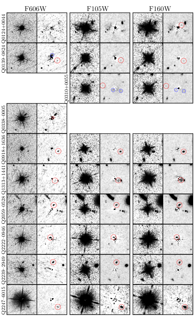
Figure 3: Mosaic of 9$\times$9 arcsec cutouts centered on each quasar. Rows show individual targets. Each column of two sub-panels shows one HST filter. Each sub-panel displays the science image (left) and quasar subtracted residual image (right) with confirmed detections (red circles) and proximate candidates with no redshift information (blue circles). Each panel is aligned north up, east left. Science images are displayed with a histogram equalisation to enhance faint structures, and residual images are Gaussian smoothed with a fixed smoothing-length of 0.06 arcsec.

3.1 Subtraction of quasar point spread function

To detect the faint stellar continuum of the absorbing galaxy and to search for objects hiding under the bright quasar PSF, we must isolate the flux from the quasar and subtract it from each image. Traditionally for HST images, a synthetic PSF is either created using TINYTIM, or empirically modelled from bright, unsaturated stars in the same exposure (e.g. Kulkarni et al., 2000; Krogager et al., 2013; Fynbo et al., 2013). The former method is noiseless, can be constructed for the position of the quasar on the detector, and captures the profile of the outer PSF wings. However, the model is limited by the details in its construction; by the accuracy of the recorded telescope aberrations; and can produce unsatisfactory models for saturated objects (e.g. Krogager et al., 2013). The latter, empirical method takes advantage of the high S/N of bright stars and is observed simultaneously with the quasar, which mitigates temporal differences. However, this method is sensitive to the position of the bright star on the detector plane and aberrations of the telescope. The empirical approach is often unable to model the extended wings of the PSF as the outer regions are dominated by noise in the sky background. Further limitations include the number of suitable stars in the field as well as potential colour differences between the object of interest (in our case, the quasar) and the stars used to construct the PSF model (Warren et al., 2001).

Since our HST programme targets multiple quasar fields with the same observing strategy, and since the final data products are combined with identical settings (see Sect. 2.2), the aforementioned caveats can be mitigated by modelling the quasar PSF (qPSF) from the targeted quasars themselves (e.g. Warren et al., 2001; Augustin et al., 2018). For each quasar ($i=1...10$) in a given band, we construct empirical, non-parametric models of qPSF_i from the median-combined stack of all remaining qPSFs of the same filter. Before combining the images, the individual images are sub-sampled on a 4-times finer grid and re-centered to the PSF centroid.

Finally, our empirically constructed qPSF models are resampled back to the original binning and fitted to their respective quasar image in order to subtract the quasar emission, see Fig. 3. After subtracting the qPSF, we search the field for faint stellar continuum emission associated with the foreground absorber at the locations identified in previous spectroscopic observations (highlighted as red circles in Fig. 3). Moreover, we can look for potential candidates at smaller impact parameters down to a limit of $\sim 0.5$ arcsec where residuals from the qPSF subtraction start to dominate (blue circles in Fig. 3).

In the field of Q 0139–0824, we identify a bright object in the F606W band at low impact parameter (blue circle in Fig. 3). This object clearly overlaps with the quasar PSF, but is unidentified in the other bands. We therefore revisited the quasar spectrum to see whether this object has an absorber counterpart. The spectrum reveals a weak absorber at a redshift $z_{\rm abs}=2.233$, which we hypothesise is the counterpart of the bright object. However, the absorption lines are too weak to be compatible with a strong H i absorber, and we therefore leave it to be pursued in future work. Alternatively, the object may be part of the quasar’s local galactic environment.

For Q 0310+0055, we note that our PSF subtracted images reveal two objects at lower impact parameters (blue circles in Fig. 3). However, Kashikawa et al. (2014) do not detect ${\rm Ly}\alpha$ emission at the absorber redshift at lower impact parameters. Since evidence for a physical connection is absent, we disregard them in the remainder of this work, but note that the detections may be either nearby galaxies that do not emit ${\rm Ly}\alpha$; part of the local environment of the quasar; or simply low-redshift interlopers. Further spectroscopic investigation of the field is needed to reveal the nature of these objects.

In the field of Q 0338–0005, we only obtain a tentative detection of the counterpart observed in spectroscopy by Krogager et al. (2012). The tentative detection of the continuum emission of the counterpart is shown in Fig. 4, located at an impact parameter of $0.39\pm 0.02$ arcsec from the quasar line of sight at a position angle of $-55\pm 2\degr$. The impact parameter and position angle are consistent with those reported by Krogager et al. (2017). Nonetheless, given the strong residuals of the PSF subtraction we only consider this a tentative detection.

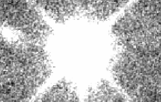
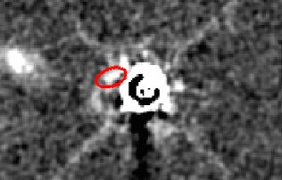
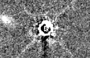
Figure 4: Tentative detection of the counterpart associated with the DLA towards Q 0338–0005. The panels show from top to bottom: a zoom-in of the quasar; the image after subtraction of the qPSF; and the residuals after simultaneously fitting the qPSF and the tentative counterpart. The location of the tentative counterpart is shown by the red ellipse in the middle panel. Note that the panels display the native image axes.

For Q 2059–0528, the PSF-subtracted image reveals multiple objects, all of which have larger impact parameters than the limit ($b<0.75$ kpc) reported by Hartoog et al. (2015). We note, however, that this limit is based on the assumption that the individual Ly$\alpha$ signals in the three slits are detecting the same counterpart. Relaxing this assumption, we note that their reported detection in the $\mathrm{PA}=-60\degr$ slit is the only detection formally above $3\sigma$ significance. We therefore identify the bright object immediately north-west of the quasar as the most likely source of the Ly$\alpha$ emission, and as a candidate counterpart to the DLA. The impact parameter of 1.43 arcsec measured in our HST image is furthermore consistent with the location of the emission in the spectrum with slit angle $\mathrm{PA}=-60\degr$ by Hartoog et al. (2015). Such a configuration with several components seen in emission appears similar to the DLA host galaxy system towards Q 2206–1958, shown to be in an active stage of merging (Møller et al., 2002; Weatherley et al., 2005).

3.2 Modelling surface brightness profiles

Having identified the continuum emission counterparts, we use galfit (Peng et al., 2002) to model their surface brightness profiles. Here, we do so by iteratively adding Sérsic components that are fitted simultaneously with the quasar point source until the galaxy emission is fully captured. We set up galfit to resample the PSF back to its original binning during fitting. galfit automatically takes the PSF convolution into account when performing the fit.

galfit has been used to derive structural parameters and magnitudes for individual absorption-selected galaxies in the past (e.g. Krogager et al., 2013; Fynbo et al., 2013; Augustin et al., 2018). We here make an effort to outline and emphasise certain aspects of the fitting procedure in this work that differ from the standard case of retrieving parameters for a galaxy on a flat sky background.

• The brightness of the quasar causes the qPSF profile to extend far into the field. It is therefore essential to use a large PSF model, capable of subtracting the flux in the PSF wings. If the PSF does not account for this, galfit will overestimate the sky background.

• The large PSF model necessitates a large fitting region. We found that a fitting region of 800$\times$800 pixels for a pixel scale of 0.067 arcsec per pixel was needed to ensure robust quasar magnitudes matching known SDSS optical photometry.

• The Sérsic function associates higher light concentrations with larger extended wings. Any over/under estimation of either the sky background and/or the quasar PSF wing will therefore be compensated for by (wrongfully) adjusting the Sérsic index. This will minimise the $\chi^{2}$ statistic at the expense of unrealistically large concentrations. It is therefore essential to fit the galaxy and quasar simultaneously, and determine the background independently. This is particularly important as our objects lie at small impact parameters. Given the high contrast between the quasar and the galaxy brightness, a small change in the quasar magnitude may generate large differences in final galaxy parameter estimates.

We therefore fix the sky value to independent measurements determined from the mean of the pixel counts in sky regions free of sources and hot pixels. The zero-point (ZP) for each filter was calculated with the PHOTPLAM and the PHOTFLAM FITS header keywords, giving values of ZP${}_{\rm F606W}=26.104$; ZP${}_{\rm F105W}=26.270$; and ZP${}_{\rm F160W}=25.947$. Finally, we pass the science image to galfit in the recommended units of counts. This is particularly relevant for our science case, as the brightness contrast between the quasar and the galaxy causes pixel values to span a large dynamic range.

Adopting a single Sérsic component does not capture the clumpy light distribution observed in many of the objects, but results in large residuals. This behaviour is also reflected in the galfit solution, which under such conditions (or for faint objects) becomes unstable to perturbations in initial parameter values. Iteratively adding Sérsic components, which collectively capture the effective light distribution of the source, stabilises the parameter range within physically acceptable Sérsic indices $(0.5\leq n\leq 8)$ and effective semi-major axes ($0.2\leq a_{e}~{}/~{}\mathrm{pixels}\leq 20$), although the distribution of the parameters remains sensitive to the initial guesses, giving near-identical $\chi^{2}$-statistics for different combinations.

For Q 1313+1441, the fit to the extended and disturbed structure identified as the emission counterpart requires the introduction of an intermediate Sérsic profile to converge on a satisfactory model. The galfit solution suggests a bright component $\sim 0.7$ arcsec from the quasar, but at this proximity it is sensitive to quasar subtraction residuals, and it lies a factor of two off the triangulated position (see Sect. 2.3.6). We therefore choose to disregard this component when reporting the results, and emphasise that further work is needed to establish the nature of the bright signal detected in both the IR bands.

The final fits suggest that $\sim 40\%$ of absorption-selected galaxies at redshift $z\sim 2-3$ require multiple Sérsic profiles to mitigate apparent systematic residuals and accurately capture the light distribution (for individual number of Sérsic components employed in each fit, see Table 3). We note that the number of Sérsic profiles employed for each host galaxy should be considered lower limits, as they correlate with spatial resolution. However, the fact that $40\%$ reveal multiple star-forming clumps at a drizzled F160W spatial resolution of 0.067 arcsec per pixel at $z\sim 2-3$ agrees with the general trend of clumpy morphologies of high-redshift galaxies (Livermore et al., 2015).

3.2.1 Non-parametric size measurements

Previous studies, often motivated by observational considerations, chose to report structural parameters and morphology based on the band with the highest spatial resolution. Here, we attempt a physically motivated approach, and report morphologies based on the reddest (F160W) band in order to capture the main stellar component. We then fix the morphology in the remaining bands to that derived in F160W, appropriately scaled and rotated to the resolution, pixel sampling and orientation of individual frames.

To systematically analyse and compare objects fitted with a single Sérsic profile to those that require multiple components we adopt a conservative approach, and report non-parametric half-light radii ($r_{1/2}$) calculated from growth curves originating at the centroid of each galaxy model together with its total magnitudes (summed over individual Sérsic components). For $r_{1/2}$ the final uncertainty reflects an inverse variance weighted sum of the relative uncertainties from each component contributing to the model. We estimate magnitude errors from the flux of the modelled light distribution and flux errors measured directly in the quasar and galaxy subtracted residual image as $\Delta F=\sqrt{\sum_{i\in A}\sigma^{2}_{\mathrm{tot},i}}$, where $A$ is the non-masked pixels in a $5\times r_{1/2}$ circular aperture at the position of the centroid of the galaxy model, and $\sigma_{\mathrm{tot},i}$ is the residual flux in pixel $i$. These results are recorded in Table 3.

3.2.2 Comparison to literature measurements

Independent galfit-based sizes were reported for the sources in the fields of Q 2222–0946 (Krogager et al., 2013; Augustin et al., 2018, both based on the F606W filter) and Q 0918+1636 (Fynbo et al., 2013, based on the F160W filter). In the former field, Krogager et al. (2013) report an effective semi-major axis of $a_{e}=1.12\pm 0.06$ kpc, and Augustin et al. (2018) find a corresponding value of $a_{e}=1.5\pm 0.1$ kpc. To compare these size measurements with our growth curve based $r_{1/2}$, we convert the reported $a_{e}$ to circularised radii as $r_{\text{circ}}=a_{e}\times\sqrt{b/a}$, where $b/a$ refers to the semi-major-to-minor axis-ratio. For $b/a=0.17\pm 0.02$ (Krogager et al., 2013) we obtain $r_{\text{circ}}=0.46\pm 0.03$ kpc (consistent with our $r_{1/2}$ measurement within $1.4\sigma$). Augustin et al. (2018) report an axis ratio of $b/a=0.38\pm 0.06$, which translates to $r_{\text{circ}}=0.9\pm 0.1$ kpc (indicating a $\sim 3.6\sigma$ tension with our value).

For the counterpart of the $z=2.583$ DLA towards Q 0918+1636, Fynbo et al. (2013) report values of $a_{e}=1.4\pm 0.1$ kpc and $b/a=0.4\pm 0.1$ which translates into $r_{\text{circ}}=0.9\pm 0.2~{}\mathrm{kpc}$, perfectly consistent with our $r_{1/2}$ measurement. These results demonstrate that our generalised method to retrieve non-parametric half-light radii is robust and provides consistent results with those from the literature. The $\sim 3.6\sigma$ tension between our $r_{1/2}$ and the circularised effective radius reported by Augustin et al. (2018) cannot purely be attributed to the analysis being performed in different filters (theirs using F606W; ours using F160W) and therefore sampling different underlying stellar populations. Our size measurement is consistent with the value obtained by Krogager et al. (2013), based on their analysis of the F606W filter image. Nor can the discrepancy be explained by methodological differences, as our $r_{1/2}$ measurements agree remarkably well with the $r_{\text{circ}}$ of two separate studies, conducted in two independent quasar fields (Fynbo et al., 2013; Krogager et al., 2013).

Table 3: Results of galfit modelling of absorber counterparts.

Target	NS	P.A.	$\theta$	$b$	$r_{1/2}$	magF606W	magF105W	magF160W
		[deg]	[arcsec]	[kpc]	[kpc]	[AB]	[AB]	[AB]
Q0124$+$0044	$1$	$311\pm 1$	$1.25\pm 0.04$	$10.5\pm 0.3$	$0.4\pm 3.1$	–	–	$26.9\pm 0.2$
Q0139$-$0824	$1$	$244.6\pm 0.7$	$1.83\pm 0.03$	$14.8\pm 0.2$	$0.4\pm 1.5$	$27.2\pm 0.1$	$27.3\pm 0.2$	$26.8\pm 0.1$
Q0310$+$0055	$1$	$77.9\pm 0.5$	$3.77\pm 0.04$	$29.4\pm 0.3$	$0.5\pm 0.9$	–	$26.9\pm 0.1$	$26.7\pm 0.1$
Q0338$-$0005	$1$	$305\pm 2$	$0.39\pm 0.02$	$3.3\pm 0.2$	$1.5\pm 0.1^{a}$	$25.7\pm 0.1^{a}$	–	–
Q0918$+$1636	$1$	$245.78\pm 0.06$	$2.00\pm 0.01$	$16.37\pm 0.02$	$0.81\pm 0.03$	$25.65\pm 0.06$	$24.53\pm 0.03$	$23.66\pm 0.01$
Q1313$+$1441	$2$	$241\pm 2$	$1.20\pm 0.04$	$10.3\pm 0.4$	$2.2\pm 0.7$	$26.7\pm 0.4$	$26.5\pm 0.3$	$25.7\pm 0.2$
Q2059$-$0528	2	$334.8\pm 0.3$	$1.43\pm 0.01$	$12.05\pm 0.09$	$1.7\pm 0.3$	$25.23\pm 0.08$	$24.71\pm 0.08$	$23.74\pm 0.06$
Q2222$-$0946	$1$	$41.1\pm 0.2$	$0.74\pm 0.01$	$6.17\pm 0.02$	$0.52\pm 0.03$	$24.32\pm 0.03$	$24.59\pm 0.09$	$23.63\pm 0.06$
Q2239$-$2949	3	$348.8\pm 0.7$	$2.31\pm 0.03$	$19.8\pm 0.3$	$1.5\pm 0.4$	$25.00\pm 0.06$	$24.39\pm 0.03$	$24.05\pm 0.03$
Q2247$-$6015	$2$	$222.3\pm 0.3$	$2.99\pm 0.02$	$25.0\pm 0.2$	$2.6\pm 0.3$	$23.48\pm 0.06$	$23.33\pm 0.07$	$22.65\pm 0.04$

N_S refers to the number of Sérsic components used in the fit. The position angle (P.A.) of the galaxy position relative to that of the quasar is measured in degrees east of north. Magnitudes are tabulated without correction for Galactic extinction.

^a The fit of the tentative counterpart of Q0338–0005 required highly fine-tuned parameters. The half-light radius and the associated magnitude should therefore be treated with caution.

Table 4: Results of SED modelling of absorber counterparts.

Target	$E_{B-V}$	$\log(\text{SFR}/\mathrm{M}_{\odot}~{}\mathrm{yr}^{-1})$	$\log(\mathrm{M}_{\star}/\mathrm{M}_{\odot})$
Q0124$+$0044	–	–	–
Q0139$-$0824	0.00	$0.0\pm 0.3$	$8.2\pm 0.2$
Q0310$+$0055	0.00	$0.4\pm 0.3$	$8.6\pm 0.3$
Q0338$-$0005	–	–	–
Q0918$+$1636	0.25	$1.3\,^{+0.1}_{-0.2}$	$10.2\,^{+0.1}_{-0.2}$
Q1313$+$1441	0.00	$0.0\pm 0.3$	$8.6\,^{+0.4}_{-0.6}$
Q2059$-$0528	0.20	$1.2\,^{+0.3}_{-0.4}$	$9.7\,^{+0.6}_{-0.5}$
Q2222$-$0946	0.00	$0.9\,^{+0.2}_{-0.1}$	$9.2\pm 0.1$
Q2239$-$2949	0.35	$1.7\pm 0.2$	$9.0\pm 0.1$
Q2247$-$6015	0.10	$1.6\pm 0.3$	$9.8\,^{+0.7}_{-0.6}$

Star formation rates and stellar masses are reported as median values with $1\sigma$ uncertainties based on the 16th- and 84th percentiles, determined using the built-in maximum likelihood routine of LePhare.

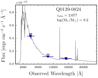
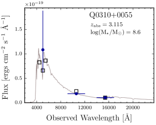
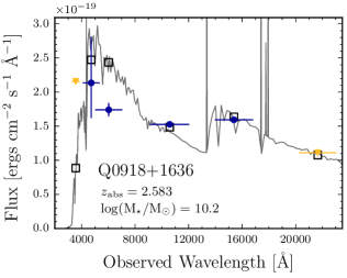
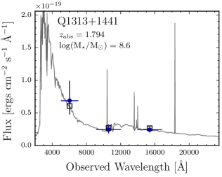
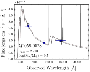
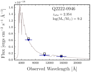
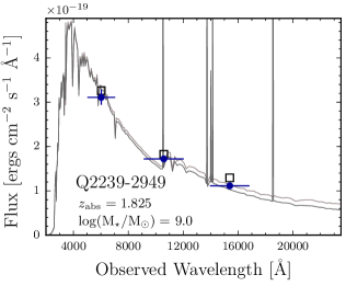
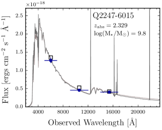
Figure 5: Spectral energy distribution (SED) for the objects where a fit was possible. Blue (yellow) filled symbols refer to included measurements (limits), with horizontal error-bars indicating the FWHM of each filter. Grey empty squares show the best-fit transmission-weighted filter-flux. The two SEDs in each panel show the best fit with and without nebular emission. In many cases the two fits overlap, indicating the robustness of the solution. Each panel displays target name, absorber redshift, and the SED-based stellar mass of the counterpart. The conservative B- and V-band non-detections reported in Kashikawa et al. (2014) were included as upper limits during fitting, but lie above the Q0310$+$0055 panel’s displayed flux range.

3.3 Modelling the spectral energy distribution

We determine the stellar mass (M_⋆) for each of the absorbing galaxies by fitting the SEDs using the code LePhare (Arnouts et al., 1999; Ilbert et al., 2006). For each target, we fix the redshift and apply the corrections for Galactic extinction to the magnitudes. LePhare fits the SEDs by minimising $\chi^{2}$ across a user defined grid of parameters. As input, we use standard Bruzual & Charlot (2003, BC03) single stellar population (SSP) templates for a Chabrier (2003) IMF, with default model metallicities $Z/Z_{\odot}=$ 0.2, 0.4 and 1.0. We assume exponentially declining star formation histories with $e$-folding time-scales spanning 0.1 – 30 Gyrs and limit the stellar population ages to span $0-4~{}\mathrm{Gyrs}$, which corresponds to the age of the Universe at the lowest absorption-redshift in our sample. We adopt a Calzetti et al. (2000) attenuation-curve as we are probing redshifts around the peak of cosmic star formation. The colour excess, $E_{B-V}$, is sampled in steps of 0.05 in the range $0-0.3$ mag. The range is extended, as needed, to ensure that the preferred $E_{B-V}$ is associated with a $\chi^{2}$-minimum rather than a grid-boundary.

The resulting SED fits of the absorbing galaxies are shown in Fig. 5 and the resulting colour excesses, SFRs and stellar masses are reported in Table 4.

All values are based on SED fits including the nebular emission lines apart from Q 2222–0946 and Q 0310+0055, for which information on spectroscopic emission-line fluxes was used to isolate the stellar continuum (see Krogager et al., 2013; Kashikawa et al., 2014, respectively). For completeness, we also overplot the best-fit SEDs using the same grid, but excluding emission lines.

3.3.1 Comparison to literature measurements

In the case of Q 2222–0946, we correct our F160W broadband magnitude for a 33% nebular emission-line contribution, as determined by Krogager et al. (2013). This yields results which are in good agreement with those presented by Krogager et al. (2013), despite their use of a randomised library of different star formation histories instead of a parameterised approach as we have assumed in this work. The consistency between these results is contrasted by the measurement of $\log(\mathrm{M}_{\star}/\mathrm{M}_{\odot})=9.7\pm 0.3$ reported by Augustin et al. (2018). Similar to our work, the authors use LePhare for their analysis; However, our parameter-grids differ in important aspects. In particular, their models use a single burst of star formation whereas we allow for a range of star formation histories. It is also unclear (i) how they include dust reddening (both in range and sampling); (ii) whether they correct their magnitude measurements, adopted from Krogager et al. (2013), for Galactic extinction; and (iii) whether the template fit included nebular emission (as supported by the SED fits presented in Figure 5 by Augustin et al. (2018)), or not (as supported by Table 3 of Augustin et al. (2018) in which they report the F160W nebular-emission corrected continuum magnitude of Krogager et al. (2013)). Indeed, by restricting the input models to a single burst population, using the F160W magnitude which includes the emission-line flux reported by Krogager et al. (2013), and enabling LePhare’s nebular emission prescription, we are able to retrieve a stellar mass of $\log(\mathrm{M}_{\star}/\mathrm{M}_{\odot})=9.6\pm 0.3$ which is in closer agreement with the value reported by Augustin et al. (2018), whilst maintaining a near identical star formation rate of $\log(\text{SFR}/\mathrm{M}_{\odot}~{}\mathrm{yr}^{-1})=0.9\pm 0.2$ to that which we report based on our own grid (see Table 4).

Our magnitude measurements reported for Q 0918+1636 (see Table 3) appear in tension with those reported by Fynbo et al. (2013, their table 2). Whereas our values refer to the measured observables, Fynbo et al. (2013) tabulated the magnitudes after applying Galactic extinction corrections. Once these corrections are applied to our measurements (Sect. 2.3), all magnitudes are consistent within $\lesssim 1\sigma$. Reassuringly, the stellar mass of the DLA counterpart derived in this work is in perfect agreement with the value of $\log(\mathrm{M}_{\star}/\mathrm{M}_{\odot})=10.1^{+0.2}_{-0.1}$ reported by Fynbo et al. (2013, their Table 3).

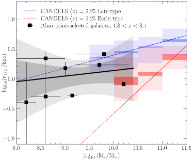
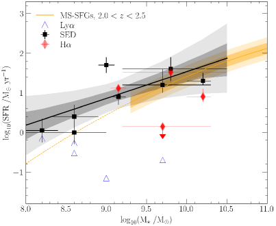
Figure 6: The mass–size relation (left) and the ‘main sequence’ of star-forming galaxies (right) of our sample of absorption-selected galaxies at $z\sim 2.3$ observed with HST. The absorption-selected galaxies preferentially select the star-forming galaxy population, with an extension to lower stellar masses. In both panels, the black line and its associated grey shaded regions depict the best fit relation and the $1\sigma-$ and $2\sigma$ confidence intervals to the absorption-selected galaxies presented in this work. The fit in the right panel uses only the SED-based SFRs (black squares). In the left panel, we show the scaling relations observed for luminosity-selected samples of early-type (red) and late-type (blue) galaxies at redshifts $\langle z\rangle=2.25$ by van der Wel et al. (2014), with dark shaded regions representing medians and their errors and the light shaded regions representing the 16- and 84-percentile ranges. Solid lines show the relations derived from effective semi-major axis measurements, with dashed segments illustrating an extrapolation beyond the reported completeness limits. The box-shaped shaded regions show the mean and $1\sigma$ scatter of circularised radii, whose definition is closer to our half-light radii. In the right panel, we show the ‘main sequence’ of star-forming galaxies at redshifts $2.0<z<2.5$ (MS-SFGs, yellow line) from Whitaker et al. (2014), with yellow shaded regions indicating the $1\sigma$ and $2\sigma$ confidence intervals including the scatter in the data from Whitaker et al. (2015). The extrapolation to lower masses is illustrated by the dashed segments. The black squares show SFR measurements based on the SED fit whereas red diamonds show spectroscopic measurements based on H$\alpha$. The blue triangles represent SFR lower limits based on ${\rm Ly}\alpha$.

4 Discussion

Having analysed the emission properties of our sample of high-redshift galaxies associated with strong H i absorbers, we can now investigate how these objects compare to samples of luminosity-selected galaxies. In Fig. 6 we show the established mass–size relation (van der Wel et al., 2014) and the so-called ‘main sequence’ of star-forming galaxies (MS-SFGs) from Whitaker et al. (2014), both constructed from luminosity-selected samples at similar redshifts to our sample, which has a mean redshift $\langle z_{\rm abs}\rangle=2.3$. A more detailed comparison of our HST sample to each of these relations is presented below.

4.1 Mass–size relation

van der Wel et al. (2014) investigate the stellar-mass–size relation for early- and late-type galaxies over a large range in redshift based on the 3D-HST/CANDELS survey. Early- and late-type galaxies are separated by colour-criteria. The authors derive stellar masses assuming the same initial mass function (Chabrier, 2003) as we do in this work. van der Wel et al. report their size estimates in two ways; as the effective semi-major axis ($a_{e}$) from Sérsic models; and as circularised effective radii. In Fig. 6, we indicate the mass–$a_{e}$ relations for early- and late-type galaxies at $\langle z\rangle=2.25$ reported by van der Wel et al. (2014) as the red and blue lines, respectively. Below the reported completeness limits of their work, we show an extrapolation of these relations as dashed lines. The circularised effective radii by van der Wel et al. are shown as shaded boxes, where the vertical extent depicts the $1\sigma$ dispersion within a given stellar mass bin, and the horizontal extent depicts the stellar mass range of the bin. We note that the circularised radii, in definition, more closely resemble our non-parametric approach, and should therefore make a more fair comparison to the $r_{1/2}$ size-estimates of the absorption-selected galaxy sample presented in this work.

In Fig. 6, we also show our sample of absorption-selected galaxies. We fit a mass–size relation to our sample with a power-law, similar to van der Wel et al. 2014. For the fit, we adopt the minimisation method described in Møller et al. (2013) including a term for the intrinsic scatter, and taking into account the asymmetric uncertainties in $\log({\rm M}_{\star}/\mathrm{M}_{\odot})$ and measured radii. We obtain the following best fit relation:

$$\log(r_{\mathrm{1/2}}/{\rm kpc})=(-0.8_{-2.0}^{+2.3})+(0.1\pm 0.2)\log({\rm M}_{\star}/{\rm M_{\odot}})~{},$$

with an internal scatter of $\sigma_{\log r_{1/2}}=0.26$ dex. The best-fit relation for our sample is shown as the solid black line with $1\sigma$- and $2\sigma$ confidence intervals shown as grey shaded regions around the line. The relation inferred from our sample matches more closely the relation for late-type (blue) galaxies than the one for early-type (red) galaxies. Quantitatively, we assess the similarity between our sample and the two relations for early- and late-type galaxies using the reduced $\chi^{2}$ statistic. For eight degrees of freedom ($\nu=8$) and assuming a simple extrapolation of the relations from luminosity-selected galaxies, we obtain $\chi^{2}/\nu=9.5/8=1.2$ to the blue line, and $\chi^{2}/\nu=70/8=8.8$ to the red line. Given the number of degrees of freedom, the expectation value of the reduced $\chi^{2}$ statistic is $\chi^{2}/\nu\approx 1\pm\sqrt{2/\nu}\approx 1.0\pm 0.5$. We therefore conclude that our sample is consistent (to within $<1\sigma$) with the relation for late-type galaxies and inconsistent with the relation for early-type galaxies at more than $15\sigma$.

Albeit limited by sample size and individual measurement uncertainties, it is encouraging to see that, even towards the low-mass end, our absorption-selected sample follows the extrapolated luminosity-selected mass-size relation for late-type galaxies at $z\sim 2$. This result is consistent with the notion that identifying galaxies in absorption preferentially selects faint, gas-rich, star-forming galaxies (e.g., Fynbo et al., 1999). Remarkably, more than $50\%$ of our sample has stellar masses below the formal completeness limit of the luminosity-selected HST survey, despite the fact that our metallicity cut pre-selects the most massive (sub-)DLA galaxies known.

4.2 Main sequence of star-forming galaxies

In this section we consider only the sub-sample of 8 galaxies for which we derive SED-based SFRs and stellar masses, as listed in Table 4.

In Fig. 6, we show the polynomial parameterization of the MS-SFGs for the luminosity-selected galaxies at $z\sim 2-2.5$ reported by Whitaker et al. (2014), with the associated $1\sigma-$ and $2\sigma$ scatter in the relation based on the intrinsic dispersion $\sigma_{\rm intrinsic}=0.14$ reported in Whitaker et al. (2015). For our sample, we have incomplete data from three different SFR tracers: lower limits from ${\rm Ly}\alpha$; recombination-line measurements of H$\alpha$ which trace the near-instantaneous SFR on time-scales of $\sim 10$ Myr; and SED-based values (see Section 3.3) that trace the ongoing SFR (see the documentation of LePhare). To form a complete census, we plot all the SFR tracers for each object in Figure 6.

The results of the various diagnostics can be summarised as follows. For objects with SFR measurements in ${\rm Ly}\alpha$ and either H$\alpha$ or SED, the lower limits from ${\rm Ly}\alpha$ are consistent with the other tracers in all cases. Considering the limited number of photometric bands available to constrain our SED fits, we find a good agreement between H$\alpha$ and SED based SFRs where both are available, with the notable exception of Q 2059–0528. For this object, expressed in terms of logarithmic SFR, our SED based measurement is in 2.6$\sigma$ tension with the H$\alpha$ upper limit reported by Péroux et al. (2012). We note, however, that the H$\alpha$ limit may be underestimated due to the added uncertainties introduced by the quasar PSF and its subtraction. In addition, the characteristic SFR timescales differ, and our HST filter selection is optimised for the determination of SED-based stellar masses, not of SED-based SFRs. We therefore resort to the SED-based SFR on a statistical level of the sample, but emphasise caution not to overinterpret the SED-based SFR for individual objects.

Since the SED-based SFRs are available for all galaxies in the sub-sample treated in this section, we use these SFR estimates to investigate the relation between stellar mass and star formation. A log-linear (i.e., power-law) fit of the stellar-mass–SFR_SED relation using an orthogonal linear regression method with asymmetric uncertainties to our sample yields:

$$\log({\rm SFR}/\textrm{M${}_{\odot}$~{}yr${}^{-1}$})=(0.7\pm 0.5)\log({\rm M_{\star}/M_{\odot}})-(5.2\pm 4.3)~{}.$$

In Fig. 6 we plot the best-fit relation to our sample as a solid black line, and its $1\sigma$ and $2\sigma$ confidence intervals as grey shaded regions around the line.

The MS-SFG relation at $2.0<z<2.5$ by Whitaker et al. (2014) suggests a linear relation with a steepening slope of order unity towards low stellar masses, consistent to $<1\sigma$ with our fitted relation. Whereas this comparison is based on an extrapolation of the Whitaker et al. (2014) relation below the reported mass completeness limit, our results are furthermore consistent with Kochiashvili et al. (2015), who report a log-linear slope of $1.17$ based on an emission-line selected galaxy sample at $z\sim 1.85$ with measurements probing low stellar masses in the range of $8.5<\log({\rm M_{\star}/M_{\odot}})<9.4$.

The fact that our sample matches the established MS-SFGs is interesting, when comparing to lower redshifts, where absorption-selected galaxies are found to lie below the ‘main sequence’ at $z\sim 0.7$ (Møller et al., 2018; Kanekar et al., 2018; Rhodin et al., 2018). The differences hint at a redshift evolution in the way absorption-selection traces the underlying galaxy population. However, our high-redshift HST sample probes lower stellar masses on average ($\langle\log{\rm M_{\star}/M_{\odot}}\rangle=9.2$) than the low-redshift sample ($\langle\log{\rm M_{\star}/M_{\odot}}\rangle=10.0$; Rhodin et al. 2018). This inhibits us from discriminating any evolution with redshift from an evolution with stellar mass.

5 Conclusions

In this work, we performed a systematic analysis of high-redshift ($2\lesssim z\lesssim 3$) galaxies associated with strong H i ($\log({\rm N_{H\,\textsc{i}}\>/\>cm}^{-2})>19$) absorbers, for which the emission counterparts were known in advance based on spectroscopic emission line identifications. In seven fields, we obtained new HST/WFC3 imaging data. In addition, we re-analysed three fields with archival HST images of similar configuration and quality, which renders a total homogeneous sample of ten fields compiled from two HST campaigns.

The high spatial resolution of the HST images combined with a careful subtraction of the quasar PSFs allow us to robustly detect continuum emission counterparts for nine systems in at least one filter (seven new detections; two confirmations of previously published detections), and to report one tentative detection in the Q0338–0005 field.

Accounting for the quasar PSFs, each absorbing galaxy is modelled with a multi-component Sérsic model to describe its light distribution. This enables us to measure broad-band magnitudes and half-light radii. Combined with redshift, known from spectroscopic observations in absorption and emission, the detection of the galaxy in more than one filter allows us to derive SED-based stellar masses and star formation rates for eight out of the ten targets. The main results can be summarised as follows:

• With stellar masses of $\log({\rm M_{\star}/M}_{\odot})=8-10$ and half-light radii of $r_{1/2}=0.4-2.6$ kpc, our sample forms a relation consistent with the mass–size relation for luminosity-selected, late-type galaxies at $z=2.25$ (van der Wel et al., 2014), extrapolated towards the faint end of the galaxy luminosity function by more than one order of magnitude in stellar mass.

• Combining the stellar masses with SFR estimates of $1-50$ M_⊙ yr^-1 based on spectroscopic H$\alpha$ emission line fluxes and SED-fits, our sample forms a relation consistent with the MS-SFGs derived for luminosity-selected samples at similar redshifts (Whitaker et al., 2014), extrapolated to ten times lower stellar masses.

• With $\sim 40\%$ of our sample displaying complex light distributions, whose modelling requires multiple Sérsic components, absorption-selected galaxies at $z\sim 2-3$ are consistent with the findings of clumpy morphologies in high-redshift galaxies (Livermore et al., 2015).

Lastly, we revisit the absorption-line metallicity of the DLA towards Q 0139–0824 using VLT/X-Shooter data. We furthermore provide new measurements of the spectroscopic detections of emission counterparts of the absorbers towards Q 0139–0824 and Q 0124+0044 using archival VLT/X-Shooter and VLT/FORS1 data.

Based on our sample of absorption-selected, high-redshift galaxies we suggest that, at redshift $2-3$, galaxies associated to strong H i absorbers predominantly trace gas-rich, late-type, star-forming galaxies from the faint end of the Lyman-break galaxy luminosity function. Previous analyses of a smaller sample led to similar conclusions (Møller et al., 2002). With the HST observations presented in this work, we demonstrate that such galaxies follow scaling relations between stellar mass, SFR, and size established for luminosity-selected samples, and extend these relations to lower masses by one order of magnitude.

Data availability

Based on observations made with the NASA/ESA Hubble Space Telescope, obtained at the Space Telescope Science Institute, which is operated by the Association of Universities for Research in Astronomy, Inc., under NASA contract NAS 5-26555. Data obtained for this article were accessed via https://archive.stsci.edu/hst/ (Programme ID 12553).

Based on archival FORS1 and X-Shooter observations collected at the European Southern Observatory under ESO programme IDs 189.A-0424 and 081.A-0506, accessed via http://archive.eso.org.

This research has made use of the SIMBAD database (http://simbad.u-strasbg.fr/simbad/), operated at CDS, Strasbourg, France (Wenger et al., 2000). Astropy (Astropy Collaboration et al., 2013), Photutils (Bradley et al., 2016), Matplotlib (Hunter, 2007), and Drizzlepac (STSCI Development Team, 2012).

Appendix A Absorption analysis of the DLA towards Q0139–0824

The DLA towards Q0139–0824 has a reported absorption metallicity of $[{\rm Si/H}]_{\rm abs}=-1.15\pm 0.15$ (Krogager et al., 2012; Hartoog et al., 2015). On closer examination, this value appears to have emerged based on unpublished measurements, whereas an extensive literature search only returned a published iron abundance $[{\rm Fe/H}]_{\rm abs}=-1.62\pm 0.02$, and a minimally depleted metallicity of $[{\rm M/H}]_{\rm abs}=-1.27\pm 0.19$ (Wolfe et al., 2008). Despite the low ($\sim 0.5\sigma$) tension between the $[{\rm Si/H}]$ and the $[{\rm M/H}]$ metallicity measurements, the analysis of the former remains unpublished, and it is unclear which element was used to determine the metallicity by Wolfe et al. (2008). These considerations motivate us to re-examine the metallicity.

We use existing X-shooter (Vernet et al., 2011) data (programme ID 088.A-0378; PI: Christensen) and perform an independent absorption analysis to determine the gas-phase metallicity. The quasar was observed with X-Shooter on 2012 January 7 with an integration time of $2\times 1800$ s on target. Slit widths of 1.3 arcsec and 1.2 arcsec were used for the UVB and VIS+NIR arms, respectively. However, here we only use the data from the UVB and VIS arms covering wavelengths from $\sim$3000 to $\sim$10,000 Å. The data were reduced using the official X-Shooter data processing pipeline version 2.9.3 (Modigliani et al., 2010) and flux calibrated using observations of the spectrophotometric standard star, Feige 110, observed on the same night. The two exposures from the UVB and VIS arms were reduced separately in ‘stare’ mode, and the 1D spectra were optimally extracted using custom routines and combined by weighting each spectrum with the average signal to noise ratio. To compute an accurate value for the instrument resolution, we measured spectral resolutions from telluric absorption lines in the quasar spectra to be $\mathcal{R}_{\rm VIS}=42$ km s^-1. Due to the lack of telluric absorption features in the UVB spectrum, we scale its nominal resolution to the ratio of observed-to-nominal resolution in the visual arm, giving $\mathcal{R}_{\rm UVB}=70$ km s^-1, consistent with $\mathcal{R}=4100=73$ km s^-1 reported for the UVB arm of X-shooter given a slit width of 1.3 arcsec (Vernet et al., 2011).

To infer the gas-phase metallicity of the $z=2.6773$ DLA, we measure the column densities of low-ionisation metal absorption lines free of telluric contamination. The absorption lines are fitted using a Voigt-profile decomposition in order to alleviate the effects of hidden saturation in the rather low-resolution data. We use the Python package VoigtFit (Krogager, 2018), which uses line-lists with updated oscillator strengths by Cashman et al. (2017). We fit all available iron and silicon lines that are not blended with other absorption features. For each line, we fit two components together with the local continuum level around each line. Since the effective broadening of lines from heavy elements such as Fe and Si are dominated by turbulence rather than thermal motion, we tie the redshifts and broadening parameters component-wise. The continuum level is fitted simultaneously using a Chebyshev polynomium of second order.

The best-fit relative velocities, broadening parameters, and column densities for each velocity component together with the total column densities are reported in Table 5 and the best-fit line profiles are shown in Fig. 7. We obtain a measurement of the neutral hydrogen column density in perfect agreement with the results by Wolfe et al. (2008) who find $\log({\rm N_{H\,\textsc{i}}\>/\>cm}^{-2})=20.70\pm 0.15$. We infer estimates of the gas-phase metallicity of $[{\rm Si/H}]=-1.2\pm 0.2$ and $[{\rm Fe/H}]=-1.4\pm 0.2$ using solar photospheric abundances by Asplund et al. (2009).

Because Fe is a highly refractory element and is very often strongly depleted into dust grains, [Fe/H] does not serve as a robust indicator of the gas-phase metallicity. Si is less depleted but may still underestimate the overall metallicity. Less refractory elements such as S and Zn are more suitable tracers of the gas-phase metallicity; However, the three lines of S ii at rest-frame wavelengths 1250, 1253 and 1259 Å are strongly blended with Ly$\alpha$ forest lines, and Zn ii $\lambda\lambda 2026,2062$ Å show a different velocity profile most likely caused by contamination from proximate telluric lines, or possibly also arising from a blend with an intervening, unrelated absorption system. Yet, we only identify an intervening C iv absorber at $z_{\rm abs}=2.36$, and a possible Mg ii absorber at $z_{\rm abs}=2.23$ – neither of which produce strong lines at the position of the Zn ii lines from the $z=2.6773$ DLA.

We therefore report the metallicity of the absorbing gas based on [Si/H]. This result is based on two transitions; the saturated Si ii $\lambda 1526$ Å line and the weak Si ii $\lambda 1808$ Å line (see Fig. 7). However, since the broadening parameter is tied to that of Fe ii, we still probe different lines with oscillator strengths spanning an order of magnitude. Therefore, the relative strength of all the fitted lines effectively constrain both the column density and the broadening parameter. The total column densities should therefore be robust, however, higher spectral resolution data are needed to firmly rule out any significant hidden saturation. In conclusion, the results of our absorption analysis are consistent with the literature values to within 1$\sigma$ for both the iron and silicon based measurements. We report a silicon-based metallicity of $[{\rm Si/H}]=-1.2\pm 0.2$, which may be slightly higher due to dust depletion and hidden saturation. The absorber therefore still meets the metallicity cut in our sample selection when considering the statistical and systematic uncertainties.

Table 5: Absorption analysis of the low-ionisation metal lines of the DLA towards Q0139–0824 at $z_{\rm abs}=2.6773$.

Complex	$b$	$\log_{10}({\rm N~{}/~{}cm}^{-2})$
$\lambda$ = [Å] , $v$ = [km s-1]	[km s-1]
Fe ii $\lambda\lambda 1608,2344,2374,2382$
$v_{1}=0\pm 1$	$32\pm 2$	$14.51\pm 0.03$
$v_{2}=104\pm 2$	$11\pm 1$	$14.39\pm 0.07$
Total Column:		$14.76\pm 0.04$
Si ii $\lambda\lambda 1526,1808$
$v_{1}=0\pm 1$	$32\pm 2$	$14.71\pm 0.14$
$v_{2}=104\pm 2$	$11\pm 1$	$14.59\pm 0.20$
Total Column:		$14.97\pm 0.12$

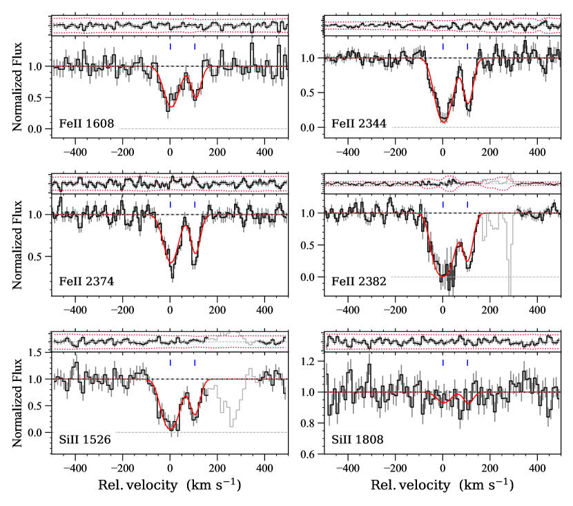
Figure 7: Voigt profile fits to the low-ionisation metal absorption lines of the $z=2.6773$ DLA towards Q 0139–0824. Each panel shows the continuum normalised flux of a single transition (bottom), and the fit residuals (top). The black line represents the observed spectrum with uncertainties shown as grey vertical bars. Grey regions without uncertainties were excluded in the fit. The red curve represents the best fit.

References

- Abbott et al. (2000) Abbott T. M., et al., 2000, in Iye M., Moorwood A. F., eds, Proc. SPIEVol. 4008, Optical and IR Telescope Instrumentation and Detectors. pp 714–719, doi:10.1117/12.395528
- Arnouts et al. (1999) Arnouts S., Cristiani S., Moscardini L., Matarrese S., Lucchin F., Fontana A., Giallongo E., 1999, MNRAS, 310, 540
- Asplund et al. (2009) Asplund M., Grevesse N., Sauval A. J., Scott P., 2009, ARA&A, 47, 481
- Astropy Collaboration et al. (2013) Astropy Collaboration et al., 2013, A&A, 558, A33
- Augustin et al. (2018) Augustin R., et al., 2018, MNRAS, 478, 3120
- Bashir et al. (2019) Bashir W., Zafar T., Khan F. M., Chishtie F., 2019, New Astronomy, 66, 9
- Berg et al. (2016) Berg T. A. M., et al., 2016, MNRAS, 463, 3021
- Berry et al. (2016) Berry M., Somerville R. S., Gawiser E., Maller A. H., Popping G., Trager S. C., 2016, MNRAS, 458, 531
- Bouché et al. (2012) Bouché N., et al., 2012, MNRAS, 419, 2
- Bouché et al. (2013) Bouché N., Murphy M. T., Kacprzak G. G., Péroux C., Contini T., Martin C. L., Dessauges-Zavadsky M., 2013, Science, 341, 50
- Bradley et al. (2016) Bradley L., et al., 2016, Photutils: Photometry tools, Astrophysics Source Code Library (ascl:1609.011)
- Bruzual & Charlot (2003) Bruzual G., Charlot S., 2003, MNRAS, 344, 1000
- Calzetti et al. (2000) Calzetti D., Armus L., Bohlin R. C., Kinney A. L., Koornneef J., Storchi-Bergmann T., 2000, ApJ, 533, 682
- Cappetta et al. (2010) Cappetta M., D’Odorico V., Cristiani S., Saitta F., Viel M., 2010, MNRAS, 407, 1290
- Cashman et al. (2017) Cashman F. H., Kulkarni V. P., Kisielius R., Ferland G. J., Bogdanovich P., 2017, ApJS, 230, 8
- Chabrier (2003) Chabrier G., 2003, PASP, 115, 763
- Christensen et al. (2014) Christensen L., Møller P., Fynbo J. P. U., Zafar T., 2014, MNRAS, 445, 225
- Crighton et al. (2015) Crighton N. H. M., et al., 2015, MNRAS, 452, 217
- De Cia et al. (2016) De Cia A., Ledoux C., Mattsson L., Petitjean P., Srianand R., Gavignaud I., Jenkins E. B., 2016, A&A, 596, A97
- Fynbo et al. (1999) Fynbo J. U., Møller P., Warren S. J., 1999, MNRAS, 305, 849
- Fynbo et al. (2008) Fynbo J. P. U., Prochaska J. X., Sommer-Larsen J., Dessauges-Zavadsky M., Møller P., 2008, ApJ, 683, 321
- Fynbo et al. (2010) Fynbo J. P. U., et al., 2010, MNRAS, 408, 2128
- Fynbo et al. (2011) Fynbo J. P. U., et al., 2011, MNRAS, 413, 2481
- Fynbo et al. (2013) Fynbo J. P. U., et al., 2013, MNRAS, 436, 361
- Hartoog et al. (2015) Hartoog O. E., Fynbo J. P. U., Kaper L., De Cia A., Bagdonaite J., 2015, MNRAS, 447, 2738
- Hayes et al. (2010) Hayes M., et al., 2010, Nature, 464, 562
- Hunter (2007) Hunter J. D., 2007, Computing In Science & Engineering, 9, 90
- Ilbert et al. (2006) Ilbert O., et al., 2006, A&A, 457, 841
- Jorgenson & Wolfe (2014) Jorgenson R. A., Wolfe A. M., 2014, ApJ, 785, 16
- Kanekar et al. (2018) Kanekar N., et al., 2018, ApJ, 856, L23
- Kashikawa et al. (2014) Kashikawa N., Misawa T., Minowa Y., Okoshi K., Hattori T., Toshikawa J., Ishikawa S., Onoue M., 2014, ApJ, 780, 116
- Kennicutt (1998) Kennicutt Robert C. J., 1998, ARA&A, 36, 189
- Kochiashvili et al. (2015) Kochiashvili I., et al., 2015, A&A, 580, A42
- Komatsu et al. (2011) Komatsu E., et al., 2011, ApJS, 192, 18
- Krogager (2018) Krogager J.-K., 2018, arXiv e-prints, p. arXiv:1803.01187
- Krogager et al. (2012) Krogager J.-K., Fynbo J. P. U., Møller P., Ledoux C., Noterdaeme P., Christensen L., Milvang-Jensen B., Sparre M., 2012, MNRAS, 424, L1
- Krogager et al. (2013) Krogager J.-K., et al., 2013, MNRAS, 433, 3091
- Krogager et al. (2017) Krogager J.-K., Møller P., Fynbo J. P. U., Noterdaeme P., 2017, MNRAS, 469, 2959
- Kulkarni et al. (2000) Kulkarni V. P., Hill J. M., Schneider G., Weymann R. J., Storrie-Lombardi L. J., Rieke M. J., Thompson R. I., Jannuzi B. T., 2000, ApJ, 536, 36
- Laursen et al. (2009) Laursen P., Razoumov A. O., Sommer-Larsen J., 2009, ApJ, 696, 853
- Livermore et al. (2015) Livermore R. C., et al., 2015, MNRAS, 450, 1812
- Lopez et al. (2002) Lopez S., Reimers D., D’Odorico S., Prochaska J. X., 2002, A&A, 385, 778
- López et al. (2016) López S., et al., 2016, A&A, 594, A91
- Modigliani et al. (2010) Modigliani A., et al., 2010, in Observatory Operations: Strategies, Processes, and Systems III. p. 773728, doi:10.1117/12.857211
- Møller & Christensen (2020) Møller P., Christensen L., 2020, MNRAS, 492, 4805
- Møller et al. (2002) Møller P., Warren S. J., Fall S. M., Fynbo J. U., Jakobsen P., 2002, ApJ, 574, 51
- Møller et al. (2013) Møller P., Fynbo J. P. U., Ledoux C., Nilsson K. K., 2013, MNRAS, 430, 2680
- Møller et al. (2018) Møller P., et al., 2018, MNRAS, 474, 4039
- Noterdaeme et al. (2012) Noterdaeme P., et al., 2012, A&A, 547, L1
- Peng et al. (2002) Peng C. Y., Ho L. C., Impey C. D., Rix H.-W., 2002, AJ, 124, 266
- Péroux et al. (2003) Péroux C., Dessauges-Zavadsky M., D’Odorico S., Kim T.-S., McMahon R. G., 2003, MNRAS, 345, 480
- Péroux et al. (2012) Péroux C., Bouché N., Kulkarni V. P., York D. G., Vladilo G., 2012, MNRAS, 419, 3060
- Prochaska et al. (2003) Prochaska J. X., Gawiser E., Wolfe A. M., Castro S., Djorgovski S. G., 2003, ApJ, 595, L9
- Prochaska et al. (2005) Prochaska J. X., Herbert-Fort S., Wolfe A. M., 2005, ApJ, 635, 123
- Rafelski et al. (2014) Rafelski M., Neeleman M., Fumagalli M., Wolfe A. M., Prochaska J. X., 2014, ApJ, 782, L29
- Rhodin et al. (2018) Rhodin N. H. P., Christensen L., Møller P., Zafar T., Fynbo J. P. U., 2018, A&A, 618, A129
- Rhodin et al. (2019) Rhodin N. H. P., Agertz O., Christensen L., Renaud F., Fynbo J. P. U., 2019, MNRAS, 488, 3634
- STSCI Development Team (2012) STSCI Development Team 2012, DrizzlePac: HST image software, Astrophysics Source Code Library (ascl:1212.011)
- Sánchez-Ramírez et al. (2016) Sánchez-Ramírez R., et al., 2016, MNRAS, 456, 4488
- Schlafly & Finkbeiner (2011) Schlafly E. F., Finkbeiner D. P., 2011, ApJ, 737, 103
- Verhamme et al. (2008) Verhamme A., Schaerer D., Atek H., Tapken C., 2008, A&A, 491, 89
- Vernet et al. (2011) Vernet J., et al., 2011, A&A, 536, A105
- Warren et al. (2001) Warren S. J., Møller P., Fall S. M., Jakobsen P., 2001, MNRAS, 326, 759
- Weatherley et al. (2005) Weatherley S. J., Warren S. J., Møller P., Fall S. M., Fynbo J. U., Croom S. M., 2005, MNRAS, 358, 985
- Wenger et al. (2000) Wenger M., et al., 2000, A&AS, 143, 9
- Whitaker et al. (2014) Whitaker K. E., et al., 2014, ApJ, 795, 104
- Whitaker et al. (2015) Whitaker K. E., et al., 2015, ApJ, 811, L12
- Wolfe et al. (1986) Wolfe A. M., Turnshek D. A., Smith H. E., Cohen R. D., 1986, ApJS, 61, 249
- Wolfe et al. (2008) Wolfe A. M., Prochaska J. X., Jorgenson R. A., Rafelski M., 2008, ApJ, 681, 881
- Zafar et al. (2013) Zafar T., Popping A., Péroux C., 2013, A&A, 556, 140
- Zafar et al. (2017) Zafar T., Møller P., Péroux C., Quiret S., Fynbo J. P. U., Ledoux C., Deharveng J.-M., 2017, MNRAS, 465, 1613
- van der Wel et al. (2014) van der Wel A., et al., 2014, ApJ, 788, 28