Exterior-point Optimization for Sparse and Low-rank Optimization

Abstract

In this paper we present the nonconvex exterior-point optimization solver (NExOS)—a first-order algorithm tailored to constrained nonconvex optimization problems. We consider the problem of minimizing a convex function over nonconvex constraints, where the projection onto the constraint set is single-valued around local minima. A wide range of nonconvex optimization problems have this structure including (but not limited to) sparse and low-rank optimization problems. By exploiting the underlying geometry of the constraint set, NExOS finds a locally optimal point by solving a sequence of penalized problems with strictly decreasing penalty parameters. NExOS solves each penalized problem by applying a first-order algorithm, which converges linearly to a local minimum of the corresponding penalized formulation under regularity conditions. Furthermore, the local minima of the penalized problems converge to a local minimum of the original problem as the penalty parameter goes to zero. We then implement and test NExOS on many instances from a wide variety of sparse and low-rank optimization problems. We demonstrate that our algorithm, outperforms specialized methods on several examples of well-known nonconvex optimization problems involving sparse and low-rank optimization.

1 Introduction

This paper studies optimization problems involving a strongly convex and smooth cost function over a closed nonconvex constraint set $\mathcal{X}$. We propose a first-order algorithm nonconvex exterior-point optimization solver (NExOS) to solve such problems numerically. We can write such problems as:

$$\begin{array}[]{ll}\underset{}{\mbox{minimize}}&f(x)+(\beta/2)\|x\|^{2}\\ \textrm{subject to}&x\in\mathcal{X},\end{array} \mathcal{P}$$ ()

where $x$ takes value in a finite-dimensional vector space $\mathbf{E}$ over the reals, $f$ is a strongly convex and smooth function. The regularization parameter $\beta>0$ is commonly introduced to reduce the generalization error without increasing the training error (Goodfellow-et-al-2016, , §5.2.2). Furthermore, $\mathbf{E}$ is equipped with inner product $\left\langle\cdot\mid\cdot\right\rangle$ and norm $\|\cdot\|=\sqrt{\left\langle x\mid x\right\rangle}$. The constraint set $\mathcal{X}$ is closed, potentially nonconvex, but prox-regular at local minima, i.e., it has single-valued Euclidean projection around local minima PoliRocka2000 . In many practical applications (see §1.1), the constraint set $\mathcal{X}$ decomposes as $\mathcal{X}=\text{$\mathcal{C}$}\bigcap\mathcal{N}$, where $\mathcal{C}$ is a compact convex set, and $\mathcal{N}$ is prox-regular around local minima; in this case the feasible set $\mathcal{X}$ inherits the prox-regularity property around local minima from the set $\mathcal{N}$ (see Lemma 3 in §3) .

Definition 1 (Prox-regular set PoliRocka2000 ).

A nonempty closed set $\mathcal{S}\subseteq\mathbf{E}$ is prox-regular at a point $x\in\mathcal{S}$ if projection onto $\mathcal{S}$ is single-valued on a neighborhood of $x$. The set $\mathcal{S}$ is prox-regular if it is prox-regular at every point in the set.

In Appendix B.1, we generalize our framework to the case when $f$ is non-smooth convex.

1.1 Applications

Among prox-regular sets, sparse and low-rank constraint sets are perhaps the most prominent in machine learning because they allow for high interpretability, speed-ups in computation, and reduced memory requirements jain2017non .

Low-rank optimization

We can write low-rank optimization problems in the form ($\mathcal{P}$), which are common in machine learning applications such as collaborative filtering (jain2017non, , pp. 279-281), design of online recommendation systems Mazumder2010 ; Candes2009 , bandit optimization jun2019bilinear , data compression Gress2014 ; Mikolov2013 ; Srikumar2014 , and low rank kernel learning Bach2013 . In these applications, the constraint set $\mathcal{X}$ decomposes as $\mathcal{X}=\text{$\mathcal{C}$}\bigcap\mathcal{N}$, where $\mathcal{C}$ is a compact convex set, and

$$\mathcal{N}=\{X\in\mbox{{\bf R}}^{m\times d}\mid\mathop{{\bf rank}}(X)\leq r\},$$ (1)

which is prox-regular at any point $X\in\mathbf{R}^{m\times d}$ where $\mathop{{\bf rank}}(X)=r$ (Luke2013, , Proposition 3.8). One can show that $\mathcal{X}$ inherits the prox-regularity property at any $X$ with $\mathop{{\bf rank}}(X)=r$ from the set $\mathcal{N}$; a formal proof is given in Lemma 3 in Appendix A.1. In this paper, we apply NExOS to solve the affine rank minimization problem:

$$\begin{array}[]{ll}\textup{minimize}&\left\|\mathcal{A}(X)-b\right\|_{2}^{2}+(\beta/2)\|X\|_{F}^{2}\\ \textup{subject to}&\mathop{{\bf rank}}(X)\leq r,\quad\|X\|_{2}\leq\Gamma,\end{array}$$ (RM)

where $X\in\mathbf{R}^{m\times d}$ is the decision variable, $b\in\mathbf{R}^{k}$ is noisy measurement data, and $\mathcal{A}:\mathbf{R}^{m\times d}\to\mathbf{R}^{k}$ is a linear map. The parameter $\Gamma>0$ is the upper bound for the spectral norm of $X$. The affine map $\mathcal{A}$ is determined by $k$ matrices $A_{1},\ldots,A_{k}$ in $\mathbf{R}^{m\times d}$ where $\mathcal{A}(X)=(\mathbf{tr}(A_{1}^{T}X),\ldots,\mathbf{tr}(A_{k}^{T}X)).$ We present several numerical experiments to solve (RM) using NExOS for both synthetic and real-world datasets in §4.2.

Sparsity-constrained optimization

Sparsity constraints have found applications in many practical settings, e.g., gene expression analysis (Hastie2015, , pp. 2–4), sparse regression (jain2017non, , pp. 155–157), signal transmission and recovery Candes2008 ; Tropp2006 , hierarchical sparse polynomial regression Bertsimas2020 , and best subset selection bertsimas2016best , just to name a few. In these problems, the constraint set $\mathcal{X}$ decomposes as $\mathcal{X}=\text{$\mathcal{C}$}\bigcap\mathcal{N}$, where $\mathcal{C}$ is a compact convex set, and

$$\mathcal{N}=\{x\in\mbox{{\bf R}}^{d}\mid\mathop{{\bf card}}(x)\leq k\},$$ (2)

where $\mathbf{card}(x)$ counts the number of nonzero elements in $x$. Similarly, $\mathcal{N}$ in (2) is prox-regular at any point $x$ satisfying $\mathop{{\bf card}}(x)=k$ because we can write $\mathbf{card}(x)\leq k$ as a special case of the low-rank constraint by embedding the components of $x$ in the diagonal entries of a matrix and then using the prox-regularity of low-rank constraint set. In this paper, we apply NExOS to solve the sparse regression problem for both synthetic and real-world datasets in §4.1, which is concerned with approximating a vector $b\in\mathbf{R}^{m}$ with a linear combination of at most $k$ columns of a matrix $A\in\mathbf{R}^{m\times d}$ with bounded coefficients. This problem has the form:

$$\begin{array}[]{ll}\textup{minimize}&\|Ax-b\|_{2}^{2}+(\beta/2)\|x\|_{2}^{2}\\ \textup{subject to}&\mathbf{card}(x)\leq k,\quad\|x\|_{\infty}\leq\Gamma,\end{array}$$ (SR)

where $x\in\mathbf{R}^{d}$ is the decision variable, and $A\in\mathbf{R}^{m\times d},\;b\in\mathbf{R}^{m},$ and $\Gamma>0$ are problem data.

Some other notable prox-regular sets are as follows. Closed convex sets are prox-regular everywhere (Rockafellar2009, , page 612). Examples of well-known prox-regular sets that are not convex include sets involving bilinear constraints bauschke2022projections , weakly convex sets vial1983strong , proximally smooth sets clarke1995proximal , strongly amenable sets (Rockafellar2009, , page 612), and sets with Shapiro property shapiro1994existence . Also, a nonconvex set defined by a system of finitely many inequality and equality constraints for which a basic constraint qualification holds is prox-regular (rockafellar2020characterizing, , page 10).

1.2 Related work

Due to the presence of the nonconvex set $\mathcal{X},$ the nonconvex problem ($\mathcal{P}$) is $\mathcal{NP}$-hard Hardt2014 . A common way to deal with this issue is to avoid this inherent nonconvexity altogether by convexifying the original problem. The relaxation of the sparsity constraint leads to the popular LASSO formulation and its variants Hastie2015 , whereas relaxation of the low-rank constraints produces the nuclear norm based convex models Fazel2008 . The basic advantage of the convex relaxation technique is that, in general, a globally optimal solution to a convex problem can be computed reliably and efficiently (boyd2004convex, , §1.1), whereas for nonconvex problems a local optimal solution is often the best one can hope for. Furthermore, if certain statistical assumptions on the data generating process hold, then it is possible to recover exact solutions to the original nonconvex problems with high probability by solving the convex relaxations (see Hastie2015 and the references therein). However, when stringent assumptions do not hold, then solutions to the convex formulations can be of poor quality and may not scale very well (jain2017non, , §6.3 and §7.8). In this situation, the nonconvexity of the original problem must be confronted directly, because such nonconvex formulations capture the underlying problem structures more accurately than their convex counterparts.

To that goal, first-order algorithms such as hard thresholding algorithms, e.g., IHT blumensath2008iterative , NIHT blumensath2010normalized , HTP foucart2011hard , CGIHT blanchard2015cgiht , address nonconvexity in sparse and low-rank optimization by implementing variants of projected gradient descent with projection taken onto the sparse and/or low-rank set. While these algorithms have been successful in recovering low-rank and sparse solutions in underdetermined linear systems, they too require assumptions on the data such as the restricted isometry property for recovering true solutions (jain2017non, , §7.5). Furthermore, to converge to a local minimum, hard thresholding algorithms require the spectral norm of the measurement matrix to be less than one, which is a restrictive condition blumensath2008iterative . Besides hard thresholding algorithms, heuristics based on first-order algorithms such as the alternating direction method of multipliers (ADMM) have gained a lot of traction in the last few years. Though ADMM was originally designed to solve convex optimization problems, since the idea of implementing this algorithm as a general purpose heuristic to solve nonconvex optimization problems was introduced in (Boyd2011, , §9.1-9.2), ADMM-based heuristics have been applied successfully to approximately solve nonconvex problems in many different application areas Takapoui2017 ; Diamond2018 . However, the biggest drawback of these heuristics comes from the fact that they take an algorithm designed to solve convex problems and apply it verbatim to a nonconvex setup. As a result, these algorithms often fail to converge, and even when they do, it need not be a local minimum, let alone a global one (Takapoui2017a, , §2.2). Also, empirical evidence suggests that the iterates of these algorithms may diverge even if they come arbitrarily close to a locally optimal solution during some iteration. The main reason is that these heuristics do not establish a clear relationship between the local minimum of ($\mathcal{P}$) and the fixed point set of the underlying operator that controls the iteration scheme. An alternative approach that has been quite successful empirically in finding low-rank solutions is to consider an unconstrained problem with Frobenius norm penalty and then using alternating minimization to compute a solution UdellGlrm . However, the alternating minimization approach may not converge to a solution and should be considered a heuristic (UdellGlrm, , §2.4).

For these reasons above, in the last few years, there has been significant interest in addressing the nonconvexity present in many optimization problems directly via a discrete optimization approach. In this way, a particular nonconvex optimization problem is formulated exactly using discrete optimization techniques and then specialized algorithms are developed to find a certifiably optimal solution. This approach has found considerable success in solving machine learning problems with sparse and low-rank optimization BertsimasMLLens ; tillmann2021cardinality . A mixed integer optimization approach to compute near-optimal solutions for sparse regression problem, where problem dimension $d=1000$, is computed in bertsimas2016best . In bertsimas2020sparse , the authors propose a cutting plane method for a similar problem, which works well with mild sample correlations and a sufficiently large dimension. In hazimeh2020fast , the authors design and implement fast algorithms based on coordinate descent and local combinatorial optimization to solve sparse regression problem with a three-fold speedup where $d\approx 10^{6}$. In bertsimas2020mixed , the authors propose a framework for modeling and solving low-rank optimization problems to certifiable optimality via symmetric projection matrices. However, the runtime of these algorithms can often become prohibitively long as the problem dimensions grow bertsimas2016best . Also, these discrete optimization algorithms have efficient implementations only for a narrow class of loss functions and constraint sets; they do not generalize well if a minor modification is made to the problem structure, and in such a case they often fail to find a solution point in a reasonable amount of time even for smaller dimensions BertsimasMLLens . Furthermore, one often relies on commercial softwares, such as Gurobi, Mosek, or Cplex to solve these discrete optimization problems, thus making the solution process somewhat opaque bertsimas2016best ; tillmann2021cardinality .

1.3 Contributions

The main contribution of this work is to propose NExOS: a first-order algorithm tailored for nonconvex optimization problems of the form ($\mathcal{P}$). The term exterior-point originates from the fact that the iterates approach a local minimum from outside of the feasible region; it is inspired by the convex exterior-point method first proposed by Fiacco and McCormick in the 1960s (fiacco1990nonlinear, , §4). By exploiting the prox-regularity of the constraint set, we construct an iterative method that finds a locally optimal point of the original problem via an outer loop consisting of increasingly accurate penalized formulations of the original problem by reducing only one penalty parameter. Each penalized problem is then solved by applying an inner algorithm that implements a variant of the Douglas-Rachford splitting algorithm.

We prove that NExOS, besides avoiding the drawbacks of convex relaxation and discrete optimization approach, has the following favorable features. First, the penalized problem has strong convexity and smoothness around local minima, but can be made arbitrarily close to the original nonconvex problem by reducing the penalty parameter. Second, under mild regularity conditions, the inner algorithm finds local minima for the penalized problems at a linear convergence rate, and as the penalty parameter goes to zero, the local minima of the penalized problems converge to a local minimum of the original problem. Furthermore, we show that, when those regularity conditions do not hold, the inner algorithm is still guaranteed to subsequentially converge to a first-order stationary point of the penalized problem at the rate $o(1/\sqrt{k})$.

We implement NExOS in the open-source Julia package NExOS.jl and test it extensively on many synthetic and real-world instances of different nonconvex optimization problems of substantial current interest. We demonstrate that NExOS very quickly computes solutions that are competitive with or better than specialized algorithms on various performance measures. NExOS.jl is available at https://github.com/Shuvomoy/NExOS.jl.

Organization of the paper

The rest of the paper is organized as follows. We describe our NExOS framework in §2. We provide convergence analysis of the algorithm in §3. Then we demonstrate the performance of our algorithm on several nonconvex optimization problems of significant current interest in §4. The concluding remarks are presented in §5.

Notation and notions

Domain of a function $h:\mathbf{E}\to\mbox{{\bf R}}\cup\{\infty\}$ is defined as $\mathop{{\bf dom}}h=\{x\in\mathbf{E}\mid h(x)<\infty\}$. A function $f$ is proper if its domain is nonempty, and it is lower-semicontinuous if its epigraph $\mathop{{\bf epi}}f=\{(x,t)\in\mathbf{E}\times\mbox{{\bf R}}\mid f(x)\leq t\}$ is a closed set. By $B(x;r)$ and $\overline{B}(x;r)$, we denote an open ball and a closed ball of radius $r$ and center $x$, respectively. A set-valued operator $\mathbb{A}:\mathbf{E}\rightrightarrows\mathbf{E}$ maps an element $x$ in $\mathbf{E}$ to a set $\mathbb{A}(x)$ in $\mathbf{E}$; its domain is defined as $\mathop{{\bf dom}}\mathbb{A}=\{x\in\mathbf{E}\mid\mathbb{A}(x)\neq\emptyset\},$ its range is defined as $\mathop{{\bf ran}}\mathbb{A}=\bigcup_{x\in\mathbf{E}}\mathbb{A}(x),$ and it is completely characterized by its graph: $\mathop{{\bf gra}}\mathbb{A}=\{(u,x)\in\mathbf{E}\times\mathbf{E}\mid u\in\mathbb{A}(x)\}.$ Furthermore, we define $\mathop{\mathop{{\bf fix}}}\mathbb{A}=\{x\in\mathbf{E}\mid x\in\mathbb{A}(x)\},$ and $\mathop{{\bf zer}}\mathbb{A}=\{x\in\mathbf{E}\mid 0\in\mathbb{A}(x)\}.$ For every $x,$ addition of two operators $\mathbb{A}_{1},\mathbb{A}_{2}:\mathbf{E}\rightrightarrows\mathbf{E}$, denoted by $\mathbb{A}_{1}+\mathbb{A}_{2}$, is defined as $(\mathbb{A}_{1}+\mathbb{A}_{2})(x)=\mathbb{A}_{1}(x)+\mathbb{A}_{2}(x),$ subtraction is defined analogously, and composition of these operators, denoted by $\mathbb{A}_{1}\mathbb{A}_{2},$ is defined as $\mathbb{A}_{1}\mathbb{A}_{2}(x)=\mathbb{A}_{1}(\mathbb{A}_{2}(x))$; note that order matters for composition. Also, if $\mathcal{S}\subseteq\mathbf{E}$ is a nonempty set, then $\mathbb{A}(\mathcal{S})=\cup\{\mathbb{A}(x)\mid x\in\mathcal{S}\}$. An operator $\mathbb{A}:\mathbf{E}\to\mathbf{E}$ is nonexpansive on some set $\mathcal{S}$ if it is Lipschitz continuous with Lipschitz constant $1$ on $\mathcal{S}$; the operator is contractive if the Lipschitz constant is strictly smaller than $1$. On the other hand, $\mathbb{A}$ is firmly nonexpansive on $\mathcal{S}$ if and only if its reflection operator $2\mathbb{A}-\mathbb{I}$ is nonexpansive on $\mathcal{S}$. A firmly nonexpansive operator is always nonexpansive (Bauschke2017, , page 59).

2 Our approach

The backbone of our approach is to address the nonconvexity by working with an asymptotically exact nonconvex penalization of ($\mathcal{P}$), which enjoys local convexity around local minima. We use the notation $\iota(x)$ that denotes the indicator function of the set $\mathcal{X}$ at $x$, which is $0$ if $x\in\mathcal{X}$ and $\infty$ else. Using this, we can write ($\mathcal{P}$) as an unconstrained optimization problem, where the objective is $f(x)+(\beta/2)\|x\|^{2}+\iota(x)$. In our penalization, we replace the indicator function $\iota$ with its Moreau envelope with positive parameter $\mu$:

$$\prescript{\mu}{}{\iota}(x) =\min_{y}\{\iota(y)+(1/2\mu)\|y-x\|^{2}\}=(1/2\mu)d^{2}(x),$$ (3)

where $d(x)$ is the Euclidean distance of the point $x$ from the set $\mathcal{X}$. While $\prescript{\mu}{}{\iota}$ is still nonconvex, the main benefit of working with it is that, it is (i) finite and bounded on bounded sets, (ii) jointly continuous in $\mu$ and $x$, (iii) a global underestimator of the indicator function $\iota$, which improves with decreasing $\mu$ and becomes asymptotically equal to $\iota$ as $\mu$ approaches 0, and (iv) for any value of $\beta>0$ and $0<\mu\leq(1/\beta)$ the function $\prescript{\mu}{}{\iota}+(\beta/2)\|\cdot\|^{2}$ is convex and differentiable on a neighborhood around local minima. See (Bauschke2017, , Proposition 12.9) for the first three properties, and Proposition 1 in §3 for the last one. The favorable features of $\prescript{\mu}{}{\iota}$ motivate us to consider the following penalization formulation of ($\mathcal{P}$):

$$\begin{array}[]{ll}\textup{minimize}&f(x)+\prescript{\mu}{}{\bbiota}(x),\end{array} \mathcal{P}_{\mu}$$ ()

where $\prescript{\mu}{}{\bbiota}\equiv\prescript{\mu}{}{\iota}+(\beta/2)\|\cdot\|^{2}$, $x\in\mathbf{E}$ is the decision variable, and $\mu$ is a positive penalty parameter. We call the cost function in ($\mathcal{P}_{\mu}$) an exterior-point minimization function; the term is inspired by (fiacco1990nonlinear, , §4.1). The notation $\prescript{\mu}{}{\bbiota}\equiv\prescript{\mu}{}{\iota}+(\beta/2)\|\cdot\|^{2}$ introduced in ($\mathcal{P}_{\mu}$) not only reduces notational clutter, but also alludes to a specific way of splitting the objective into two summands $f$ and $\prescript{\mu}{}{\bbiota}$, which will ultimately allow us to establish convergence of our algorithm in §3. Because $\prescript{\mu}{}{\iota}$ is an asymptotically exact approximation of $\iota$ as $\mu\to 0$, solving ($\mathcal{P}_{\mu}$) for a small enough value of the penalty parameter $\mu$ suffices for all practical purposes. Now that we have intuitively justified the exact penalization ($\mathcal{P}_{\mu}$), we are in a position to present our algorithm.

   given: regularization parameter $\beta>0$, an initial point $z_{\textup{init}}$, initial penalty parameter $\mu_{\textup{init}}$, minimum penalty parameter $\mu_{\textup{min}}$, tolerance for the fixed point gap $\epsilon$ for each inner iteration, tolerance for stopping criterion $\delta$ for the outer iteration, and multiplicative factor $\rho\in(0,1)$.

 Initialization. $\mu\coloneqq\mu_{\textup{init}}$, and $z^{0}\coloneqq z_{\textup{init}}$.

Outer iteration. while stopping criterion is not met do

       Inner iteration. Using Algorithm 2, compute $x_{\mu},y_{\mu}$, and $z_{\mu}$ that solve $(\mathcal{P}_{\mu})$ with tolerance $\epsilon$, where $z_{\mu}^{0}\coloneqq z^{0}$ is input as the initial point.

       Stopping criterion. quit if $\lvert\left(f(\mathop{{\bf\Pi}}x_{\mu})+(\beta/2)\|\mathbf{\Pi}x_{\mu}\|^{2}\right)-\left(f(x_{\mu})+\prescript{\mu}{}{\bbiota}(x_{\mu})\right)\rvert\leq\delta$.

      Set initial point for next inner iteration. $z^{0}\coloneqq z_{\mu}$.

       Update $\mu$. $\mu\coloneqq\rho\mu$.

end while

return $x_{\mu},y_{\mu},$ and $z_{\mu}$

  

Algorithm 1 Nonconvex Exterior-point Optimization Solver (NExOS). Here $\mathop{{\bf\Pi}}(x)$ denotes the Euclidean projection of $x$ on the nonconvex set $\mathcal{X}$

   given: starting point $z^{0}$, tolerance for the fixed point gap $\epsilon$, and proximal parameter $\gamma>0$.

Initialization. $n\coloneqq 0$, $\kappa\coloneqq 1/(\beta\gamma+1)$, $\theta\coloneqq\mu/(\gamma\kappa+\mu)$.

while $\|x^{n}-y^{n}\|>\epsilon$  do

       Compute $x^{n+1}\coloneqq\mathbf{prox}_{\gamma f}\left(z^{n}\right)$.

       Compute $\tilde{y}^{n+1}\coloneqq\kappa\left(2x^{n+1}-z^{n}\right)$.

       Compute $y^{n+1}\coloneqq\theta\tilde{y}^{n+1}+\left(1-\theta\right)\mathop{{\bf\Pi}}\left(\tilde{y}^{n+1}\right)$.

       Compute $z^{n+1}\coloneqq z^{n}+y^{n+1}-x^{n+1}$.

       Update $n\coloneqq n+1$.

end while

return $x^{n},y^{n},$ and $z^{n}$.

  

Algorithm 2 Inner Algorithm for ($\mathcal{P}_{\mu}$). Here $\mathop{{\bf\Pi}}(x)$ denotes the Euclidean projection of $x$ on the nonconvex set $\mathcal{X}$, and $\mathbf{prox}_{\gamma f}$ denotes the proximal operator of $f$ with parameter $\gamma>0$ as defined in (4).

Algorithm description

Algorithm 1 outlines NExOS. The main part is an outer loop that solves a sequence of penalized problems of the form ($\mathcal{P}_{\mu}$) with strictly decreasing penalty parameter $\mu$, until the termination criterion is met, at which point the exterior-point minimization function is a sufficiently close approximation of the original cost function. For each $\mu$, ($\mathcal{P}_{\mu}$) is solved by an inner algorithm, denoted by Algorithm 2. One can derive Algorithm 2 by applying Douglas-Rachford splitting (DRS) (Bauschke2017, , page 401) to ($\mathcal{P}_{\mu}$), this derivation is deferred to Appendix A.2.

Algorithm subroutines

The inner algorithm requires two subroutines, evaluating (i) $\mathbf{prox}_{\gamma f}(x)$, which is the proximal operator of the convex function $f$ at the input point $x$, and (ii) $\mathop{{\bf\Pi}}(x)$, which is a projection of $x$ on the nonconvex set $\mathcal{X}$. We discuss now how we compute them in our implementation. To that goal, we recall that, for a function $g$ (not necessarily convex) its proximal operator $\mathbf{prox}_{\gamma g}$ and Moreau envelope $\prescript{\gamma}{}{f}$, where $\gamma>0$, are defined as:

$$\mathbf{prox}_{\gamma g}(x)=\mathop{\textrm{argmin}}_{y\in\mathbf{E}}\left(g(y)+(1/2\gamma)\|y-x\|^{2}\right),$$ (4)

$$\prescript{\gamma}{}{g}(x)=\textrm{min}_{y\in\mathbf{E}}\left(g(y)+(1/2\gamma)\|y-x\|^{2}\right).$$

Computing proximal operator of $f$

For the convex function $f$, $\mathbf{prox}_{\gamma f}$ is always single-valued and computing it is equivalent to solving a convex optimization problem, which often can be done in closed form for many relevant cost functions in machine learning (beck2017first, , pp. 449-450). If the proximal operator of $f$ does not admit a closed form solution, then we solve the corresponding convex optimization problem (4) to a high precision solution. For this purpose, we can select any convex optimization solver supported by MathOptInterface, which is the abstraction layer for optimization solvers in Julia.

Computing projection onto $\mathcal{X}$

The notation $\mathop{{\bf\Pi}}(x)$ denotes the projection operator of $x$ onto the constraint set $\mathcal{X}$, defined as $\mathbf{\Pi}(x)=\mathbf{prox}_{\gamma\iota}(x)=\textrm{argmin}_{y\in\mathcal{X}}(\|y-x\|^{2}).$ A list of nonconvex sets that are easy to project onto can be found in (Diamond2018, , §4), this includes nonconvex sets such as boolean vectors with fixed cardinality, vectors with bounded cardinality, quadratic sets, matrices with bounded singular values, matrices with bounded rank etc. If $\mathcal{X}$ is in this list, then we project onto $\mathcal{X}$ directly.

Now consider the case where the constraint set $\mathcal{X}$ decomposes as $\mathcal{X}=\text{$\mathcal{C}$}\bigcap\mathcal{N}$, where $\mathcal{N}$ is a nonconvex set with tractable projection and $\mathcal{C}$ is any compact convex set. In this setup, let $\mathcal{\iota}_{\mathcal{C}}$ and $\iota_{\mathcal{N}}$ be the indicator functions of $\mathcal{C}$ and $\mathcal{N}$, respectively. Defining $\phi=f+\mathcal{\iota}_{\mathcal{C}}$, we write ($\mathcal{P}$) as: $\min_{x\in\mathbf{E}}\phi(x)+(\beta/2)\|x\|^{2}+\iota_{\mathcal{N}}(x).$ For any convex function $\phi$, its Moreau envelope $\prescript{\nu}{}{\phi}$, for any $\nu>0$, has the following three desirable features. First, for every $x\in\mathbf{E}$ we have $\prescript{\nu}{}{\phi}(x)\leq\phi(x)$ and $\prescript{\nu}{}{\phi}(x)\to\phi(x)$ as $\nu\to 0$ (Rockafellar2009, , Theorem 1.25). Second, we have $x^{\star}\in\mathop{\textrm{argmin}}_{x\in\mathbf{E}}\phi(x)$ if and only if $x^{\star}\in\mathop{\textrm{argmin}}_{x\in\mathbf{E}}\prescript{\nu}{}{\phi}(x)$ with the minimizer $x^{\star}$ satisfying $\phi(x^{\star})=\prescript{\nu}{}{\phi}(x^{\star})$ (Bauschke2017, , Corollary 17.5). Third, the Moreau envelope $\prescript{\nu}{}{\phi}$ is convex, and smooth (i.e., it is differentiable and its gradient is Lipschitz continuous) everywhere irrespective of the differentiability or smoothness of the original function $\phi$. The gradient is: $\prescript{\nu}{}{\phi}(x)=\left(x-\mathbf{prox}_{\nu\phi}(x)\right)/\nu,$ which is $(1/\nu)-$Lipschitz continuous (Bauschke2017, , Proposition 12.29). These properties make $\prescript{\nu}{}{\phi}$ a smooth approximation of $\phi$ for a small enough $\nu$. Hence, we work with the following approximation of the original problem: $\min_{x}\prescript{\nu}{}{\phi}+(\beta/2)\|x\|^{2}+\iota_{\mathcal{N}}(x),$ where we replace $f$ with $\prescript{\nu}{}{\phi}$ and $\iota$ with $\iota_{\mathcal{N}}$ in Algorithms 1 and 2. The proximal operator of $\prescript{\nu}{}{\phi}$ can be computed using $\mathbf{prox}_{\gamma\prescript{\nu}{}{\phi}}(x)=x+(\gamma/(\gamma+\nu))(\mathbf{prox}_{(\gamma+\nu)\phi}(x)-x),$ where computing $\mathbf{prox}_{(\gamma+\nu)\phi}(x)$ corresponds to solving the following convex optimization problem $\mathop{\textrm{argmin}}_{y\in C}\phi(y)+1/(2(\gamma+\nu))\|y-x\|^{2}$, which follows from (Bauschke2017, , Proposition 24.8).

3 Convergence analysis

This section is organized as follows. We start with the definition of the local minima, followed by the assumptions we use in our convergence analysis. Then, we discuss the convergence roadmap, where the first step involves showing that the exterior point minimization function is locally strongly convex and smooth around local minima, and the second step entails connecting the local minima with the underlying operator controlling NExOS. Then, we present the main result, which shows that, under mild regularity conditions, the inner algorithm of NExOS finds local minima for the penalized problems at a linear convergence rate, and as the penalty parameter goes to zero, the local minima of the penalized problems converge to a local minimum of the original problem. Furthermore, we show that, when those regularity conditions do not hold, the inner algorithm is still guaranteed to subsequentially converge to a first-order stationary point at the rate $o(1/\sqrt{k})$.

We start with the definition of local minimum for of ($\mathcal{P}$). Recall that, according to our setup the set $\mathcal{X}$ is prox-regular at local minimum.

Definition 2 (Local minimum of ($\mathcal{P}$)).

A point $\bar{x}\in\mathcal{X}$ is a local minimum of ($\mathcal{P}$) if the set $\mathcal{X}$ is prox-regular at $\bar{x},$ and there exists a closed ball $\overline{B}(\bar{x};r)$ such that for all $y\in\mathcal{X}\cap\overline{B}(\bar{x};r)\setminus\{\bar{x}\},$ we have $f(\bar{x})+(\beta/2)\|\bar{x}\|^{2}<f(y)+(\beta/2)\|y\|^{2}$.

In the definition above, the strict inequality is due to the strongly convex nature of the objective $f+(\beta/2)\|\cdot\|^{2}$ and follows from (auslender1984stability, , Proposition 2.1) and (Rockafellar2009, , Theorem 6.12). We now state and justify the assumptions used in our convergence analysis.

Assumption 1 (Strong convexity and smoothness of $f$).

The function $f$ in ($\mathcal{P}_{\mu}$) is $\alpha$-strongly convex and $L$-smooth where $L>\alpha>0$, i.e., $f-(\alpha/2)\|\cdot\|^{2}$ is convex and $f-(L/2)\|\cdot\|^{2}$ is concave.

Assumption 2 (Problem ($\mathcal{P}$) is not trivial).

The unique solution to the unconstrained strongly convex problem $\min_{x}f(x)+(\beta/2)\|x\|^{2}$ does not lie in $\mathcal{X}.$

Assumption 1 corresponds to the function $f+(\beta/2)\|\cdot\|^{2}$ being $(\alpha+\beta)$-strongly convex and $(L+\beta)$-smooth. In our convergence analysis, $\beta>0$ can be arbitrarily small, so it does not fall outside the setup described in §1. The $L$-smoothness in $f$ is equivalent to its gradient $\nabla f$ being $L-$Lipschitz everywhere on $\mathbf{E}$ (Bauschke2017, , Theorem 18.15). In our convergence analysis, this assumption is required in establishing linear convergence of the inner algorithms of NExOS.

Assumption 2 imposes that a local minimum of ($\mathcal{P}$) is not the global minimum of its unconstrained convex relaxation, which does not incur any loss of generality. We can solve the unconstrained strongly convex optimization problem $\min_{x}f(x)+(\beta/2)\|x\|^{2}$ and check if the corresponding minimizer lies in $\mathcal{X}$; if that is the case, then that minimizer is also the global minimizer of ($\mathcal{P}$), and there is no point in solving the nonconvex problem. This can be easily checked by solving an unconstrained convex optimization problem, so Assumption 2 does not cause any loss of generality.

We next discuss our convergence roadmap. Convergence of NExOS is controlled by the DRS operator of ($\mathcal{P}_{\mu}$):

$$\mathbb{T}_{\mu}=\mathbf{prox}_{\gamma\prescript{\mu}{}{\bbiota}}\left(2\mathbf{prox}_{\gamma f}-\mathbb{I}\right)+\mathbb{I}-\mathbf{prox}_{\gamma f},$$ (5)

where $\mu>0,$ and $\mathbb{I}$ stands for the identity operator in $\mathbf{E}$, i.e., for any $x\in\mathbf{E}$, we have $\mathbb{I}(x)=x$. Using $\mathbb{T}_{\mu}$, the inner algorithm—Algorithm 2—can be written as

$$z^{n+1} =\mathbb{T}_{\mu}\left(z^{n}\right) \mathcal{A}_{\mu}$$ ()

where $\mu$ is the penalty parameter and $z^{n}$ is initialized at the fixed point from the previous inner algorithm.

To show the convergence of NExOS, we first show that for some $\mu_{\textrm{max}}>0$, for any $\mu\in(0,\mu_{\textrm{max}}]$, the exterior point minimization function $f+\prescript{\mu}{}{\bbiota}$ is strongly convex and smooth on some open ball $B(\bar{x};r_{\textup{max}})$, where it will attain a unique local minimum $x_{\mu}$. Then we show that for $\mu\in(0,\mu_{\textrm{max}}],$ the operator $\mathbb{T}_{\mu}(x)$ will be contractive in $x$ and Lipschitz continuous in $\mu$, and connects its fixed point set $\mathop{\mathop{{\bf fix}}}\mathbb{T}_{\mu}$ with the local minima $x_{\mu}$, via the relationship $x_{\mu}=\mathbf{prox}_{\gamma f}(\mathop{\mathop{{\bf fix}}}\mathbb{T}_{\mu}).$ In the main convergence result, we show that for a sequence of penalty parameters $\mathfrak{M}=\{\mu_{1},\mu_{2},\mu_{3},\ldots,\mu_{N}\}$ and under proper initialization, if we apply NExOS to $\mathfrak{M},$ then for all $\mu_{m}\in\mathfrak{M},$the inner algorithm will linearly converge to $x_{\mu_{m}}$, and as $\mu_{N}\to 0,$ we will have $x_{\mu_{N}}\to\bar{x}$. Finally, we show that, when the regularity conditions of the prior result do not hold, the inner algorithm is still guaranteed to subsequentially converge to a first-order stationary point (not necessarily a local minimum) at the rate $o(1/\sqrt{k})$.

We next present a proposition that shows that the exterior point minimization function in ($\mathcal{P}_{\mu}$) will be locally strongly convex and smooth around local minima for our selection of penalty parameters, even though ($\mathcal{P}$) is nonconvex. Furthermore, as the penalty parameter goes to zero, the local minimum of ($\mathcal{P}_{\mu}$) converges to the local minimum of the original problem ($\mathcal{P}$). So, under proper initialization, NExOS can solve the sequence of penalized problems $\{\mathcal{P}_{\mu}\}_{\mu\in(0,\mu_{\textrm{init}}]}$ similar to convex optimization problems; we will prove this in our main convergence result (Theorem 1).

Proposition 1 (Attainment of local minimum by $f+\prescript{\mu}{}{\bbiota}$).

Let Assumptions 1 and 2 hold for ($\mathcal{P}$), and let $\bar{x}$ be a local minimum to ($\mathcal{P}$). Then the following hold.

1. There exist $\mu_{\textup{max}}>0$ and $r_{\textup{max}}>0$ such that for any $\mu\in(0,\mu_{\textup{max}}]$, the exterior point minimization function $f+\prescript{\mu}{}{\bbiota}$ in ($\mathcal{P}_{\mu}$) is strongly convex and smooth in the open ball $B(\bar{x};r_{\textup{max}})$ and will attain a unique local minimum $x_{\mu}$ in this ball.

2. As $\mu\to 0,$ this local minimum $x_{\mu}$ will go to $\bar{x}$ in limit, i.e., $x_{\mu}\to\bar{x}$.

Proof.

See Appendix B.2. ∎

Because the exterior point minimization function is locally strongly convex and smooth, intuitively the DRS operator of ($\mathcal{P}_{\mu}$) would behave similar to that of a DRS operator of a composite convex optimization problem, but locally. When we minimize a sum of two convex functions where one of them is strongly convex and smooth, the corresponding DRS operator is contractive (Giselsson17, , Theorem 1). So, we can expect that the DRS operator for ($\mathcal{P}_{\mu}$) would be locally contractive around a local minimum, which indeed turns out to be the case as proven in the next proposition. Furthermore, the next proposition shows that $\mathbb{T}_{\mu}(x)$ is locally Lipschitz continuous in the penalty parameter $\mu$ around a local minimum for fixed $x$. As $\mathbb{T}_{\mu}(x)$ is locally contractive in $x$ and Lipschitz continuous in $\mu$, it ensures that as we reduce the penalty parameter $\mu,$ the local minimum $x_{\mu}$ of ($\mathcal{P}_{\mu}$) found by NExOS does not change abruptly.

Proposition 2 (Characterization of $\mathbb{T}_{\mu}$).

Let Assumptions 1 and 2 hold for ($\mathcal{P}$), and let $\bar{x}$ be a local minimum to ($\mathcal{P}$). Then the following hold.

1. There exists a contraction factor $\kappa^{\prime}\in(0,1)$ such that for any $x_{1},x_{2}\in B(\bar{x};r_{\textup{max}})$ and $\mu\in(0,\mu_{\textup{max}}]$, we have $\left\|\mathbb{T}_{\mu}(x_{1})-\mathbb{T}_{\mu}(x_{2})\right\|\leq\kappa^{\prime}\left\|x_{1}-x_{2}\right\|$.

2. For any $x\in B(\bar{x};r_{\textup{max}}),$ the operator $\mathbb{T}_{\mu}(x)$ is Lipschitz continuous in $\mu$, i.e., there exists an $\ell>0$ such that for any $\mu_{1},\mu_{2}\in(0,\mu_{\textup{max}}]$ and $x\in B(\bar{x};r_{\textup{max}})$, we have $\left\|\mathbb{T}_{\mu_{1}}(x)-\mathbb{T}_{\mu_{2}}(x)\right\|\leq\ell\|\mu_{1}-\mu_{2}\|.$

Proof.

See Appendix B.3. ∎

If the inner algorithm ($\mathcal{A}_{\mu}$) converges to a point $z_{\mu}$, then $z_{\mu}$ would be a fixed point of the DRS operator $\mathbb{T}_{\mu}$. Establishing the convergence of NExOS necessitates connecting the local minimum $x_{\mu}$ of ($\mathcal{P}_{\mu}$) to the fixed point set of $\mathbb{T}_{\mu}$, which is achieved by the next proposition. Because our DRS operator locally behaves in a manner similar to the DRS operator of a convex optimization problem as shown by Proposition 2, it is natural to expect that the connection between $x_{\mu}$ and $z_{\mu}$ in our setup would be similar to that of a convex setup, but in a local sense. This indeed turns out to be the case as proven in the next proposition. The statement of this proposition is structurally similar to (Bauschke2017, , Proposition 25.1(ii)) that establishes a similar relationship globally for a convex setup, whereas our result is established around the local minima of ($\mathcal{P}_{\mu}$).

Proposition 3 (Relationship between local minima of ($\mathcal{P}$) and $\mathop{\mathop{{\bf fix}}}\mathbb{T}_{\mu}$).

Let Assumptions 1 and 2 hold for ($\mathcal{P}$). Let $\bar{x}$ be a local minimum to ($\mathcal{P}$), and $\mu\in(0,\mu_{\textup{max}}]$. Then, $x_{\mu}=\mathop{{\rm argmin}}_{B(\bar{x};r_{\textup{max}})}f(x)+\prescript{\mu}{}{\bbiota}(x)=\mathbf{prox}_{\gamma f}\left(\mathop{\mathop{{\bf fix}}}\mathbb{T}_{\mu}\right)$, where the sets $\mathop{\mathop{{\bf fix}}}\mathbb{T}_{\mu},$ and $\mathbf{prox}_{\gamma f}\left(\mathop{\mathop{{\bf fix}}}\mathbb{T}_{\mu}\right)$ are singletons over $B(\bar{x};r_{\textup{max}})$.

Proof.

See Appendix B.4. ∎

Before we present the main convergence result, we provide a helper lemma, which shows how the distances between $x_{\mu},z_{\mu}$ and $\bar{x}$ change as $\mu$ is varied in Algorithm 1. Additionally, this lemma provides the range for the proximal parameter $\gamma$. If $\mathcal{X}$ is a bounded set satisfying $\|x\|\leq D$ for all $x\in\mathcal{X},$ then term $\textup{max}_{x\in B(\bar{x};r_{\textup{max}})}\|\nabla f(x)\|$ in this lemma can be replaced with $L\times D$.

Lemma 1 (Distance between local minima of ($\mathcal{P}$) with local minima of of ($\mathcal{P}_{\mu}$)).

Let Assumptions 1 and 2 hold for ($\mathcal{P}$), and let $\bar{x}$ be a local minimum to ($\mathcal{P}$) over $B(\bar{x};r_{\textup{max}})$. Then the following hold.

1. For any $\mu\in(0,\mu_{\textup{max}}]$, the unique local minimum $x_{\mu}$ of ($\mathcal{P}_{\mu}$) over $B(\bar{x};r_{\textup{max}})$ satisfies $\|x_{\mu}-\bar{x}\|<r_{\textup{max}}/\eta^{\prime}$ for some $\eta^{\prime}>1$.

2. Let $z_{\mu}$ be the unique fixed point of $\mathbb{T}_{\mu}$ over $B(\bar{x};r_{\textup{max}})$ corresponding to $x_{\mu}$. Then for any $\mu\in(0,\mu_{\textup{max}}]$, we have $r_{\textup{max}}-\|x_{\mu}-\bar{x}\|>(\eta^{\prime}-1)r_{\textup{max}}/\eta^{\prime}$ and $r_{\textup{max}}-\|z_{\mu}-\bar{x}\|>\psi$, where $\psi=(\eta^{\prime}-1)r_{\textup{max}}/\eta^{\prime}-\gamma\;\textup{max}_{x\in B(\bar{x};r_{\textup{max}})}\|\nabla f(x)\|>0$ with the proximal parameter $\gamma$ taken to satisfy

   $$0<\gamma<(\eta^{\prime}-1)r_{\textup{max}}/\left(\eta^{\prime}\textup{max}_{x\in B(\bar{x};r_{\textup{max}})}\|\nabla f(x)\|\right).$$

   Furthermore, $\min_{\mu\in(0,\mu_{\textup{max}}]}\left\{\left(r_{\textup{max}}-\|z_{\mu}-\bar{x}\|\right)-\psi\right\}>0$.

Proof.

See Appendix B.5. ∎

We now present our main convergence results for NExOS. For convenience, we denote the $n$-th iterates of the inner algorithm of NExOS for penalty parameter $\mu$ by $\{x_{\mu}^{n},y_{\mu}^{n},z_{\mu}^{n}\}$. In the theorem, an $\epsilon$-approximate fixed point $\widetilde{z}$ of $\mathbb{T}_{\mu}$ is defined by $\max\{\|\widetilde{z}-\mathbb{T}_{\mu}(\widetilde{z})\|,\|z_{\mu}-\widetilde{z}\|\}\leq\epsilon,$ where $z_{\mu}$ is the unique fixed point of $\mathbb{T}_{\mu}$ over $B(\bar{x};r_{\textup{max}})$. Furthermore, define:

$$\overline{\epsilon}\coloneqq\min\{\min_{\mu\in(0,\mu_{\textup{max}}]}((r_{\textup{max}}-\|z_{\mu}-\bar{x}\|)-\psi)/2,(1-\kappa^{\prime})\psi\}>0,$$ (6)

where $\kappa^{\prime}\in(0,1)$ is the contraction factor of $\mathbb{T}_{\mu}$ for any $\mu>0$ (cf. Proposition 2) and the right-hand side is positive due to the third and fifth equations of Lemma 1(ii). Theorem 1 states that if we have a good initial point $z_{\textrm{init}}$ for the first penalty parameter $\mu_{\textrm{init}}$, then NExOS will construct a finite sequence of penalty parameters such that all the inner algorithms for these penalty parameters will linearly converge to the unique local minima of the corresponding inner problems.

Theorem 1 (Convergence result for NExOS).

Let Assumptions 1 and 2 hold for ($\mathcal{P}$), and let $\bar{x}$ be a local minimum to ($\mathcal{P}$). Suppose that the fixed-point tolerance $\epsilon$ for Algorithm 2 satisfies $\epsilon\in[0,\overline{\epsilon}),$ where $\overline{\epsilon}$ is defined in (6). The proximal parameter $\gamma$ is selected to satisfy the fourth equation of Lemma 1(ii). In this setup, NExOS will construct a finite sequence of strictly decreasing penalty parameters $\mathfrak{M}=\{\mu_{1}\coloneqq\mu_{\textup{init}},\mu_{2}=\rho\mu_{1},\mu_{3}=\rho\mu_{2},\ldots\},$ with $\mu_{\textup{init}}\leq\mu_{\textup{max}}$ and $\rho\in(0,1)$, such that we have the following recursive convergence property.

For any $\mu\in\mathcal{M}$, if an $\epsilon$-approximate fixed point of $\mathbb{T}_{\mu}$ over $B(\bar{x};r_{\textup{max}})$ is used to initialize the inner algorithm for penalty parameter $\rho\mu$, then the corresponding inner algorithm iterates $z_{\rho\mu}^{n}$ linearly converges to $z_{\rho\mu}$ that is the unique fixed point of $\mathbb{T}_{\rho\mu}$ over $B\left(\bar{x},r_{\textup{max}}\right)$, and the iterates $x_{\rho\mu}^{n},y_{\rho\mu}^{n}$ linearly converge to $x_{\rho\mu}=\mathbf{prox}_{\gamma f}(z_{\rho\mu})$, which is the unique local minimum to $(\mathcal{P}_{\rho\mu})$ over $B(\bar{x};r_{\textup{max}})$.

Proof.

See Appendix B.6. ∎

From Theorem 1, we see that an $\epsilon$-approximate fixed point of $\mathbb{T}_{\rho\mu}$ over $B(\bar{x};r_{\textup{max}})$ can be computed and then used to initialize the next inner algorithm for penalty parameter $\rho^{2}\mu$; this chain of logic makes each inner algorithm linearly converge to the corresponding locally optimal solution. Finally, for the convergence of the first inner algorithm we have the following result, which states that if the initial point $z_{\textrm{init}}$ is not “too far away” from $B(\bar{x};r_{\textrm{max}})$, then the first inner algorithm of NExOS for penalty parameter $\mu_{1}$ converges to a locally optimal solution of $(\mathcal{P}_{\mu_{1}}).$

Lemma 2 (Convergence of the first inner algorithm).

Let $\bar{x}$ be a local minimum to ($\mathcal{P}$), where Assumptions 1 and 2 hold. Let $z_{\textup{init}}$ be the chosen initial point for $\mu_{1}\coloneqq\mu_{\textup{init}}$ such that $\overline{B}(z_{\mu_{1}};\|z_{\textup{init}}-z_{\mu_{1}}\|)\subseteq B(\bar{x};r_{\textup{max}})$, where $z_{\mu_{1}}$ be the corresponding unique fixed point of $\mathbb{T}_{\mu_{1}}$. Then, $z_{\mu_{1}}^{n}$ linearly converges to $z_{\mu_{1}}$ and both $x_{\mu_{1}}^{n}$ and $y_{\mu_{1}}^{n}$ linearly converge to the unique local minimum $x_{\mu_{1}}$ of $(\mathcal{P}_{\mu_{1}})$ over $B(\bar{x};r_{\textup{max}})$.

Proof.

See Appendix B.7. ∎

We now discuss what can be said if the initial point $z_{\textrm{init}}$ does not necessarily satisfy the conditions stated in Theorem 1 or Lemma 2. Unfortunately, in such a situation, we can only show subsequential convergence of the iterates.

Theorem 2 (Convergence result for NExOS for $z_{\textrm{init}}$ that is far away from $B(\bar{x};r_{\textrm{max}})$).

Suppose, the proximal parameter $\gamma$ is selected to satisfy $0<\gamma<1/L$ and let $z_{\textup{init}}$ be the any arbitrarily chosen initial point that does not satisfy the conditions of Lemma 2. Then, in this setup, NExOS will construct a finite sequence of strictly decreasing penalty parameters $\mathfrak{M}=\{\mu_{1}\coloneqq\mu_{\textup{init}},\mu_{2}=\rho\mu_{1},\mu_{3}=\rho\mu_{2},\ldots\},$ and $\rho\in(0,1)$, such that we have the following recursive convergence property. For any $\mu\in\mathcal{M}$, if an $\epsilon$-approximate fixed point of $\mathbb{T}_{\mu}$ over $B(\bar{x};r_{\textup{max}})$ is used to initialize the inner algorithm for penalty parameter $\rho\mu$, then the corresponding inner algorithm iterates $z_{\rho\mu}^{n}$ subsequentially converges to $z_{\rho\mu}$ that is a fixed point of $\mathbb{T}_{\rho\mu}$, and the iterates $x_{\rho\mu}^{n},y_{\rho\mu}^{n}$subsequentially converge to a first-order stationary point to $(\mathcal{P}_{\rho\mu})$ denoted by $x_{\rho\mu}=\mathbf{prox}_{\gamma f}(z_{\rho\mu})$ with the rate $\min_{n\leq k}\|\nabla\left(f+\prescript{\mu}{}{\bbiota}\right)(x_{\rho\mu}^{n})\|\leq\frac{1-\gamma L}{2L}o(1/\sqrt{k}).$

Proof.

See Appendix B.8. ∎

4 Numerical experiments

In this section, we apply NExOS to the following nonconvex optimization problems of substantial current interest for both synthetic and real-world datasets: sparse regression problem in §4.1, affine rank minimization problem in §4.2, and low-rank factor analysis problem in §4.3. We illustrate that NExOS produces solutions that are either competitive or better in comparison with the other approaches on different performance measures. We have implemented NExOS in NExOS.jl solver, which is an open-source software package written in the Julia programming language. NExOS.jl can address any optimization problem of the form ($\mathcal{P}$). The code and documentation are available online at: https://github.com/Shuvomoy/NExOS.jl.

To compute the proximal operator of a function $f$ with closed form or easy-to-compute solution, NExOS.jl uses the open-source package ProximalOperators.jl lorenzo_stella_2020_4020559 . When $f$ is a constrained convex function (i.e., a convex function over some convex constraint set) with no closed form proximal map, NExOS.jl computes the proximal operator by using the open-source Julia package JuMP dunning2017jump and any of the commercial or open-source solver supported by it. The set $\mathcal{X}$ can be any prox-regular nonconvex set fitting our setup. Our implementation is readily extensible using Julia abstract types so that the user can add support for additional convex functions and prox-regular sets. The numerical study is executed on a MacBook Pro laptop with Apple M1 Max chip with 32 GB memory. The datasets considered in this section, unless specified otherwise, are available online at: https://github.com/Shuvomoy/NExOS_Numerical_Experiments_Datasets.

In applying NExOS, we use the following values that we found to be the best performing based on our empirical observations. We take the starting value of $\mu$ to be $2$, and reduce this value with a multiplicative factor of $0.5$ during each iteration of the outer loop until the termination criterion is met. The value of the proximal parameter $\gamma$ is chosen to be $10^{-3}$. We initialize our iterates at $\mathbf{0}.$ Maximum number of inner iterations for a fixed value of $\mu$ is taken to be 1000. The tolerance for the fixed point gap is taken to be $10^{-4}$ and the tolerance for the termination criterion is taken to be $10^{-6}$. Value of $\beta$ is taken to be $10^{-8}$.

4.1 Sparse regression

In (SR), we set $\mathcal{X}:=\{x\mid\|x\|_{\infty}\leq\Gamma,\mathbf{card}(x)\leq k\},$ and $f(x):=\|Ax-b\|_{2}^{2}$. A projection onto $\mathcal{X}$ can be computed using the formula in (jain2017non, , §2.2), whereas the proximal operator for $f$ can be computed using the formula in (boydProx, , §6.1.1). Now we are in a position to apply NExOS to this problem.

4.1.1 Synthetic dataset: comparison with elastic net and Gurobi

We compare the solution found by NExOS with the solutions found by elastic net (glmnet used for the implementation) and spatial branch-and-bound algorithm (Gurobi used for the implementation). Elastic net is a well-known method for computing an approximate solution to the regressor selection problem (SR), which empirically works extremely well in recovering support of the original signal. On the other hand, Gurobi’s spatial branch-and-bound algorithm is guaranteed to compute a globally optimal solution to (SR). NExOS is guaranteed to provide a locally optimal solution under regularity conditions; so to investigate how close NExOS can get to the globally minimum value we consider a parallel implementation of NExOS running on multiple (20) worker processes, where each process runs NExOS with different random initialization, and we take the solution associated with the least objective value.

Elastic net

Elastic net is a well-known method for solving the regressor selection problem, that computes an approximate solution as follows. First, elastic net solves:

$$\begin{array}[]{ll}\textup{minimize}&\|Ax-b\|_{2}^{2}+\lambda\|x\|_{1}+(\beta/2)\|x\|_{2}^{2},\end{array}$$ (7)

where $\lambda$ is a parameter that is related to the sparsity of the decision variable $x\in\mathbf{R}^{d}$. To solve (7), we have used glmnet (friedman2009glmnet, , pp. 50-52).

To compute $\lambda$ corresponding to $\mathbf{card}(x)\leq k$ we follow the method proposed in (friedman2001elements, , §3.4) and (boyd2004convex, , Example 6.4). We solve the problem (7) for different values of $\lambda$, and find the smallest value of $\lambda$ for which $\mathbf{card}(x)\leq k$, and we consider the sparsity pattern of the corresponding solution $\tilde{x}.$ Let the index set of zero elements of $\tilde{x}$ be $\mathcal{Z}$, where $\mathcal{Z}$ has $d-k$ elements. Then the elastic net solves:

$$\begin{array}[]{ll}\textup{minimize}&\left\|Ax-b\right\|_{2}^{2}+(\beta/2)\|x\|_{2}^{2}\\ \textup{subject to}&\left(\forall j\in\mathcal{Z}\right)\quad x_{j}=0,\end{array}$$ (10)

where $x\in\mathbf{R}^{d}$ is the decision variable. To solve this problem, we have used Gurobi’s convex quadratic optimization solver.

Spatial branch-and-bound algorithm

The problem (SR) can also be modeled equivalently as the following mixed integer quadratic optimization problem bertsimas2016best :

$$\begin{array}[]{ll}\textup{minimize}&\|Ax-b\|_{2}^{2}+(\beta/2)\|x\|_{2}^{2}\\ \textup{subject to}&|x_{i}|\leq\Gamma y_{i},\quad i=1,\ldots,d\\ &\sum_{i=1}^{d}y_{i}\leq k,\quad x\in\mathbf{R}^{d},\quad y\in\{0,1\}^{d},\end{array}$$

which can be solved to a certifiable global optimality using Gurobi’s spatial branch-and-bound algorithm.

Data generation process and setup

The data generation procedure is similar to Diamond2018 and hastie2017extended . We consider two signal-to-noise ratio (SNR) regimes: SNR 1 and SNR 6, where for each SNR, we vary $m$ from 25 to 50, and for each value of $m,$ we generate 50 random problem instances. We limit the size of the problems because the solution time by Gurobi becomes too large for comparison if we go beyond the aforesaid size. For a certain value of $m$, the matrix $A\in\mathbf{R}^{m\times 2m}$ is generated from an independent and identically distributed normal distribution with $\mathcal{N}(0,1)$ entries. We choose $b=A\widetilde{x}+v$, where $\widetilde{x}$ is drawn uniformly from the set of vectors satisfying $\mathbf{card}(\widetilde{x})\leq\lfloor m/5\rceil$ and $\|\widetilde{x}\|_{\infty}\leq\Gamma$ with $\Gamma=1$. The vector $v$ corresponds to noise, and is drawn from the distribution $\mathcal{N}(0,\sigma^{2}I),$ where $\sigma^{2}=\|A\widetilde{x}\|_{2}^{2}/(\textrm{SNR}^{2}/m)$, which keeps the signal-to-noise ratio to approximately equal to SNR. We consider a parallel implementation of NExOS where we have 100 runs of NExOS distrubuted over 20 independent worker processes on 10 cores. Each run is initialized with a random initial points chosen from the uniform distribution over the interval $[-\Gamma,\Gamma]$. Gurobi’s spatial branch-and-bound algorithm also uses 10 cores.

(a) Support recovery (SNR 6)

(b) Objective value (SNR 6)

(c) Solution time (s) (SNR 6)

(d) Support recovery (SNR 1)

(e) Objective value (SNR 1)

(f) Solution time (s) (SNR 1)

Figure 1: Sparse regression problem: comparison between NExOS (shown in blue), glmnet (shown in red), and Gurobi (shown in green). The first and second rows correspond to SNR 6 and SNR 1, respectively. For each SNR, the first column compares support recovery, the second column shows how close the objective value of the solution found by each algorithm gets to the optimal objective value (normalized as 1), and the third column shows the solution time (s) of each algorithm.

Results

Figure 1 compares NExOS (shown in blue), glmnet (shown in red) and Gurobi (shown in green) for solving (SR). The results displayed in the figures are averaged over 50 simulations for each value of $m$, and also show one-standard-error bands that represent one standard deviation confidence interval around the mean.

Figures 1(a) and 1(d) show the support recovery (%) of the solutions found by NExOS, glmnet, and Gurobi for SNR 6 and SNR 1, respectively. Given a solution $x$ and true signal $x^{\textrm{True}},$ the support recovery is defined as $\sum_{i=1}^{d}1_{\{\textrm{sign}(x_{i})=\textrm{sign}(x_{i}^{\textrm{True}})\}}/d,$ where $1_{\{\cdot\}}$ evaluates to $1$ if $(\cdot)$ is true and $0$ else, and $\textrm{sign}(t)$ is $1$ for $t>0$, $-1$ for $t<0$, and $0$ for $t=0$. So, higher the support recovery, better is the quality of the found solution. For both SNRs, NExOS and Gurobi have almost identical support recovery. For the high SNR, NExOS recovers most of the original signal’s support and is better than glmnet consistently. On average, NExOS recovers 4% more of the support than glmnet. However, this behaviour changes for the low SNR, where glmnet recovers 1.26% more of the support than NExOS. This differing behavior in low and high SNR is consistent with the observations made in hastie2017extended .

Figures 1(b) and 1(e) compare the quality of the solution found by the algorithms in terms of the normalized objective value (the objective value of the found solution divided by the otimal objective value) for SNR 6 and SNR 1, respectively. As Gurobi’s spatial branch-and-bound algorithm finds certifiably globally optimal solution to (SR), its normalized objective value is always 1, though the runtime is orders of magnitude slower than glmnet and NExOS (see the next paragraph). The closer the normalized objective value is to 1, better is the quality of the solution in terms of minimizing the objective value. We see that for the high SNR, on average NExOS is able to find a solution that is very close to the globally optimal solution, whereas the solution found by glmnet has worse objective value on average. For the low SNR, on average the normalized objective values of the solutions found by both NExOS and glmnet get worse, though NExOS does better than glmnet in this case as well.

Finally, in Figures 1(c) and 1(f), we compare the solution times (in seconds and on log scale) of the algorithms for SNR 6 and SNR 1, respectively. We see that glmnet is slightly faster than NExOS. This slower performance is due to the fact that NExOS is a general purpose method, whereas glmnet is specifically optimized for the convexified sparse regression problem with a specific cost function. For smaller problems, Gurobi is somewhat faster than NExOS, however once we go beyond $m\geq 27$, the solution time by Gurobi starts to increase drastically. Beyond $m\geq 50$, comparing the solution times is not meaningful as Gurobi cannot find a solution in 2 minutes, whereas NExOS takes less than 30 seconds.

4.1.2 Experiments and results for real-world dataset

Description of the dataset

We now investigate the performance of our algorithm on a real-world, publicly available dataset called the weather prediction dataset, where we consider the problem of predicting the temperature half a day in advance in 30 US and Canadian Cities along with 6 Israeli cities. The dataset contains hourly measurements of weather attributes e.g., temperature, humidity, air pressure, wind speed, and so on. The dataset has $m=45,231$ instances along with $d=1,800$ attributes. The dataset is preprocessed in the same manner as described in (bertsimas2021slowly, , §8.3). Our goal is to predict the temperature half a day in advance as a linear function of the attributes, where at most $k$ attributes can be nonzero. We include a bias term in our model, i.e., in (SR) we set $A=[\bar{A}\mid\mathbf{1}]$. We randomly split 80% of the data into the training set and 20% of the data into the test set.

Results

Figure 2 shows the RMS error for the training datasets and the test datasets for both NExOS and glmnet. The results for training and test datasets are reasonably similar for each value of $k$. This gives us confidence that the sparse regression model will have similar performance on new and unseen data. This also suggests that our model does not suffer from over-fitting. We also see that, for $k\geq 20$ and $k\geq 5$, none of the errors for NExOS and glmnet drop significantly, respectively. For smaller $k\leq 10$, glmnet does better than NExOS, but beyond $k\geq 10$, NExOS performs better than glmnet.

Figure 2: RMS error vs $k$ (cardinality) for the weather prediction problem.

4.2 Affine rank minimization problem

Problem description

In (SR), we set $\mathcal{X}:=\{X\in\mathbf{R}^{m\times d}\mid\mathop{{\bf rank}}(X)\leq r,\|X\|_{2}\leq\Gamma\},$ and $f(X):=\left\|\mathcal{A}(X)-b\right\|_{2}^{2}$. To compute the proximal operator of $f$, we use the formula in (boydProx, , §6.1.1). Finally, we use the formula in (Diamond2018, , page 14) for projecting onto $\mathcal{X}$. Now we are in a position to apply the NExOS to this problem.

Summary of the experiments performed

First, we apply NExOS to solve (RM) for synthetic datasets, where we observe how the algorithm performs in recovering a low-rank matrix given noisy measurements. Second, we apply NExOS to a real-world dataset (MovieLens 1M Dataset) to see how our algorithm performs in solving a matrix-completion problem).

4.2.1 Experiments and results for synthetic dataset

Data generation process and setup

We generate the data as follows similar to Diamond2018 . We vary $m$ (number of rows of the decision variable $X$) from 50 to 75 with a linear spacing of 5, where we take $d=2m$, and rank to be equal to $m/10$ rounded to the nearest integer. For each value of $m$, we create 25 random instances as follows. The operator $\mathcal{A}$ is drawn from an iid normal distribution with $\mathcal{N}(0,1)$ entries. Similarly, we create the low rank matrix $X_{\textrm{True}}$ with rank $r$, first drawn from an iid normal distribution with $\mathcal{N}(0,1)$ entries, and then truncating the singular values that exceed $\Gamma$ to $0$. Signal-to-noise ratio is taken to be around 20 by following the same method described for the sparse regression problem.

(a) Maximum absolute error in recovering the original matrix vs $m$

(b) Ratio of training losses of the true matrix $X_{\textrm{True}}$ and the solution found by NExOS vs $m$

Figure 3: Affine rank minimization problem: comparison between solution found by NExOS and the true matrix

Results

The results displayed in the figures are averaged over 50 simulations for each value of $m$, and also show one-standard-error bands. Figure 3a shows how well NExOS recovers the original matrix $X_{\textrm{True}}$. To quantify the recovery, we compute the max norm of the difference matrix $\|X_{\textrm{True}}-X_{\textsf{NExOS}}^{\star}\|_{\textrm{max}}=\max_{i,j}|X_{\textrm{True}}(i,j)-X_{\textsf{NExOS}}^{\star}(i,j)|,$ where the solution found by NExOS is denoted by $X_{\textsf{NExOS}}^{\star}$. We see that the worst case component-wise error is very small in all the cases. Finally, we show how the training loss of the solution $X_{\textsf{NExOS}}^{\star}$ computed by NExOS compares with the original matrix $X_{\textrm{True}}$ in Figure 3b. Note that the ratio is larger than one in most cases, i.e., NExOS finds a solution that has a smaller cost compared to $X_{\textrm{True}}$. This is due to the fact that under the quite high signal-to-noise ratio the problem data can be explained better by another matrix with a lower training loss. That being said, $X_{\textsf{NExOS}}^{\star}$ is not too far from $X_{\textrm{True}}$ component-wise as we saw in Figure 3a.

4.2.2 Experiments and results for real-world dataset: matrix completion problem

Description of the dataset

To investigate the performance of our problem on a real-world dataset, we consider the publicly available MovieLens 1M Dataset. This dataset contains 1,000,023 ratings for 3,706 unique movies; these recommendations were made by 6,040 MovieLens users. The rating is on a scale of 1 to 5. If we construct a matrix of movie ratings by the users (also called the preference matrix), denoted by $Z$, then it is a matrix of 6,040 rows (each row corresponds to a user) and 3,706 columns (each column corresponds to a movie) with only 4.47% of the total entries are observed, while the rest being missing. Our goal is to complete this matrix, under the assumption that the matrix is low-rank. For more details about the model, see (jain2017non, , §8.1).

To gain confidence in the generalization ability of this model, we use an out-of-sample validation process. By random selection, we split the available data into a training set (80% of the total data) and a test set (20% of the total data). We use the training set as the input data for solving the underlying optimization process, and the held-out test set is used to compute the test error for each value of $r$. The best rank $r$ corresponds to the point beyond which the improvement is rather minor. We tested rank values $r$ ranging in $\{1,3,5,7,10,20,25,30,35\}$.

Matrix completion problem

The matrix completion problem is:

$$\begin{array}[]{ll}\textup{minimize}&\sum_{(i,j)\in\Omega}(X_{ij}-Z_{ij})^{2}+(\beta/2)\|X\|_{F}^{2}\\ \textup{subject to}&\mathop{{\bf rank}}(X)\leq r,\quad\|X\|_{2}\leq\Gamma,\end{array}$$ (MC)

where $Z\in\mathbf{R}^{m\times d}$ is the matrix whose entries $Z_{ij}$ are observable for $(i,j)\in\Omega$. Based on these observed entries, our goal is to construct a matrix $X\in\mathbf{R}^{m\times d}$ that has rank $r$. The problem above can be written as a special case of affine rank minimization problem (RM).

Figure 4: RMS error vs $r$ (rank) for the matrix completion problem.

Results

Figure 4 shows the RMS error for the training datatest and test dataset for each value of rank $r$. The results for training and test datasets are reasonably similar for each value of $r$. We observe that beyond rank 15, the reduction in the test error is rather minor and going beyond this rank provides only diminishing return, which is a common occurrence for low-rank matrix approximation (lee2016llorma, , §7.1). Thus we can choose the optimal rank to be $15$ for all practical purposes.

4.3 Factor analysis problem

Problem description

The factor analysis model with sparse noise (also known as low-rank factor analysis model) involves decomposing a given positive semidefinite matrix as a sum of a low-rank positive semidefinite matrix and a diagonal matrix with nonnegative entries (Hastie2015, , page 191). It can be posed as bertsimas2017certifiably :

$$\begin{array}[]{ll}\textup{minimize}&\left\|\Sigma-X-D\right\|_{F}^{2}+(\beta/2)\left(\|X\|_{F}^{2}+\|D\|_{F}^{2}\right)\\ \textup{subject to}&D=\mathbf{diag}(d),\quad d\geq 0,\quad X\succeq 0,\quad\mathop{{\bf rank}}(X)\leq r\\ &\Sigma-D\succeq 0,\quad\|X\|_{2}\leq\Gamma,\end{array}$$ (FA)

where $X\in\mathbf{S}^{p}$ and the diagonal matrix $D\in\mathbf{S}^{p}$ with nonnegative entries are the decision variables, and $\Sigma\in\mathbf{S}_{+}^{p}$, $r\in\mbox{{\bf Z}}_{+},$ and $\Gamma\in\mbox{{\bf R}}_{++}$ are the problem data. A proper solution for (FA) requires that both $X$ and $D$ are positive semidefinite. The term $\Sigma-D$ has to be positive semidefinite, else statistical interpretations of the solution is not impossible (ten1998some, , page 326).

In (FA), we set $\mathcal{X}:=\{(X,D)\in\mathbf{S}^{p}\times\mathbf{S}^{p}\mid\|X\|_{2}\leq\Gamma,\mathop{{\bf rank}}(X)\leq r,D=\mathbf{diag}(d),d\geq 0\},$ and $f(X,D)\coloneqq\left\|\Sigma-X-D\right\|_{F}^{2}+I_{\mathcal{P}}(X,D),$where $I_{\mathcal{P}}$ denotes the indicator function of the convex set $\mathcal{P}=\{(X,D)\in\mathbf{S}^{p}\times\mathbf{S}^{p}\mid X\succeq 0,D=\mathbf{diag}(d),d\geq 0,d\in\mbox{{\bf R}}^{p}\}.$ To compute the projection onto $\mathcal{X}$, we use the formula in (Diamond2018, , page 14) and the fact that $\mathop{{\bf\Pi}}_{\{y\mid y\text{$\geq 0$}\}}(x)=\max\{x,0\}$, where pointwise max is used. The proximal operator for $f$ at $(X,D)$ can be computed by solving:

$$\begin{array}[]{ll}\textup{minimize}&\|\Sigma-\widetilde{X}-\widetilde{D}\|_{F}^{2}+(1/2\gamma)\|\widetilde{X}-X\|_{F}^{2}+(1/2\gamma)\|\widetilde{D}-D\|_{F}^{2}\\ \textup{subject to}&\widetilde{X}\succeq 0,\quad\widetilde{D}=\mathbf{diag}(\widetilde{d}),\quad\Sigma-\widetilde{D}\succeq 0,\quad\widetilde{d}\geq 0,\end{array}$$

where $\widetilde{X}\in\mathbf{S}_{+}^{p},$ and $\widetilde{d}\in\mbox{{\bf R}}_{+}^{p}$ (i.e., $\widetilde{D}=\mathbf{diag}(\widetilde{d}$)) are the optimization variables. Now we are in a position to apply NExOS to this problem.

Comparison with nuclear norm heuristic

We compare the solution provided by NExOS to that of the nuclear norm heuristic, which isthe most well-known heuristic to approximately solve (FA) saunderson2012diagonal via following convex relaxation:

$$\begin{array}[]{ll}\textup{minimize}&\left\|\Sigma-X-D\right\|_{F}^{2}+\lambda\left\|X\right\|_{*}\\ \textup{subject to}&D=\mathbf{diag}(d),\quad d\geq 0,\quad X\succeq 0,\\ &\Sigma-D\succeq 0,\quad\|X\|_{2}\leq\Gamma,\end{array}$$ (11)

where $\lambda$ is a positive parameter that is related to the rank of the decision variable $X$. Note that, as $X$ is positive semidefinite, we have its nuclear norm $\|X\|_{*}=\mathbf{tr}(X)$.

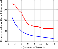
(a) bfi objective value

(b) neo objective value

(c) harman objective value

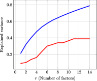
(d) bfi explained variance

(e) neo explained variance

(f) harman explained variance

Figure 5: Figure showing performance of NExOS in solving factor analysis problem for different datasets. Each column represents one dataset. The first and second row compares training loss and proportion of the variance explained of the solutions found by NExOS (shown in blue) and the nuclear norm heuristic (shown in red).

Performance measures

We consider two performance measures. First, we compare the training loss $\left\|\Sigma-X-D\right\|_{F}^{2}$ of the solutions found by NExOS and the nuclear norm heuristic. As both NExOS and the nuclear norm heuristic provide a point from the feasible set of (FA), such a comparison of training losses tells us which algorithm is providing a better quality solution. Second, we compute the proportion of explained variance, which represents how well the $r$-common factors explain the residual covariance, i.e., $\Sigma-D$. For a given $r$, input proportion of variance explained by the $r$ common factors is given by: $\sum_{i=1}^{r}\sigma_{i}(X)/\sum_{i=1}^{p}\sigma_{i}(\Sigma-D),$ where $X,D$ are inputs, that correspond to solutions found by NExOS or the nuclear norm heuristic. As $r$ increases, the explained variance increases to $1$. The higher the value of the explained variance for a certain solution, the better is the quality of the solution.

Description of the datasets

We consider three different real-world bench-mark datasets that are popularly used for factor analysis. The bfi, neo , and Harman74 datasets contain (2800 observations, 28 variables), (1000 observations, 30 variables), and (145 observations, 24 variables), respectively.

Setup

In applying NExOS for the factor analysis problem, we initialize our iterates with $Z_{0}:=\Sigma$ and $z_{0}:=\mathbf{0}$. All the other parameters are kept at their default values as stated in the beginning of §4. For each dataset, we vary the number of factors from $1$ to $\lfloor p/2\rfloor$, where $p$ is the size of the underlying matrix $\Sigma$.

Results

Figure 5 shows performance of NExOS in solving the factor analysis problem for different datasets, with each row representing one dataset. The first row compares the training loss of the solution found by NExOS and the nuclear norm heuristic. We see that for all the datasets, NExOS finds a solution with a training loss that is considerably smaller than that of the nuclear norm heuristic. The second row shows the proportion of variance explained by the algorithms considered for the datasets considered (higher is better). We see that in terms of the proportion of explained variance, NExOS delivers larger values than that of the nuclear norm heuristic for different values of $r$, which is indeed desirable. NExOS consistently provides solutions with better objective value and explained variance compared to the nuclear norm heuristic.

5 Conclusion

In this paper, we have presented NExOS, a first-order algorithm to solve optimization problems with convex cost functions over nonconvex constraint sets— a problem structure that is satisfied by a wide range of nonconvex optimization problems including sparse and low-rank optimization. We have shown that, under mild technical conditions, NExOS is able to find a locally optimal point of the original problem by solving a sequence of penalized problems with strictly decreasing penalty parameters. We have implemented our algorithm in the Julia package NExOS.jl and have extensively tested its performance on a wide variety of nonconvex optimization problems. We have demonstrated that NExOS is able to compute high quality solutions at a speed that is competitive with tailored algorithms.

Appendix A Proof and derivation to results in $\S$1

A.1 Lemma regarding prox-regularity of intersection of sets

Lemma 3.

Consider the nonempty constraint set $\mathcal{X}=\mathcal{\mathcal{C}\bigcap\mathcal{N}}\subseteq\mathbf{E}$, where $\mathcal{C}$ is compact and convex, and $\mathcal{N}$ is prox-regular at $x\in\mathcal{X}$. Then $\mathcal{X}$ is prox-regular at $x$.

Proof to Lemma 3

To prove this result we record the following result from [6], where by $d_{\mathcal{S}}(x)$ we denote the Euclidean distance of a point $x$ from the set $\mathcal{S}$, and $\overline{\mathcal{S}}$ denotes closure of a set $\mathcal{X}$.

Lemma 4 (Intersection of prox-regular sets [6, Corollary 7.3(a)]).

Let $\mathcal{S}_{1},\mathcal{S}_{2}$ be two closed sets in $\mathbf{E},$ such that $\mathcal{S}=\mathcal{S}_{1}\bigcap\mathcal{S}_{2}\neq\emptyset$ and both $\mathcal{S}_{1},\mathcal{S}_{2}$ are prox-regular at $x\in\mathcal{S}$. If $\mathcal{S}$ is metrically calm at $x$, i.e., if there exist some $\varsigma>0$ and some neighborhood of $x$ denoted by $\mathcal{B}$ such that $d_{\mathcal{S}}(y)\leq\varsigma(d_{\mathcal{S}_{1}}(y)+d_{\mathcal{S}_{2}}(y))$ for all $y\in\mathcal{B}$, then $\mathcal{S}$ is prox-regular at $x$.

Proof.

(proof to Lemma 3) By definition, projection onto $\mathcal{N}$ is single-valued on some open ball $B(x;a)$ with center $x$ and radius $a>0$ [48, Theorem 1.3]. The set $\mathcal{C}$ is compact and convex, hence projection onto $\mathcal{C}$ is single-valued around every point, hence single-valued on $B(x;a)$ as well [3, Theorem 3.14, Remark 3.15]. Note that for any $y\in B(x;a)$, $d_{\mathcal{X}}(y)=0$ if and only if both $d_{\mathcal{C}}(y)$ and $d_{\mathcal{N}}(y)$ are zero. Hence, for any $y\in B(x;a)\bigcap\mathcal{X}$, the metrically calmness condition is trivially satisfied. Next, recalling that the distance from a closed set is continuous [51, Example 9.6], over the compact set $\overline{B(x;a)\setminus\mathcal{X}}$, define the function $h$, such that $h(y)=1$ if $y\in\mathcal{X}$, and $h(y)=d_{\mathcal{X}}(y)/(d_{\mathcal{C}}(y)+d_{\mathcal{N}}(y))$ else. The function $h$ is upper-semicontinuous over $\overline{B(x;a)\setminus\mathcal{X}}$, hence it will attain a maximum $\varsigma>0$ over $\overline{B(x;a)\setminus\mathcal{X}}$ [52, Theorem 4.16], thus satisfying the metrically calmness condition on $B(x;a)\setminus\mathcal{X}$ as well. Hence, using Lemma 4, the constraint set $\mathcal{X}$ is prox-regular at $x$. ∎

A.2 Inner algorithm of NExOS from Douglas-Rachford splitting

We now discuss how to construct Algorithm 2 by applying Douglas-Rachford splitting to ($\mathcal{P}_{\mu}$). If we apply Douglas-Rachford splitting [3, page 401] to ($\mathcal{P}_{\mu}$) with penalty parameter $\mu$, we have the following variant with three sub-iterations:

$$x^{n+1} =\mathbf{prox}_{\gamma f}\left(z^{n}\right)$$ (DRS)

$$y^{n+1} =\mathbf{prox}_{\gamma\prescript{\mu}{}{\bbiota}}\left(2x^{n+1}-z^{n}\right)$$

$$z^{n+1} =z^{n}+y^{n+1}-x^{n+1}.$$

The computational cost for $\mathbf{prox}_{\gamma\prescript{\mu}{}{\bbiota}}$ is the same as computing a projection onto the constraint set $\mathcal{X}$, as we will show in Lemma 5 below.

Lemma 5 (Computing $\mathbf{prox}_{\gamma\prescript{\mu}{}{\bbiota}}(x)$ ).

Consider the nonconvex compact constraint set $\mathcal{X}$ in ($\mathcal{P}$). Denote $\kappa=1/(\beta\gamma+1)\in[0,1]$ and $\theta=\mu/(\gamma\kappa+\mu)\in[0,1]$. Then, for any $x\in\mathbf{E}$, and for any $\mu,\beta,\gamma>0$, we have $\mathbf{prox}_{\gamma\prescript{\mu}{}{\bbiota}}\left(x\right)=\theta\kappa x+\left(1-\theta\right)\mathop{{\bf\Pi}}\left(\kappa x\right)$.

Proof.

Proof follows from [5, Theorem 6.13, Theorem 6.63]. It should be noted that [5, Theorem 6.13, Theorem 6.63] assume convexity of the functions in the theorem statements, but its proof does not require convexity and works for nonconvex functions as well. ∎

Combining (DRS), [5, Theorem 6.13], and Lemma 5, we arrive at Algorithm 2.

Appendix B Proofs and derivations to the results in $\S$3

B.1 Modifying NExOS for nonsmooth and convex loss function

We now discuss how to modify NExOS when the loss function is nonsmooth and convex. The key idea is working with a strongly convex, smooth, and arbitrarily close approximation of $f$; such smoothing techniques are very common in optimization [45, 5]. The optimization problem in this case, where the positive regularization parameter is denoted by $\widetilde{\beta}$, is given by: $\min_{x}\phi(x)+(\widetilde{\beta}/2)\|x\|^{2}+\iota(x)$, where the setup is same as ($\mathcal{P}$), except the function $\phi:\mathbf{E}\to\mathbf{R}\cup\left\{+\infty\right\}$ is lower-semicontinuous, proper, and convex. Let $\beta\coloneqq\widetilde{\beta}/2$. For a $\nu$ that is arbitrarily small, define the following $\beta$ strongly convex and $(\nu^{-1}+\beta)$-smooth function: $f\coloneqq\prescript{\nu}{}{\phi}(\cdot)+(\beta/2)\|\cdot\|^{2}$ where $\prescript{\nu}{}{\phi}$ is the Moreau envelope of $\phi$ with paramter $\nu$. Following the properties of the Moreau envelope of a convex function discussed in §2, the following optimization problem acts as an arbitrarily close approximation to the first nonsmooth convex problem: $\min_{x}f+(\beta/2)\|x\|^{2}+\iota(x)$, which has the same setup as ($\mathcal{P}$). We can compute $\mathbf{prox}_{\gamma f}(x)$ using the formula in by [5, Theorem 6.13, Theorem 6.63]. Then, we apply NExOS to $\min_{x}f+(\beta/2)\|x\|^{2}+\iota(x)$ and proceed in the same manner as discussed earlier.

B.2 Proof to Proposition 1

B.2.1 Proof to Proposition 1(i)

We prove (i) in three steps. In the first step, we show that for any $\mu>0$, $f+\prescript{\mu}{}{\bbiota}$ will be differentiable on some $B(\bar{x};r_{\textrm{diff}})$ with $r_{\textrm{diff}}>0$. In the second step, we then show that, for any $\mu\in(0,1/\beta],$ $f+\prescript{\mu}{}{\bbiota}$ will be strongly convex and differentiable on some $B(\bar{x};r_{\textrm{cvxdiff}})$. In the third step, we will show that there exist $\mu_{\textrm{max}}>0$ such that for any $\mu\in(0,\mu_{\textrm{max}}]$, $f+\prescript{\mu}{}{\bbiota}$ will be strongly convex and smooth on some $B(\bar{x};r_{\textrm{max}})$ and will attain the unique local minimum $x_{\mu}$ in this ball.

Proof of the first step

To prove the first step, we start with the following lemma regarding differentiability of $\prescript{\mu}{}{\iota}$.

Lemma 6 (Differentiability of $\prescript{\mu}{}{\iota}$).

Let $\bar{x}$ be a local minimum to ($\mathcal{P}$), where Assumptions 1 and 2 hold. Then there exists some $r_{\textup{diff}}>0$ such that for any $\mu>0$: (i) the function $\prescript{\mu}{}{\iota}$ is differentiable on $B(\bar{x};r_{\textup{diff}})$ with derivative $\nabla\prescript{\mu}{}{\iota}=(1/\mu)(\mathbb{I}-\mathop{{\bf\Pi}}),$ and (ii) the projection operator $\mathop{{\bf\Pi}}$ onto $\mathcal{X}$ is single-valued and Lipschitz continuous on $B(\bar{x};r_{\textup{diff}})$.

Proof.

From [48, Theorem 1.3(e)], there exists some $r_{\textrm{diff}}>0$ such that the function $d^{2}$ is differentiable on $B(\bar{x};r_{\textrm{diff}})$. As $\prescript{\mu}{}{\iota}=(1/2\mu)d^{2}$ from (3), it follows that for any $\mu>0,$ $\prescript{\mu}{}{\iota}$ is differentiable on $B(\bar{x};r_{\textrm{diff}})$ which proves the first part of (i). The second part of (i) follows from the fact that $\nabla d^{2}(x)=2\left(x-\mathop{{\bf\Pi}}(x)\right)$ whenever $d^{2}$ is differentiable at $x$ [48, page 5240]. Finally, from [48, Lemma 3.2], whenever $d^{2}$ is differentiable at a point, projection $\mathop{{\bf\Pi}}$ is single-valued and Lipschitz continuous around that point, and this proves (ii). ∎

Due to the lemma above, $f+\prescript{\mu}{}{\bbiota}$ will be differentiable on $B(\bar{x};r_{\textrm{diff}})$ with $r_{\textrm{diff}}>0$, as $f$ and $(\beta/2)\|\cdot\|^{2}$ are differentiable. Also, due to Lemma 6(ii), projection operator $\mathop{{\bf\Pi}}$ is $\widetilde{L}$-Lipschitz continuous on $B(\bar{x};r_{\textrm{diff}})$ for some $\widetilde{L}>0$. This proves the first step.

Proof of the second step

To prove this step, we are going to record: (1) the notion of general subdifferential of a function, followed by (2) the definition of prox-regularity of a function and its connection with prox-regular set, and (3) a helper lemma regarding convexity of the Moreau envelope under prox-regularity.

Definition 3 (Fenchel, Fréchet, and general subdifferential).

For any lower-semicontinuous function $h:\mbox{{\bf R}}^{n}\to\mbox{{\bf R}}\cup\{\infty\}$, its Fenchel subdifferential $\partial h$ is defined as [22, page 1]: $u\in\partial h(x)\Leftrightarrow h(y)\geq h(x)+\left\langle u\mid y-x\right\rangle$ for all $y\in\mbox{{\bf R}}^{n}$. For the function $h$, its Fréchet subdifferential $\partial^{F}h$ (also known as regular subdifferential) at a point $x$ is defined as [22, Definition 2.5]: $u\in\partial^{F}h(x)\Leftrightarrow\liminf_{y\to 0}\,(h(x+y)-h(x)-\langle u\mid y\rangle)/\|y\|\geq 0$. Finally, the general subdifferential of $h$, denoted by $\partial^{G}h$, is defined as [50, Equation (2.8)]: $u\in\partial^{G}h(x)\Leftrightarrow u_{n}\to u,x_{n}\to x,f(x_{n})\to f(x),$ for some $(x_{n},u_{n})\in\mathop{{\bf gra}}\partial^{F}h$. If $h$ is additionally convex, then $\partial h=\partial^{F}h=\partial^{G}h$ [22, Property (2.3), Property 2.6].

Definition 4 (Connection between prox-regularity of a function and a set [47, Definition 1.1 ]).

A function $h:\mathbf{R}^{n}\to\mathbf{R}\cup\{\infty\}$ that is finite at $\tilde{x}$ is prox-regular at $\tilde{x}$ for $\tilde{\nu}$, where $\tilde{\nu}\in\partial^{G}h(\tilde{x})$, if $h$ is locally l.s.c. at $\tilde{x}$ and there exist a distance $\sigma>0$ and a parameter $\rho>0$ such that whenever $\|x^{\prime}-\tilde{x}\|<\sigma$ and $\|x-\tilde{x}\|<\sigma$ with $x^{\prime}\neq x$, $\|h(x)-h(\tilde{x})\|<\sigma$, $\|\nu-\tilde{\nu}\|<\sigma$ with $\nu\in\partial^{G}h(x)$, we have $h(x^{\prime})>h(x)+\left\langle\nu\mid x^{\prime}-x\right\rangle-(\rho/2)\|x^{\prime}-x\|^{2}$. Also, a set $\mathcal{S}$ is prox-regular at $\tilde{x}$ for $\tilde{\nu}$ if we have the indicator function $\iota_{\mathcal{S}}$ is prox-regular at $\tilde{x}$ for $\tilde{\nu}\in\partial^{G}\iota_{\mathcal{S}}(\tilde{x})$ [47, Proposition 2.11]. The set $\mathcal{S}$ is prox-regular at $\tilde{x}$ if it is prox-regular at $\tilde{x}$ for all $\tilde{\nu}\in\partial^{G}\iota_{\mathcal{S}}(\tilde{x})$ [51, page 612].

We have the following helper lemma from [47].

Lemma 7 ([47, Theorem 5.2]).

Consider a function $h$ which is lower semicontinuous at $0$ with $h(0)=0$ and there exists $\rho>0$ such that $h(x)>-(\rho/2)\|x\|^{2}$ for any $x\neq 0$. Let $h$ be prox-regular at $\tilde{x}=0$ and $\tilde{\nu}=0$ with respect to $\sigma$ and $\rho$ ($\sigma$ and $\rho$ as described in Definition 4), and let $\lambda\in(0,1/\rho).$ Then, on some neighborhood of $0$, the function

$${}^{\lambda}h+\rho/(2-2\lambda\rho)\|\cdot\|^{2}$$ (12)

is convex, where ${}^{\lambda}h$ is the Moreau envelope of $h$ with parameter $\lambda$.

Now we start proving step 2 earnestly. To prove this result, we assume $\bar{x}=0$. This does not cause any loss of generality because this is equivalent to transferring the coordinate origin to the optimal solution and prox-regularity of a set and strong convexity of a function is invariant under such a coordinate transformation.

First, note that the indicator function of our constraint closed set $\mathcal{X}$ is lower semicontinuous due to [51, Remark after Theorem 1.6, page 11], and as $\bar{x},$ the local minimizer lies in $\mathcal{X},$ we have $\iota(\bar{x})=0$. The set $\mathcal{X}$ is prox-regular at $\bar{x}$ for all $\nu\in\partial^{G}\iota(x)$ per our setup, so using Definition 4, we have $\iota$ prox-regular at $\bar{x}=0$ for $\bar{\nu}=0\in\partial^{G}\iota(\bar{x})$ (because $\bar{x}\in\mathcal{X}$, we will have $0$ as a subgradient of $\partial\iota(\bar{x})$) with respect to some distance $\sigma>0$ and parameter $\rho>0$.

Note that the indicator function satisfies $\iota(x)=c\iota(x)$ for any $c>0$ due to its definition, so $u\in\partial^{G}\iota(x)\Leftrightarrow cu\in c\partial^{G}\iota(x)=\partial(c\iota^{G}(x))=\partial\iota^{G}(x)$ [51, Equation 10(6)] In our setup, we have $\mathcal{X}$ prox-regular at $\bar{x}$. So, setting $h\coloneqq\iota,\tilde{x}\coloneqq\bar{x}=0,$ $\tilde{\nu}\coloneqq\bar{\nu}=0$, and $\nu\coloneqq u/(\beta/2\rho)$ in Definition 4, we have $\iota$ is also prox-regular at $\bar{x}=0$ for $\bar{\nu}=0$ with respect to distance $\sigma\min\{1,\beta/2\rho\}$ and parameter $\beta/2$.

Next, because the range of the indicator function is $\{0,\infty\}$, we have $\iota(x)>-(\rho/2)\|x\|^{2}$ for any $x\neq 0$. So, we have all the conditions of Theorem 7 satisfied. Hence, applying Lemma 7, we have $(1/2\mu)\left(d^{2}+\beta\mu/(2-\beta\mu)\|\cdot\|^{2}\right)$ convex and differentiable on $B\left(\bar{x};\min\left\{\sigma\min\{1,\beta/2\rho\},r_{\textrm{diff}}\right\}\right)$ for any $\mu\in(0,2/\beta)$, where $r_{\textrm{diff}}$ comes from Lemma 6. As $r_{\textrm{diff}}$ in this setup does not depend on $\mu$, the ball does not depend on $\mu$ either. Finally, note that in our exterior-point minimization function we have $\prescript{\mu}{}{\bbiota}=(1/2\mu)\left(d^{2}+\beta\mu\|\cdot\|^{2}\right)$. So if we take $\mu\leq\frac{1}{\beta}$, then we have $(\beta/2)\mu/\left(1-\mu(\beta/2)\right)\leq\beta\mu$, and on the ball $B\left(\bar{x};\min\left\{\sigma\min\{1,\beta/2\rho\},r_{\textrm{diff}}\right\}\right)$, the function $\prescript{\mu}{}{\bbiota}$ will be convex and differentiable. But $f$ is strongly-convex and smooth, so $f+\prescript{\mu}{}{\bbiota}$ will be strongly convex and differentiable on $B\left(\bar{x};\min\left\{\sigma\min\{1,\beta/2\rho\},r_{\textrm{diff}}\right\}\right)$ for $\mu\in(0,1/\beta]$. This proves step 2.

Proof of the third step

As point $\bar{x}\in\mathcal{X}$ is a local minimum of ($\mathcal{P}$), from Definition 2, there is some $r>0$ such that for all $y\in\overline{B}(\bar{x};r),$ we have $f(\bar{x})+(\beta/2)\|\bar{x}\|^{2}<f(y)+(\beta/2)\|y\|^{2}+\iota(y).$ Then, due to the first two steps, for any $\mu\in(0,1/\beta]$, the function $f+\prescript{\mu}{}{\bbiota}$ will be strongly convex and differentiable on $B\left(\bar{x};\min\left\{\sigma\min\{1,\beta/2\rho\},r_{\textrm{diff}}\right\}\right)$. For notational convenience, denote $r_{\textrm{max}}\coloneqq\min\left\{\sigma\min\{1,\beta/2\rho\},r_{\textrm{diff}}\right\},$ which is a constant. As $f+\prescript{\mu}{}{\bbiota}$ is a global underestimator of and approximates the function $f+(\beta/2)\|\cdot\|^{2}+\iota$ with arbitrary precision as $\mu\to 0$, the previous statement and [51, Theorem 1.25] imply that there exist some $0<\mu_{\textrm{max}}\leq 1/\beta$ such that for any $\mu\in(0,\mu_{\textrm{max}}],$ the function $f+\prescript{\mu}{}{\bbiota}$ will achieve a local minimum $x_{\mu}$ over $B(\bar{x};r_{\textrm{max}})$ where $\nabla(f+\prescript{\mu}{}{\bbiota})$ vanishes, i.e.,

$$\nabla(f+\prescript{\mu}{}{\bbiota})(x_{\mu}) =\text{$\nabla$}f(x_{\mu})+\beta x_{\mu}+(1/\mu)\left(x_{\mu}-\mathop{{\bf\Pi}}\left(x_{\mu}\right)\right)=0$$ (13)

$$\Rightarrow x_{\mu} =(1/(\beta\mu+1))\left(\mathop{{\bf\Pi}}(x_{\mu})-\mu\nabla f(x_{\mu})\right).$$ (14)

As the right hand side of the last equation is a singleton, this minimum must be unique. Finally to show the smoothness $f+\prescript{\mu}{}{\bbiota}$, for any $x\in B(\bar{x};r_{\textrm{max}}),$ we have

$$\nabla\left(f+\prescript{\mu}{}{\bbiota}\right)(x)\overset{a)}{=}\nabla f(x)+\left(\beta+(1/\mu)\right)x-(1/\mu)\mathop{{\bf\Pi}}(x),$$ (15)

where $a)$ uses Lemma 6. Thus, for any $x_{1},x_{2}\in B(\bar{x};r_{\textrm{max}})$ we have $\|\nabla(f+(\beta/2)\|\cdot\|^{2}+\prescript{\mu}{}{\iota})(x_{1})-\nabla(f+(\beta/2)\|\cdot\|^{2}+\prescript{\mu}{}{\iota})(x_{2})\|\leq(L+\beta+(1/\mu)+\widetilde{L})\|x_{1}-x_{2}\|$, where we have used the following: $\nabla f$ is $L$-Lipschitz everywhere due to $f$ being an $L-$smooth function in $\mathbf{E}$ ([3, Theorem 18.15]), and $\mathop{{\bf\Pi}}$ is $\widetilde{L}$-Lipschitz continuous on $B(\bar{x};r_{\textrm{max}})$, as shown in step 1. This completes the proof for (i).

(ii): Using [51, Theorem 1.25], as $\mu\to 0,$ we have $x_{\mu}\to\bar{x},\textrm{ and }\left(f+\prescript{\mu}{}{\bbiota}\right)(x_{\mu})\to f(\bar{x})+(\beta/2)\|\bar{x}\|^{2}.$ Note that $x_{\mu}$ reaches $\bar{x}$ only in limit, as otherwise Assumption 2 will be violated.

B.3 Proof to Proposition 2

B.3.1 Proof to Proposition 2(i)

We will use the following definition.

Definition 5 (Resolvent and reflected resolvent [3, pages 333, 336]).

For a lower-semicontinuous, proper, and convex function $h,$ the resolvent and reflected resolvent of its subdifferential operator are defined by $\mathbb{J}_{\gamma\partial h}=\left(\mathbb{I}+\gamma\partial h\right)^{-1}$ and $\mathbb{R}_{\gamma\partial h}=2\mathbb{J}_{\gamma\partial h}-\mathbb{I},$ respectively.

The proof of (i) is proven in two steps. First, we show that the reflection operator of $\mathbb{T}_{\mu},$ defined by

$$\mathbb{R}_{\mu}=2\mathbb{T}_{\mu}-\mathbb{I},$$ (16)

is contractive on $B(\bar{x},r_{\textrm{max}})$, and using this we show that $\mathbb{T}_{\mu}$ in also contractive there in the second step. To that goal, note that $\mathbb{R}_{\mu}$ can be represented as:

$$\mathbb{R}_{\mu}=(2\mathbf{prox}_{\gamma\prescript{\mu}{}{\bbiota}}-\mathbb{I})(2\mathbf{prox}_{\gamma f}-\mathbb{I}),$$ (17)

which can be proven by simply using (5) and (16) on the left-hand side and by expanding the factors on the right-hand side. Now, the operator $2\mathbf{prox}_{\gamma f}-\mathbb{I}$ associated with the $\alpha$-strongly convex and $L$-smooth function $f$ is a contraction mapping for any $\gamma>0$ with the contraction factor $\kappa=\max\left\{(\gamma L-1)/(\gamma L+1),(1-\gamma\alpha)/(\gamma\alpha+1)\right\}\in(0,1)$, which follows from [30, Theorem 1]. Next, we show that $2\mathbf{prox}_{\gamma\prescript{\mu}{}{\bbiota}}-\mathbb{I}$ is nonexpansive on $B(\bar{x};r_{\textup{max}})$ for any $\mu\in(0,\mu_{\textrm{max}}]$. For any $\mu\in(0,\mu_{\textrm{max}}]$, define the function $g$ as follows. We have $g(y)=\prescript{\mu}{}{\bbiota}(y)$ if $y\in B(\bar{x};r_{\textup{max}}),$$g(y)=\liminf_{\tilde{y}\to y}\prescript{\mu}{}{\bbiota}(\tilde{y})$ if $\|y-\bar{x}\|=r_{\textrm{max}}$, and $g(y)=\infty$ else. The function $g$ is lower-semicontinuous, proper, and convex everywhere due to [3, Lemma 1.31 and Corollary 9.10 ]. As a result for $\mu\in(0,\mu_{\textrm{max}}]$, we have $\mathbf{prox}_{\gamma g}=\mathbb{J}_{\gamma\partial g}$ on $\mathbf{E}$ and $\mathbf{prox}_{\gamma g}$ is firmly nonexpansive and single-valued everywhere, which follows from [3, Proposition 12.27, Proposition 16.34, and Example 23.3]. But, for $y\in B(\bar{x};r_{\textup{max}}),$ we have $\prescript{\mu}{}{\bbiota}(y)=g(y)$ and $\nabla\prescript{\mu}{}{\bbiota}(y)=\partial g(y)$. Thus, on $B(\bar{x};r_{\textup{max}}),$ the operator $\mathbf{prox}_{\gamma\prescript{\mu}{}{\bbiota}}=\mathbb{J}_{\gamma\nabla\prescript{\mu}{}{\bbiota}}$, and it is firmly nonexpansive and single-valued for $\mu\in(0,\mu_{\textrm{max}}]$. Any firmly nonexpansive operator $\mathbb{A}$ has a nonexpansive reflection operator $2\mathbb{A}-\mathbb{I}$ on its domain of firm nonexpansiveness [3, Proposition 4.2]. Hence, on $B(\bar{x};r_{\textup{max}}),$ for $\mu\in(0,\mu_{\textrm{max}}]$ the operator $2\mathbf{prox}_{\gamma\prescript{\mu}{}{\bbiota}}-\mathbb{I}$ is nonexpansive using (17).

Now we show that $\mathbb{R}_{\mu}$ is contractive for every $x_{1},x_{2}\in B(\bar{x};r_{\textup{max}})$ and $\mu\in(0,\mu_{\textrm{max}}]$, we have $\|\mathbb{R}_{\mu}(x_{1})-\mathbb{R}_{\mu}(x_{2})\|\leq\|(2\mathbf{prox}_{\gamma f}-\mathbb{I})(x_{1})-(2\mathbf{prox}_{\gamma f}-\mathbb{I})(x_{2})\|\leq\text{$\kappa$}\|x_{1}-x_{2}\|$ where the last inequality uses $\kappa$-contractiveness of $2\mathbf{prox}_{\gamma f}-\mathbb{I}$ thus proving that $\mathbb{R}_{\mu}$ acts as a contractive operator on $B(\bar{x};r_{\textup{max}})$ for $\mu\in(0,\mu_{\textrm{max}}]$. Similarly, for any $x_{1},x_{2}\in B(\bar{x};r_{\textup{max}}),$ using ($\mathcal{A}_{\mu}$) and the triangle inequality we have $\|\mathbb{T}_{\mu}(x_{1})-\mathbb{T}_{\mu}(x_{2})\|\leq(1+\kappa)/2\|x_{1}-x_{2}\|$ and as $\kappa^{\prime}=(1+\kappa)/2\in[0,1);$ the operator $\mathbb{T}_{\mu}$ is $\kappa^{\prime}-$contractive on on $B(\bar{x};r_{\textup{max}}),$ for $\mu\in(0,\mu_{\textrm{max}}]$.

B.3.2 Proof to Proposition 2(ii)

Recalling $\mathbb{T}_{\mu}=(1/2)\mathbb{R}_{\mu}+(1/2)\mathbb{I}$ from (16), using (17), and then expanding, and finally using Lemma 5 and triangle inequality, we have for any $\mu,\tilde{\mu}\in(0,\mu_{\textrm{max}}],\;x\in B(\bar{x};r_{\textup{max}}),$ and $y=2\mathbf{prox}_{\gamma f}(x)-x$:

$$\left\|\mathbb{T}_{\mu}(x)-\mathbb{T}_{\tilde{\mu}}(x)\right\| \leq\left\|\left(\mu/(\gamma+\mu(\beta\gamma+1))-\tilde{\mu}/(\gamma+\tilde{\mu}(\beta\gamma+1))\right)\right\|\left\|y\right\|$$

$$+\left\|\left(\gamma/(\gamma+\mu(\beta\gamma+1))-\gamma/(\gamma+\tilde{\mu}(\beta\gamma+1))\right)\right\|\left\|\mathop{{\bf\Pi}}\left(y/(\beta\gamma+1)\right)\right\|.$$ (18)

Now, in (18), the coefficient of $\|y\|$ satisfies $\|\mu/(\gamma+\mu(\beta\gamma+1))-\tilde{\mu}/(\gamma+\tilde{\mu}(\beta\gamma+1))\|\leq(1/\gamma)\|\mu-\tilde{\mu}\|$ and similarly the coefficient of $\|\mathop{{\bf\Pi}}\left(y/(\beta\gamma+1)\right)\|$ satisfies

$$\|\gamma/(\gamma+\mu(\beta\gamma+1))-\gamma/(\gamma+\tilde{\mu}(\beta\gamma+1))\| \leq(\beta+(1/\gamma))\|\mu-\tilde{\mu}\|.$$

Putting the last two inequalities in (18), and then replacing $y=2\mathbf{prox}_{\gamma f}(x)-x$, we have for any $x\in\mathcal{B}$, and for any $\mu,\tilde{\mu}\in\mbox{{\bf R}}_{++}$,

$$\left\|\mathbb{T}_{\mu}(x)-\mathbb{T}_{\tilde{\mu}}(x)\right\|\leq(1/\gamma)\left\|\mu-\tilde{\mu}\right\|\|y\|+\left(\beta+(1/\gamma)\right)\|\mu-\tilde{\mu}\|\left\|\mathop{{\bf\Pi}}\left(y/(\beta\gamma+1)\right)\right\|$$

$$= \{(1/\gamma)\|2\mathbf{prox}_{\gamma f}(x)-x\|+(\beta+(1/\gamma))\|\mathop{{\bf\Pi}}((2\mathbf{prox}_{\gamma f}(x)-x)/(\beta\gamma+1))\|\}\|\mu-\tilde{\mu}\|.$$ (19)

Now, as $B(\bar{x};r_{\textup{max}})$ is a bounded set and $x\in\mathcal{B}$, norm of the vector $y=2\mathbf{prox}_{\gamma f}(x)-x$ can be upper-bounded over $B(\bar{x};r_{\textup{max}})$ because $2\mathbf{prox}_{\gamma f}-\mathbb{I}$ is continuous (in fact contractive) as shown in (i). Similarly, $\|\mathop{{\bf\Pi}}\left((2\mathbf{prox}_{\gamma f}(x)-x)/(\beta\gamma+1)\right)\|$ can be upper-bounded on $B(\bar{x};r_{\textup{max}})$. Combining the last two-statements, it follows that there exists some $\ell>0$ such that

$$\sup_{x\in B(\bar{x};r_{\textup{max}})}(1/\gamma)\|2\mathbf{prox}_{\gamma f}(x)-x\|+(\beta+1/\gamma)\left\|\mathop{{\bf\Pi}}\left((2\mathbf{prox}_{\gamma f}(x)-x)/(\beta\gamma+1)\right)\right\|\leq\ell,$$

and putting the last inequality in (19), we arrive at the claim.

B.4 Proof to Proposition 3

The structure of the proof follows that of [3, Proposition 25.1(ii)]. Let $\mu\in(0,\mu_{\textrm{max}}].$ Recalling Definition 5, and due to Proposition 1(i), $x_{\mu}\in B(\bar{x};r_{\textrm{max}})$ satisfies

$$x_{\mu}=\mathop{{\rm argmin}}_{B(\bar{x};r_{\textup{max}})}f(x)+\prescript{\mu}{}{\bbiota}(x)=\mathop{{\bf zer}}(\nabla f+\nabla\prescript{\mu}{}{\bbiota})$$

$$\overset{a)}{\Leftrightarrow} \left(\exists y\in\mathbf{E}\right)\;x_{\mu}=\mathbb{J}_{\gamma\nabla\prescript{\mu}{}{\bbiota}}\mathbb{R}_{\gamma\nabla f}(y)\textrm{ and }x_{\mu}=\mathbb{J}_{\gamma\nabla f}(y),$$ (20)

where $a)$ uses the facts (shown in the proof to Proposition 2) that: (i) $\mathbb{J}_{\gamma\nabla f}$ is a single-valued operator everywhere, whereas $\mathbb{J}_{\gamma\nabla\prescript{\mu}{}{\bbiota}}$ is a single-valued operator on the region of convexity $B(\bar{x};r_{\textrm{max}})$, and (ii) $x_{\mu}=\mathbb{J}_{\gamma\nabla f}(y)$ can be expressed as $x_{\mu}=\mathbb{J}_{\gamma\nabla f}(y)\Leftrightarrow 2x_{\mu}-y=\left(2\mathbb{J}_{\gamma\nabla f}-\mathbb{I}\right)y=\mathbb{R}_{\gamma\nabla f}(y)$. Also, using the last expression, we can write the first term of (20) as $\mathbb{J}_{\gamma\nabla\prescript{\mu}{}{\bbiota}}\mathbb{R}_{\gamma\nabla f}(y)=x_{\mu}\Leftrightarrow y\in\mathop{{\bf fix}}(\mathbb{R}_{\gamma\nabla\prescript{\mu}{}{\bbiota}}\mathbb{R}_{\gamma\nabla f})$. Because for lower-semicontinuous, proper, and convex function, the resolvent of the subdifferential is equal to its proximal operator [3, Proposition 12.27, Proposition 16.34, and Example 23.3], we have $\mathbb{J}_{\gamma\partial f}=\mathbf{prox}_{\gamma f}$ with both being single-valued. Using the last fact along with (20), $y\in\mathop{{\bf fix}}(\mathbb{R}_{\gamma\nabla\prescript{\mu}{}{\bbiota}}\mathbb{R}_{\gamma\nabla f})$, we have $x_{\mu}\in\mathbf{prox}_{\gamma f}\left(\mathop{{\bf fix}}\left(\mathbb{R}_{\gamma\nabla\prescript{\mu}{}{\bbiota}}\mathbb{R}_{\gamma\partial f}\right)\right)$, but $x_{\mu}$ is unique due to Proposition 1, so the inclusion can be replaced with equality. Thus $x_{\mu}$, satisfies $x_{\mu}=\mathbf{prox}_{\gamma f}\left(\mathop{{\bf fix}}\left(\mathbb{R}_{\gamma\nabla\prescript{\mu}{}{\bbiota}}\mathbb{R}_{\gamma\partial f}\right)\right)$ where the sets are singletons due to Proposition 1 and single-valuedness of $\mathbf{prox}_{\gamma f}$. Also, because $\mathbb{T}_{\mu}$ in (5) and $\mathbb{R}_{\mu}$ in (16) have the same fixed point set (follows from (16)), using (17), we arrive at the claim.

B.5 Proof to Lemma 1

(i): This follows directly from the proof to Proposition 1.

(ii): From Lemma 1(i), and recalling that $\eta^{\prime}>1$, for any $\mu\in(0,\mu_{\textup{max}}]$, we have the first equation. Recalling Definition 5, and using the fact that for lower-semicontinuous, proper, and convex function, the resolvent of the subdifferential is equal to its proximal operator [3, Proposition 12.27, Proposition 16.34, and Example 23.3], we have $\mathbb{J}_{\gamma\partial f}=\mathbf{prox}_{\gamma f}$ with both being single-valued. So, from Proposition 3: $x_{\mu}=\mathbf{prox}_{\gamma f}(z_{\mu})=\left(\mathbb{I}+\gamma\partial f\right)^{-1}(z_{\mu})\Leftrightarrow z_{\mu}=x_{\mu}+\gamma\nabla f(x_{\mu})$. Hence, for any $\mu\in(0,\mu_{\textup{max}}]$:

$$\|z_{\mu}-\bar{x}\|=\|x_{\mu}+\gamma\nabla f(x_{\mu})-\bar{x}\|\leq\|x_{\mu}-\bar{x}\|+\gamma\|\nabla f(x_{\mu})\|$$

$$\Leftrightarrow r_{\textrm{max}}-\|z_{\mu}-\bar{x}\|\geq r_{\textrm{max}}-\|x_{\mu}-\bar{x}\|-\gamma\|\nabla f(x_{\mu})\|\overset{a)}{\geq}(\eta^{\prime}-1)r_{\textrm{max}}/\eta^{\prime}-\gamma\|\nabla f(x_{\mu})\|,$$

where $a)$ uses the first equation of Lemma 1(ii). Because, for the strongly convex and smooth function $f,$ its gradient is bounded over a bounded set $B(\bar{x};r_{\textup{max}})$ [49, Lemma 1, §1.4.2], then for $\gamma$ satisfying the fourth equation of Lemma 1(ii) and the definition of $\psi$ in the third equation of Lemma 1(ii), we have the second equation of Lemma 1(ii) for any $\mu\in(0,\mu_{\textup{max}}].$ To prove the final equation of Lemma 1(ii), note that

$$\lim_{\mu\to 0}\left(r_{\textup{max}}-\|z_{\mu}-\bar{x}\|\right)-\psi$$

$$\overset{a)}{=}\lim_{\mu\to 0}\left(r_{\textup{max}}-\|x_{\mu}+\gamma\nabla f(x_{\mu})-\bar{x}\|\right)-(\eta^{\prime}-1)r_{\textup{max}}/\eta^{\prime}+\gamma\;\textup{max}_{x\in B(\bar{x};r_{\textup{max}})}\|\nabla f(x)\|$$

$$\overset{b)}{=}\left(r_{\textup{max}}-\|\bar{x}+\gamma\nabla f(\bar{x})-\bar{x}\|\right)-(\eta^{\prime}-1)r_{\textup{max}}/\eta^{\prime}+\gamma\;\textup{max}_{x\in B(\bar{x};r_{\textup{max}})}\|\nabla f(x)\|$$

$$=(1/\eta^{\prime})r_{\textup{max}}+\gamma\left(\textup{max}_{x\in B(\bar{x};r_{\textup{max}})}\|\nabla f(x)\|-\|\nabla f(\bar{x})\|\right)>0,$$ (21)

where in $a)$ we have used $z_{\mu}=x_{\mu}+\gamma\nabla f(x_{\mu})$ and the third equation of Lemma 1(ii), in $b)$ we have used smoothness of $f$ along with Proposition 1(ii). Inequality (21) along with the second equation of Lemma 1(ii) implies the final equation of Lemma 1(ii).

B.6 Proof to Theorem 1

We use the following result from [24] in proving Theorem 1.

Theorem 3 (Convergence of local contraction mapping [24, pp. 313-314]).

Let $\mathbb{A}:\mathbf{E}\to\mathbf{E}$ be some operator. If there exist $\tilde{x}$, $\omega\in(0,1)$, and $r>0$ such that (a) $\mathbb{A}$ is $\omega$-contractive on $B(\tilde{x};r)$, i.e., for all $x_{1},x_{2}$ in $B(\tilde{x};r)$, and (b) $\|\mathbb{A}(\tilde{x})-\tilde{x}\|\leq(1-\omega)r$. Then $\mathbb{A}$ has a unique fixed point in $B(\tilde{x};r)$ and the iteration scheme $x_{n+1}=\mathbb{A}(x_{n})$ with the initialization $x_{0}:=\tilde{x}$ linearly converges to that unique fixed point.

Furthermore, recall that NExOS (Algorithm 1) can be compactly represented using ($\mathcal{A}_{\mu}$) as follows. For any $m\in\{1,2,\ldots,N\}$ (equivalently for each $\mu_{m}\in\{\mu_{1},\ldots,\mu_{N}\}$),

$$z_{\mu_{m}}^{n+1} =\mathbb{T}_{\mu_{m}}\left(z_{\mu_{m}}^{n}\right),$$ (22)

where $z_{\mu_{m}}^{0}$ is initialized at $z_{\mu_{m-1}}$. From Proposition 2, for any $\mu\in\mathfrak{M},$ the operator $\mathbb{T}_{\mu}$ is a $\kappa^{\prime}$-contraction mapping over the region of convexity $B(\bar{x};r_{\textrm{max}})$, where $\kappa^{\prime}\in(0,1)$. From Proposition 1, there will be a unique local minimum $x_{\mu}$ of ($\mathcal{P}_{\mu}$) over $B(\bar{x};r_{\textrm{max}})$. Suppose, instead of the exact fixed point $z_{\mu_{m-1}}\in\mathop{\mathop{{\bf fix}}}\mathbb{T}_{\mu_{m-1}},$ we have computed $\widetilde{z}$, which is an $\epsilon$-approximate fixed point of $\mathbb{T}_{\mu_{m-1}}$ in $B(\bar{x};r_{\textrm{max}})$, i.e., $\|\widetilde{z}-\mathbb{T}_{\mu_{m-1}}(\widetilde{z})\|\leq\epsilon$ and $\|\widetilde{z}-z_{\mu_{m-1}}\|\leq\epsilon$, where $\epsilon\in[0,\overline{\epsilon})$. Then, we have:

$$\|\mathbb{T}_{\mu_{m-1}}(\widetilde{z})-z_{\mu_{m-1}}\|=\|\mathbb{T}_{\mu_{m-1}}(\widetilde{z})-\mathbb{T}_{\mu_{m-1}}(z_{\mu_{m-1}})\|\overset{a)}{\leq}\kappa^{\prime}\underbrace{\|\widetilde{z}-z_{\mu_{m-1}}\|}_{\leq\epsilon}\leq\epsilon,$$ (23)

where $a)$ uses $\kappa^{\prime}$-contractive nature of $\mathbb{T}_{\mu_{m-1}}$ over $B(\bar{x};r_{\textrm{max}})$. Hence, using triangle inequality,

$$\|\widetilde{z}-\bar{x}\|\overset{a)}{\leq}\|\widetilde{z}-\mathbb{T}_{\mu_{m-1}}(\widetilde{z})\|+\|\mathbb{T}_{\mu_{m-1}}(\widetilde{z})-z_{\mu_{m-1}}\|+\|z_{\mu_{m-1}}-\bar{x}\|\overset{b)}{\leq}2\epsilon+\|z_{\mu_{m-1}}-\bar{x}\|,$$

where $a)$ uses triangle inequality and $b)$ uses (23). As $\epsilon\in[0,\overline{\epsilon}),$ where $\overline{\epsilon}$ is defined in (6), due to the second equation of Lemma 1(ii), we have $r_{\textrm{max}}-\|\widetilde{z}-\bar{x}\|>\psi$.

Define $\Delta=\left((1-\kappa^{\prime})\psi-\epsilon\right)/\ell,$ which will be positive due to $\epsilon\in[0,\overline{\epsilon})$ and (6). Next, select $\theta\in(0,1)$ such that $\overline{\Delta}=\theta\Delta<\mu_{1},$ hence there exists a $\rho\in(0,1)$ such that $\overline{\Delta}=(1-\rho)\mu_{1}.$ Now reduce the penalty parameter using

$${\mu}_{m}=\mu_{m-1}-\rho^{m-2}\overline{\Delta}=\rho\mu_{m-1}=\rho^{m-1}\mu_{1}$$ (24)

for any $m\geq 2$. Next, we initialize the iteration scheme $z_{\mu_{m}}^{n+1}=\mathbb{T}_{\mu_{m}}\left(z_{\mu_{m}}^{n}\right)$ at $z_{\mu_{m}}^{0}\coloneqq\widetilde{z}.$ Around this initial point, let us consider the open ball $B(\widetilde{z},\psi)$. For any $x\in B(\widetilde{z};\psi)$, we have $\|x-\bar{x}\|\leq\|x-\widetilde{z}\|+\|\widetilde{z}-\bar{x}\|<\psi+\|\widetilde{z}-\bar{x}\|<r_{\textrm{max}},$ where the last inequality follows from $r_{\textrm{max}}-\|\widetilde{z}-\bar{x}\|>\psi$. Thus we have shown that $B(\widetilde{z};\psi)\subseteq B(\bar{x};r_{\textrm{max}})$. Hence, from Proposition 2, on $B(\widetilde{z};\psi)$, the Douglas-Rachford operator $\mathbb{T}_{\mu_{m}}$ is contractive. Next, we have $\|\mathbb{T}_{\mu_{m}}(\widetilde{z})-\widetilde{z}\|\leq(1-\kappa^{\prime})\psi$, because $\|\mathbb{T}_{\mu_{m}}(\widetilde{z})-\widetilde{z}\|\overset{a)}{\leq}\|\mathbb{T}_{\mu_{m}}(\widetilde{z})-\mathbb{T}_{\mu_{m-1}}(\widetilde{z})\|+\|\mathbb{T}_{\mu_{m-1}}(\widetilde{z})-\widetilde{z}\|\overset{b)}{\leq}\ell\|\mu_{m}-\mu_{m-1}\|+\epsilon\overset{c)}{\leq}\epsilon+\ell\Delta\overset{d)}{\leq}(1-\kappa^{\prime})\psi,$ where $a)$ triangle inequality, $b)$ uses Proposition 2(ii) and $\|\widetilde{z}-\mathbb{T}_{\mu_{m-1}}(\widetilde{z})\|\leq\epsilon$, $c)$ uses (24) and  $\|\mu_{m}-\mu_{m-1}\|\leq\overline{\Delta}\leq\Delta$ $d)$ uses the definition of $\Delta$. Thus, both conditions of Theorem 3 are satisfied, and $z_{\mu_{m}}^{n}$ in (22) will linearly converge to the unique fixed point $z_{\mu_{m}}$of the operator $\mathbb{T}_{\mu_{m}}$, and $x_{\mu_{m}}^{n},\text{$y_{\mu_{m}}^{n}$}$ will linearly converge to $x_{\mu_{m}}$. This completes the proof.

B.7 Proof to Lemma 2

First, we show that, for the given initialization of $z_{\textrm{init}}$, the iterates $z_{\mu_{1}}^{n}$ stay in $\overline{B}(z_{\mu_{1}};\|z_{\textrm{init}}-z_{\mu_{1}}\|)$ for any $n\in\mbox{{\bf N}}$ via induction. The base case is true via given. Let, $z_{\mu_{1}}^{n}\in\overline{B}(z_{\mu_{1}};\|z_{\textrm{init}}-z_{\mu_{1}}\|)$. Then, $\|z_{\mu_{1}}^{n+1}-z_{\mu_{1}}\|\overset{a)}{=}\|\mathbb{T}_{\mu_{1}}(z_{\mu_{1}}^{n})-\mathbb{T}_{\mu_{1}}(z_{\mu_{1}})\|\overset{b)}{\leq}\kappa^{\prime}\|z_{\mu_{1}}^{n}-z_{\mu_{1}}\|\overset{c)}{\leq}\kappa^{\prime}\|z_{\textrm{init}}-z_{\mu_{1}}\|$, where $a)$ uses $z_{\mu_{1}}\in\mathop{\mathop{{\bf fix}}}\mathbb{T}_{\mu},$ and $b)$ uses Proposition 2, and $c)$ uses $\|z_{\mu_{1}}^{n}-z_{\mu_{1}}\|\leq\|z_{\textrm{init}}-z_{\mu_{1}}\|$. So, the iterates $z_{\mu_{1}}^{n}$ stay in $\overline{B}(z_{\mu_{1}};\|z_{\textrm{init}}-z_{\mu_{1}}\|)$. As, $\kappa^{\prime}\in(0,1)$, this inequality also implies that $z_{\mu}^{n}$ linearly converges to $z_{\mu}$ with the rate of at least $\kappa^{\prime}$. Then using similar reasoning presented in the proof to Theorem 1, we have $x_{\mu}^{n}$ and $y_{\mu}^{n}$ linearly converge to the unique local minimum $x_{\mu}$ of ($\mathcal{P}_{\mu}$). This completes the proof.

B.8 Proof to Theorem 2

The proof is based on the results in [41, Theorem 4] and [60, Theorem 4.3]. The function $f$ is $L$-Lipschitz continuous and strongly smooth, hence $f$ is a coercive function satisfying $\liminf_{\|x\|\to\infty}f(x)=\infty$ and is bounded below [3, Corollary 11.17]. Also, $\prescript{\mu}{}{\bbiota}(x)$ is jointly continuous hence lower-semicontinuous in $x$ and $\mu$ and is bounded below by definition. Let the proximal parameter $\gamma$ be smaller than or equal to $1/L$. Then due to [41, (14), (15) and Theorem 4], $\{x_{\mu}^{n},y_{\mu}^{n},z_{\mu}^{n}\}$ (iterates of the inner algorithm of NExOS for any penalty parameter $\mu$) will be bounded. This boundedness implies the existence of a cluster point of the sequence, which allows us to use [41, Theorem 4 and Theorem 1] to show that for any $z_{\textrm{init}}$, the iterates $x_{\mu}^{n}$ and $y_{\mu}^{n}$ subsequentially converges to a first-order stationary point $x_{\mu}$ satisfying $\nabla\left(f+\prescript{\mu}{}{\bbiota}\right)(x_{\mu})=0$. The rate $\min_{n\leq k}\|\nabla\left(f+\prescript{\mu}{}{\bbiota}\right)(x_{\rho\mu}^{n})\|\leq((1-\gamma L)/2L)o(1/\sqrt{k})$ is a direct application of [60, Theorem 4.3] as our setup satisfies all the conditions to apply it.

References

- [1] Alfred Auslender. Stability in mathematical programming with nondifferentiable data. SIAM Journal on Control and Optimization, 22(2):239–254, 1984.
- [2] Francis Bach. Sharp analysis of low-rank kernel matrix approximations. In Journal of Machine Learning Research, 2013.
- [3] Heinz H Bauschke and Patrick L Combettes. Convex analysis and monotone operator theory in Hilbert spaces, volume 408. Springer, 2017.
- [4] Heinz H Bauschke, Manish Krishan Lal, and Xianfu Wang. Projections onto hyperbolas or bilinear constraint sets in hilbert spaces. Journal of Global Optimization, pages 1–12, 2022.
- [5] Amir Beck. First-Order Methods in Optimization, volume 25. SIAM, 2017.
- [6] Frédéric Bernard, Lionel Thibault, and Nadia Zlateva. Prox-regular sets and epigraphs in uniformly convex Banach spaces: various regularities and other properties. Transactions of the American Mathematical Society, 363(4):2211–2247, 2011.
- [7] Dimitris Bertsimas, Martin S Copenhaver, and Rahul Mazumder. Certifiably optimal low rank factor analysis. The Journal of Machine Learning Research, 18(1):907–959, 2017.
- [8] Dimitris Bertsimas, Ryan Cory-Wright, and Jean Pauphilet. Mixed-projection conic optimization: A new paradigm for modeling rank constraints. Operations Research (accepted), 2020.
- [9] Dimitris Bertsimas, Vassilis Digalakis Jr, Michael Linghzi Li, and Omar Skali Lami. Slowly varying regression under sparsity. arXiv preprint arXiv:2102.10773, 2021.
- [10] Dimitris Bertsimas and Jack Dunn. Machine Learning Under a Modern Optimization Lens. Dynamic Ideas, MA, 2019.
- [11] Dimitris Bertsimas, Angela King, and Rahul Mazumder. Best subset selection via a modern optimization lens. The annals of statistics, pages 813–852, 2016.
- [12] Dimitris Bertsimas and Bart Van Parys. Sparse hierarchical regression with polynomials. Machine Learning, 2020.
- [13] Dimitris Bertsimas, Bart Van Parys, et al. Sparse high-dimensional regression: Exact scalable algorithms and phase transitions. The Annals of Statistics, 48(1):300–323, 2020.
- [14] Jeffrey D Blanchard, Jared Tanner, and Ke Wei. CGIHT: conjugate gradient iterative hard thresholding for compressed sensing and matrix completion. Information and Inference: A Journal of the IMA, 4(4):289–327, 2015.
- [15] Thomas Blumensath and Mike E Davies. Iterative thresholding for sparse approximations. Journal of Fourier analysis and Applications, 14(5-6):629–654, 2008.
- [16] Thomas Blumensath and Mike E Davies. Normalized iterative hard thresholding: Guaranteed stability and performance. IEEE Journal of selected topics in signal processing, 4(2):298–309, 2010.
- [17] Stephen Boyd, Neal Parikh, Eric Chu, Borja Peleato, and Jonathan Eckstein. Distributed optimization and statistical learning via the alternating direction method of multipliers. Foundations and Trends® in Machine learning, 3(1):1–122, 2011.
- [18] Stephen Boyd and Lieven Vandenberghe. Convex Optimization. Cambridge University Press, 2004.
- [19] Emmanuel Candès and Benjamin Recht. Exact matrix completion via convex optimization. Foundations of Computational Mathematics, 2009.
- [20] Emmanuel Candès, Michael B Wakin, and Stephen Boyd. Enhancing sparsity by reweighted l1 minimization. Journal of Fourier Analysis and Applications, 2008.
- [21] Francis H Clarke, Ronald J Stern, and Peter R Wolenski. Proximal smoothness and the lower- property. Journal of Convex Analysis, 2(1-2):117–144, 1995.
- [22] Rafael Correa, Alejandro Jofre, and Lionel Thibault. Characterization of lower semicontinuous convex functions. Proceedings of the American Mathematical Society, pages 67–72, 1992.
- [23] Steven Diamond, Reza Takapoui, and Stephen Boyd. A general system for heuristic minimization of convex functions over non-convex sets. Optimization Methods and Software, 33(1):165–193, 2018.
- [24] Asen L Dontchev and Ralph T Rockafellar. Implicit functions and solution mappings, volume 543. Springer, 2009.
- [25] Iain Dunning, Joey Huchette, and Miles Lubin. JuMP: A modeling language for mathematical optimization. SIAM Review, 59(2):295–320, 2017.
- [26] Maryam Fazel, Emmanuel Candès, Benjamin Recht, and Pablo Parrilo. Compressed sensing and robust recovery of low rank matrices. In Conference Record - Asilomar Conference on Signals, Systems and Computers, 2008.
- [27] Anthony V Fiacco and Garth P McCormick. Nonlinear programming: sequential unconstrained minimization techniques. SIAM, 1990.
- [28] Simon Foucart. Hard thresholding pursuit: an algorithm for compressive sensing. SIAM Journal on numerical analysis, 49(6):2543–2563, 2011.
- [29] Jerome Friedman, Trevor Hastie, Rob Tibshirani, et al. glmnet: Lasso and elastic-net regularized generalized linear models. R package version, 1(4):1–24, 2009.
- [30] Pontus Giselsson and Stephen Boyd. Linear convergence and metric selection for Douglas-Rachford splitting and ADMM. IEEE Transactions on Automatic Control, 62(2):532–544, Feb 2017.
- [31] Ian Goodfellow, Yoshua Bengio, and Aaron Courville. Deep Learning. MIT Press, 2016. http://www.deeplearningbook.org.
- [32] Aubrey Gress and Ian Davidson. A flexible framework for projecting heterogeneous data. In CIKM 2014 - Proceedings of the 2014 ACM International Conference on Information and Knowledge Management, 2014.
- [33] Moritz Hardt, Raghu Meka, Prasad Raghavendra, and Benjamin Weitz. Computational limits for Matrix Completion. In Journal of Machine Learning Research, 2014.
- [34] Trevor Hastie, Robert Tibshirani, and Jerome Friedman. The Elements of Statistical Learning. Springer Series in Statistics. Springer New York Inc., New York, NY, USA, 2001.
- [35] Trevor Hastie, Robert Tibshirani, and Ryan J Tibshirani. Extended comparisons of best subset selection, forward stepwise selection, and the lasso. arXiv preprint arXiv:1707.08692, 2017.
- [36] Trevor Hastie, Robert Tibshirani, and Martin Wainwright. Statistical learning with sparsity: The lasso and generalizations. Taylor & Francis, 2015.
- [37] Hussein Hazimeh and Rahul Mazumder. Fast best subset selection: Coordinate descent and local combinatorial optimization algorithms. Operations Research, 68(5):1517–1537, 2020.
- [38] Prateek Jain and Purushottam Kar. Non-convex optimization for machine learning. Foundations and Trends® in Machine Learning, 10(3-4):142–336, 2017.
- [39] Kwang-Sung Jun, Rebecca Willett, Stephen Wright, and Robert Nowak. Bilinear bandits with low-rank structure. In International Conference on Machine Learning, pages 3163–3172. PMLR, 2019.
- [40] Joonseok Lee, Seungyeon Kim, Guy Lebanon, Yoram Singer, and Samy Bengio. LLORMA: Local low-rank matrix approximation. The Journal of Machine Learning Research, 17(1):442–465, 2016.
- [41] Guoyin Li and Ting Kei Pong. Douglas–rachford splitting for nonconvex optimization with application to nonconvex feasibility problems. Mathematical programming, 159(1):371–401, 2016.
- [42] D. Russell Luke. Prox-regularity of rank constraint sets and implications for algorithms. Journal of Mathematical Imaging and Vision, 47(3):231–238, Nov 2013.
- [43] Rahul Mazumder, Trevor Hastie, and Robert Tibshirani. Spectral regularization algorithms for learning large incomplete matrices. Journal of Machine Learning Research, 2010.
- [44] Tomas Mikolov, Ilya Sutskever, Kai Chen, Greg Corrado, and Jeffrey Dean. Distributed representations of words and phrases and their compositionality. In Advances in Neural Information Processing Systems, 2013.
- [45] Yu Nesterov. Smooth minimization of non-smooth functions. Mathematical programming, 103(1):127–152, 2005.
- [46] Neal Parikh and Stephen Boyd. Proximal algorithms. Foundations and Trends® in Optimization, 1(3):127–239, 2014.
- [47] René Poliquin and R Rockafellar. Prox-regular functions in variational analysis. Transactions of the American Mathematical Society, 348(5):1805–1838, 1996.
- [48] René Poliquin, Ralph T Rockafellar, and Lionel Thibault. Local differentiability of distance functions. Transactions of the American Mathematical Society, 352(11):5231–5249, 2000.
- [49] Boris T Polyak. Introduction to optimization. Translations series in mathematics and engineering. Optimization Software, 1987.
- [50] Ralph T Rockafellar. Characterizing firm nonexpansiveness of prox mappings both locally and globally. Journal of Nonlinear and convex Analysis, 22(5), 2021.
- [51] Ralph T Rockafellar and Roger J-B Wets. Variational analysis, volume 317. Springer Science & Business Media, 2009.
- [52] Walter Rudin. Principles of Mathematical Analysis. McGraw-hill New York, 1986.
- [53] James Saunderson, Venkat Chandrasekaran, Pablo Parrilo, and Alan S Willsky. Diagonal and low-rank matrix decompositions, correlation matrices, and ellipsoid fitting. SIAM Journal on Matrix Analysis and Applications, 33(4):1395–1416, 2012.
- [54] Alexander Shapiro. Existence and differentiability of metric projections in Hilbert spaces. SIAM Journal on Optimization, 4(1):130–141, 1994.
- [55] Vivek Srikumar and Christopher D Manning. Learning distributed representations for structured output prediction. In Advances in Neural Information Processing Systems, 2014.
- [56] Lorenzo Stella, Niccolo Antonello, and Mattias Falt. ProximalOperators. jl, 2020.
- [57] Reza Takapoui. The Alternating Direction Method of Multipliers for Mixed-integer Optimization Applications. PhD thesis, Stanford University, 2017.
- [58] Reza Takapoui, Nicholas Moehle, Stephen Boyd, and Alberto Bemporad. A simple effective heuristic for embedded mixed-integer quadratic programming. International Journal of Control, pages 1–11, 2017.
- [59] Jos MF ten Berge. Some recent developments in factor analysis and the search for proper communalities. In Advances in data science and classification, pages 325–334. Springer, 1998.
- [60] Andreas Themelis and Panagiotis Patrinos. Douglas-Rachford splitting and ADMM for nonconvex optimization: Tight convergence results. SIAM Journal on Optimization, 30(1):149–181, 2020.
- [61] Andreas M Tillmann, Daniel Bienstock, Andrea Lodi, and Alexandra Schwartz. Cardinality minimization, constraints, and regularization: A survey. arXiv preprint arXiv:2106.09606, 2021.
- [62] Joel A. Tropp. Just relax: Convex programming methods for identifying sparse signals in noise. IEEE Transactions on Information Theory, 2006.
- [63] M. Udell, C. Horn, R. Zadeh, and S. Boyd. Generalized low rank models. Foundations and Trends in Machine Learning, 9(1), 2016.
- [64] Jean-Philippe Vial. Strong and weak convexity of sets and functions. Mathematics of Operations Research, 8(2):231–259, 1983.