Idealised Turbulent Wake With Steady, Non-Uniform Ambient Density Stratification

Abstract

Density stratification in geophysical environments can be non-uniform in the vertical direction, particularly in thermohaline staircases and atmospheric layer transitions. Non-uniform stratification, however, is often approximated by the average ambient density change with height. This approximation is frequently made in numerical simulations because it greatly simplifies the calculations. In this paper, direct numerical simulations using $4096\times 2048\times 2048$ grid points to resolve an idealised turbulent wake in a non-uniformly stratified fluid are analysed to understand the consequences of assuming linear stratification. For flows with the same average change in density with height, but varied local stratification $d\overline{\rho}(z)/dz$, flow dynamics are dependent on the ratio $\xi=\delta_{\cal U}/\delta_{\rho}$, where $\delta_{\cal U}$ and $\delta_{\rho}$ are characteristic velocity and density vertical scale heights of the mean flow. Results suggest that a stably stratified flow will demonstrate characteristics similar to nonstratified flow when $\xi>2$, even though the average stratification is quite strong. In particular, the results show that mixing is enhanced when $\xi>2$.

1 Introduction

Geophysical flows can often be considered to have an ambient density that varies with height and to be invariant on the time scales of turbulent motion. Denoting by $\overline{\rho}(z)$ the time-independent ambient density at vertical position $z$, we define the “stratification” as $d\overline{\rho}(z)/dz$. Our interest is in the stabilising stratification that occurs in much of the ocean and atmosphere since understanding and modelling its effects on turbulence are important to predicting weather and climate and the related turbulent transport of heat, momentum and species. In particular, we focus on the dynamics of turbulence when the stratification is not uniform and on the modelling biases that may occur if a non-uniformly stratified flow is modelled as if it were uniformly stratified, that is, as if $d\overline{\rho}(z)/dz$ were a constant.

Numerous investigations have been performed concerning flow in density stratified fluids. Laboratory studies include flows of turbulent wakes (e.g., Chomaz et al., 1993; Spedding et al., 1996; Spedding, 2002; Bonnier & Eiff, 2002), grid generated turbulence (e.g., Liu, 1995; Fincham et al., 1996; Praud et al., 2005), and dynamics of monopoles and dipoles (e.g., Billant & Chomaz, 2000a; Beckers et al., 2001, 2002). Also, several numerical studies have been performed to investigate how density-stratified fluids behave; examples include horizontal layer decoupling (Herring & Métais, 1989; Métais & Herring, 1989; Waite & Bartello, 2004), turbulent mixing (Winters & D’Asaro, 1996; Staquet, 2000; Gargett et al., 2003; Peltier & Caulfield, 2003), turbulence parameterisation (Smyth & Moum, 2000b; Shih et al., 2005; Hebert & de Bruyn Kops, 2006), and flow energetics (Ivey & Imberger, 1991; Lindborg, 2006; Almalkie & de Bruyn Kops, 2012; Maffioli & Davidson, 2016; de Bruyn Kops & Riley, 2019; Portwood et al., 2019).

In the studies of density-stratified flows, such as those just cited, the assumption that the stratification is uniform and not a function of height is commonly made. However, in natural settings such as the atmosphere (Gossard et al., 1985; Dalaudier et al., 1994; Muschinski & Wode, 1998) and the ocean (Williams, 1974; Molcard & Tait, 1977; Lambert & Sturges, 1977; Schmitt et al., 1987; Boyd, 1989), density layers or “staircases” can form in which areas of well-mixed fluid are separated by thin, high density-gradient interface regions. Assuming an average density stratification $\Delta\overline{\rho}/\Delta z=(\overline{\rho}_{top}-\overline{\rho}_{bottom})/(z_{top}-z_{bottom})$ in these regions neglects the effect of local stratification differences. In figure 1 is a sketch showing layers with values of the dimensional buoyancy frequency $N$ and its spatial average $\overline{N}$ versus elevations $z$ typical of a thermohaline staircase in the ocean in which the interface stratification can be 40 to 100 times larger than the layer stratification (Gregg & Sanford, 1987).

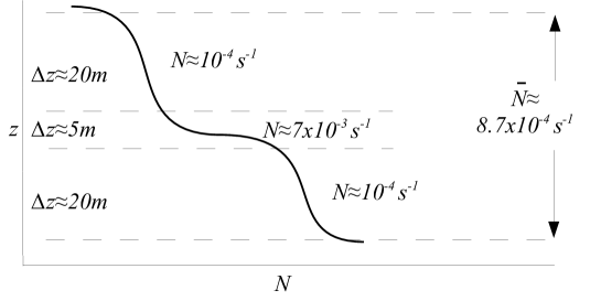
Figure 1: Cartoon of a density staircase showing two hypothetical layers subjected to moderate stratification separated by an interface of strongly stratified fluid. The numerical values are from Gregg & Sanford (1987).

Previous studies have been performed to investigate shear flow in which the initial vertical velocity and density profiles vary with height. For example, Smyth et al. (2005) investigate the ratio of turbulent diffusivities, Smyth et al. (2001) investigate a mixing efficiency defined as the ratio of Ozmidov to Thorpe length scales, Smyth & Moum (2000b, a) investigate the length scales of turbulence in a shear flow, and D’Asaro et al. (2004) investigate mixing estimates using Lagrangian tracers. In each of these studies the initial density (and velocity) profiles are a function of vertical position and change as the simulation evolves. An important difference between those studies and the current research is that here the ambient vertical density profile, $\overline{\rho}(z)$, (and hence the density stratification) is constant in time, thereby modelling a persistent, steady state thermohaline staircase or atmospheric transition layer.

The objective of this study is to investigate the effect of non-uniform density stratification on a highly idealised late wake. In particular, the wake has no source of energy so the flow is decaying. The wake has zero mean velocity, similar to that generated by a self-propelled object (although Meunier & Spedding (2006) note that it is very difficult to obtain a truly momentumless wake in a stratified fluid). The behaviour of the simulated flow is investigated for a range of stratification profiles superimposed on the same initial velocity field. The methodology and simulations are described in §2 followed by a detailed discussion of the dynamics of the simulated flow in §3, 4, and 5. Modelling implications and conclusions are presented in §6.

2 Methodology

2.1 Simulation Overview

High resolution direct numerical simulations (DNS’s) of a perturbed von Kármán vortex street are conducted. The initial conditions consist of three vortex pairs and low-level noise. There is no ambient shear and the the ambient stratification is a function of height and held constant in time. Each vortex is initialised with the following velocity profile (c.f. de Bruyn Kops et al., 2003):

$${\bf\widetilde{V}_{\theta}}={\cal\widetilde{{\cal U}}}\frac{\tilde{r}}{\tilde{r}_{m}}\exp\left[\frac{1}{2}\left(1-\left(\frac{\tilde{r}}{\tilde{r}_{m}}\right)^{2}\right)\right]\mathrm{sech}^{2}\left(\frac{\tilde{z}}{\tilde{\delta}_{\cal U}}\right)\ ,$$ (1)

where ${\cal\widetilde{{\cal U}}}$ is the initial velocity scale, $\tilde{r}_{m}$ is a radial length scale, $\tilde{\delta}_{\cal U}$ is the velocity scale height, $\tilde{r}=\sqrt{\tilde{x}^{2}+\tilde{y}^{2}}$ is the radial position, and $\tilde{z}$ is the vertical position. The convention of denoting dimensional quantities by $(\tilde{\cdot})$ is used in this section. The separation distances between vortex centres in the $\tilde{x}$ and $\tilde{y}$ directions are $\tilde{s}_{x}=2\tilde{r}_{m}$ and $\tilde{s}_{y}=1.5\tilde{r}_{m}$. In creating the initial flow condition, noise is applied to $\tilde{r}_{m}$, $\tilde{\delta}_{\cal U}$, $\tilde{s}_{x}$, $\tilde{s}_{y}$; each is randomly perturbed up to 5% of its nominal value. For example, the vertical scale for each vortex is calculated as $\tilde{\delta}_{\cal U}+0.05\lambda\tilde{\delta}_{\cal U}$, and the $y$ positions for the positive vortices are calculated as $\tilde{L}_{y}/2+\tilde{s}_{y}/2+0.05\lambda\tilde{s}_{y}$, where $\lambda$ is a [-1 1] uniformly distributed random number and $\tilde{L}_{y}$ is the span-wise ($y$) domain width.

The ambient density, $\tilde{\overline{\rho}}(\tilde{z})$, is imposed with a hyperbolic tangent vertical profile,

$$\tilde{\overline{\rho}}(\tilde{z})=\frac{\Delta\tilde{\overline{\rho}}}{2}\mathrm{tanh}\left(\frac{-\tilde{z}}{\tilde{\delta}_{\rho}}\right)\ ,$$ (2)

from which the density stratification, $d\tilde{\overline{\rho}}(\tilde{z})/d\tilde{z}$, is obtained:

$$\frac{d\tilde{\overline{\rho}}(\tilde{z})}{d\tilde{z}}=-\frac{1}{2}\frac{\Delta\tilde{\overline{\rho}}}{\tilde{\delta}_{\rho}}\mathrm{sech}^{2}\left(\frac{-\tilde{z}}{\tilde{\delta}_{\rho}}\right)\,.$$ (3)

Here $\Delta\tilde{\overline{\rho}}=\tilde{\overline{\rho}}_{top}-\tilde{\overline{\rho}}_{bottom}$ is the difference in density between the top and bottom of the numerical domain, $\tilde{z}$ is the vertical position, and $\tilde{\delta}_{\rho}$ is a characteristic height of the density profile. The vertical profiles of both the velocity (1) and density stratification (3) are $\mathrm{sech}^{2}$ with scale heights $\tilde{\delta}_{\cal U}$ and $\tilde{\delta}_{\rho}$, respectively. The parameter $\xi$ is now defined which describes the ratio of the momentum vertical length scale, $\tilde{\delta}_{\cal U}$, to the stratification vertical length scale, $\tilde{\delta}_{\rho}$, as

$$\xi\equiv\frac{\tilde{\delta}_{\cal U}}{\tilde{\delta}_{\rho}}.$$ (4)

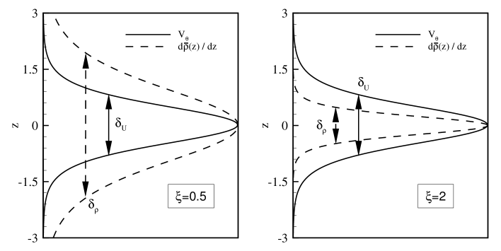
Figure 2: Velocity profile (solid) and density stratification (dashed) for $\xi=0.5$ and $\xi=2$.

Velocity and density profiles corresponding to several values of $\xi$ are shown in figure 2.

The velocity scale height is the same in all simulations; only $\tilde{\delta}_{\rho}$ is varied to obtain different values of $\xi$. The vertical profiles of $\overline{\rho}(z)$ and $d\overline{\rho}(z)/dz$ for each $\xi$ are shown in figure 3. Note that while locally $d\overline{\rho}(z)/dz$ differs for each $\xi$, the average change in density with height is the same.

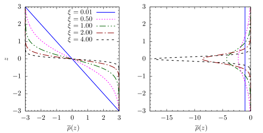
Figure 3: Ambient (nondimensional) density profile and stratification profile for several different $\xi$ (see (4)). Note $\Delta\overline{\rho}/\Delta z=-1$ for each $\xi$, but locally $d\overline{\rho}(z)/dz$ is different.

2.2 Governing Equations

The simulated flow fields satisfy the Navier-Stokes equations subject to the non-hydrostatic Boussinesq approximation. Taking $\widetilde{{\cal U}}$ as the velocity scale, $\tilde{r}_{m}$ as the length scale, $\tilde{r}_{m}|\Delta\tilde{\overline{\rho}}/\Delta\tilde{z}|$ as the density scale, $\tilde{r}_{m}/\widetilde{{\cal U}}$ as a time scale, and $\tilde{\rho}_{0}\widetilde{{\cal U}}^{2}$ as a pressure scale (where $\tilde{\rho}_{0}$ is the reference density value), the nondimensional governing equations in a non-rotating frame of reference are:

$$\nabla\cdot{\bf v}=0$$ (5a)

$$\frac{\partial{\bf v}}{\partial t}+{\bf v}\cdot\nabla{\bf v}=-\left(\frac{2\pi}{\overline{\mathrm{Fr}}}\right)^{2}\rho{\bf e}_{z}-\nabla p+\frac{1}{{Re_{r}}}\nabla^{2}{\bf v}$$ (5b)

$$\frac{\partial\rho}{\partial t}+{\bf v}\cdot\nabla\rho+w\frac{d\overline{\rho}(z)}{dz}=\frac{1}{{Re_{r}}\mathrm{Sc}}\nabla^{2}\rho$$ (5c)

where ${\bf v}=(u,v,w)$ is the velocity vector, $\rho$ and $p$ are the density and pressure deviations from their ambient values, and ${\bf e}_{z}$ is a unit vector in the vertical direction. The Reynolds, Froude, and Schmidt numbers are defined as:

$${Re_{r}} =\frac{\widetilde{{\cal U}}\tilde{r}_{m}}{\tilde{\nu}} \overline{\mathrm{Fr}} =\frac{2\pi\widetilde{{\cal U}}}{\widetilde{\overline{\mathit{N}}}\tilde{r}_{m}} \mathrm{Sc} =\frac{\tilde{\nu}}{\widetilde{{\cal D}}},$$ (6)

where $\widetilde{\overline{\mathit{N}}}^{2}=-\tilde{g}/\tilde{\rho}_{0}(\Delta\tilde{\overline{\rho}}/\Delta\tilde{z})$ is the average buoyancy frequency, and ${\cal\widetilde{{\cal D}}}$ is an effective mass diffusivity that represents the effects of salt diffusivity (ocean) or water vapour diffusivity (atmosphere) and thermal diffusivity.

All simulations are conducted using a pseudo-spectral technique by which spatial derivatives are computed using spectral methods. Time advancement is performed using a third-order Adams-Bashforth scheme with pressure projection. A spherical wave-number truncation of approximately 15/16 $\kappa_{max}$, with $\kappa_{max}$ the maximum wave number in the discrete Fourier transforms, is used to eliminate aliasing errors from wave numbers that are not already affected by truncation error. The extent of truncation error in high-resolution DNS can be understood from the cusp in the spectra in, e.g., figure 5 in Kaneda et al. (2003), which is explained in Jang & de Bruyn Kops (2007, §5). The momentum equation is advanced in time with the nonlinear term computed in vorticity form. As suggested by Kerr (1985), an alternating time-step scheme is employed for the density field to approximate the skew-symmetric form of the non-linear term, thereby minimising aliasing errors (Boyd, 2001).

Periodic boundary conditions are imposed in all directions for the simulations. This can be done because the stratification is very close to periodic in the vertical direction. To be precise, the stratification in the simulations is not exactly $\mathrm{sech}^{2}$ but rather a Fourier series approximation to it. Since the governing equations include density stratification $d\tilde{\overline{\rho}}(\tilde{z})/d\tilde{z}$, and not $\tilde{\overline{\rho}}(\tilde{z})$, periodic boundary conditions can be used.

The only difference in the parameters of each simulation is the stratification profile; $\delta_{\rho}$ is chosen so that $0.01\leq\xi\leq 4$. In other words, the velocity vertical length scale ranges from 100 times smaller to 4 times greater than the density vertical length scale (see figure 3). Values of $\delta_{\rho}$ and $\delta_{\cal U}$ for each simulation are summarised in Table 1. The case of $\xi=0.01$ is so close to being linearly stratified over the range of $z$ in the simulations that a separate linearly stratified case is not considered. The unstratified case is also considered for comparison since, when $\xi\gg 1$, much of the flow is subjected to very mild stratification.

$\xi$	0.01	0.5	1	2	4	NoStrat
$\delta_{\rho}$	69.4	1.39	0.694	0.347	0.174	N/A
$\delta_{\cal U}$	0.694	0.694	0.694	0.694	0.694	0.694

Table 1: Conditions for simulated flows

For all the simulations, $\overline{\mathrm{Fr}}=2.75$ and ${Re_{r}}=19200$. Importantly, $\mathrm{Sc}$ is set to unity, close to the ratio of momentum to heat diffusivity in air but far from the Schmidt number for salt in water. The nondimensional computational domain size for each simulation is $L_{x}=12$ and $L_{y}=L_{z}=6$, while the number of grid points in each direction is $N_{x}=4096$, $N_{y}=N_{z}=2048$. This results in a ratio of the grid spacing to the average Kolmogorov length scale of about six when the dissipation rate peaks in time, which satisfies the resolution requirement of Eswaran & Pope (1988). As discussed in de Bruyn Kops (2015), when designing simulations of stratified turbulence there is a tradeoff between resolving the dissipation range, resolving larger scales strongly affected by buoyancy, and providing some scale separation between the two. In these simulations, as much of the resolution as practical is devoted to providing that scale separation; the large scales are represented by the minimum number of vortex pairs (three) that can freely interact in a periodic domain.

3 General Flow Features

Insight into the general flow dynamics can be obtained via use of the horizontal stream function, $\psi$ (Riley & Lelong, 2000)

$$\widehat{{\bf v}}=i({\bf e}_{z}\times{\boldsymbol{\kappa}})\widehat{\psi},$$

where ${\boldsymbol{\kappa}}$ is the three dimensional wave number and $\widehat{(\cdot)}$ denotes a Fourier transformed quantity. A time-series plot of the centreline $\psi$ is shown in figure 4 for the case with $\xi$=0.01. Cases having other $\xi$ values are qualitatively similar. At $t$=0 the von Kármán vortex street is clear with light colours representing positive vortices and dark colours representing negative vortices. As the simulated flow advances in time the vortices interact with each other and vortex pairing occurs by $t=15$.

As the flow evolves, vertical velocity $w$ can be generated by internal waves and instabilities including shear (e.g., Holmboe, 1962; Lilly, 1983; Riley & de Bruyn Kops, 2003) and “zig-zag” (Billant & Chomaz, 2000a, b) instabilities. Since the flow was initialised with $w=0$, it can be used as an indicator of regions of turbulence generation. Figure 5 contains plots of vertical velocity for $\xi=0.01$ (upper plot) and no stratification (lower plot) at $t=10$. For the stratified flows, intermittent turbulent patches form consistent with prior studies regarding density stratified flows.

$t=0$

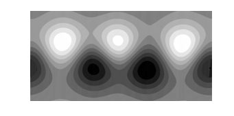
$t=5$

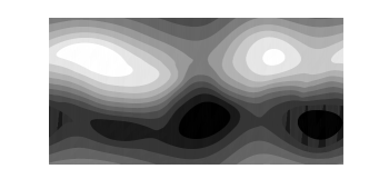
$t=10$

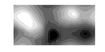
$t=15$

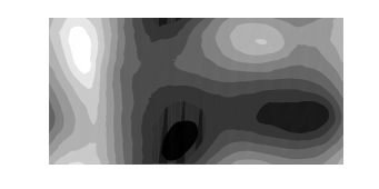
Figure 4: Contour plot of centre plane stream function $\psi$ for $\xi$=0.01. Light colours represent positive values of $\psi$, dark colours represent negative values.

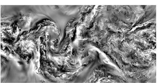
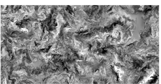
Figure 5: Centre plane ($z=0$) vertical velocity for $\xi=0.01$ (upper plot) and no stratification (lower plot) at $t=10$. Dark colours represent negative (downward) velocity, light colours represent positive velocity.

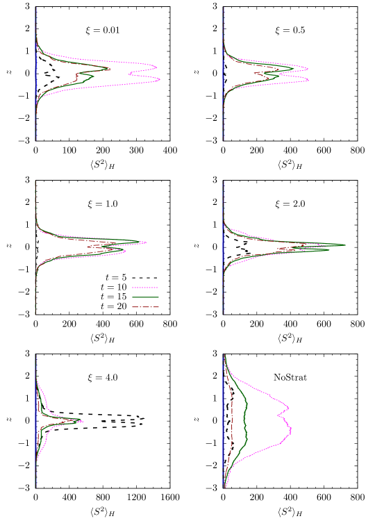
Figure 6: Time evolution of $\left<{S^{2}}\right>_{H}$ for several $\xi$ and no density stratification simulations. Note that the horizontal scale is not the same for all the plots.

In stratified flows dominated by vortical modes, such as those simulated in this study, it is postulated that horizontal layer decoupling occurs and that the flow will be susceptible to Kelvin-Helmholtz shear instabilities (Lilly, 1983). The square of the vertical shear of horizontal motions is defined as:

$$S^{2}=\left(\frac{\partial u}{\partial z}\right)^{2}+\left(\frac{\partial v}{\partial z}\right)^{2}\,.$$ (7)

Figure 6 contains plots of the horizontally averaged square of vertical shear $\left<{S^{2}}\right>_{H}$ versus vertical position for several $\xi$ and the non-stratified simulation, where $\left<{\cdot}\right>_{H}$ denotes averaging over $xy$-planes. Initially, the shear profile demonstrates a bimodal pattern, with maximum values at $z\pm 0.5$, and is a result of the initial sech${}^{2}(z)$ velocity profile. For all the stratified cases the bimodal maximum shear pattern persists in time, but the peaks do not remain aligned with the peaks in the initial shear profile. Instead, the distance between peaks decreases in time as the peaks move toward the planes of maximum energy. This shift in the location of the maximum shear from that of the maximum shear in the initial conditions toward that of the maximum energy in the initial conditions is consisted with the results of Riley & de Bruyn Kops (2003), and suggests that the peak shear is due to decoupling of the horizontal motions as suggested by Lilly (1983) and not just from the initial conditions. In contrast, the bimodal pattern disappears by $t=5$ for the non-stratified case in which horizontal decoupling does not occur.

4 Location of Flows in Parameter Space

It has long been recongised that interpretation of simulation and laboratory results depends on understanding the flow regime they are in. For example, a flow that is marginally turbulent may provide limited information about flows at high Reynolds number. In stratified turbulence, non-dimensionalisation of the governing equations shows there are three dimensionless parameters which we take to be a Reynolds, a Froude, and a Schmidt number in writing (5). Recently, de Bruyn Kops & Riley (2019) showed that, for a given Schmidt or Prandtl number, the Froude number and activity parameter, also called the buoyancy Reynolds number, form a parameter space that is effective for interpreting a large number of historical laboratory experiments and recent simulations. Understanding the location of the current simulations in this parameter space is the subject of this section in order to prepare for interpreting the flows in §5

The motivation for choosing Froude number and activity parameter as the axes on our parameter space for interpreting results is that turbulence is characterised by a range of length scales. In stratified turbulence, there can be scales of motion strongly effected by buoyancy, strongly affected by viscosity, and not affected significantly by either. Let us consider ratios of three length scales denoted $L$, $L_{o}$, and $L_{k}$. The most appropriate definitions of these may be open questions, but conceptually they describe, respectively, the scale of the turbulent kinetic energy, the largest scale that is not directly affected by buoyancy, and the dissipation scale. In this context, an inverse Froude number is indicative of the scale separation between $L$ and $L_{o}$ while the activity parameter is indicative of the scale separation between $L_{o}$ and $L_{k}$. Particularly in simulations, since the total scale separation is quite limited, it is informative to consider length scale ratios when evaluating simulation results.

For specificity, and for comparison with the literature, let us define

$$\tilde{L}=\frac{\tilde{k}^{3/2}}{\widetilde{\epsilon}}\>,\hskip 28.45274pt\tilde{L}_{o}=\left(\frac{\widetilde{\epsilon}}{\widetilde{\mathit{N}}^{3}(\tilde{z})}\right)^{1/2}\>,\hskip 28.45274pt\tilde{L}_{k}=\left(\frac{\tilde{\nu}^{3}}{\widetilde{\epsilon}}\right)^{1/4}$$ (8)

where $\widetilde{\mathit{N}}^{2}(\tilde{z})=\tilde{g}/\tilde{\rho}_{0}d\tilde{\overline{\rho}}(\tilde{z})/d\tilde{z}$ is the buoyancy frequency at vertical position $\tilde{z}$, so that

$${Fr}=\left(\frac{\tilde{L}}{\tilde{L}_{o}}\right)^{-2/3}=\frac{\widetilde{\epsilon}}{\widetilde{\mathit{N}}(\tilde{z})\tilde{k}}\>,\hskip 28.45274pt{Gn}=\left(\frac{\tilde{L}_{o}}{\tilde{L}_{k}}\right)^{4/3}=\frac{\widetilde{\epsilon}}{\tilde{\nu}\widetilde{\mathit{N}}^{2}(\tilde{z})}\ .$$ (9)

${Fr}$ is the turbulence Froude number while ${Gn}$ is the activity parameter, also called the buoyancy Reynolds number. In some literature, the latter term is used for the product of the square of the horizontal Froude number and the horizontal Reynolds number, introduced by Riley & de Bruyn Kops (2003), which is not the same as ${Gn}$ unless certain inertial scaling assumptions hold (c.f. de Bruyn Kops & Riley, 2019). To avoid confusion between the two quantities, we use the original name, activity parameter, for ${Gn}$ (e.g. Dillon & Caldwell, 1980); the symbol is in deference to the introduction of this quantity by Gibson (1980) and to its identification by Gargett et al. (1984) as a measure of the dynamic range available for turbulence at scales too small to be directly affected by buoyancy.

The observation that stratified flow dynamics depend strongly on ${Fr}$ and ${Gn}$ has been the subject of many studies. For example ${Fr}$ must be sufficiently small for the scaling arguments of Billant & Chomaz (2001) and Riley & de Bruyn Kops (2003) to hold. Brethouwer et al. (2007) describe a ‘strongly’ stratified regime corresponding to $Fr\sim O(0.01)$ or smaller, and Falder et al. (2016) refer to this regime as ‘layered anisotropic stratified turbulence’ (LAST) to avoid ambiguity of the meaning of ‘strongly stratified.’ Diamessis et al. (2011) report strong effects of buoyancy on stratified turbulent wakes for values of ${Fr}$ (inferred from their data) significantly above that of the LAST regime. Almalkie & de Bruyn Kops (2012) report the characteristics of homogeneous stratified turbulence in the LAST regime and less strongly stratified, and provide a conversion chart between various Froude numbers for their data. Note that the conversion between $L$ and the integral, or correlation, length scale is dependent on Froude number (de Bruyn Kops, 2015; Maffioli & Davidson, 2016) so that a generic conversion between Froude numbers is not practical.

The history of the importance of ${Gn}$ to parametrise the dynamics of stratified turbulence goes back farther. Using scaling arguments, Gibson (1980) estimated that ${Gn}\approx 24$ is the minimum value for “active” turbulence to form. This estimate was soon followed with ocean measurements showing that markedly differing flow regimes correspond to different ranges of ${Gn}$ (Gargett et al., 1984). Since then, multiple studies have been focused on the importance of correctly accounting for the effect of ${Gn}$, and not just for Froude and Reynolds number, in simulations (Smyth & Moum, 2000a; Almalkie & de Bruyn Kops, 2012; Bartello & Tobias, 2013). Based on simulations with domain-averaged ${Gn}=$ 13, 50, and 220, Portwood et al. (2016) propose modeling a stratified turbulent flow as an amalgamation of flow regimes distinguished by the ${Gn}$ averaged over subregions of the flow. They conclude that regions with locally averaged ${Gn}$ of $O(1)$, $O(10)$, and $O(100)$ are dynamically distinct, which is consistent with the ocean measurements of Gargett et al. (1984). Recently, de Bruyn Kops & Riley (2019) use new simulations and historical laboratory data to show that the time-evolution of decaying flows depends strongly on ${Gn}$. In particular, viscous effects are important when ${Gn}\sim 10$ and dominate when ${Gn}\sim 1$. Finally, we note that the stratified late wakes of Watanabe et al. (2016) with ${Gn}$ on centreline of $O(10)$ evolve differently from simulated and laboratory wakes with lower centreline ${Gn}$.

To understand ${Fr}$ and ${Gn}$ in the context of non-uniform stratification, we consider domain-averages and planar-averages:

$$\left<{Fr}\right> =\frac{\left<{\widetilde{\epsilon}}\right>}{\widetilde{\overline{\mathit{N}}}\left<{\tilde{k}}\right>}\ , \left<{Gn}\right> =\frac{\left<{\widetilde{\epsilon}}\right>}{\tilde{\nu}\widetilde{\overline{\mathit{N}}}^{2}}\ ,$$ (10)

$$\left<{Fr}\right>_{H} =\frac{\left<{\widetilde{\epsilon}}\right>_{H}}{\tilde{N}\left<{\tilde{k}}\right>_{H}}\ , \left<{Gn}\right>_{H} =\frac{\left<{\widetilde{\epsilon}}\right>_{H}}{\tilde{\nu}\widetilde{\mathit{N}}^{2}(\tilde{z})}\ .$$ (11)

The time evolutions of the domain averaged quantities are plotted in figure 7.

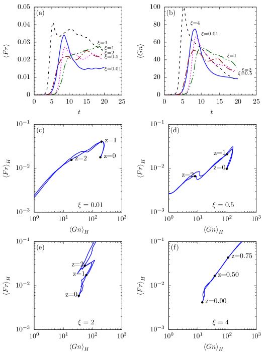
Figure 7: Panels (a) and (b): time evolution of domain-averaged ${Fr}$ and ${Gn}$. Panels (c), (d), (e), (f): location of each plane in $\left<Gn\right>_{H}-\left<Fr\right>_{H}$ space at $t=10$ for four of the five cases with three planes marked with dots for each case; one curve in each panel is for the top half of the wake ($z\geq 0$) and the other curve for the bottom half of the wake.

The plot of $\left<Fr\right>$ in figure 7(a) might suggest that the flows are strongly stratified but perhaps not in the LAST regime, and to the plot of $\left<Gn\right>$ that the flows consist of patches of turbulence by the criteria of Portwood et al. (2016). These conclusions are called into question, though, after reconsideration of how $N$ and $\epsilon$ vary in the vertical. For this reason, parameter maps for four of the cases at $t=10$ are included in figure 7 as panels (c), (d), (e), and (f). Time $t=10$ is chosen because there has been sufficient time for the flows to develop but they are still highly energetic (c.f. figure 5). From these panels, it is apparent that there are regions of the flow in the LAST regime ($Fr\lesssim O(0.01)$) and regions not in the LAST regime both over a significant range of $Gn$.

Figure 7 gives our first understand of fundamental difference between flows with nearly uniform stratification and those with sharply varying stratifications. In panels (c) and (d) of the figure, which are the flows with the most nearly uniform stratification, $Gn$ is highest on the centreline and decreases toward the edges. $Fr$ is also highest in the wake core and decreases toward the edges. This is because the stratification is significant at the edges so that it, combined with the lack of wake energy, results in very low turbulence. In panels (e) and (f), which are flows with strong variation in stratification, the opposite is true because for $\xi=2$ and $4$ the stratification is so weak at the edges that the turbulence is high. In all cases, though, the location in the $\left<Fr\right>_{H}-\left<Gn\right>_{H}$ plane indicate that all the wake cores are in the LAST regime by the criteria of Brethouwer et al. (2007) and dominated by three-dimensional turbulence by the criteria of de Bruyn Kops (2015) and Portwood et al. (2016).

5 Energetics and Mixing

In figure 7 we observe that the layout of the wake in parameter space when $\xi$ is low is different from that when $\xi$ is high. This suggests that the mixing characteristics will be different for different $\xi$. To explore this, we consider energy and mixing in this section.

5.1 Kinetic Energy

The horizontal and vertical contributions to kinetic energy are defined as:

$$e_{H}=\frac{1}{2}\left(u^{2}+v^{2}\right)\ ,\quad e_{V}=\frac{1}{2}\left(w^{2}\right)\ .$$

These are local quantities. An overview of the flow energetics is given by the the $x$-direction spectrum of horizontal energy defined as

$$E_{H}(k_{x})=\frac{1}{2}\left(\widehat{u}(k_{x})\widehat{u}(k_{x})^{*}+\widehat{v}(k_{x})\widehat{v}(k_{x})^{*}\right)\,.$$

Here $\widehat{u}(k_{x})$ and $\widehat{v}(k_{x})$ are the $x$ and $y$ components of velocity Fourier transformed in the $x$-direction, $(\cdot)^{*}$ denotes a complex conjugate, and $k_{x}$ is the $x$-direction wave number. Figure 8(a) contains a plot of the time evolution of $\widehat{E}_{H}(k_{x})$ for $\xi=1$, which is representative of the spectra of all simulations conducted in this study. The initial peak at $k_{x}\approx\pi/2$ corresponds to the separation distance between vortices. As the flow evolves, transfer of energy to smaller scales is observed as the magnitude of $\widehat{E}_{H}(k_{x})$ at larger wave numbers increases between $t=0$ and $t=10$. After $t=10$, the flow is fully developed in the sense that the energy at all wave numbers decreases for $t>10$. In addition, once the flow has had time to develop from the initial conditions ($t>10$), it displays a $k_{x}^{-5/3}$ spectrum spanning a decade of $k_{x}$. This $k_{x}^{-5/3}$ dependence is seen for all $\xi$ in figure 8(b). Other simulations have exhibited approximately $k_{x}^{-5/3}$ spectra (Riley & de Bruyn Kops, 2003; Lindborg, 2006; Bartello & Tobias, 2013), but it has been observed that slopes tend to be flatter than $k_{x}^{-5/3}$ for low Froude number (Bartello & Tobias, 2013; de Bruyn Kops, 2015) although the results of de Bruyn Kops (2015) and de Bruyn Kops & Riley (2019) indicate that low $Gn$ affects the spectral slope and that, in sets of simulations, it is often difficult to distinguish the effects of $Fr$ from those of $Gn$.

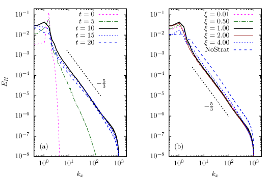
Figure 8: (a) Evolution of $E_{H}(k_{x})$ $\xi=1$; (b) $E_{H}(k_{x})$ $x$ spectrum for all $\xi$ at $t=10$. The curves in (b) for the stratified cases are almost indistinguishable except near the left edge where they go in this order from bottom to top: NoStrat, 4.00, 0.01, 0.50 1.00, 2.00.

The time evolution of $\left<{e_{H}}\right>$ and $\left<{e_{V}}\right>$ for each $\xi$ are shown in figure 9.

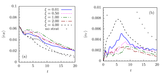
Figure 9: Time evolution of the average (a) horizontal and (b) vertical contributions to kinetic energy.

As $\xi$ is increased from 0.01 to 2, the trend is for $\left<{e_{H}}\right>$ to persist longer in time and the magnitude of $\left<{e_{V}}\right>$ to decrease compared with the unstratified flow. In contrast, the case with $\xi=4$ loses very nearly the same amount of energy between $t=0$ and $t=20$ as the unstratified cases, and it loses approximately 83% of its energy in this time compared with approximately 58% for the other cases. The case with $\xi=4$ also creates a lot of vertical motion as indicated by the plot of $\left<{e_{V}}\right>$ in figure 9(b).

To understand why the case with $\xi=4$ evolves markedly differently from the other cases, we present the vertical profiles of $\left<{e_{V}}\right>_{H}$ for $\xi=2$ and $\xi=4$ in figure 10. With $\xi=2$, most of the vertical motion is in the region where the mean density gradient is fairly strong whereas in $\xi=4$ the vertical motion is strongest outside the strongly stratified region. It appears that with $\xi=4$ that the regions above and below the strongly stratified zone act as unstratified wakes that decay faster than the stratified wakes.

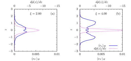
Figure 10: $\left<{e_{V}}\right>_{H}$ at $t=10$ for $\xi=2$ and $\xi=4$.

5.2 Available Potential Energy

Discussion of potential energy usually involves the concepts of available and background potential energy introduced by Lorenz (1955). He noted that in order to convert the total potential energy in the Earth’s atmosphere to kinetic energy, the temperature needed to reach absolute zero and all mass needed to be located at sea level. Instead, the potential energy that is available for conversion to kinetic energy, $E_{a}(t)$, is defined to be the result of any deviation from a background (or reference) potential energy, $E_{b}(t)$, defined as the potential energy that would occur if the fluid were adiabatically redistributed to a minimum energy state. The available potential energy is the total potential energy, $E_{p}(t)$, minus the background potential energy:

$$E_{a}(t)=E_{p}(t)-E_{b}(t)\,.$$ (12)

$E_{a}$ is a time varying quantity for a volume of fluid and each fluid element in the volume contributes to it and so one can define the local available potential energy, $e_{a}$, such that

$$E_{a}(t)=\int_{\mathcal{V}}e_{a}(\vec{x},t)d{\mathcal{V}}$$

is the available potential energy for some volume ${\mathcal{V}}$. Several papers discuss how $e_{a}$ must be defined so that it is fully consistent with the concept of available potential energy (Holliday & McIntyre, 1981; Roullet & Klein, 2009; Molemaker & McWilliams, 2010; Winters & Barkan, 2013).

A subtle concept is that $e_{a}$ is a local quantity that is affected by non-local changes in the density field via the effect of those non-local changes on the instantaneous reference state. Consider a fluid parcel with density $\rho_{t}(\vec{x},t)$. If all the fluid parcels in some volume are adiabatically sorted to find the reference configuration having minimum potential energy, $\rho_{\ast}(z,t)$, then that fluid parcel will move to a new location $z_{*}$. Alternatively, the parcel is elevated a distance $\zeta=z-z_{*}$ from the location it would occupy in the minimum energy arrangement. The local available potential energy is not proportional to $\rho\zeta$, though, because all the fluid parcels with sorted locations between $z$ and $z_{*}$ affect $e_{a}(\vec{x},t)$. Therefore,

$$e_{a}(\vec{x},t)=\left(\frac{2\pi}{\overline{\mathrm{Fr}}}\right)^{2}\left[\zeta\rho(\vec{x},t)-\int_{z_{*}}^{z}\rho(z^{\prime}_{*})dz^{\prime}\right]\ .$$ (13)

This expression is equivalent to that derived by Roullet & Klein (2009), and Winters & Barkan (2013) shows that it is positive semi-definite and integrates to $E_{a}$. We evaluate it numerically by sorting the density field with an algorithm that allows $\zeta$ to be recovered and by computing the integral in the expression via the trapezoid rule.

Before moving on to analysing potential energy in the simulations, let us define for convenience some notation regarding densities. The total density is

$$\rho_{t}(\vec{x},t)=\overline{\rho}(z)+\rho(\vec{x},t)$$ (14)

where an arbitrary additive constant has been omitted. The excess density relative to the reference density is

$$\rho_{e}(\vec{x},t)=\rho_{t}(\vec{x},t)-\rho_{\ast}(z,t).$$ (15)

If the flow is inviscid then $\rho_{e}=\rho$ and if the mean density profile is given by (3) then

$$e_{a}=\left(\frac{2\pi}{\overline{\mathrm{Fr}}}\right)^{2}\left[\rho_{t}\mathrm{arctanh}\left(\frac{\varrho\rho}{\varrho^{2}-\overline{\rho}\rho-\overline{\rho}^{2}}\right)+\frac{\varrho}{2}\ln\left(\frac{\varrho^{2}-(\rho_{t})^{2}}{\varrho^{2}-\overline{\rho}^{2}}\right)\right]\,,$$ (16)

where $\varrho=\Delta\rho/2$, independent of time (Hebert, 2007).

The time evolution of $\left<{e_{a}}\right>$ for each $\xi$ is shown in in figure 11(a).

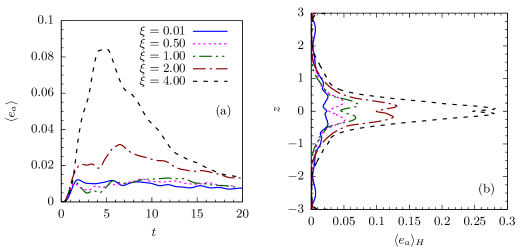
Figure 11: Evolution of (a) $\left<{e_{a}}\right>$; (b) $\left<{e_{a}}\right>_{H}$ at $t=10$ for each $\xi$.

These data are computed by sorting the fields to determine the background potential energy and then subtracting it from the total potential energy. The notation $\left<{e_{a}}\right>$ is used in order to be consistent with that for kinetic energy, but note that $\left<{e_{a}}\right>=E_{a}(t)$. Evident from the figure is that the case with $\xi=4$ generates significantly more available potential energy than the other cases, which is the result of the higher vertical motion in this case evident from figure 9.

The vertical profiles of $\left<{e_{a}}\right>_{H}$ are shown in figure 11(b). The bulk of the available potential energy in all cases is in the wake core. This is interesting because we see in figure 9(b) that the majority of the vertical motion in the case with $\xi=4$ is outside the strongly stratified core. From figure 11(b), though, we observe that since the stratification is weak in the region of the strongest vertical motion there is little potential energy associate with it. We conclude that, even though most of the potential energy is in the strongly stratified regions, the higher vertical motion with $\xi=4$ results in higher potential energy.

Also from figure 11(b) we observe a weakness in our analysis technique based on computing the local available potential energy $e_{a}$. In the paragraph preceding (13) it is observed that, while $e_{a}$ is a local quantity, it is affected by all the other fluid parcels in the sorting volume used for determining the background potential energy. In this case, we have defined the sorting volume as the entire computational domain, which is entirely arbitrary because we could simulate the wakes in a different size domain. An artifact of this arbitrariness is that extreme tails in the profiles of $\left<{e_{a}}\right>_{H}$ exhibit values that are higher than at some locations closer to the center of the wake. This happens because the numerical domain limits the elevations to which the fluid elements can sort. Even without the effects of a sorting volume with arbitrary height, we should consider the horizontal extent of the sorting. By our method, a fluid parcel on the left side of the domain can sort to a location on the right side of the domain. Taylor et al. (2019) compute available potential energy by sorting columns with horizontal extent of just a few Kolmogorov length scales. While we point out that there are other ways to interpret Lorentz’s concept of available potential energy in these simulations, the quantities in figure 11 are computed consistently for all the cases and we find them useful for understanding the effects of $\xi$ on energetics, at least conceptually.

5.3 Dissipation Rates and Mixing Efficiency

Mixing is a microscopic process affecting the thermodynamic state of a fluid. It is irreversible since the fluid cannot be returned to its original, pre-mixed state without an interaction with the surroundings. Mixing is typically quantified by the dissipation rates of kinetic and potential energy. Here the kinetic energy dissipation rate $\epsilon$ is defined in the usual way for incompressible flows.

The potential energy dissipation rate, $\epsilon_{p}$, is the rate at which available potential energy is irreversibly dissipated to background potential energy. In some configurations, it might be approximated as proportional to the diffusive destruction of the variance of $\rho$, which is sometimes denoted $\chi$. $\epsilon_{p}$ and $\chi$ are equal only if the reference density profile (the profile with least potential energy) is equal to the ambient profile $\overline{\rho}(z)$. We can write an expression $\epsilon_{p}$ in terms of $\chi$ plus the difference between $\epsilon_{p}$ and $\chi$ but find it more informative to follow Scotti & White (2014) and write

$$\epsilon_{p}=-\frac{g}{\rho_{0}{Re_{r}}\mathrm{Sc}}(|\nabla\rho_{t}|^{2}\frac{dz}{d\rho_{\ast}}-|\nabla\rho_{\ast}|^{2}\frac{dz}{d\rho_{t}})\;.$$ (17)

The first term describes the positive-definite dissipation due to local irreversible dipycnal mixing (c.f. Salehipour et al., 2016). The second term shows that a fluid parcel can gain or lose available potential energy due to irreversible global changes in the reference density profile, that is, due to dipycnal mixing elsewhere in the volume of fluid for which the reference profile is defined.

Of general interest is how efficiently a flow mixes a scalar field. One measure of this is the mixing efficiency

$$\eta=\frac{\epsilon_{p}}{\epsilon_{p}+\epsilon}\,.$$ (18)

$\eta$ is of particular interest in field experiments because it is difficult to measure both $\epsilon$ and $\epsilon_{p}$ simultaneously. Thus, it is useful to measure one quantity (usually $\epsilon$) and relate it to the other (Osborn, 1980). Gregg et al. (2018) review $\eta$ in the context of ocean measurements and Taylor et al. (2019) use DNS data to analyze some of the underlying assumptions in estimating and applying $\eta$. Here we compute the volume-averaged mixing efficiency $\left<{\eta}\right>=\left<{\epsilon_{p}}\right>/\left<{\epsilon_{p}+\epsilon}\right>$ directly from the simulation data.

The evolutions in time of the boxed-averaged dissipation rates and mixing efficiency are plotted as figure 12.

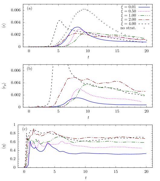
Figure 12: Time evolution of dissipation rates and mixing efficiency.

Recall that the flows are initialised with no small-scale motions and so at $t=0$ $\left<{\epsilon}\right>$ is very small and $\left<{\epsilon_{p}}\right>$ is zero. As the flows evolve, small scale turbulence forms and the dissipation rates increase in time before decaying. Any stratification, regardless of $\xi$, reduces $\left<{\epsilon}\right>$ relative to the unstratified case, which is consistent with Almalkie & de Bruyn Kops (2012) and de Bruyn Kops & Riley (2019) for flows that are not viscously dominated. There is a weak trend for higher $\xi$ to retard the development of $\left<{\epsilon}\right>$, except when $\xi=4$, in which case $\left<{\epsilon}\right>$ increases even faster than it does for the unstratified case. In all the stratified cases, $\left<{\epsilon_{p}}\right>$ follows $\left<{\epsilon}\right>$ fairly closely so that $\left<{\eta}\right>$ quickly rises to close to its steady state value, and in all cases has settled to the steady value by about $t=10$.

Considering mixing efficiency further, from figure 12(e,f) it is seen that $\left<{\eta}\right>$ settles by about $t=10$ to much different values when $\xi<2$ and $\xi\geq 2$. For low $\xi$, $\left<{\eta}\right>\approx 0.35$, which is consistent with simulated flows with $\mathrm{Sc}=1$ (Riley & de Bruyn Kops, 2003; Almalkie & de Bruyn Kops, 2012; de Bruyn Kops & Riley, 2019). The laboratory experiments of Liu (1995) indicate a value of 0.41 whereas Maffioli & Davidson (2016) find 0.25 for very low Froude number and Osborn (1980) assumed 0.17 based on ocean data. The latter value may be explained by the effects of Schmidt (or Prandtl) number (c.f. Smyth et al., 2001; Salehipour & Peltier, 2015) or by the effects of forcing from strong vertical mean shear (Portwood et al., 2019).

For the simulations with $\xi\geq 2$, $\left<{\eta}\right>\approx 0.65$ when $t>10$. Two other flows with similarly high $\eta$ is horizontal convection with $\left<{\eta}\right>=0.85$ (Scotti & White, 2011) and Rayleigh-Taylor and $\left<{\eta}\right>=0.5$ (Dalziel et al., 2008). It is not obvious that either of these configurations relates to ours except, perhaps, that they all generate significant vertical motion. Consider again figures 9 and 10 in which we observe that vertical motion is induced outside the strongly stratified region, particularly when $\xi=4$, and results in high $E_{a}$ when that motion does work against the strong density gradient near the centreline. This phenomenon is less pronounced when $\xi=2$, but, nevertheless, apparent.

6 Modelling Implications and Conclusions

Simulation results are presented for flows initialised with a von Kármán vortex street and no mean velocity or shear, similar to a momentumless wake. Each simulation is subject to non-uniform density stratification to represent a wake in natural settings such as that found in an atmospheric transition layer or thermohaline staircase. The average stratification for all the cases is the same so the only simulation parameter that is adjusted is $\xi$, the ratio of the wake height to the stratification profile height. The average stratification is strong enough so that the average Froude number is order one. Comparisons to the unstratified case are also made since it is observed that flows in which the density changes over a very short vertical range have certain characteristics more like those of unstratified than stratified flows.

The simulated flows in which the wake height is less than or equal to twice the density layer height ($\xi\leq 2$) are observed to be consistent with the current understanding of strongly stratified flow, in particular, increasing horizontal and decreasing vertical length scales as the flows evolve. These characteristics are in agreement with the scaling arguments of Riley et al. (1981) and the horizontal layer decoupling heuristic by Lilly (1983). When the wake height is greater that twice the density layer height ($\xi>2$), however, the importance of the density stratification is diminished and the flows demonstrate characteristics of non-stratified flows. In particular, horizontal contribution to kinetic energy $\left<{e_{H}}\right>$ dissipates faster, and the vertical contribution $\left<{e_{V}}\right>$, as well as the dissipation rates $\left<{\epsilon}\right>$ and $\left<{\epsilon_{p}}\right>$ increase much faster and to much higher values than in the cases with $\xi\leq 2$.

The transition point of $\xi\approx 2$ suggests that it is the relation between the stratification profile and the energy profile, rather than the velocity profile, that determines if the flow will behave primarily as stratified or unstratified in terms of global statistics. Rather than simply concluding that the observed results might be explained by energetics, it worthwhile to briefly consider instability mechanisms. The Kelvin-Helmholtz (KH) instability is typically assumed to be the dominant instability mechanism in stratified flows. In shear flows where the density length scale becomes smaller than the velocity length scale, however, theoretical analysis first performed by Holmboe (1962) showed an oscillatory instability. Evidence of the Holmboe instability has been observed in the atmosphere (e.g., Emmanuel et al., 1972) and ocean (e.g., Yonemitsu et al., 1996). Transition from KH to Holmboe instability has been investigated theoretically (e.g., Smyth & Peltier, 1989; Ortiz et al., 2002), experimentally (e.g., Zhu & Lawrence, 2001; Hogg & Ivey, 2003) and numerically (e.g., Hazel, 1972; Smyth et al., 1988). In particular, Smyth & Winters (2003) demonstrate that when the ratio of velocity to density length scales is greater than 2.4 then Holmboe instability becomes dominant. A significant difference between those experiments and ours is that our simulations have no mean shear. Also, we are considering the wake of an object rather than a shear plane. Nevertheless, the results of Smyth & Winters (2003) support our conclusion that stratified flow configurations with the equivalent of $\xi>2$ should not be expected to behave like uniformly stratified flows.

One motivation for studying flows subject to non-linear stratification is to improve ocean and atmospheric modelling. The results of this study suggest that modelling a sharp localised density gradient with a uniform density profile having the same average density gradient will result in underpredicting $\left<{\epsilon_{p}}\right>$ by a factor of two or more with a corresponding underprediction of the mixing efficiency.