A posteriori verification of the positivity of solutions to elliptic boundary value problems

Abstract

The purpose of this paper is to develop a unified a posteriori method for verifying the positivity of solutions of elliptic boundary value problems by assuming neither $H^{2}$-regularity nor $L^{\infty}$-error estimation, but only $H^{1}_{0}$-error estimation. In [J. Comput. Appl. Math, Vol. 370, (2020) 112647], we proposed two approaches to verify the positivity of solutions of several semilinear elliptic boundary value problems. However, some cases require $L^{\infty}$-error estimation and, therefore, narrow applicability. In this paper, we extend one of the approaches and combine it with a priori error bounds for Laplacian eigenvalues to obtain a unified method that has wide application. We describe how to evaluate some constants required to verify the positivity of desired solutions. We apply our method to several problems, including those to which the previous method is not applicable.

1 Introduction

In recent decades, numerical verification (also known as computer-assisted proof, validated numerics, or verified numerical computation) has been developed and applied to various partial differential equations, including those where purely analytical methods have failed (see, for example, plum1992explicit ; day2007validated ; plum2008 ; mckenna2009uniqueness ; nakao2011numerical ; mckenna2012computer ; takayasu2013verified ; nakaoplumwatanabe2019numerical ; tanaka2020numerical and the references therein). One such successful application is to the semilinear elliptic boundary value problem

$$\left\{\begin{array}[]{ll}-\Delta u=f(u)&\text{in}~{}\Omega,\\ u=0&\text{on}~{}\partial\Omega,\end{array}\right.$$ (3)

where $\Omega\subset\mathbb{R}^{N}$ $(N=2,3,\cdots)$ is a given bounded domain, $\Delta$ is the Laplacian, and $f:\mathbb{R}\rightarrow\mathbb{R}$ is a given nonlinear map. Further regularity assumptions for $\Omega$ and $f$ will be shown later for our setting.

Positive solutions of (3) have attracted significant attention lions1982existence ; gidas1979symmetry ; lin1994uniqueness ; damascelli1999qualitative ; gladiali2011bifurcation ; de2019morse . For example, positive solutions of problem (3) with $f(t)=\lambda t+t|t|^{p-1}$, $\lambda\in[0,\lambda_{1}(\Omega))$, $p\in(1,p^{*})$ have been investigated from various points of view such as uniqueness, multiplicity, nondegeneracy, and symmetry, gidas1979symmetry ; lin1994uniqueness ; damascelli1999qualitative ; gladiali2011bifurcation ; de2019morse , where $p^{*}=\infty$ when $N=2$ and $p^{*}=(N+2)/(N-2)$ when $N\geq 3$; $\lambda_{1}(\Omega)$ is the first eigenvalue of $-\Delta$ with the homogeneous Dirichlet boundary value condition in the weak sense. Another important nonlinearity is $f(t)=\lambda(t-t^{3})$, $\lambda>0$. This corresponds to the stationary problem of the Allen–Cahn equation allen1979microscopic . The problem (3) with this nonlinearity may have a positive solution when $\lambda\geq\lambda_{1}(\Omega)$. However, when $\lambda<\lambda_{1}(\Omega)$, no positive solution is admitted; this can be confirmed by multiplying $-\Delta u=\lambda(u-u^{3})$ with the first eigenfunction of $-\Delta$ and integrating both sides. The Allen–Cahn equation is a special case of the Nagumo equation mckean1970nagumo with the nonlinearity $f(t)=\lambda t(1-t)(t-a)$, $\lambda>0$ and $0<a<1$, and both of these equations have been investigated by many researchers. We are moreover interested in the related case in which $f(t)=\lambda(t+At^{2}-Bt^{3})$ with $A,B>0$. The bifurcation of problem (3) with this nonlinearity was analyzed in lions1982existence . This problem has two positive solutions when $\lambda^{*}<\lambda<\lambda_{1}(\Omega)$ for some $\lambda^{*}>0$. Despite these results, quantitative information about the positive solutions, such as their shape, has not been clarified analytically. Throughout this paper, $H^{k}(\Omega)$ denotes the $k$th order $L^{2}$ Sobolev space. We define $H^{1}_{0}(\Omega):=\{u\in H^{1}(\Omega):u=0~{}\mbox{on}~{}\partial\Omega\}$, with the inner product $(u,v)_{H^{1}_{0}}:=(\nabla u,\nabla v)_{L^{2}}$ and norm $\|u\|_{H^{1}_{0}}:=\sqrt{(u,u)_{\smash{H^{1}_{0}}}}$.

Numerical verification methods enable us to obtain an explicit ball containing exact solutions of (3). More precisely, for a numerical approximation $\hat{u}\in H^{1}_{0}(\Omega)$ that satisfies the assumption required by such methods, they prove the existence of an exact solution $u\in H^{1}_{0}(\Omega)$ of (3) that satisfies

$$\left\|u-\hat{u}\right\|_{H_{0}^{1}}\leq\rho$$ (4)

with an explicit error bound $\rho>0$. Under an appropriate condition, we can obtain an $L^{\infty}$-estimation

$$\left\|u-\hat{u}\right\|_{L^{\infty}}\leq\sigma$$ (5)

with bound $\sigma>0$. For instance, when $u,\hat{u}\in H^{2}(\Omega)$, we can evaluate the $L^{\infty}$-bound $\sigma>0$ by considering the embedding $H^{2}(\Omega)\hookrightarrow L^{\infty}(\Omega)$ (plum1992explicit, , Theorem 1 and Corollary 1). Thus, these approaches have the advantage that quantitative information about a target solution is provided accurately in a strict mathematical sense. We can identify the approximate shape of solutions from the error estimates. Despite these advantages, information about the positivity of solutions is not guaranteed without further considerations, irrespective of how small the error bound ($\rho$ or $\sigma$) is. In the homogeneous Dirichlet case (3), it is possible for a solution that is verified by such methods to be negative near the boundary $\partial\Omega$.

Therefore, we developed methods of verifying the positivity of solutions of (3) in previous studies tanaka2015numerical ; tanaka2017numerical ; tanaka2017sharp ; tanaka2020numerical and applied these result to sing-changing solutions tanaka2021posteriori . These methods succeeded in verifying the existence of positive solutions by checking simple conditions. In tanaka2015numerical ; tanaka2017numerical ; tanaka2017sharp , we proposed methods for verifying the positivity of solutions of (3) by assuming both error estimates (4) and (5). Subsequently, in tanaka2020numerical , we extended our method to a union of two different approaches (tanaka2020numerical, , Theorems 2.1 and 3.2) under certain conditions for nonlinearity $f$. Table 1 summarizes the error-estimate types that are required by these theorems when $f$ is a subcritical polynomial

$$f(t)=\lambda t+\sum_{i=2}^{n(<p^{*})}a_{i}t|t|^{i-1},~{}~{}\lambda,~{}a_{i}\in\mathbb{R},~{}a_{i}\neq 0\text{~{}~{}for~{}some~{}~{}}i.$$ (6)

Theorem 2.1 in tanaka2020numerical can be applied to cases in which $\lambda<\lambda_{1}(\Omega)$. This theorem is based on the constructive norm estimation for the minus part $u_{-}:=\max\{-u,0\}$ of a solution $u$, and does not assume an $L^{\infty}$-estimation (5) but only requires an $H^{1}_{0}$-error estimation (4). When $a_{i}\leq 0$ for all $i$ and $\lambda\geq\lambda_{1}(\Omega)$, we used a completely different approach (tanaka2020numerical, , Theorem 3.2) that was based on the Newton iteration that retains nonnegativity. This theorem needs no $L^{\infty}$-estimation but requires an explicit evaluation of the minimal eigenvalue of a certain linearized operator around approximation $\hat{u}$. Actually, this eigenvalue evaluation itself is not trivial to obtain. In tanaka2020numerical , the eigenvalue was estimated using the existing method tanaka2020numerical ; liu2015framework based on Galerkin approximations. Theorems 2.1 and 3.2 in tanaka2020numerical were applied numerically to problem (3) with the above-mentioned nonlinearities: $f(t)=\lambda t+t|t|^{p-1}$ and $f(t)=\lambda(t-t^{3})$. However, a problem still remains in the sense that we need the $L^{\infty}$-error estimation (5) to prove positivity when $a_{i}a_{j}<0$ for some $i,j$ and $\lambda\geq\lambda_{1}(\Omega)$. For example, the nonlinearity $f(t)=\lambda(t+At^{2}-Bt^{3})$ in which we are interested requires such an estimation. These requirements may narrow the applicability of the methods because the existing approach provided in (plum1992explicit, , Theorem 1 and Corollary 1) requires $u,\hat{u}\in H^{2}(\Omega)$, evaluating the bound for the embedding $H^{2}(\Omega)\hookrightarrow L^{\infty}(\Omega)$, to obtain $\sigma$ from $\rho$. The $H^{2}$-regularity of $u$ may fall when $\Omega$ is a nonconvex polygonal domain.

Table 1: Error estimates required in tanaka2020numerical when $f$ is the subcritical polynomial (6).

$a_{i}$	$\lambda$
	$\geq\lambda_{1}(\Omega)$	$<\lambda_{1}(\Omega)$
$a_{i}\geq 0$ for all $i$	No positive solution	(4), (tanaka2020numerical, , Theo. 2.1)
$a_{i}\leq 0$ for all $i$	(4), (tanaka2020numerical, , Theo. 3.2)	No positive solution
$a_{i}a_{j}<0$ for some $i,j$	(4) and (5), (tanaka2020numerical, , Cor. A.1)	(4), (tanaka2020numerical, , Theo. 2.1)

The purpose of this paper is to develop a unified method for verifying the positivity of solutions $u$ of (3) by assuming neither $H^{2}$-regularity nor (5), but only $H^{1}_{0}$-error estimation (4), which can be applied to all the cases in Table 1 for arbitrary bounded domains $\Omega$. Our method is based on a posteriori constructive norm estimation for the minus part $u_{-}$ and can be regarded as an extension of (tanaka2020numerical, , Theorem 2.1). In short, we confirm that the norm of $u_{-}$ vanishes by checking certain inequalities while assuming (4) (see Lemma 6.1). One of the key points is to estimate lower bounds of eigenvalue $\lambda_{1}(\text{\rm supp\,}u_{-})$ explicitly because the inequality $\lambda_{1}(\text{\rm supp\,}u_{-})\geq\lambda$ has to be confirmed for the success of our positivity proof (again, see Lemma 6.1). Here, $\text{\rm supp\,}u_{-}:=\overline{\{x\in\Omega:u_{-}(x)\neq 0\}}$ is the support of $u_{-}$, and $\lambda_{1}(\text{\rm supp\,}u_{-})$ is understood as the first eigenvalue on the interior of $\text{\rm supp\,}u_{-}$. When the interior of $\text{\rm supp\,}u_{-}$ is empty, we interpret $\lambda_{1}(\text{\rm supp\,}u_{-})=\infty$, and all real numbers are lower bounds of $\lambda_{1}(\text{\rm supp\,}u_{-})$. The difficulty is that we cannot identify the location and shape of $\text{\rm supp\,}u_{-}$ from (4) even when $\hat{u}$ is nonnegative.

If a polygon or polyhedron $S$ enclosing $\text{\rm supp\,}u_{-}$ is obtained concretely, we can apply the Liu–Oishi method liu2013verified ; liu2015framework based on finite element methods to obtain a lower bound for $\lambda_{1}(S)$. Then, the inequality $\lambda_{1}(\text{\rm supp\,}u_{-})\geq\lambda_{1}(S)$ gives the desired lower bound of $\lambda_{1}(\text{\rm supp\,}u_{-})$. Such a supremum set $S$ over $\text{\rm supp\,}u_{-}$ can be obtained when we have an $L^{\infty}$-estimation (5). By setting $\Omega_{+}:=\{x\in\Omega:\hat{u}-\sigma\geq 0\}$ where $u\geq 0$ therein, we can construct such a domain $S$ as a supremum set of $\Omega\backslash\Omega_{+}$. Again, we cannot determine such a supremum set $S$ only from $H^{1}_{0}$-error estimation (4). The Temple–Lehmann–Goerisch method can help us to evaluate $\lambda_{1}(\text{\rm supp\,}u_{-})$ more accurately (see, for example, (nakaoplumwatanabe2019numerical, , Theorem 10.31)).

To estimate the lower bound of $\lambda_{1}(\text{\rm supp\,}u_{-})$, we rely on the following argument:

Fact 1.1

For a bounded domain $\Omega\subset\mathbb{R}^{N}$ $(N=2,3,\cdots)$, there exists a constant $A_{k,N}$ independent of $\Omega$ such that

$$\lambda_{k}(\Omega)\geq A_{k,N}\left(\frac{1}{|\Omega|}\right)^{\frac{2}{N}},$$ (7)

where $\lambda_{k}(\Omega)$ denotes the $k$-th eigenvalue of $-\Delta$ with the homogeneous Dirichlet boundary condition.

Many articles have investigated this type of inequality in several forms. Among them, we mainly use the Rayleigh–Faber–Krahn inequality, which ensures Fact 1.1 for $k=1$ faber1923bweis ; krahn1925uber ; krahn1926uber . This inequality states that if $|\Omega|=|\Omega^{*}|$ ($\Omega^{*}$ is a ball in $\mathbb{R}^{N}$), then $\lambda_{1}(\Omega)\geq\lambda_{1}(\Omega^{*})$, where the equality holds if and only if $\Omega=\Omega^{*}$. We also refer to li1983schrodinger for an easy-to-estimate formula for $A_{k,N}$ for all $k\geq 1$ (see Remark 4.3). Section 4 provides explicit lower bounds of $A_{k,N}$ based on these results. To estimate a lower bound of $\lambda_{1}(\text{\rm supp\,}u_{-})$ using the inequality (7), we focus on estimating upper bounds of $|\text{\rm supp\,}u_{-}|$ while assuming only the $H^{1}_{0}$-error estimation (4) without knowing the specific shape and location of $\text{\rm supp\,}u_{-}$. Suppose that (4) is proved for a positive approximation $\hat{u}$ with sufficient accuracy. Then, the upper bound for $|\text{\rm supp\,}u_{-}|$ can be estimated very small using Lemma 3.2 provided later, and therefore, $\lambda_{1}(\text{\rm supp\,}u_{-})\geq\lambda$ can be confirmed using (7) for a moderately large $\lambda$. The established estimation for $|\text{\rm supp\,}u_{-}|$ is used to evaluate not only $\lambda_{1}(\text{\rm supp\,}u_{-})$ but also some Sobolev embedding constants on $|\text{\rm supp\,}u_{-}|$, which play an essential role for our positivity proof (again, see Lemma 6.1)

The remainder of this paper is organized as follows. Section 2 introduces required notation and definitions. In Section 3, we evaluate an upper bound for the volume $|\text{\rm supp\,}u_{-}|$ assuming the $H^{1}_{0}$-estimation (4) for a continuous or piecewise continuous approximation $\hat{u}\in H^{1}_{0}(\Omega)$. Subsequently, we use the bound for $|\text{\rm supp\,}u_{-}|$ to evaluate lower bounds for $\lambda_{1}(\text{\rm supp\,}u_{-})$ in Section 4. In Section 5, required Sobolev embedding constants on bounded domains are evaluated. In Section 6, we extend the previous formula (tanaka2020numerical, , Theorem 2.1) and combine it with the estimates derived from Sections 4 and 5, thereby designing a unified method for proving positivity. Finally, Section 8 presents numerical examples where the proposed method is applied to problem (3) with several nonlinearities, including those to which the previous method is not applicable without an $L^{\infty}$-error estimation.

2 Preliminaries

We begin by introducing required notation. We denote by $H^{-1}$ the topological dual of $H^{1}_{0}(\Omega)$. When describing norms and inner products, we may omit the domain of a function space unless there is a risk of misunderstanding. For example, we simply write $\|\cdot\|_{L^{p}}=\|\cdot\|_{L^{p}(\Omega)}$ if no confusion arises. For two Banach spaces $X$ and $Y$, the set of bounded linear operators from $X$ to $Y$ is denoted by ${\mathcal{L}}(X,Y)$ with the usual supremum norm $\|T\|_{{\mathcal{L}}(X,Y)}:=\sup\{\|Tu\|_{Y}/\|u\|_{X}:{u\in X\setminus\{0\}}\}$ for $T\in{\mathcal{L}}(X,Y)$. The norm bound for the embedding $H^{1}_{0}(\Omega)\hookrightarrow L^{p+1}\left(\Omega\right)$ is denoted by $C_{p+1}(=C_{p+1}(\Omega))$; that is, $C_{p+1}$ is a positive number that satisfies

$$\left\|u\right\|_{L^{p+1}(\Omega)}\leq C_{p+1}\left\|u\right\|_{H^{1}_{0}(\Omega)}~{}~{}~{}{\rm for~{}all}~{}u\in H^{1}_{0}(\Omega),$$ (8)

where $p\in[1,\infty)$ when $N=2$ and $p\in[1,p^{*}]$ when $N\geq 3$. If no confusion arises, we use the notation $C_{p+1}$ to represent the embedding constant on the entire domain $\Omega$, whereas, in some parts of this paper, we need to consider an embedding constant on some subdomain $\Omega^{\prime}\subset\Omega$. This is denoted by $C_{p+1}(\Omega^{\prime})$ to avoid confusion. Moreover, $\lambda_{1}(\Omega)$ denotes the first eigenvalue of $-\Delta$ imposed on the homogeneous Dirichlet boundary condition. This is characterized by

$$\lambda_{1}(\Omega)=\inf_{v\in H^{1}_{0}(\Omega)^{\backslash}{\{0\}}}\frac{\|v\|_{H^{1}_{0}(\Omega)}^{2}}{\|v\|_{L^{2}(\Omega)}^{2}}.$$ (9)

Throughout this paper, we assume that $f$ is a $C^{1}$ function that satisfies

$$|f(t)|\leq a_{0}|t|^{p}+b_{0}\text{~{}~{}~{}for~{}all~{}~{}}t\in\mathbb{R},$$ (10)

$$|f^{\prime}(t)|\leq a_{1}|t|^{p-1}+b_{1}\text{~{}~{}~{}for~{}all~{}~{}}t\in\mathbb{R}$$ (11)

for some $a_{0},a_{1},b_{0},b_{1}\geq 0$ and $p\in[1,p^{*})$. We define the operator $F$ as

$$F:\left\{\begin{array}[]{ccc}{u(\cdot)}&{\mapsto}&{f(u(\cdot))},\\ {H^{1}_{0}(\Omega)}&{\rightarrow}&{H^{-1}}.\end{array}\right.$$

Moreover, we define another operator $\mathcal{F}:H^{1}_{0}(\Omega)\rightarrow H^{-1}$ as $\mathcal{F}(u):=-\Delta u-F(u)$, which is characterized by

$$\left<\mathcal{F}(u),v\right>=\left(\nabla u,\nabla v\right)_{L^{2}}-\left<F(u),v\right>\text{~{}~{}for~{}all~{}~{}}u,v\in H^{1}_{0}(\Omega),$$ (12)

where $\left<F(u),v\right>=\int_{\Omega}f(u(x))v(x)dx$. The Fréchet derivatives of $F$ and $\mathcal{F}$ at $\varphi\in H^{1}_{0}(\Omega)$, denoted by ${F^{\prime}_{\varphi}}$ and ${\mathcal{F}^{\prime}_{\varphi}}$, respectively, are given by

$$\langle F^{\prime}_{\varphi}u,v\rangle=\int_{\Omega}f^{\prime}(\varphi(x))u(x)v(x)dx\text{~{}~{}for~{}all~{}~{}}u,v\in H^{1}_{0}(\Omega),$$ (13)

$$\langle\mathcal{F}^{\prime}_{\varphi}u,v\rangle=\left(\nabla u,\nabla v\right)_{L^{2}}-\langle F^{\prime}_{\varphi}u,v\rangle\text{~{}~{}for~{}all~{}~{}}u,v\in H^{1}_{0}(\Omega).$$ (14)

Under the notation and assumptions, we look for solutions $u\in H^{1}_{0}(\Omega)$ of

$$\mathcal{F}(u)=0,$$ (15)

which corresponds to the weak form of (3). We assume that some verification method succeeds in proving the existence of a solution $u\in H^{1}_{0}(\Omega)$ of (15) satisfying inequality (4) given $\hat{u}\in H^{1}_{0}(\Omega)$ and $\rho>0$. Although the regularity assumption for $\hat{u}$ (to be in $H^{1}_{0}(\Omega)$) is sufficient to obtain the error bound (4) in theory, we further assume that $\hat{u}$ is continuous or piecewise continuous throughout this paper. This assumption impairs little of the flexibility of actual numerical computation methods. We recall $u_{-}=\max\{-u,0\}$, and define $u_{+}:=\max\{u,0\}$.

3 Evaluation of the volume of $\text{\rm supp\,}u_{-}$

To estimate an upper bound for $|\text{\rm supp\,}u_{-}|$ from the information of the inclusion (4), we define $D(v):=\{x\in\Omega:\hat{u}(x)\leq v(x)\}$ and consider the maximization problem

$$\mathop{\rm maximize}\limits_{\left\|v\right\|_{L^{q}(\Omega)}=c}|D(v)|$$ (16)

for fixed $q\in(1,\infty)$ and $c>0$. This maximization takes place over the set of all functions $v\in L^{q}(\Omega)$ satisfying $\left\|v\right\|_{L^{q}(\Omega)}=c$. When $\left\|\hat{u}_{+}\right\|_{L^{q}(\Omega)}\leq c$, the maximal value of the problem (16) is $|\Omega|$. Therefore, we consider the case where $\left\|\hat{u}_{+}\right\|_{L^{q}(\Omega)}>c$. In the following, we denote $D(l):=\{x\in\Omega:\hat{u}(x)\leq l\}$ and $\mathring{D}(l):=\{x\in\Omega:\hat{u}(x)<l\}$ for $l\in\mathbb{R}$.

Lemma 3.1

Let $q\in(1,\infty)$ and $c>0$ be fixed. Suppose that $\left\|\hat{u}_{+}\right\|_{L^{q}(\Omega)}>c$. Then, we have

$$\mathop{\rm arg~{}max}\limits_{\left\|v\right\|_{L^{q}(\Omega)}=c}|D(v)|=\left\{\begin{array}[]{ll}\hat{u}_{+}(x),&x\in D,\\ 0,&\text{\rm otherwise},\end{array}\right.$$ (19)

where $D$ is a set that satisfies $\left\|\hat{u}_{+}\right\|_{L^{q}(D)}=c$ and

$$\mathring{D}(l)\subseteq D\subseteq D(l)$$ (20)

for some $l\in\mathbb{R}$. The maximal value of the problem (16) is $|D|$.

Proof

Let us denote by $v_{c}$ an arbitrary function in $\{v\in L^{q}(\Omega):\left\|v\right\|_{L^{q}(\Omega)}=c\}$. Because $D(v_{c})\subseteq D(|v_{c}|)$ and the equality holds when $v_{c}\geq 0$ in $\Omega$, the volume of $D(v_{c})$ is maximized for a nonnegative $v_{c}$.

Let $v_{c}$ be nonnegative. If $\hat{u}-v_{c}$ is strictly negative in some part $\Omega^{\prime}\subset\text{\rm supp\,}v_{c}$ satisfying $|\Omega^{\prime}|\neq 0$ and vanishes in $(\text{\rm supp\,}v_{c})\backslash\Omega^{\prime}$, another $v^{\prime}_{c}\in\{v\in L^{q}(\Omega):\left\|v\right\|_{L^{q}(\Omega)}=c\}$ with the same $c>0$ can be constructed to obtain larger $D(v^{\prime}_{c})$ as follows. Since $\left\|\hat{u}_{+}\right\|_{L^{q}(\Omega)}>c=\left\|v_{c}\right\|_{L^{q}(\text{\rm supp\,}v_{c})}$, we have

$$\left\|\hat{u}_{+}\right\|_{L^{q}(\Omega\backslash\text{\rm supp\,}v_{c})}^{q} >\left\|v_{c}\right\|_{L^{q}(\text{\rm supp\,}v_{c})}^{q}-\left\|\hat{u}_{+}\right\|_{L^{q}(\text{\rm supp\,}v_{c})}^{q}$$

$$=\displaystyle\int_{\text{\rm supp\,}v_{c}}\left(v_{c}(x)^{q}-\hat{u}_{+}(x)^{q}\right)dx$$

$$=\left\|v_{c}\right\|^{q}_{L^{q}(\Omega^{\prime})}-\left\|\hat{u}_{+}\right\|^{q}_{L^{q}(\Omega^{\prime})}.$$

Therefore, there exists $\Omega^{\prime\prime}\subset\Omega\backslash(\text{\rm supp\,}v_{c})$ that satisfies $\left\|\hat{u}_{+}\right\|^{q}_{L^{q}(\Omega^{\prime\prime})}=\left\|v_{c}\right\|^{q}_{L^{q}(\Omega^{\prime})}-\left\|\hat{u}_{+}\right\|^{q}_{L^{q}(\Omega^{\prime})}$. Defining $v^{\prime}_{c}$ as

$$v^{\prime}_{c}(x)=\left\{\begin{array}[]{ll}\hat{u}_{+}(x),&x\in\Omega^{\prime}\cup\Omega^{\prime\prime},\\ v_{c}(x),&\text{otherwise},\end{array}\right.$$

we have

$$\left\|v^{\prime}_{c}\right\|_{L^{q}(\Omega)}^{q} =\left\|\hat{u}_{+}\right\|_{L^{q}(\Omega^{\prime})}^{q}+\left\|\hat{u}_{+}\right\|_{L^{q}(\Omega^{\prime\prime})}^{q}+\left\|v_{c}\right\|_{L^{q}(\Omega\backslash(\Omega^{\prime}\cup\Omega^{\prime\prime}))}^{q}$$

$$=\left\|\hat{u}_{+}\right\|_{L^{q}(\Omega^{\prime})}^{q}-\left\|\hat{u}_{+}\right\|^{q}_{L^{q}(\Omega^{\prime})}+\left\|v_{c}\right\|^{q}_{L^{q}(\Omega^{\prime})}+\left\|v_{c}\right\|_{L^{q}(\Omega\backslash(\Omega^{\prime}\cup\Omega^{\prime\prime}))}^{q}$$

$$=\left\|v_{c}\right\|_{L^{q}(\Omega\backslash\Omega^{\prime\prime})}^{q}=\left\|v_{c}\right\|_{L^{q}(\Omega)}^{q}$$

and $D(v_{c})\subset D(v^{\prime}_{c})$ in the strict sense because $|\Omega^{\prime\prime}|\neq 0$. Therefore, when $|D(v_{c})|$ is maximized, $\hat{u}-v_{c}$ vanishes in $\text{\rm supp\,}v_{c}$; that is,

$$v_{c}(x)=\hat{u}_{+}(x),~{}~{}x\in\text{\rm supp\,}v_{c}.$$ (21)

Finally, we consider a subset $D\,(=\text{\rm supp\,}v_{c})\subset\Omega$ with the largest volume satisfying $\left\|\hat{u}_{+}\right\|_{L^{q}(D)}=c$. In the following, we prove that the volume of such $D$ is maximized when (20) holds for some $l\in\mathbb{R}$. Since $\hat{u}$ is continuous or piecewise continuous on $\Omega$, there exist $D$ and $l\in\mathbb{R}$ that satisfy $\left\|\hat{u}_{+}\right\|_{L^{q}(D)}=c$ and (20). Suppose that there exists a different set $D^{\prime}\subset\Omega$ that satisfies $\left\|\hat{u}_{+}\right\|_{L^{q}(D^{\prime})}=c$ so that

$$\left\|\hat{u}_{+}\right\|_{L^{q}(D^{\prime}\backslash(D\cap D^{\prime}))}=\left\|\hat{u}_{+}\right\|_{L^{q}(D\backslash(D\cap D^{\prime}))}.$$ (22)

Then, we have that $\hat{u}_{+}(x)\leq l$ for all $x\in D\backslash(D\cap D^{\prime})\subset D$ and $\hat{u}_{+}(x)\geq l$ for all $x\in D^{\prime}\backslash(D\cap D^{\prime})\subset\Omega\backslash D$ because (20). It follows from (22) that $|D\backslash(D\cap D^{\prime})|\geq|D^{\prime}\backslash(D\cap D^{\prime})|$, and therefore, $|D|\geq|D^{\prime}|$. Thus, the assertion of this lemma is proved.

The following lemma provides the desired upper bound for $|\text{\rm supp\,}u_{-}|$ on the basis of Lemma 3.1.

Lemma 3.2

Given $q\in[2,p^{*}+1)$ and $m>0$, if we have

$$\left\|\hat{u}_{+}\right\|_{L^{q}(D(m))}>C_{q}\rho,$$ (23)

then

$$|\text{\rm supp\,}u_{-}|\leq|D(m)|.$$ (24)

Proof

The enclosed solution $u$ can be expressed by $u=\hat{u}-\omega$, $\|\omega\|_{H^{1}_{0}(\Omega)}\leq\rho$. The embedding $H^{1}_{0}(\Omega)\hookrightarrow L^{q}(\Omega)$ confirms that $\|\omega\|_{L^{q}(\Omega)}\leq C_{q}\rho$. We denote $c:=\|\omega\|_{L^{q}(\Omega)}$, and then, have

$$|\text{\rm supp\,}u_{-}|\leq\max_{\left\|v\right\|_{L^{q}(\Omega)}=c}|D(v)|.$$

Lemma 3.1 ensures that this maximal value is realized when

$$v(x)=\left\{\begin{array}[]{ll}\hat{u}_{+}(x),&x\in D,\\ 0,&\text{\rm otherwise},\end{array}\right.$$

where $D$ is a set that satisfies $\left\|\hat{u}_{+}\right\|_{L^{q}(D)}=c$ and (20) for some $l\in\mathbb{R}$. The maximal value is $|D|$, which is not greater than $|D(l)|$ due to (20). Inequality (23) ensures that

$$\left\|\hat{u}_{+}\right\|_{L^{q}(D)}=c\leq C_{q}\rho<\left\|\hat{u}_{+}\right\|_{L^{q}(D(m))}.$$ (25)

Suppose that $D(m)\subset D(l)$ in the strict sense. Then, we have $m<l$, and thus, $D(m)\subseteq\mathring{D}(l)\subseteq D$ due to (20). This contradicts (25). Therefore, we have $D(l)\subseteq D(m)$ and conclude (24).

The choice of $q$ does not greatly affect realizing (23), and we can usually set $q=2$. Meanwhile, appropriately setting $m$ is important for confirming (23) as discussed below: Let $q$, $\rho$, and $\hat{u}$ be fixed. Then, $\left\|\hat{u}_{+}\right\|_{L^{q}(D(m))}$ monotonically decreases as $m$ decreases, and $\left\|\hat{u}_{+}\right\|_{L^{q}(D(m))}\downarrow 0$ as $m\downarrow 0$. Therefore, although smaller $m$ gives a good upper bound of $|\text{\rm supp\,}u_{-}|$ as in (24), too small $m>0$ leads to failure in ensuring (23). Some concrete choices of $m$ can be found in our numerical experiments in Section 8.

4 Lower bound for the minimal eigenvalue

The purpose of this section is to estimate a lower bound of the minimal eigenvalue $\lambda_{1}(\text{\rm supp\,}u_{-})$ while we assume an $H^{1}_{0}$-estimation (4) only; therefore, $\text{\rm supp\,}u_{-}$ cannot be identified explicitly. To this end, we use the following Rayleigh–Faber–Krahn constant.

Theorem 4.1 (faber1923bweis ; krahn1925uber ; krahn1926uber )

Inequality (7) with $k=1$ holds for

$$A_{1,N}=B_{N}^{\frac{2}{N}}j_{\frac{N}{2}-1,1}^{2}$$ (26)

where $B_{N}=\pi^{N/2}/\Gamma(N/2+1)$ denotes the volume of the unit $N$-ball with the usual gamma function $\Gamma$, and $j_{\frac{N}{2}-1,1}$ is the first positive zero of the Bessel function of order $\frac{N}{2}-1$. The equality in (7) is attained if and only if $\Omega$ is a ball in $\mathbb{R}^{N}$.

In general, evaluating $A_{1,N}$ in explicit decimal form using (26) is not trivial. However, one can find in Table 2 rigorous enclosures of $B_{N}$, $j_{\frac{N}{2}-1,1}$, and $A_{1,N}$ for several dimensions $N$. These were derived by strictly estimating all numerical errors; therefore, the correctness is mathematically guaranteed in the sense that correct values are included in the corresponding closed intervals. The enclosures were obtained using the kv library kashiwagikv , a C++ based package for rigorous computations. The kv library includes four interval arithmetic operations and a function for rigorously calculating the gamma functions needed to derive $B_{N}$. However, no function for enclosing the Bessel function $j_{\frac{N}{2}-1,1}$ is built therein. Accordingly, we present a rigorous algorithm for calculating $j_{\frac{N}{2}-1,1}$ in Appendix A based on the bisection method.

Table 2: Strict enclosures of $B_{N}$, $j_{\frac{N}{2}-1,1}$, and $A_{1,N}$ for $N=2,3,4,5$.

$N$	$B_{N}$	$j_{\frac{N}{2}-1,1}$	$A_{1,N}$
$2$	[3.1415926535, 3.1415926536]	[2.4048255576, 2.4048255577]	[18.1684145355, 18.1684145356]
$3$	[4.1887902047, 4.1887902048]	[3.1415926535, 3.1415926536]	[25.6463452794, 25.6463452795]
$4$	[4.9348022005, 4.9348022006]	[3.8317059702, 3.8317059703]	[32.6151384322, 32.6151384323]
$5$	[5.2637890139, 5.2637890140]	[4.4934094579, 4.4934094580]	[39.2347942529, 39.2347942530]

Combining Lemma 3.2 and Theorem 4.1 for $N=2,3$ and using the lower bound in Table 2, we immediately have the following lower bounds for the minimal eigenvalue on $\text{\rm supp\,}u_{-}$.

Corollary 4.2

If (23) holds given $q\in[2,p^{*})$ and $m>0$, then we have

$$\lambda_{1}(\text{\rm supp\,}u_{-})\geq 18.1684145355|D(m)|^{-1}, N=2,$$

$$\lambda_{1}(\text{\rm supp\,}u_{-})\geq 25.6463452794|D(m)|^{-\frac{2}{3}}, N=3.$$

Remark 4.3

Instead of Theorem 4.1, one can use the evaluation provided in li1983schrodinger : For a bounded domain $\Omega$, we have

$$\lambda_{k}(\Omega)\geq\frac{4\pi^{2}N}{N+2}\left(\frac{k}{B_{N}|\Omega|}\right)^{\frac{2}{N}}.$$ (27)

This estimation is somewhat rough compared with that in Corollary 4.2 but stands alone in the sense that the lower bound can be calculated by hand as long as we know $B_{N}$.

5 Embedding constant

Explicitly estimating the embedding constant $C_{p}$ is important for our method. We use (tanaka2017sharp, , Corollary A.2) to obtain an explicit value of $C_{p}$ for bounded domains based on the best constant in the classical Sobolev inequality provided in aubin1976 ; talenti1976 .

Theorem 5.1 ((tanaka2017sharp, , Corollary A.2))

Let $\Omega\subset\mathbb{R}^{N}(N\geq 2)$ be a bounded domain, the measure of which is denoted by $|\Omega|$. Let $p\in(N/(N-1),2N/(N-2)]$ if $N\geq 3$, $p\in(2,\infty)$ if $N=2$. Then, (8) holds for

$$C_{p}(\Omega)=|\Omega|^{\frac{1}{N}+\frac{1}{p}-\frac{1}{2}}T_{p,N}.$$

Here, $T_{p,N}$ is defined by

$$T_{p,N}=\pi^{-\frac{1}{2}}N^{-\frac{1}{q}}\left(\frac{q-1}{N-q}\right)^{1-\frac{1}{q}}\left\{\frac{\Gamma\left(1+\frac{N}{2}\right)\Gamma(N)}{\Gamma\left(\frac{N}{q}\right)\Gamma\left(1+N-\frac{N}{q}\right)}\right\}^{\frac{1}{N}},$$ (28)

where $\Gamma$ is the gamma function and $q=Np/(N+p)$.

Remark 5.2

Another formula to estimate the embedding constant $C_{p}$ can be found in (nakaoplumwatanabe2019numerical, , Lemma 7.10), which is applicable not only to bounded domains but also to unbounded domains with a more generalized norm in $H^{1}_{0}(\Omega)$. Moreover, in tanaka2017sharp , one can find very sharp estimations of the best values of $C_{p}$ for $p=3,4,5,6,7$ on $\Omega=(0,1)^{2}$.

Table 3 shows the strict upper bounds of the embedding constants for several cases. These were evaluated using MATLAB 2019a with INTLAB version 11 rump1999book with rounding errors strictly estimated; the required gamma functions were strictly computed via the function “gamma” packaged in INTLAB.

Table 3: Upper bounds for embedding constants.

$N$	$|\Omega|$	$p$	$T_{p,N}$	$C_{p}(\Omega)$
2	1	3	$0.27991105$	$0.27991105$
		4	$0.31830989$	$0.31830989$
		5	$0.35780389$	$0.35780389$
		6	$0.39585400$	$0.39585400$
	2	2	$0.28209480$	$0.56418959$
		3	$0.27991105$	$0.35266582$
		4	$0.31830989$	$0.37853639$
		5	$0.35780389$	$0.41100874$
		6	$0.39585400$	$0.44433110$

$N$	$|\Omega|$	$p$	$T_{p,N}$	$C_{p}(\Omega)$
3	1	3	$0.26053089$	$0.26053089$
		4	$0.31800758$	$0.31800758$
		5	$0.37366932$	$0.37366932$
		6	$0.42726055$	$0.42726055$
	2	2	$0.20540545$	$0.41730224$
		3	$0.26053089$	$0.29243603$
		4	$0.31800758$	$0.33691730$
		5	$0.37366932$	$0.38240342$
		6	$0.42726055$	$0.42726055$

In the case of $p=2$, to which Theorem 5.1 is inapplicable, the following best evaluation can be used instead of Theorem 5.1:

$$\|u\|_{L^{2}(\Omega)}\leq\frac{1}{\sqrt{\lambda_{1}(\Omega)}}\|u\|_{H^{1}_{0}(\Omega)}.$$ (29)

For example, when $\Omega=(0,1)^{N}$ $(N=1,2,3,\cdots)$, we have the exact eigenvalue $\lambda_{1}(\Omega)=N\pi^{2}$. Even otherwise, lower bounds of $\lambda_{1}(\Omega)$ (and therefore upper bounds for the embedding constant) can be estimated for bounded domain $\Omega$ using the formulas in Section 4.

6 A posteriori verification for positivity

In this section, we design a unified method for proving positivity. We first clarify the assumption imposed on nonlinearity $f$ with some explicit parameters. Let $f$ satisfy

$$-f(-t)\leq\lambda t+\displaystyle\sum_{i=1}^{n}a_{i}t^{p_{i}}\text{~{}~{}for~{}all~{}~{}}t\geq 0$$ (30)

for some $\lambda\in\mathbb{R}$, nonnegative coefficients $a_{1},a_{2},\cdots,a_{n}$, and subcritical exponents $p_{1},p_{2},\cdots,p_{n}\in(1,p^{*})$. This assumption does not break the generality of $f$ satisfying (10). Our algorithm for verifying positivity is based on the following argument, a generalization of (tanaka2020numerical, , Thorem 2.1). In the following, $\lambda_{1}(\text{\rm supp\,}u_{-})$ and $C_{p+1}(\text{\rm supp\,}u_{-})$ are interpreted as $\lambda_{1}(\text{int\,}(\text{\rm supp\,}u_{-}))$ and $C_{p+1}(\text{int\,}(\text{\rm supp\,}u_{-}))$, respectively, where $\text{int\,}(\text{\rm supp\,}u_{-})$ denotes the interior of $\text{\rm supp\,}u_{-}$. We denote by $\underline{\lambda}\in\mathbb{R}$ a lower bound of $\lambda_{1}(\text{\rm supp\,}u_{-})$. When the interior of $\text{\rm supp\,}u_{-}$ is empty, we can set $\underline{\lambda}$ to an arbitrarily large value.

Lemma 6.1

Suppose that a solution $u\in H^{1}_{0}(\Omega)$ of (15) exists in $\overline{B}(\hat{u},\rho)$, given some approximation $\hat{u}\in H^{1}_{0}(\Omega)$ and radius $\rho>0$. If

$$\lambda<\underline{\lambda}$$ (31)

and

$$\displaystyle\sum_{i=1}^{n}a_{i}C_{p_{i}+1}(\text{\rm supp\,}u_{-})^{2}\left(\left\|\hat{u}_{-}\right\|_{L^{p_{i}+1}}+C_{p_{i}+1}\rho\right)^{p_{i}-1}<1-\frac{\lambda}{\underline{\lambda}},$$ (32)

then $u$ is nonnegative. Note that when $\text{\rm supp\,}u_{-}$ is disconnected, (32) is understood as the set of inequalities for all connected components of $\text{\rm supp\,}u_{-}$.

Proof

We extend the proof of (tanaka2020numerical, , Thorem 2.1) to achieve a more precise evaluation. For $p\in(1,p^{*})$, we have

$$\left\|u_{-}\right\|_{L^{p+1}}\leq\left\|\hat{u}_{-}\right\|_{L^{p+1}}+C_{p+1}\rho;$$ (33)

see the proof of (tanaka2020numerical, , Thorem 2.1). We then prove that the norm of $u_{-}$ vanishes. Because $u$ satisfies

$$\left(\nabla u,\nabla v\right)_{L^{2}}=\left<F(u),v\right>{\rm~{}~{}for~{}all~{}}v\in H^{1}_{0}(\Omega),$$

by fixing $v=u_{-}$, we have from (30) that

$$\left\|u_{-}\right\|_{H^{1}_{0}(\Omega)}^{2}\leq \displaystyle\int_{\Omega}\left\{\lambda\left(u_{-}(x)\right)^{2}+\sum_{i=1}^{n}a_{i}\left(u_{-}(x)\right)^{p_{i}+1}\right\}dx$$

$$= \displaystyle\lambda\left\|u_{-}\right\|_{L^{2}}^{2}+\sum_{i=1}^{n}a_{i}\left\|u_{-}\right\|_{L^{p_{i}+1}}^{p_{i}+1}$$

$$\leq \left\{\displaystyle\frac{\lambda}{\underline{\lambda}}+\sum_{i=1}^{n}a_{i}C_{p_{i}+1}(\text{\rm supp\,}u_{-})^{2}\left\|u_{-}\right\|_{L^{p_{i}+1}}^{p_{i}-1}\right\}\left\|u_{-}\right\|_{H^{1}_{0}(\Omega)}^{2}.$$ (34)

Inequalities (32) and (33) lead to

$$\displaystyle\frac{\lambda}{\underline{\lambda}}+\sum_{i=1}^{n}a_{i}C_{p_{i}+1}(\text{\rm supp\,}u_{-})^{2}\left\|u_{-}\right\|_{L^{p_{i}+1}}^{p_{i}-1}<1,$$ (35)

which ensures $\|u_{-}\|_{H^{1}_{0}(\Omega)}=0$. Thus, the nonnegativity of $u$ is proved.

Remark 6.2

The maximum principle ensures the positivity of $u$ (i.e., $u(x)>0$ inside $\Omega$) from its nonnegativity for a wide class of nonlinearities $f$. See, for example, drabek2009maximum for a generalized maximum principle applicable for weak solutions.

Remark 6.3

The formula $\left\|\hat{u}_{-}\right\|_{L^{p_{i}+1}}+C_{p_{i}+1}\rho$ in parentheses in (32) indicates that the nonnegativity of $u$ can be confirmed using Lemma 6.1 if the norm of $\hat{u}_{-}$ is sufficiently small and verification succeeds with sufficient accuracy.

Remark 6.4

Lemma 6.1 can be indeed regarded as a generalization of (tanaka2020numerical, , Theorem 2.1 and Corollary A.1) because Lemma 6.1 is formally obtained from (tanaka2020numerical, , Thorem 2.1) via the replacements $\lambda_{1}(\Omega)\rightarrow\underline{\lambda}$ and the left-side $C_{p_{i}+1}(\Omega)\rightarrow C_{p_{i}+1}(\text{\rm supp\,}u_{-})$. Actually, the replacement for $\lambda_{1}(\Omega)$ was already discussed in (tanaka2020numerical, , Corollary A.1). However, the embedding constant $C_{p_{i}+1}(\Omega)$ was not replaced. Because the formula $\left\|\hat{u}_{-}\right\|_{L^{p_{i}+1}}+C_{p_{i}+1}\rho$ in parentheses in (32) can be very small as mentioned in Remark 6.3, replacing $C_{p_{i}+1}(\text{\rm supp\,}u_{-})$ with its rough bound $C_{p_{i}+1}(=C_{p_{i}+1}(\Omega))$ is rarely problematic. However, in several cases, roughly estimating the lower bound for $\lambda_{1}(\text{\rm supp\,}u_{-})$ via $\lambda_{1}(\text{\rm supp\,}u_{-})\geq\lambda_{1}(\Omega)$ cannot satisfy (32). For example, when $f(t)=\lambda(t-t^{3})$, $\lambda$ should satisfy $\lambda\geq\lambda_{1}(\Omega)$ to admit a positive solution.

By applying the estimations in Sections 4 and 5 to Lemma 6.1, we have the following theorem. The constants in this theorem can be computed explicitly using formulas provided before.

Theorem 6.5

Suppose that a solution $u\in H^{1}_{0}(\Omega)$ of (15) exists in $\overline{B}(\hat{u},\rho)$, given some approximation $\hat{u}\in H^{1}_{0}(\Omega)$ and radius $\rho>0$. Moreover, we assume (23), given $q\in[2,p^{*}+1)$ and $m>0$. Then, we define $\mathcal{C}_{1}=\mathcal{C}_{1}(N,f,\hat{u},\rho,m)$ and $\mathcal{C}_{2}=\mathcal{C}_{2}(N,f,\hat{u},m)$ as

$$\mathcal{C}_{1} :=\displaystyle\sum_{i=1}^{n}a_{i}|D(m)|^{\frac{2}{N}+\frac{2}{p_{i}+1}-1}T_{i}^{2}\left(\left\|\hat{u}_{-}\right\|_{L^{p_{i}+1}}+|\Omega|^{\frac{1}{N}+\frac{1}{p_{i}+1}-\frac{1}{2}}T_{i}\rho\right)^{p_{i}-1},$$

$$\mathcal{C}_{2} :=1-\frac{\lambda}{A_{1,N}}|D(m)|^{\frac{2}{N}},$$

where $T_{i}:=T_{p_{i}+1,N}$ is defined by (28) and $A_{1,N}$ is the constant of (26). If $\mathcal{C}_{1}<\mathcal{C}_{2}$, $u$ is nonnegative.

Table 4: Calculation examples of $\mathcal{C}_{1}$ and $\mathcal{C}_{2}$ for several nonlinearities $f$.

$N$	$\mathcal{C}_{1}$	$\mathcal{C}_{2}$
$f(t)=\lambda t+|t|^{p-1}t$ with $p\in(1,p^{*})$
$2$	$|D(m)|^{\frac{2}{p+1}}T_{p+1,2}^{2}\left(\left\|\hat{u}_{-}\right\|_{L^{p+1}}+|\Omega|^{\frac{1}{p+1}}T_{p+1,2}\rho\right)^{p-1}$	$1-\frac{\lambda}{T_{p+1,2}}|D(m)|$
$3$	$|D(m)|^{\frac{2}{p+1}-\frac{1}{3}}T_{p+1,3}^{2}\left(\left\|\hat{u}_{-}\right\|_{L^{p+1}}+|\Omega|^{\frac{1}{p+1}-\frac{1}{6}}T_{p+1,3}\rho\right)^{p-1}$	$1-\frac{\lambda}{T_{p+1,3}}|D(m)|^{\frac{2}{3}}$
$f(t)=\lambda(t-t^{3})$ where $-f(-t)\leq\lambda t$ for all $t\geq 0$
$2$	$0$	$1-\frac{\lambda}{T_{p+1,2}}|D(m)|$
$3$	$0$	$1-\frac{\lambda}{T_{p+1,3}}|D(m)|^{\frac{2}{3}}$
$f(t)=\lambda(-at+(1+a)|t|t-t^{3})$ where $-f(-t)\leq\lambda(1+a)|t|t$ for all $t\geq 0$
$2$	$\lambda(1+a)|D(m)|^{\frac{2}{3}}T_{3,2}^{2}\left(\left\|\hat{u}_{-}\right\|_{L^{3}}+T_{3,2}|\Omega|^{\frac{1}{3}}\rho\right)$	$1$
$3$	$\lambda(1+a)|D(m)|^{\frac{1}{3}}T_{3,3}^{2}\left(\left\|\hat{u}_{-}\right\|_{L^{3}}+T_{3,3}|\Omega|^{\frac{1}{6}}\rho\right)$	$1$
$f(t)=\lambda(t+A|t|t-Bt^{3})$ where $-f(-t)\leq\lambda(t+A|t|t)$ for all $t\geq 0$
$2$	$\lambda A|D(m)|^{\frac{2}{3}}T_{3,2}^{2}\left(\left\|\hat{u}_{-}\right\|_{L^{3}}+T_{3,2}|\Omega|^{\frac{1}{3}}\rho\right)$	$1-\frac{\lambda}{T_{p+1,2}}|D(m)|$
$3$	$\lambda A|D(m)|^{\frac{1}{3}}T_{3,3}^{2}\left(\left\|\hat{u}_{-}\right\|_{L^{3}}+T_{3,3}|\Omega|^{\frac{1}{6}}\rho\right)$	$1-\frac{\lambda}{T_{p+1,3}}|D(m)|^{\frac{2}{3}}$

Table 4 shows calculation examples of $\mathcal{C}_{1}$ and $\mathcal{C}_{2}$ for some concrete nonlinearities $f$, where we can use the estimations of $T_{p,N}$ in Tables 2 and 3. For the first nonlinearity $f(t)=\lambda t+|t|^{p-1}t$ with a subcritical exponent $p\in(1,p^{*})$, positive solutions are admitted only when $\lambda<\lambda_{1}(\Omega)$. Therefore, calculating $|D(m)|$ can be avoided if we can evaluate $\lambda_{1}(\Omega)$ with sufficient accuracy. Note that $\lambda_{1}(\Omega)$ can be obtained analytically, such as when $\Omega$ is a hyperrectangle. When $\lambda=0$, $|D(m)|$ does not need to be calculated to derive $\mathcal{C}_{2}$. In cases where we do not require $|D(m)|$ to estimate $\mathcal{C}_{2}$, it is reasonable to replace $|D(m)|$ with $|\Omega|$ in calculating $\mathcal{C}_{1}$ to reduce calculation cost especially when $\rho$ is sufficiently small.

The values of the gamma functions should be estimated explicitly to compute $T_{p+1,N}$. There are several toolboxes that enable us to calculate the gamma functions rigorously. Indeed, as mentioned in Sections 4 and 5, kv library kashiwagikv and INTLAB rump1999book have such a rigorous function. Therefore, we are left to estimate upper bounds for $\left\|\hat{u}_{-}\right\|_{L^{p}}$ and $|D(m)|$, and a lower bound for $\left\|\hat{u}_{+}\right\|_{L^{p}(D(m))}$. We describe the ways to calculate these bounds in the following subsections. For sufficient accuracy, we divide $\overline{\Omega}$ into a union of small subsets $\left\{K_{i}\right\}_{i=1}^{N_{K}}$ that satisfies $\cup_{i}\overline{K_{i}}=\overline{\Omega}$ and ${\rm measure\,}(\overline{K_{i}}\cap\overline{K_{j}})=0$ for $i\neq j$. We can obtain such a division “for free” such as when using finite element methods to compute $\hat{u}$. Otherwise, we should create a mesh $\left\{K_{i}\right\}_{i=1}^{N_{K}}$ of $\overline{\Omega}$ that satisfies the above property. When $\Omega$ is polygonal, a convenient way is to divide $\overline{\Omega}$ into a rectangular or triangular mesh. In preparation, we estimate a lower bound $m_{i}$ and an upper bound $M_{i}$ for $\hat{u}$ on each mesh $\overline{K_{i}}$, obtaining a closed interval $[m_{i},M_{i}]$ that encloses $[\displaystyle\min_{x\in\overline{K_{i}}}\hat{u}(x),\displaystyle\max_{x\in\overline{K_{i}}}\hat{u}(x)]$. When we use a linear finite element approximation, $m_{i}$ and $M_{i}$ are the minimal and maximal values at vertexes for each $K_{i}$, respectively. We denote by $\overline{\Lambda}_{m}$ and $\underline{\Lambda}_{m}$ the sets of indices $i$ such that $M_{i}\leq m$ and $m_{i}\leq m$, respectively.

6.1 Upper bound of $\left\|\hat{u}_{-}\right\|_{L^{p}}$ for $p\in(1,\infty)$

To calculate an upper bound of $\left\|\hat{u}_{-}\right\|_{L^{p}}$, we use the inequality

$$\left\|\hat{u}_{-}\right\|_{L^{p}(\Omega)}=\left(\int_{\text{\rm supp\,}u_{-}}\hat{u}_{-}(x)^{p}dx\right)^{\frac{1}{p}}\displaystyle\leq\left(\max_{x\in\text{\rm supp\,}u_{-}}\hat{u}_{-}(x)\right)\left|\text{\rm supp\,}u_{-}\right|^{\frac{1}{p}}.$$ (36)

Upper bounds for $\displaystyle\max_{x\in\text{\rm supp\,}u_{-}}\hat{u}_{-}(x)$ and $\left|\text{\rm supp\,}u_{-}\right|$ can be obtained as follows:

$$\displaystyle\max_{x\in\text{\rm supp\,}u_{-}}\hat{u}_{-}(x)\leq\displaystyle|\min_{i}[\min\left\{0,m_{i}\right\}]|,$$

$$\left|\text{\rm supp\,}u_{-}\right|\leq\displaystyle\sum_{m_{i}<0}\left|K_{i}\right|.$$

Thus, we can obtain the desired lower bound according to (36).

6.2 Upper bound of $|D(m)|$

Recall that $D(m):=\{x\in\Omega:\hat{u}(x)\leq m\}$. When $D(m)\cap\overline{K_{i}}\neq\phi$, we see that $m_{i}\leq m$. Therefore, it follows from the definition of $\underline{\Lambda}_{m}$ that

$$D(m)\subset\bigcup_{i\in\underline{\Lambda}_{m}}K_{i}\text{~{}~{}~{}and~{}~{}~{}}|D(m)|\leq\displaystyle\sum_{i\in\underline{\Lambda}_{m}}|K_{i}|.$$

6.3 Lower bound of $\left\|\hat{u}_{+}\right\|_{L^{p}(D(m))}$ for $p\in(1,\infty)$

It should be noted that $\left\|\hat{u}_{+}\right\|_{L^{p}(D(m))}$ needs to be estimated from below, whereas upper bounds are required for the other constants. More precise estimation is required to satisfy (23) compared with $\left\|\hat{u}_{-}\right\|_{L^{p}}$. Therefore, we use the following estimation:

$$\left\|\hat{u}_{+}\right\|_{L^{p}(D(m))}=\left(\int_{D(m)}\hat{u}_{+}(x)^{p}dx\right)^{\frac{1}{p}}$$

$$\geq\left(\sum_{i\in\overline{\Lambda}_{m}}\int_{K_{i}}\hat{u}_{+}(x)^{p}dx\right)^{\frac{1}{p}}\geq\left(\sum_{i\in\overline{\Lambda}_{m}}|K_{i}|\left(\min_{x\in K_{i}}\hat{u}_{+}(x)\right)^{p}\right)^{\frac{1}{p}},$$ (37)

where $\displaystyle\bigcup_{i\in\overline{\Lambda}_{m}}K_{i}\subset D(m)$. By applying $\displaystyle\min_{x\in K_{i}}\hat{u}_{+}(x)\geq\max\{0,m_{i}\}$ to each $i\in\overline{\Lambda}_{m}$, estimation of $\left\|\hat{u}_{+}\right\|_{L^{p}(D(m))}$ from below is completed.

7 Verification theory

In this section, we prepare verification theory to prove the existence of solutions $u$ of (15) satisfying (4) and apply our method to verifying the positivity of $u$. We consider a square domain $\Omega=(0,1)^{2}$, and an L-shaped domain $\Omega=(0,1)^{2}\backslash([0,0.5]\times[0.5,1])$ where $H^{2}$-regularity of solutions is lost due to the re-entrant corner at $(0.5,0.5)$. To obtain $H^{1}_{0}$-estimation (4), we use the following affine invariant Newton–Kantorovitch theorem. We omit the notation $(\Omega)$ when expressing operator norms just to save space. For example, we abbreviate $||\cdot||_{{\cal L}(H^{1}_{0}(\Omega),H^{1}_{0}(\Omega))}$ as $||\cdot||_{{\cal L}(H^{1}_{0},H^{1}_{0})}$. We denote $B(\hat{u},r):=\{v\in H^{1}_{0}(\Omega):\left\|v-\hat{u}\right\|_{H^{1}_{0}}<r\}$ and $\overline{B}(\hat{u},r):=\{v\in H^{1}_{0}(\Omega):\left\|v-\hat{u}\right\|_{H^{1}_{0}}\leq r\}$ for $r>0$.

Theorem 7.1 (deuflhard1979affine )

Let $\hat{u}\in H^{1}_{0}(\Omega)$ be some approximate solution of $\mathcal{F}(u)=0$. Suppose that there exists some $\alpha>0$ satisfying

$$||{\mathcal{F}^{\prime}_{\hat{u}}}^{-1}\mathcal{F}(\hat{u})||_{H^{1}_{0}}\leq\alpha.$$ (38)

Moreover, suppose that there exists some $\beta>0$ satisfying

$$||{\mathcal{F}^{\prime}_{\hat{u}}}^{-1}(\mathcal{F}^{\prime}_{v}-\mathcal{F}^{\prime}_{w})||_{{\cal L}(H^{1}_{0},H^{1}_{0})}\leq\beta||v-w||_{H^{1}_{0}}~{}~{}\mathrm{for~{}all~{}}v,w\in D,$$ (39)

where $D=B(\hat{u},2\alpha+\delta)$ is an open ball depending on the above value $\alpha>0$ for small $\delta>0$. If

$$\alpha\beta\leq\frac{1}{2},$$ (40)

then there exists a solution $u\in H^{1}_{0}(\Omega)$ of $\mathcal{F}(u)=0$ in $\overline{B}(\hat{u},\rho)$ with

$$\rho=\frac{1-\sqrt{1-2\alpha\beta}}{\beta}.$$ (41)

Furthermore, $\mathcal{F}^{\prime}_{\varphi}$ is invertible for every $\varphi\in B(\hat{u},\rho)$, and the solution $u$ is unique in $\overline{B}(\hat{u},2\alpha)$.

We set $\alpha$ and $\beta$ to upper bounds of

$$\|\mathcal{F}_{\hat{u}}^{\prime-1}\|_{\mathcal{L}\left(H^{-1},H^{1}_{0}\right)}\|\mathcal{F}(\hat{u})\|_{H^{-1}}\text{~{}~{}~{}and~{}~{}~{}}\|\mathcal{F}_{\hat{u}}^{\prime-1}\|_{\mathcal{L}\left(H^{-1},H^{1}_{0}\right)}L,$$ (42)

respectively, then applying Theorem 7.1 to prove the local existence of solutions. Here, $L$ is a positive number satisfying

$$\left\|F_{v}^{\prime}-F_{w}^{\prime}\right\|_{\mathcal{L}(H^{1}_{0},H^{-1})}\leq L\|v-w\|_{H^{1}_{0}}\text{~{}~{}for all~{}~{}}v,w\in D.$$ (43)

We estimate the inverse norm $\|\mathcal{F}_{\hat{u}}^{\prime-1}\|_{\mathcal{L}\left(H^{-1},H^{1}_{0}\right)}$ using the method described in tanaka2014verified ; liu2015framework in a finite-dimensional subspace $V_{M}\subset H^{1}_{0}(\Omega)$ specified later.

7.1 Square domain

For the square domain $\Omega=(0,1)^{2}$, we construct approximate solutions $\hat{u}$ with a Legendre polynomial basis. More precisely, we construct $\hat{u}$ as

$$\displaystyle\hat{u}(x,y)=\sum_{i=1}^{M}\sum_{j=1}^{M}u_{i,j}\phi_{i}(x)\phi_{j}(y),~{}~{}u_{i,j}\in\mathbb{R},$$ (44)

where each $\phi_{n}$ ($n=1,2,3,\cdots$) is defined by

$$\phi_{n}(x)=\frac{1}{n(n+1)}x(1-x)\frac{dQ_{n}}{dx}(x)$$

$$\text{~{}~{}with~{}~{}}Q_{n}(x)=\displaystyle\frac{(-1)^{n}}{n!}\left(\frac{d}{dx}\right)^{n}x^{n}(1-x)^{n},~{}~{}n=1,2,3,\cdots.$$ (45)

The upper bound on $\|\mathcal{F}(\hat{u})\|_{H^{-1}}$ is evaluated via $C_{2}\|\mathcal{F}(\hat{u})\|_{L^{2}}$, where $C_{2}$ is the constant of embedding $L^{2}(\Omega)\hookrightarrow H^{-1}$, which in fact coincides with the constant of embedding $H^{1}_{0}(\Omega)\hookrightarrow L^{2}(\Omega)$ (see, for example, plum2008 ). This $L^{2}$-norm is computed using a numerical integration method with a strict estimation of rounding errors using kashiwagikv . For $\Omega=(0,1)^{2}$, as mentioned for (29), the embedding constant $C_{2}$ is calculated as $C_{2}=(2\pi^{2})^{-\frac{1}{2}}\approx 0.2251$ with a strict estimation of rounding errors.

We define a finite-dimensional subspace $V_{M}~{}(\subset H^{1}_{0}(\Omega))$ as the tensor product $V_{M}=\text{span\,}\{\phi_{1},\phi_{2},\cdots,\phi_{M}\}\otimes\text{span\,}\{\phi_{1},\phi_{2},\cdots,\phi_{M}\}$, then define the orthogonal projection $P_{M}$ from $H^{1}_{0}(\Omega)$ to $V_{M}$ as

$$(v-P_{M}v,v_{M})_{H^{1}_{0}}=0\text{~{}~{}~{}for all~{}}v\in H^{1}_{0}(\Omega)\text{~{}and~{}}v_{M}\in V_{M}.$$ (46)

We use (kimura1999on, , Theorem 2.3) to obtain an explicit interpolation-error constant $C_{M}$ satisfying

$$\left\|v-P_{M}v\right\|_{H^{1}_{0}}\leq C_{M}\left\|\Delta v\right\|_{L^{2}}\text{~{}~{}for~{}all~{}~{}}v\in H^{1}_{0}(\Omega)\cap H^{2}(\Omega),$$ (47)

then applying tanaka2014verified ; liu2015framework to estimate the inverse norm $\|\mathcal{F}_{\hat{u}}^{\prime-1}\|_{\mathcal{L}\left(H^{-1},H^{1}_{0}\right)}$.

7.2 L-shaped domain

For the L-shaped domain $\Omega=(0,1)^{2}\backslash([0,0.5]\times[0.5,1])$, we set $V_{M}$ to a finite element space of piecewise quadratic basis functions with the non-uniform triangulation displayed in Fig. 1, constructing approximate solutions $\hat{u}\in V_{M}$. Using (liu2013verified, , Theorem 3.3), we confirmed that $C_{M}=0.011437$ satisfies

$$\left\|u_{g}-P_{M}u_{g}\right\|_{H^{1}_{0}}\leq C_{M}\left\|g\right\|_{L^{2}}~{}~{}~{}{\rm for~{}all}~{}g\in L^{2}(\Omega),$$ (48)

where $P_{M}$ is the orthogonal projection from $H^{1}_{0}(\Omega)$ to $V_{M}$ defined in (46), and $u_{g}\in{H^{1}_{0}(\Omega)}$ is a unique solution of the weak formulation of the Poisson equation

$$\left(u_{g},v\right)_{H^{1}_{0}}=\left(g,v\right)_{L^{2}}~{}~{}~{}{\rm for~{}all}~{}v\in H^{1}_{0}(\Omega)$$ (49)

given $g\in L^{2}\left(\Omega\right)$. The upper bound on $\|\mathcal{F}(\hat{u})\|_{H^{-1}}$ is evaluated using the Raviart-Thomas mixed finite element method (see, for example, takayasu2013verified ). We estimate the inverse norm $\|\mathcal{F}_{\hat{u}}^{\prime-1}\|_{\mathcal{L}\left(H^{-1},H^{1}_{0}\right)}$ using (48) and the method described in tanaka2014verified ; liu2015framework .

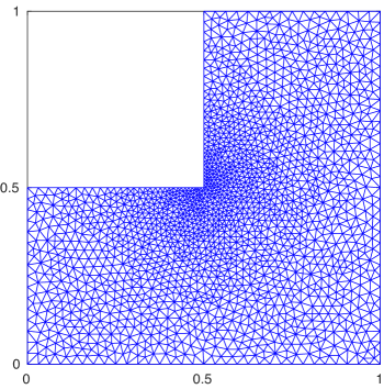
Figure 1: A non-uniform mesh for the L-shaped domain $\Omega=(0,1)^{2}\backslash([0,0.5]\times[0.5,1])$. The number of triangular elements is 3754. The mesh size around the non-convex corner is about a quarter of the other corners.

Remark 7.2

Solutions of (15) on the L-shaped domain may lose $H^{2}$-regularity due to the re-entrant corner at $(x,y)=(0.5,0.5)$. Therefore, approximate solutions constructed with only a finite element basis may not lead to sufficiently small residuals. We can obtain smaller residuals by constructing approximates solutions with the sum of finite element basis functions and a singular function of the form $r^{\frac{2}{3}}\sin\left(\frac{2}{3}\theta\right)$, where $(r,\theta)$ is a polar coordinate system centered at the re-entrant corner. In kobayashi2009constructive , a priori error estimates for such a singular function are discussed. We also quote (nakaoplumwatanabe2019numerical, , Example 7.7), an example of application to nonlinear elliptic problems. In this paper, we do not use the above singular function, but instead make the size of meshes around $(x,y)=(0.5,0.5)$ smaller than others to reduce residuals $($again, see, Fig. 1$)$. Once an $H^{1}_{0}$-error estimation of a solution is obtained, even if it is relatively rough, our method can be effective in proving the positivity of the solution.

8 Numerical Experiments

In this section, we present numerical experiments in which the positivity of solutions of (15) satisfying (4) are verified via the proposed method. All computations were implemented on a computer with 2.90 GHz Intel Xeon Platinum 8380H CPUs $\times$ 4, 3 TB RAM, and CentOS 8.2 using MATLAB 2019a with GCC Version 8.3.1. All rounding errors were strictly estimated using the toolboxes INTLAB version 11 rump1999book and kv library version 0.4.49 kashiwagikv . In the tables in this section, we use the following notation:

• $M_{u}$: number of Legendre basis functions on $\Omega=(0,1)^{2}$ with respect to $x$ and $y$ for constructing approximate solution $\hat{u}\in V_{M_{u}}$ (see (44))

• $M$: number of Legendre basis functions on $\Omega=(0,1)^{2}$ with respect to $x$ and $y$ for calculating $\|F^{\prime-1}_{\hat{u}}\|_{\mathcal{L}(H^{-1},H^{1}_{0})}$ (see (44))

• $\|F^{\prime-1}_{\hat{u}}\|$: operator norm $\|F^{\prime-1}_{\hat{u}}\|_{\mathcal{L}(H^{-1},H^{1}_{0})}$ required in (42)

• $\|F(\hat{u})\|$: residual norm $\|F(\hat{u})\|_{H^{-1}}$ required in (42)

• $L$: upper bound for Lipschitz constant satisfying (43)

• $\alpha$ and $\beta$: constants required in Theorem 7.1

• $\rho$: error bound $\|u-\hat{u}\|_{H^{1}_{0}}$

• $m$: constant that determines $D(m)$; see Lemma 3.2

• $|\text{\rm supp\,}u_{-}|$: volume of support of $u_{-}$

• $\lambda_{1}(\text{\rm supp\,}u_{-})$: first eigenvalue of $-\Delta$ on interior of $\text{\rm supp\,}u_{-}$ defined by (9)

• $\mathcal{C}_{1}$ and $\mathcal{C}_{2}$: constants required in Theorem 6.5

8.1 Lane–Emden equation

As mentioned in the Introduction, positive solutions of the Lane–Emden equation with subcritical $p>1$,

$$\left\{\begin{array}[]{l l}-\Delta u=u\left|u\right|^{p-1}&\mathrm{in~{}}\Omega,\\ u=0&\mathrm{on~{}}\partial\Omega\end{array}\right.$$ (52)

have been studied from various points of view (again, see gidas1979symmetry ; lin1994uniqueness ; damascelli1999qualitative ; gladiali2011bifurcation ; de2019morse ). This equation is covered by Theorem 6.5 (see the first row in Table 4). The Lipschitz constant $L$ satisfying (43) can be estimated as

$$L\leq p(p-1)C_{p+1}^{3}\left(\|\hat{u}\|_{L^{p+1}}+C_{p+1}r\right)^{p-2},~{}~{}r=2\alpha+\delta~{}~{}{\rm for~{}small}~{}~{}\delta>0$$

via a simple calculation from the definition, where we set $r$ to be the next floating-point number after $2\alpha$. We refer to (tanaka2020numerical, , Section 4) as a numerical experiment for positive solutions of the Lane–Emden equation for $p=3,5$ on $\Omega=(0,1)^{2}$, where the volume of $D(m)$ was roughly estimated as $|D(m)|\leq|\Omega|$.

For the L-shaped domain $\Omega=(0,1)^{2}\backslash([0,0.5]\times[0.5,1])$, we constructed an approximate solution $\hat{u}\in V_{M}$ of (52) with $p=3$ using a piecewise quadratic basis, obtaining Fig. 2. Table 5 shows the verification result and confirms the positivity of the enclosed solution because $\mathcal{C}_{1}\leq\mathcal{C}_{2}$.

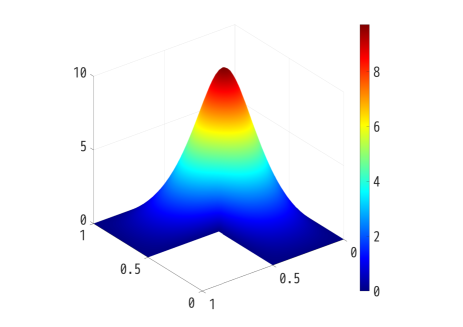
Figure 2: An approximate solution of (52) for $p=3$ on $\Omega=(0,1)^{2}\backslash([0,0.5]\times[0.5,1])$.

Table 5: Verification results for (52) for $p=3$ on $\Omega=(0,1)^{2}\backslash([0,0.5]\times[0.5,1])$. The values in rows from $\|F^{\prime-1}_{\hat{u}}\|$ to $\rho$ in row $\mathcal{C}_{1}$ represent strict upper bounds in decimal form. The value in row $|\text{\rm supp\,}u_{-}|$ represents strict lower bounds in decimal form.

$\|F^{\prime-1}_{\hat{u}}\|$	$2.03035227$
$\|\mathcal{F}(\hat{u})\|$	$4.24332160\times 10^{-2}$
$L$	$7.11899016\times 10^{-1}$
$\alpha$	$8.61543762\times 10^{-2}$
$\beta$	$1.44540578$
$\rho$	$1.03811119\times 10^{-1}$
$m$	$2^{-4}$
$|\text{\rm supp\,}u_{-}|\geq$	$8.74678937\times 10^{-2}$
$\mathcal{C}_{1}$	$3.858891\times 10^{-3}$
$\mathcal{C}_{2}$	$1$

8.2 Allen–Cahn equation and Nagumo equation

In the next example, we consider the stationary problem of the Allen–Cahn equation

$$\left\{\begin{array}[]{l l}-\Delta u=\lambda(u-u^{3})&\mathrm{in~{}}\Omega,\\ u=0&\mathrm{on~{}}\partial\Omega\end{array}\right.$$ (55)

with $\lambda>0$. This is regarded as a special case of the stationary problem of the Nagumo equation

$$\left\{\begin{array}[]{l l}-\Delta u=\lambda u(1-u)(u-a)=\lambda(-au+(1+a)u^{2}-u^{3})&\mathrm{in~{}}\Omega,\\ u=0&\mathrm{on~{}}\partial\Omega\end{array}\right.$$ (58)

with $\lambda>0$ and $0<a<1$. By applying $u=(v+1)/2$ to (58) with $a=0.5$ and adjusting the value of $\lambda$, these equations become identical. The Lipschitz constants $L$ satisfying (43) for (55) and (58) were respectively estimated as

$$L\leq 6\lambda C_{4}^{3}\left(\|\hat{u}\|_{L^{4}}+C_{4}r\right), ~{}~{}r=2\alpha+\delta~{}~{}{\rm for~{}small}~{}~{}\delta>0,$$

$$L\leq\lambda\left(2(1+a)C_{3}^{3}+6C_{4}^{3}\left(\|\hat{u}\|_{L^{4}}+C_{4}r\right)\right), ~{}~{}r=2\alpha+\delta~{}~{}{\rm for~{}small}~{}~{}\delta>0,$$

where we set $r$ to be the next floating-point number after $2\alpha$. It should be again noted that, in the previous paper tanaka2020numerical , another approach was used for (55) to confirm positivity, requiring the confirmation of the positivity of the minimal eigenvalue of a certain linearized operator around approximation $\hat{u}$. Theorem 6.5 can be uniformly applied to the nonlinearities of the form (6) (again, see Table 4).

For the square domain $\Omega=(0,1)^{2}$, we constructed approximate solutions $\hat{u}$ using a Legendre polynomial basis. For (55) ($\lambda=100$, $400$, and $1600$), we obtained Fig. 3 and the verification results in Table 6. For (58) ($\lambda=400$, $a=1/4$), we found multiple solutions displayed in Fig. 4 and the verification results in Table 7.

For the L-shaped domain $\Omega=(0,1)^{2}\backslash([0,0.5]\times[0.5,1])$, we constructed approximate solutions $\hat{u}\in V_{M}$ using a piecewise quadratic basis, obtaining Fig. 5 for (55) ($\lambda=100$) and (58) ($\lambda=180$, $a=1/64$), and the verification results in Table 8. In all cases, we confirmed $\mathcal{C}_{1}\leq\mathcal{C}_{2}$ and thus the positivity of the enclosed solutions.

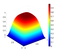
$\lambda=100$

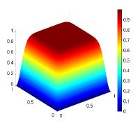
$\lambda=400$

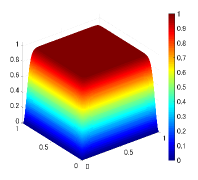
$\lambda=1600$

Figure 3: Approximate solutions of (55) on $\Omega=(0,1)^{2}$ for $\lambda=100$, $400$, and $1600$.

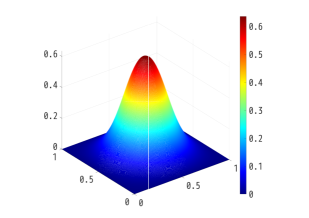
Lower solution

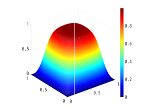
Upper solution

Figure 4: Approximations of multiple solutions of (58) on $\Omega=(0,1)^{2}$ for $\lambda=400$ and $a=1/4$.

Table 6: Verification results for (55) on $\Omega=(0,1)^{2}$ for $\lambda=100$, $400$, and $1600$. The values in rows from $\|\mathcal{F}_{\hat{u}}^{\prime-1}\|$ to $\rho$ represent strict upper bounds in decimal form. The values in rows $\lambda_{1}(\text{\rm supp\,}u_{-})$ and $\mathcal{C}_{2}$ represent strict lower bounds in decimal form.

$\lambda$	100	400	1600
$M_{u}$	40	40	60
$M$	40	40	60
$\|\mathcal{F}_{\hat{u}}^{\prime-1}\|$	$2.81346407$	$4.57367687$	$26.8136948$
$\|\mathcal{F}(\hat{u})\|$	$5.62890577\times 10^{-10}$	$2.15869521\times 10^{-6}$	$1.99428443\times 10^{-6}$
$L$	$3.05079436$	$5.02704780$	$7.57229901$
$\alpha$	$1.58367241\times 10^{-9}$	$9.87317430\times 10^{-6}$	$5.34741338\times 10^{-5}$
$\beta$	$8.58330029$	$22.9920922$	$2.03041315\times 10^{+2}$
$\rho$	$1.76247606\times 10^{-9}$	$1.78014183\times 10^{-5}$	$5.68280000\times 10^{-4}$
$m$	$2^{-4}$	$2^{-5}$	$2^{-5}$
$\lambda_{1}(\text{\rm supp\,}u_{-})\geq$	$3.24128275\times 10^{+2}$	$1.26466832\times 10^{+3}$	$2.07075690\times 10^{+3}$
$\mathcal{C}_{1}$	$0$	$0$	$0$
$\mathcal{C}_{2}\geq$	$6.914802\times 10^{-1}$	$6.837115\times 10^{-1}$	$2.273357\times 10^{-1}$

Table 7: Verification results for (58) on $\Omega=(0,1)^{2}$ for $\lambda=400$, $a=1/4$. The values in rows from $\|\mathcal{F}_{\hat{u}}^{\prime-1}\|$ to $\rho$ and in row $\mathcal{C}_{1}$ represent strict upper bounds in decimal form. The values in row $\lambda_{1}(\text{\rm supp\,}u_{-})$ represent strict lower bounds in decimal form.

Solution	Lower	Upper
$M_{u}$	40	40
$M$	40	80
$\|\mathcal{F}_{\hat{u}}^{\prime-1}\|$	$14.7881126$	$20.9590503$
$\|\mathcal{F}(\hat{u})\|$	$2.89599073\times 10^{-8}$	$7.71958696\times 10^{-8}$
$L$	$45.4341203$	$81.6094700$
$\alpha$	$4.28262367\times 10^{-7}$	$1.61795212\times 10^{-6}$
$\beta$	$6.71884883\times 10^{2}$	$1.71045699\times 10^{3}$
$\rho$	$4.28323999\times 10^{-7}$	$1.62019712\times 10^{-6}$
$m$	$2^{-4}$	$2^{-4}$
$|\text{\rm supp\,}u_{-}|\geq$	$4.99000550\times 10^{-2}$	$5.59616089\times 10^{-3}$
$\mathcal{C}_{1}$	$2.910457\times 10^{-2}$	$5.157194\times 10^{-3}$
$\mathcal{C}_{2}$	$1$	$1$

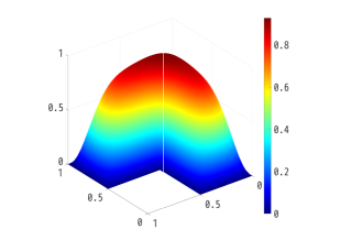
(55) with $\lambda=100$

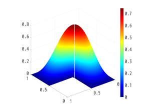
(58) with $\lambda=180$, $a=1/64$

Figure 5: Approximate solutions of (55) and (58) on $\Omega=(0,1)^{2}\backslash([0,0.5]\times[0.5,1])$.

Table 8: Verification results for (55) and (58) on $\Omega=(0,1)^{2}\backslash([0,0.5]\times[0.5,1])$. The values in rows from $\|\mathcal{F}_{\hat{u}}^{\prime-1}\|$ to $\rho$ represent strict upper bounds in decimal form. The values in row $\lambda_{1}(\text{\rm supp\,}u_{-})$ and $\mathcal{C}_{2}$ represent strict lower bounds in decimal form. The value of $\mathcal{C}_{2}$ for (58) is exactly 1.

Problem	(55) ($\lambda=100$)	(58) ($\lambda=180$, $a=1/64$)
$\|\mathcal{F}_{\hat{u}}^{\prime-1}\|$	$1.45330579$	$2.11075231$
$\|\mathcal{F}(\hat{u})\|$	$8.04913524\times 10^{-3}$	$4.93049851\times 10^{-3}$
$L$	$10.1025501$	$18.0081337$
$\alpha$	$1.1697855\times 10^{-2}$	$1.04070611\times 10^{-2}$
$\beta$	$14.6820944$	$38.0107096$
$\rho$	$1.39688500\times 10^{-2}$	$1.51162215\times 10^{-2}$
$m$	$2^{-4}$	$2^{-4}$
$\lambda_{1}(\text{\rm supp\,}u_{-})\geq$	$2.12873779\times 10^{+3}$	$8.70246701\times 10^{-2}$
$\mathcal{C}_{1}$	$0$	$1.920365\times 10^{-1}$
$\mathcal{C}_{2}$	$\geq 9.530238\times 10^{-1}$	$=1$

8.3 Elliptic equation with multiple positive solutions

For the last example, we consider the elliptic boundary value problem

$$\left\{\begin{array}[]{l l}-\Delta u=\lambda(u+Au^{2}-Bu^{3})&\mathrm{in~{}}\Omega,\\ u=0&\mathrm{on~{}}\partial\Omega,\end{array}\right.$$ (61)

given $\lambda,A,B>0$. This problem has two positive solutions when $\lambda^{*}<\lambda<\lambda_{1}(\Omega)$ for a certain $\lambda^{*}>0$ (see lions1982existence ). The Lipschitz constant $L$ for this problem can be estimated as

$$L\leq\lambda\left(2AC_{3}^{3}+6BC_{4}^{3}\left(\|\hat{u}\|_{L^{4}}+C_{4}r\right)\right),~{}~{}r=2\alpha+\delta~{}~{}{\rm for~{}small}~{}~{}\delta>0,$$

where we again set $r$ to be the next floating-point number of $2\alpha$.

To prove the positivity of solutions of (61), the previous method tanaka2020numerical requires an $L^{\infty}$-error estimation (5) and therefore is applicable to (61) only in the special cases where the solution has $H^{2}$-regularity and we can obtain an explicit bound for the embedding $H^{2}(\Omega)\hookrightarrow L^{\infty}(\Omega)$ successfully. However, the proposed method is well applicable even to (61) without assuming $H^{2}$-regularity; see again the last case in Table 4.

For the square domain $\Omega=(0,1)^{2}$, we constructed approximations $\hat{u}$ of multiple positive solutions of (61) ($\lambda=10$, $A=5$, $B=1$) using a Legendre polynomial basis, obtaining the results in Fig. 6 and Table 9. For the L-shaped domain $\Omega=(0,1)^{2}\backslash([0,0.5]\times[0.5,1])$, we constructed multiple approximate solutions $\hat{u}\in V_{M}$ of (61) ($\lambda=20$, $A=5$, $B=1$) using a piecewise quadratic basis, obtaining Fig. 7 and Table 10. Since $\mathcal{C}_{1}\leq\mathcal{C}_{2}$ holds for all cases, the positivity of the solutions are confirmed. Because solutions on the L-shaped domain have not $H^{2}$-regularity and problem (61) corresponds to the lower left case in Table 1, the previous method tanaka2020numerical cannot be applied to solutions in Fig. 7. Nevertheless, the proposed method succeeded in proving the positivity of both lower and upper solutions.

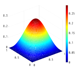
Lower solution

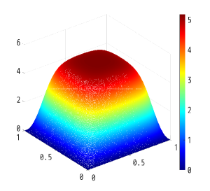
Upper solution

Figure 6: Approximations of multiple solutions of (61) on $\Omega=(0,1)^{2}$ when $\lambda=10$, $A=5$, $B=1$.

Table 9: Verification results for (61) on $\Omega=(0,1)^{2}$ when $\lambda=10$, $A=5$, $B=1$. The values in rows from $\|\mathcal{F}_{\hat{u}}^{\prime-1}\|$ to $\rho$ and in row $\mathcal{C}_{1}$ represent strict upper bounds in decimal form. The values in rows $\lambda_{1}(\text{\rm supp\,}u_{-})$ and $\mathcal{C}_{2}$ represent strict lower bounds in decimal form.

Solution	Lower	Upper
$M_{u}$	20	40
$M$	20	80
$\|\mathcal{F}_{\hat{u}}^{\prime-1}\|$	$2.11265000$	$13.7356291$
$\|\mathcal{F}(\hat{u})\|$	$2.87319486\times 10^{-9}$	$5.76722406\times 10^{-8}$
$L$	$2.52733502$	$2.77222751$
$\alpha$	$6.07005511\times 10^{-9}$	$7.92164505\times 10^{-7}$
$\beta$	$5.33937432$	$38.0782888$
$\rho$	$6.29824611\times 10^{-9}$	$1.32442923\times 10^{-6}$
$m$	$2^{-4}$	$2^{-4}$
$|\text{\rm supp\,}u_{-}|\geq$	$4.18472291\times 10^{-3}$	$4.12368775\times 10^{-3}$
$\lambda_{1}(\text{\rm supp\,}u_{-})\geq$	$47.9974691$	$1.02292545\times 10^{+2}$
$\mathcal{C}_{1}$	$1.081214\times 10^{-4}$	$7.964752\times 10^{-4}$
$\mathcal{C}_{2}\geq$	$7.916557\times 10^{-1}$	$9.902241\times 10^{-1}$

Lower solution

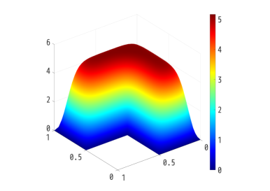
Upper solution

Figure 7: Approximations of multiple solutions of (61) on $\Omega=(0,1)^{2}\backslash([0,0.5]\times[0.5,1])$ when $\lambda=20$, $A=5$, $B=1$.

Table 10: Verification results for (61) on $\Omega=(0,1)^{2}\backslash([0,0.5]\times[0.5,1])$ when $\lambda=20$, $A=5$, $B=1$. The values in rows from $\|\mathcal{F}_{\hat{u}}^{\prime-1}\|$ to $\rho$ and in row $\mathcal{C}_{1}$ represent strict upper bounds in decimal form. The values in rows $\lambda_{1}(\text{\rm supp\,}u_{-})$ and $\mathcal{C}_{2}$ represent strict lower bounds in decimal form.

Solution	Lower	Upper
$\|\mathcal{F}_{\hat{u}}^{\prime-1}\|$	$3.93924470$	$4.17817762$
$\|\mathcal{F}(\hat{u})\|$	$1.75306001\times 10^{-3}$	$7.46385641\times 10^{-3}$
$L$	$3.78667858$	$3.83154427$
$\alpha$	$6.90573233\times 10^{-3}$	$3.11853178\times 10^{-2}$
$\beta$	$14.9166536$	$16.0088725$
$\rho$	$7.38736922\times 10^{-3}$	$6.0713451\times 10^{-2}$
$m$	$2^{-4}$	$2^{-2}$
$|\text{\rm supp\,}u_{-}|\geq$	$8.70246701\times 10^{-2}$	$8.54343721\times 10^{-2}$
$\lambda_{1}(\text{\rm supp\,}u_{-})\geq$	$56.5433134$	$6.85289494\times 10^{+4}$
$\mathcal{C}_{1}$	$7.053746\times 10^{-2}$	$1.777890\times 10^{-2}$
$\mathcal{C}_{2}\geq$	$6.462889\times 10^{-1}$	$9.997082\times 10^{-1}$

9 Conclusion

We proposed a unified a posteriori method for verifying the positivity of solutions $u$ of elliptic boundary value problem (3) while assuming $H^{1}_{0}$-error estimation (4) given some numerical approximation $\hat{u}$ and an explicit error bound $\rho$. By extending one of the approaches developed in tanaka2020numerical , we designed a unified method with wide applicability. We described the way to obtain explicit values of several constants that the proposed method requires. We also presented numerical experiments to show the effectiveness of our method for three types of nonlinearities, including those to which the previous approach is not applicable.

Appendix A Estimates of the first positive zeros of the Bessel functions

This section discusses rigorous estimates of the Bessel functions $j_{n,1}$ required to obtain the values displayed in Table 2. When $n$ is written in the form $n=k+0.5$ with an integer $k$, explicit formulas for $j_{n,1}$ can be obtained. Particularly, $j_{0.5,1}=\sqrt{2/(\pi x)}\sin x$; therefore, the first zero of this is $\pi$ (see, for example, (baricz2010generalized, , Remark 1.2) and (olver2010nist, , Section 10.16)). Moreover, we have $j_{1.5,1}=\sqrt{2/(\pi x)}\left(x^{-1}\sin x-\cos x\right)$, the zeros of which satisfy $x=\tan x$. The first zero of this function is enclosed by the function “allsol” packaged in the kv library kashiwagikv , which enables us to obtain all zeros of the function in a given compact interval. We set the initial interval as $[\pi,1.5\pi]$, in which the equation has the first zero.

When $n=0,1$, we calculated rigorous values of $j_{n,1}$ using the bisection method with computer assistance. For preparation, we first prove that there is no positive zero of $j_{0,1}$ and $j_{1,1}$ in the compact interval $[0,1]$ as follows: When $n$ is an integer, $j_{n,1}$ is given by

$$j_{n,1}(x)=\frac{1}{\pi}\int_{0}^{\pi}\cos(x\sin t-nt)dt;$$

see (olver2010nist, , Section 10.9). Let $a\geq 0$ and suppose $0\leq x\leq a$ so that $0\leq x\sin t\leq a$ ($0\leq t\leq\pi$). Let us write $A:=[0,a]$. Then, we have

$$j_{0,1}(x) =\frac{1}{\pi}\int_{0}^{\pi}\cos(x\sin t)dt\in\cos A=[\cos a,1].$$

When $a\in[0,1]\subset[0,\pi/2)$, $\cos a$ is positive, and therefore, so is $j_{0,1}$. Next, we consider $j_{1,1}$, which satisfies $j_{1,1}(0)=0$. The first derivative of $j_{1,1}$ is given by

$$\frac{d}{dx}j_{1,1}(x)=\frac{1}{\pi}\int_{0}^{\pi}\sin{t}\sin(t-x\sin t)dt.$$

Hence, we have, for $a\in[0,\pi]$,

$$\frac{d}{dx}j_{1,1}(x)\in\frac{1}{\pi}\int_{0}^{\pi}\sin{t}\sin(t-A)dt=\frac{1}{4\pi}\left(2\pi\cos A+\sin A-\sin A\right)=:B$$

For all $t\in B$, we confirm $t\geq\frac{1}{4\pi}\left(2\pi\cos a-\sin a\right)$. This value is positive when $a\in[0,1]\subset[0,\tan^{-1}(2\pi))$. Therefore, $j_{n,1}$ monotonically increases for $x\in[0,1]$.

Using bisection steps, we rigorously computed the first positive zeros of $j_{0,1}$ and $j_{1,1}$. We first found a compact interval that includes the first positive zero of $j_{n,1}$ by searching the first interval $[\underline{x},\overline{x}]:=[1+(i-1)\varepsilon/2,1+(i-1)\varepsilon/2+\varepsilon]$ ($i=1,2,\cdots$) that satisfies $j_{i,1}(\underline{x})j_{i,1}(\overline{x})<0$. Then, starting from the center of $[\underline{x},\overline{x}]$, we repeated the bisection method until the desired precision was achieved. All rounding errors were strictly estimated using kv library version 0.4.49 kashiwagikv .

References

- (1) Allen, S.M., Cahn, J.W.: A microscopic theory for antiphase boundary motion and its application to antiphase domain coarsening. Acta Metallurgica 27(6), 1085–1095 (1979)
- (2) Aubin, T.: Problèmes isopérimétriques et espaces de Sobolev. Journal of Differential Geometry 11(4), 573–598 (1976)
- (3) Baricz, Á.: Generalized Bessel functions of the first kind. Springer (2010)
- (4) Damascelli, L., Grossi, M., Pacella, F.: Qualitative properties of positive solutions of semilinear elliptic equations in symmetric domains via the maximum principle. Annales de l’Institut Henri Poincare-Nonlinear Analysis 16(5), 631–652 (1999)
- (5) Day, S., Lessard, J.P., Mischaikow, K.: Validated continuation for equilibria of pdes. SIAM Journal on Numerical Analysis 45(4), 1398–1424 (2007)
- (6) De Marchis, F., Grossi, M., Ianni, I., Pacella, F.: Morse index and uniqueness of positive solutions of the lane-emden problem in planar domains. Journal de Mathématiques Pures et Appliquées 128, 339–378 (2019)
- (7) Deuflhard, P., Heindl, G.: Affine invariant convergence theorems for Newton’s method and extensions to related methods. SIAM Journal on Numerical Analysis 16(1), 1–10 (1979)
- (8) Drábek, P.: On a maximum principle for weak solutions of some quasi-linear elliptic equations. Applied Mathematics Letters 22(10), 1567–1570 (2009)
- (9) Faber, G.: Beweis, dass unter allen homogenen Membranen von gleicher Fläche und gleicher Spannung die kreisförmige den tiefsten Grundton gibt. Sitzungsberichte der mathematisch-physikalischen Klasse der Bayerischen Akademie der Wissenschaften zu München Jahrgang 8, 169–172 (1923). https://publikationen.badw.de/en/003399311
- (10) Gidas, B., Ni, W.M., Nirenberg, L.: Symmetry and related properties via the maximum principle. Communications in Mathematical Physics 68(3), 209–243 (1979)
- (11) Gladiali, F., Grossi, M., Pacella, F., Srikanth, P.: Bifurcation and symmetry breaking for a class of semilinear elliptic equations in an annulus. Calculus of Variations and Partial Differential Equations 40(3), 295–317 (2011)
- (12) Kashiwagi, M.: kv library (2020). http://verifiedby.me/kv/
- (13) Kimura, S., Yamamoto, N.: On explicit bounds in the error for the -projection into piecewise polynomial spaces. Bulletin of informatics and cybernetics 31(2), 109–115 (1999)
- (14) Kobayashi, K.: A constructive a priori error estimation for finite element discretizations in a non-convex domain using singular functions. Japan journal of industrial and applied mathematics 26(2), 493–516 (2009)
- (15) Krahn, E.: Über eine von Rayleigh formulierte Minimaleigenschaft des Kreises. Mathematische Annalen 94, 97–100 (1925)
- (16) Krahn, E.: Über Minimaleigenschaften der Kugel in drei und mehr Dimensionen. Acta Comm. Univ. Tartu (Dorpat) A9, 1–44 (1926)
- (17) Li, P., Yau, S.T.: On the Schrödinger equation and the eigenvalue problem. Communications in Mathematical Physics 88(3), 309–318 (1983)
- (18) Lin, C.S.: Uniqueness of least energy solutions to a semilinear elliptic equation in . Manuscripta Mathematica 84(1), 13–19 (1994)
- (19) Lions, P.L.: On the existence of positive solutions of semilinear elliptic equations. SIAM review 24(4), 441–467 (1982)
- (20) Liu, X.: A framework of verified eigenvalue bounds for self-adjoint differential operators. Applied Mathematics and Computation 267, 341–355 (2015)
- (21) Liu, X., Oishi, S.: Verified eigenvalue evaluation for the Laplacian over polygonal domains of arbitrary shape. SIAM Journal on Numerical Analysis 51(3), 1634–1654 (2013)
- (22) McKean Jr, H.: Nagumo’s equation. Advances in mathematics 4(3), 209–223 (1970)
- (23) McKenna, P., Pacella, F., Plum, M., Roth, D.: A uniqueness result for a semilinear elliptic problem: A computer-assisted proof. Journal of Differential Equations 247(7), 2140–2162 (2009)
- (24) McKenna, P.J., Pacella, F., Plum, M., Roth, D.: A computer-assisted uniqueness proof for a semilinear elliptic boundary value problem. In: Inequalities and Applications 2010, pp. 31–52. Springer (2012)
- (25) Nakao, M.T., Plum, M., Watanabe, Y.: Numerical verification methods and computer-assisted proofs for partial differential equations. Springer Series in Computational Mathematics (2019)
- (26) Nakao, M.T., Watanabe, Y.: Numerical verification methods for solutions of semilinear elliptic boundary value problems. Nonlinear Theory and Its Applications, IEICE 2(1), 2–31 (2011)
- (27) Olver, F.W., Lozier, D.W., Boisvert, R.F., Clark, C.W.: NIST handbook of mathematical functions hardback and CD-ROM. Cambridge University Press (2010)
- (28) Plum, M.: Explicit -estimates and pointwise bounds for solutions of second-order elliptic boundary value problems. Journal of Mathematical Analysis and Applications 165(1), 36–61 (1992)
- (29) Plum, M.: Existence and multiplicity proofs for semilinear elliptic boundary value problems by computer assistance. Jahresbericht der Deutschen Mathematiker Vereinigung 110(1), 19–54 (2008)
- (30) Rump, S.: INTLAB - INTerval LABoratory. In: T. Csendes (ed.) Developments in Reliable Computing, pp. 77–104. Kluwer Academic Publishers, Dordrecht (1999). http://www.ti3.tuhh.de/rump/
- (31) Takayasu, A., Liu, X., Oishi, S.: Verified computations to semilinear elliptic boundary value problems on arbitrary polygonal domains. Nonlinear Theory and Its Applications, IEICE 4(1), 34–61 (2013)
- (32) Talenti, G.: Best constant in Sobolev inequality. Annali di Matematica pura ed Applicata 110(1), 353–372 (1976)
- (33) Tanaka, K.: Numerical verification method for positive solutions of elliptic problems. Journal of Computational and Applied Mathematics 370, 112647 (2020)
- (34) Tanaka, K.: A posteriori verification for the sign-change structure of solutions of elliptic partial differential equations. Japan Journal of Industrial and Applied Mathematics pp. 1–26 (2021)
- (35) Tanaka, K., Sekine, K., Mizuguchi, M., Oishi, S.: Numerical verification of positiveness for solutions to semilinear elliptic problems. JSIAM Letters 7, 73–76 (2015)
- (36) Tanaka, K., Sekine, K., Mizuguchi, M., Oishi, S.: Sharp numerical inclusion of the best constant for embedding on bounded convex domain. Journal of Computational and Applied Mathematics 311, 306–313 (2017)
- (37) Tanaka, K., Sekine, K., Oishi, S.: Numerical verification method for positivity of solutions to elliptic equations. RIMS Kôkyûroku 2037, 117–125 (2017)
- (38) Tanaka, K., Takayasu, A., Liu, X., Oishi, S.: Verified norm estimation for the inverse of linear elliptic operators using eigenvalue evaluation. Japan Journal of Industrial and Applied Mathematics 31(3), 665–679 (2014)