Identifying effects of multiple treatments in the presence of unmeasured confounding

Abstract

Identification of treatment effects in the presence of unmeasured confounding is a persistent problem in the social, biological, and medical sciences. The problem of unmeasured confounding in settings with multiple treatments is most common in statistical genetics and bioinformatics settings, where researchers have developed many successful statistical strategies without engaging deeply with the causal aspects of the problem. Recently there have been a number of attempts to bridge the gap between these statistical approaches and causal inference, but these attempts have either been shown to be flawed or have relied on fully parametric assumptions. In this paper, we propose two strategies for identifying and estimating causal effects of multiple treatments in the presence of unmeasured confounding. The auxiliary variables approach leverages variables that are not causally associated with the outcome; in the case of a univariate confounder, our method only requires one auxiliary variable, unlike existing instrumental variable methods that would require as many instruments as there are treatments. An alternative null treatments approach relies on the assumption that at least half of the confounded treatments have no causal effect on the outcome, but does not require a priori knowledge of which treatments are null. Our identification strategies do not impose parametric assumptions on the outcome model and do not rest on estimation of the confounder. This paper extends and generalizes existing work on unmeasured confounding with a single treatment and models commonly used in bioinformatics.

Keywords: Confounding; Identification; Instrumental variable; Multiple treatments.

1 Introduction

Identification of treatment effects in the presence of unmeasured confounding is a persistent problem in the social, biological, and medical sciences, where in many settings it is difficult to collect data on all possible treatment-outcome confounders. Identification means that the treatment effect of interest is uniquely determined from the joint distribution of observed variables. Without identification, statistical inference may be misleading and is of limited interest. Most of the work on unmeasured confounding by causal inference researchers focuses on settings with a single treatment, and either harnesses auxiliary variables (e.g. instruments, negative controls, or confounder proxies) to achieve point identification of causal effects, or relies on sensitivity analyses or on weak assumptions to derive bounds for the effects of interest. A large body of work from statistical genetics and computational biology is concerned with multiple treatments–for example GWAS (Genome-Wide Association Studies) with confounding by population structure and computational biology applications with confounding by batch effects. Recently, there have been a few attempts to put these approaches on solid theoretical footing and to bridge the gap between these statistical approaches and causal inference. However, these attempts either rely themselves on strong parametric models that circumvent the underlying causal structure, or have been shown to be flawed. In this paper, we propose two novel strategies for identifying causal effects of multiple treatments in the presence of unmeasured confounding without placing any parametric restrictions on the outcome model. This paper generalizes existing work on unmeasured confounding with a single treatment to the multi-treatment setting, and resolves challenges that have undermined previous proposals for dealing with multi-treatment unmeasured confounding.

1.1 Related work

For a single treatment, a variety of methods have been developed to test, adjust for, and eliminate unmeasured confounding bias. Sensitivity analysis (Cornfield et al., 1959; Rosenbaum and Rubin, 1983; Ding and Vanderweele, 2014) and bounding (Manski, 1990; Balke and Pearl, 1997; Richardson and Robins, 2014) are used to evaluate the robustness of causal inference to unmeasured confounding. For point identification of the treatment effect, the instrumental variable (IV) is an influential tool used in biomedical, epidemiological, and socioeconomic studies (Wright, 1928; Goldberger, 1972; Robins, 1994; Angrist et al., 1996; Didelez and Sheehan, 2007; Small et al., 2017). Recently, Miao et al. (2018), Shi et al. (2020), Tchetgen Tchetgen et al. (2020), Lipsitch et al. (2010), Kuroki and Pearl (2014), Ogburn and VanderWeele (2012), Flanders et al. (2017), and Wang et al. (2017) demonstrate the potential of using confounder proxy variables and negative controls for adjustment of confounding bias. For an overview of recent work in the single treatment setting, see Tchetgen Tchetgen et al. (2020) and Wang and Tchetgen Tchetgen (2018).

Similar methods can sometimes be used in settings with multiple treatments, simply treating them as a single vector-valued treatment. These approaches allow for unrestricted correlations among the treatments. However, if, as is typically the case in GWAS and computational biology settings, correlations among treatments contains useful information about the confounding, these methods cannot leverage the information. Latent variable methods leveraging the multi-treatment correlation structure have been used to estimate and control for unmeasured confounders in biological applications since the early 2000s (Alter et al., 2000; Price et al., 2006; Leek and Storey, 2007; Friguet et al., 2009; Gagnon-Bartsch and Speed, 2012; Luo and Wei, 2019). Recently, a few authors have attempted to elucidate the causal structure underlying these statistical procedures and to establish rigorous theoretical guarantees for identification, using fully parametric models. Wang et al. (2017) propose confounding adjustment approaches for the effects of a treatment on multiple outcomes under a linear factor model; by reversing the labeling of the outcome and treatments, their approaches can test but not identify the effects of multiple treatments on the outcome. Kong et al. (2021) consider a binary outcome with a univariate confounder and prove identification under a linear factor model for multiple treatments and a parametric outcome model via a meticulous analysis of the link distribution; but their approach cannot generalize to the multivariate confounder setting as we illustrate with a counterexample in the supplement. Grimmer et al. (2020), Ćevid et al. (2020), Guo et al. (2020), and Chernozhukov et al. (2017) consider linear outcome models with high-dimensional treatments that are confounded or mismeasured; in this case, identification is implied by the fact that confounding on each treatment vanishes as the number of treatments goes to infinity. In contrast, we take a fundamentally causal approach to confounding and to identification of treatment effects by allowing the outcome model to be unrestricted, the treatment-confounder distribution to lie in a more general, though not unrestricted, class of models, the number of treatments to be finite, and confounding to not vanish.

Most notably, Wang and Blei (2019) provide an intuitive justification for using latent variable methods in general multi-treatment unmeasured confounding settings; they call the justification and resulting method the “deconfounder.” Their approach uses a factor model assuming that treatments are independent conditional on the confounder to estimate the confounder, and the confounder estimate is used for adjustment of bias. However, as demonstrated in a counterexample by D’Amour (2019a) and discussed by Ogburn et al. (2019, 2020) and Imai and Jiang (2019), identification is not guaranteed for the deconfounder, i.e., the treatment effects can not be uniquely determined from the observed data even with an infinite number of data samples. Additionally, an infinite number of treatments are required for consistent estimation of the confounder, complicating finite sample inference and undermining positivity. For refinements and discussions of the deconfounder approach, see Wang and Blei (2020), D’Amour (2019a), Ogburn et al. (2020), Grimmer et al. (2020), and the commentaries (D’Amour, 2019b; Ogburn et al., 2019; Imai and Jiang, 2019; Athey et al., 2019) published alongside Wang and Blei (2019). D’Amour (2019a) suggests the proximal inference and Imai and Jiang (2019) consider the conventional instrumental variable approach to facilitate identification. However, if correlations among the multiple treatments are indicative of confounding, as the deconfounder approach assumes, neither of these two methods makes use of that correlation. Moreover, their extension to the multi-treatment setting is complicated by the fact that the proximal inference requires confounder proxies to be causally uncorrelated with any of the treatments and the instrumental variable approach requires at least as many instrumental variables as there are treatments.

1.2 Contribution

In Section 2, we review the challenges for identifying multi-treatment effects in the presence of unmeasured confounding. In Sections 3 and 4, we propose two novel approaches for the identification of causal effects of multiple treatments with unmeasured confounding: an auxiliary variables approach and a null treatments approach. Both approaches rely on two assumptions restricting the joint distribution of the unmeasured confounder and treatments. The first assumption is that the joint treatment-confounder distribution lies in a class of models that satisfy a particular equivalence property that is known to hold for many commonly-used models, e.g., many types of factor and mixture models. This assumption can accommodate other treatment-confounder models, such as mixture models, in addition to the factor models considered by Wang and Blei (2019), Kong et al. (2021), Wang et al. (2017), and Grimmer et al. (2020). The second assumption is that the treatment-confounder distribution satisfies a completeness condition that is standard in nonparametric identification problems. In addition to these two assumptions, the auxiliary variables approach leverages an auxiliary variable that does not directly affect the outcome to identify treatment effects, such as an IV or confounder proxy. In the presence of a univariate confounder, identification can be achieved with our approach even if only one auxiliary variable is available and if it is associated with only one confounded treatment. In contrast, IV approaches require as many instrumental variables as there are treatments and that all confounded treatments must be associated with the instrumental variables. The null treatments approach does not require any auxiliary variables, but instead rests on the assumption that at least half of the confounded treatments are null, without requiring knowledge of which are active and which are null. In these two approaches, identification is achieved without imposing parametric assumptions on the outcome model, although the joint treatment-confounder distribution is restricted by the equivalence and the completeness assumptions. Identification does not rest on estimation of the unmeasured confounder, and thus works with a finite number of treatments and does not run afoul of positivity. In the absence of auxiliary variables and if the null treatments assumption fails to hold, our method still constitutes a valid test of the null hypothesis of no joint treatment effect. Because identification in both approaches requires solving an integral equation, an explicit identification formula is not available for unrestricted outcome models. However, we describe some estimation strategies in Section 5. In simulations in Section 6, the proposed approaches perform well with little bias and appropriate coverage rates. In a data example about mouse obesity in Section 7, we apply the approaches to detect genes possibly causing mouse obesity, which reinforces previous findings by taking unmeasured confounding into account. Section 8 concludes with a brief mention of some potential extensions of our approaches. Proofs and further discussions are relegated to the supplement.

2 Preliminaries and challenges to identification

Throughout the paper, we let $X=(X_{1},\ldots,X_{p})^{\mathrm{\scriptscriptstyle T}}$ denote a vector of $p$ treatments and $Y$ an outcome. We are interested in the effects of $X$ on $Y$, which may be confounded by a vector of $q$ unobserved covariates $U$. The dimension of the confounder, $q$, is assumed to be known a priori; for choice of $q$ in practice see illustrations in Sections 6–7 and the discussion in Section 8. For notational convenience, we suppress observed covariates, and all conditions and results can be viewed as conditioning on them. Hereafter, we use $\Sigma_{A}$ to denote the covariance matrix of a random vector $A$. We use ${f}$ to denote a generic probability density or mass function and ${f}(A=a\mid B=b)$ the conditional density/mass of $A$ given $B$ evaluated at $(A=a,B=b)$, and write ${f}(a\mid b)$ for simplicity. Vectors are assumed to be column vectors unless explicitly transposed. We refer to ${f}(x,u)$ as the treatment-confounder distribution and ${f}(y\mid u,x)$ the outcome model.

Let $Y(x)$ denote the potential outcome that would have been observed had the treatment $X$ been set to $x$. Treatment effects are defined by contrasts of potential outcomes between different treatment conditions, and thus we focus on identification of ${f}\{Y(x)\}$. We say that ${f}\{Y(x)\}$ is identified if and only if it is uniquely determined by the joint distribution of observed variables.

Throughout we make three standard identifying assumptions.

Assumption 1.

1. Consistency: When $X=x$, $Y=Y(x)$;

2. Ignorability: $Y(x)\mathbin{\mathchoice{\hbox to0.0pt{\hbox{\set@color$\displaystyle\perp$}\hss}\kern 3.46875pt{}\kern 3.46875pt\hbox{\set@color$\displaystyle\perp$}}{\hbox to0.0pt{\hbox{\set@color$\textstyle\perp$}\hss}\kern 3.46875pt{}\kern 3.46875pt\hbox{\set@color$\textstyle\perp$}}{\hbox to0.0pt{\hbox{\set@color$\scriptstyle\perp$}\hss}\kern 2.36812pt{}\kern 2.36812pt\hbox{\set@color$\scriptstyle\perp$}}{\hbox to0.0pt{\hbox{\set@color$\scriptscriptstyle\perp$}\hss}\kern 1.63437pt{}\kern 1.63437pt\hbox{\set@color$\scriptscriptstyle\perp$}}}X\mid U$;

3. Positivity: $0<{f}(X=x\mid U=u)<1$ for all $(x,u)$.

Consistency states that the observed outcome is a realization of the potential outcome under the treatment actually received. Ignorability, also called “exchangeability,” ensures that treatment assignments are effectively randomized conditional on $U$ and implies that $U$ suffices to control for all confounding. Positivity, also called “overlap,” ensures that for all values of $U$ all treatment values have positive probability.

If we were able to observe the confounder $U$, Assumption 1 would permit fully nonparametric identification of ${f}\{Y(x)\}$ by the back-door formula (Pearl, 1995) or the g-formula (Robins, 1986),

$${f}\{Y(x)=y\}=\int_{u}{f}(y\mid u,x){f}(u)du.$$ (1)

But when $U$ is not observed, all information contained in the observed data is captured by ${f}(y,x)$, from which one cannot uniquely determine the joint distribution ${f}(y,x,u)$. To be specific, one has to solve for ${f}(x,u)$ and ${f}(y\mid u,x)$ from

$${f}(x) = \int_{u}{f}(x,u)du,$$ (2)

$${f}(y\mid x) = \int_{u}{f}(y\mid u,x){f}(u\mid x)du.$$ (3)

However, ${f}(x,u)$ cannot be uniquely determined from (2), even if, as is common practice, a factor model is imposed on ${f}(x,u)$; see D’Amour (2019a) for a counterexample. Furthermore, even if ${f}(x,u)$ is known, the outcome model ${f}(y\mid u,x)$ cannot be identified; D’Amour (2019a) points out that lack of identification of ${f}(y\mid u,x)$ is due to the unknown copula of ${f}(y\mid x)$ and ${f}(u\mid x)$. Here we note that identifying ${f}(y\mid u,x)$ given ${f}(u\mid x)$ is equivalent to solving the integral equation (3), but the solution is not unique without extra assumptions. As a result, one cannot identify the true joint distribution ${f}(y,x,u)$ that is essential for the g-formula (1). We call a joint distribution $\tilde{f}(y,x,u)$ admissible if it conforms to the observed data distribution ${f}(y,x)$, i.e., ${f}(y,x)=\int_{u}\tilde{f}(y,x,u)du$. The counterexample by D’Amour (2019a) also shows that different admissible joint distributions result in different potential outcome distributions, i.e., the potential outcome distribution is not identified without additional assumptions. Some previous approaches have estimated $U$ directly with a deterministic function of $X$, but this controverts the positivity assumption and requires an infinite number of treatments in order to consistently estimate $U$. Furthermore, Grimmer et al. (2020) show that in these settings the effect of $X$ on $Y$ is asymptotically unconfounded and a naive regression of $Y$ on $X$ weakly dominates these more involved approaches.

3 Identification with auxiliary variables

3.1 The auxiliary variables assumption

Suppose we have available a vector of auxiliary variables $Z$, then the observed data distribution is captured by ${f}(x,y,z)$, from which we aim to identify the potential outcome distribution ${f}\{Y(x)\}$. Let ${f}(x,u\mid z;\alpha)$ denote a model for the treatment-confounder distribution indexed by a possibly infinite-dimensional parameter $\alpha$, and ${f}(x\mid z;\alpha)$ the resulting marginal distribution. Given ${f}(x\mid z;\alpha)$, we let ${f}(x,u\mid z;\tilde{\alpha})$ denote an arbitrary admissible joint distribution such that ${f}(x\mid z;\alpha)=\int_{u}{f}(x,u\mid z;\tilde{\alpha})du$, and write $\tilde{f}(x,u\mid z)={f}(x,u\mid z;\tilde{\alpha})$ for short. Our identification strategy rests on the following assumption.

Assumption 2.

1. Exclusion restriction: $Z\mathbin{\mathchoice{\hbox to0.0pt{\hbox{\set@color$\displaystyle\perp$}\hss}\kern 3.46875pt{}\kern 3.46875pt\hbox{\set@color$\displaystyle\perp$}}{\hbox to0.0pt{\hbox{\set@color$\textstyle\perp$}\hss}\kern 3.46875pt{}\kern 3.46875pt\hbox{\set@color$\textstyle\perp$}}{\hbox to0.0pt{\hbox{\set@color$\scriptstyle\perp$}\hss}\kern 2.36812pt{}\kern 2.36812pt\hbox{\set@color$\scriptstyle\perp$}}{\hbox to0.0pt{\hbox{\set@color$\scriptscriptstyle\perp$}\hss}\kern 1.63437pt{}\kern 1.63437pt\hbox{\set@color$\scriptscriptstyle\perp$}}}Y\mid(X,U)$;

2. Equivalence: for any $\alpha$, any $\tilde{f}(x,u\mid z)$ that solves ${f}(x\mid z;\alpha)=\int_{u}\tilde{f}(x,u\mid z)du$ can be written as $\tilde{f}(x,u\mid z)={f}\{X=x,V(U)=u\mid z;\alpha\}$ for some invertible but not necessarily known function $V$;

3. Completeness: for any $\alpha$, ${f}(u\mid x,z;\alpha)$ is complete in $z$, i.e., for any fixed $x$ and square-integrable function $g$, $E\{g(U)\mid X=x,Z;\alpha\}=0$ almost surely if and only if $g(U)=0$ almost surely.

The exclusion restriction characterizing auxiliary variables is the same condition invoked for the treatment-inducing confounder proxies by Miao et al. (2018) and Tchetgen Tchetgen et al. (2020); it rules out the existence of a direct causal association between the auxiliary variable and the outcome. It is satisfied by instrumental variables and confounder proxies or negative controls. Figure 1 includes two directed acyclic graph (DAG) examples that satisfy the assumption. In Section 3.3 we will illustrate the difference between our use of auxiliary variables and previous proposals.

(a) An instrumental variable

(b) A nondifferential proxy of the confounder

Figure 1: Example causal diagrams for auxiliary variables.

Equivalence is a high-level assumption stating that the treatment-confounder distribution lies in a model that is identified upon a one-to-one transformation of $U$. Because ignorability holds conditional on any one-to-one transformation of $U$, this allows us to use an arbitrary admissible treatment-confounder distribution to identify the treatment effects. The equivalence property restricts the class of treatment-confounder distributions; as one example, it is not met if the dimension of confounders exceeds that of the treatments. Nonetheless, the equivalence property admits a large class of models. In particular, it allows for any factor model or mixture model that is identified, where identification in the context of these models does not imply point identification but rather identification up to a rotation (factor models) or up to label switching (mixture models). Such model assumptions are often used in bioinformatics applications where the unmeasured confounder represents population structure (GWAS) or lab batch effects (Wang et al., 2017; Wang and Blei, 2019; Luo and Wei, 2019). Identification results for factor and mixture models have been very well established (Anderson and Rubin, 1956; Kuroki and Pearl, 2014; Titterington et al., 1985; Yakowitz and Spragins, 1968). A major limitation of factor models is that they are in general not identified when there are single-treatment confounders or when there are causal relationships among the treatments (Ogburn et al., 2019). However, the equivalence assumption can accommodate models that allow for both of these features, for instance, normal mixture models (Yakowitz and Spragins, 1968); see the supplement for an example.

Completeness is a fundamental concept in statistics (see Lehman and Scheffe (1950)), and primitive conditions are readily available in the literature, including the fact that it holds for very general exponential families of distributions and for many regression models; see e.g., Newey and Powell (2003) and D’Haultfœuille (2011). Chen et al. (2014) and Andrews (2017) have shown that if $Z$ and $U$ are continuously distributed and the dimension of $Z$ is larger than that of $U$, then under a mild regularity condition the completeness condition holds generically in the sense that the set of distributions for which completeness fails has a property analogous to having zero Lebesgue measure. By appealing to such results, completeness holds in a large class of distributions and thus one may argue that it is commonly satisfied. The role of completeness in this paper is analogous to its wide use in a variety of nonparametric and semiparametric identification problems, for instance, in IV regression (Newey and Powell, 2003), IV quantile regression (Chernozhukov and Hansen, 2005), measurement error problem (Hu and Schennach, 2008), missing data (Miao and Tchetgen Tchetgen, 2016; D’Haultfœuille, 2010), and proximal inference (Miao et al., 2018). Our completeness assumption means that, conditional on $X$, any variability in $U$ is captured by variability in $Z$, analogous to the relevance condition in the instrumental variable identification. It is easiest understood in the categorical case. For the binary confounder case, completeness holds if $U$ and $Z$ are correlated within each level of $X$. When both $U$ and $Z$ have $k$ levels, completeness means that the matrix $[{f}(u_{i}\mid x,z_{j})]_{k\times k}$ consisting of the conditional probabilities is invertible. This is stronger than dependence of $Z$ and $U$ given $X$. Roughly speaking, dependence reveals that variability in $U$ is accompanied by variability in $Z$, and completeness reinforces that any infinitesimal variability in $U$ is accompanied by variability in $Z$. As a consequence, completeness in general fails if the number of levels or dimension of $Z$ is smaller than that of $U$ or $Z$ is a coarsening of $U$. In practice, completeness is more plausible if practitioners measure a rich set of potential auxiliary variables for the purpose of confounding adjustment. In the usual case that the dimension of $U$ is much smaller than that of $X$, the dimension of $Z$ can also be small. Completeness can be checked in specific models, for instance, in the categorical case. However, Canay et al. (2013) show that for unrestricted models the completeness condition is in fact untestable. In the supplement, we further elaborate the discussion on completeness and provide both positive and negative examples to facilitate its interpretation and use in practice.

Proposition 1 formalizes the equivalence and completeness conditions for the linear factor model that is widely used in GWAS and computational biology applications.

Proposition 1.

Consider a factor model $X=\alpha U+\eta Z+\varepsilon$ for a vector of $p$ observed variables $X$, $q$ unobserved confounders $U$, and $r(\geq q)$ instrumental variables $Z$ such that $Z\mathbin{\mathchoice{\hbox to0.0pt{\hbox{\set@color$\displaystyle\perp$}\hss}\kern 3.46875pt{}\kern 3.46875pt\hbox{\set@color$\displaystyle\perp$}}{\hbox to0.0pt{\hbox{\set@color$\textstyle\perp$}\hss}\kern 3.46875pt{}\kern 3.46875pt\hbox{\set@color$\textstyle\perp$}}{\hbox to0.0pt{\hbox{\set@color$\scriptstyle\perp$}\hss}\kern 2.36812pt{}\kern 2.36812pt\hbox{\set@color$\scriptstyle\perp$}}{\hbox to0.0pt{\hbox{\set@color$\scriptscriptstyle\perp$}\hss}\kern 1.63437pt{}\kern 1.63437pt\hbox{\set@color$\scriptscriptstyle\perp$}}}U\mathbin{\mathchoice{\hbox to0.0pt{\hbox{\set@color$\displaystyle\perp$}\hss}\kern 3.46875pt{}\kern 3.46875pt\hbox{\set@color$\displaystyle\perp$}}{\hbox to0.0pt{\hbox{\set@color$\textstyle\perp$}\hss}\kern 3.46875pt{}\kern 3.46875pt\hbox{\set@color$\textstyle\perp$}}{\hbox to0.0pt{\hbox{\set@color$\scriptstyle\perp$}\hss}\kern 2.36812pt{}\kern 2.36812pt\hbox{\set@color$\scriptstyle\perp$}}{\hbox to0.0pt{\hbox{\set@color$\scriptscriptstyle\perp$}\hss}\kern 1.63437pt{}\kern 1.63437pt\hbox{\set@color$\scriptscriptstyle\perp$}}}\varepsilon$. Without loss of generality we let $E(U)=0$, $\Sigma_{U}=I_{q}$, $E(\varepsilon)=0$, and $\Sigma_{\varepsilon}$ be diagonal. Assuming there remain two disjoint submatrices of rank $q$ after deleting any row of $\alpha$, we have that

• $\alpha\alpha^{\mathrm{\scriptscriptstyle T}}$ and $\Sigma_{\varepsilon}$ are uniquely determined from $\Sigma_{X-\eta Z}=\alpha\alpha^{\mathrm{\scriptscriptstyle T}}+\Sigma_{\varepsilon}$, and any admissible value for $\alpha$ can be written as $\tilde{\alpha}=\alpha R$ with $R$ an arbitrary $q\times q$ orthogonal matrix;

• if the components of $\varepsilon$ are mutually independent and the joint characteristic function of $X$ does not vanish, then any admissible joint distribution can be written as $\tilde{f}(x,u\mid z)={f}(X=x,R^{\mathrm{\scriptscriptstyle T}}U=u\mid Z=z;\alpha)$ with $R$ an arbitrary $q\times q$ orthogonal matrix;

• if $U,Z$, and $\varepsilon^{\mathrm{\scriptscriptstyle T}}$ are normal variables and $\eta^{\mathrm{\scriptscriptstyle T}}\gamma$ has full rank of $q$, then ${f}(u\mid x,z)\thicksim N(\gamma^{\mathrm{\scriptscriptstyle T}}x-\gamma^{\mathrm{\scriptscriptstyle T}}\eta z,\Sigma)$ and is complete in $z$, where $\gamma=(\Sigma_{X-\eta Z})^{-1}\alpha$, $\Sigma=I_{q}-\alpha^{\mathrm{\scriptscriptstyle T}}(\Sigma_{X-\eta Z})^{-1}\alpha$.

The first result follows from Anderson and Rubin (1956) by noting that $\eta$ is identified by the regression of $X$ on $Z$, the third result can be obtained from the completeness property of exponential families (Newey and Powell, 2003, Theorem 2.2), and we prove the second result in the supplement. The first two results hold without $Z$, i.e., when $\eta=0$. This proposition demonstrates that, for the linear factor model, any admissible value for $\alpha$ must be some rotation of the true value and any admissible treatment-confounder distribution must be the joint distribution of $X$ and some rotation of $U$. Proposition 1 requires that $p\geq 2q+1$ and that each confounder is correlated with at least three observed variables, and therefore implies “no single- or dual-treatment confounders.” This is stronger than the “no single-treatment confounder” assumption of Wang and Blei (2019); however, Grimmer et al. (2020) argue that in fact Wang and Blei (2019) require the much stronger assumption of “no finite-treatment confounding.”

3.2 Identification

Leveraging auxiliary variables gives the following identification result.

Theorem 1.

Under Assumptions 1 and 2, for any admissible joint distribution $\tilde{f}(x,u\mid z)$ that solves ${f}(x\mid z)=\int_{u}\tilde{f}(x,u\mid z)du$, there exists a unique solution $\tilde{f}(y\mid u,x)$ to the equation

$${f}(y\mid x,z)=\int_{u}\tilde{f}(y\mid u,x)\tilde{f}(u\mid x,z)du,$$ (4)

and the potential outcome distribution is identified by

$${f}\{Y(x)=y\}=\int_{u}\tilde{f}(y\mid u,x)\tilde{f}(u)du.$$ (5)

where $\tilde{f}(u)$ is obtained from $\tilde{f}(x,u\mid z)$ and ${f}(z)$.

Although the equivalence and completeness assumptions impose restrictions on the treatment-confounder distribution ${f}(x,u\mid z)$, the outcome model ${f}(y\mid u,x)$ is left unrestricted in the sense that the parameter space of ${f}(y\mid u,x)$ is all possible conditional densities of $Y$ given $X$ and a $q$-dimensional confounder $U$. Theorem 1 depicts three steps of the auxiliary variables approach. First we obtain an arbitrary admissible distribution $\tilde{f}(x,u\mid z)$; then by solving equation (4) we identify $\tilde{f}(y\mid u,x)$, which encodes the treatment effect within each stratum of the confounder; and finally we integrate the stratified effect to obtain the treatment effect in the population. The auxiliary variables approach does not estimate the confounder, or even a surrogate confounder, and thus dispenses with the need for an infinite number of treatments and avoids the forced positivity violations that were described by D’Amour (2019a, b) and Ogburn et al. (2020).

The auxiliary variable is indispensable in the second stage of the approach; without it one has to solve ${f}(y\mid x)=\int_{u}\tilde{f}(y\mid u,x)\tilde{f}(u\mid x)du$ for the outcome model. The solution to this equation is not unique given ${f}(y\mid x)$ and $\tilde{f}(u\mid x)$. However, by incorporating an auxiliary variable satisfying the exclusion restriction, we obtain equation (4), a Fredholm integral equation of the first kind (Kress, 1989, chapter 15). The solution of this equation is unique under the completeness condition and thus identifies the outcome model, up to an invertible transformation of the confounder. Equation (4) also offers testable implications for Assumption 2: if the equation does not have a solution, then Assumption 2 must be partially violated.

Unlike the g-formula (1), we do not identify the true outcome model ${f}(y\mid u,x)$ or the true confounder distribution ${f}(u)$, but instead we obtain $\tilde{f}(y\mid u,x)={f}\{y\mid V(U)=u,x\}$ and $\tilde{f}(x,u\mid z)={f}\{x,V(U)=u\mid z\}$ for some invertible transformation $V(U)$. Nonetheless, for any such admissible pair of outcome model and treatment-confounder distribution, we can still identify the potential outcome distribution, because ignorability holds conditional on any such transformation of $U$. The equivalence assumption guarantees that any admissible distribution $\tilde{f}(x,u\mid z)$ can be used for identifying the potential outcome distribution; we do not need to use the truth ${f}(x,u\mid z)$ and thus bypass the challenge to identifying it.

Although Theorem 1 shows that the potential outcome distribution is identified, the integral equation (4) does not admit an analytic solution in general and one has to resort to numerical methods. For instance, Chae et al. (2019) provide an estimation algorithm that is conjectured to provide a consistent estimator of the unknown function under mild conditions. Nonetheless, in certain special cases, a closed-form identification formula can be derived.

Example 1.

Suppose $p$ treatments, one confounder, one instrumental variable, and one outcome are generated as $X=\alpha U+\eta Z+\varepsilon$ and $Y=m(X,U,e)$, where $(\varepsilon^{\mathrm{\scriptscriptstyle T}},U,Z)$ is a vector of independent normal variables with mean zero, $\Sigma_{U}=1$, $m$ is unknown, and $e\mathbin{\mathchoice{\hbox to0.0pt{\hbox{\set@color$\displaystyle\perp$}\hss}\kern 3.46875pt{}\kern 3.46875pt\hbox{\set@color$\displaystyle\perp$}}{\hbox to0.0pt{\hbox{\set@color$\textstyle\perp$}\hss}\kern 3.46875pt{}\kern 3.46875pt\hbox{\set@color$\textstyle\perp$}}{\hbox to0.0pt{\hbox{\set@color$\scriptstyle\perp$}\hss}\kern 2.36812pt{}\kern 2.36812pt\hbox{\set@color$\scriptstyle\perp$}}{\hbox to0.0pt{\hbox{\set@color$\scriptscriptstyle\perp$}\hss}\kern 1.63437pt{}\kern 1.63437pt\hbox{\set@color$\scriptscriptstyle\perp$}}}(\varepsilon^{\mathrm{\scriptscriptstyle T}},U,Z)$. We require that at least three entries of $\alpha$ are nonzero and that $\eta^{\mathrm{\scriptscriptstyle T}}\gamma\neq 0$, in which case, the equivalence and completeness assumptions are met according to Proposition 1. Given an admissible value $\tilde{\alpha}$, we let $\tilde{\gamma}=(\Sigma_{X-\eta Z})^{-1}\tilde{\alpha}$, $\tilde{\sigma}^{2}=1-\tilde{\alpha}^{\mathrm{\scriptscriptstyle T}}(\Sigma_{X-\eta Z})^{-1}\tilde{\alpha}$, then $\tilde{f}(u\mid x,z)\thicksim N(\tilde{\gamma}^{\mathrm{\scriptscriptstyle T}}x-\tilde{\gamma}^{\mathrm{\scriptscriptstyle T}}\eta z,\tilde{\sigma}^{2})$ is an admissible distribution for ${f}(u\mid x,z)$. Let

$$h_{1}(t) =\int_{-\infty}^{+\infty}\exp(-{\rm i}tz)\phi(z)dz,$$

$$h_{2}(y,x,t) =-\frac{\tilde{\gamma}^{\mathrm{\scriptscriptstyle T}}\eta}{\tilde{\sigma}}\int_{-\infty}^{+\infty}\exp\left\{-{\rm i}t\frac{\tilde{\gamma}^{\mathrm{\scriptscriptstyle T}}x-\tilde{\gamma}^{\mathrm{\scriptscriptstyle T}}\eta z}{\tilde{\sigma}}\right\}{f}(y\mid x,z)dz,$$

be the Fourier transforms of the standard normal density function $\phi$ and ${f}(y\mid x,z)$ respectively, where ${\rm i}=(-1)^{1/2}$ denotes the imaginary unity. Then the solution to (4) with $\tilde{f}(u\mid x,z)$ given above is

$$\tilde{f}(y\mid x,u)=\frac{1}{2\pi}\int_{-\infty}^{+\infty}\exp\left(\frac{{\rm i}tu}{\tilde{\sigma}}\right)\frac{h_{2}(y,x,t)}{h_{1}(t)}dt,$$

and the potential outcome distribution is

$${f}\{Y(x)=y\}=\int_{-\infty}^{+\infty}\tilde{f}(y\mid u,x)\phi(u)du.$$

Detailed derivation for Example 1 is deferred to the supplement. If a linear outcome model is assumed and the structural causal parameter is of interest, then identification and estimation are simplified as we will discuss in Section 5.2. In the supplement, we include an additional example where identification rests on a confounder proxy variable.

3.3 A comparison to the conventional instrumental variable and proximal inference approaches

We briefly describe the difference between our auxiliary variables approach and the instrumental variable and negative control or proximal inference approaches. In addition to the exclusion restriction $(Z\mathbin{\mathchoice{\hbox to0.0pt{\hbox{\set@color$\displaystyle\perp$}\hss}\kern 3.46875pt{}\kern 3.46875pt\hbox{\set@color$\displaystyle\perp$}}{\hbox to0.0pt{\hbox{\set@color$\textstyle\perp$}\hss}\kern 3.46875pt{}\kern 3.46875pt\hbox{\set@color$\textstyle\perp$}}{\hbox to0.0pt{\hbox{\set@color$\scriptstyle\perp$}\hss}\kern 2.36812pt{}\kern 2.36812pt\hbox{\set@color$\scriptstyle\perp$}}{\hbox to0.0pt{\hbox{\set@color$\scriptscriptstyle\perp$}\hss}\kern 1.63437pt{}\kern 1.63437pt\hbox{\set@color$\scriptscriptstyle\perp$}}}Y\mid(X,U))$, the instrumental variable approach requires additional assumptions to achieve identification, such as an additive outcome model not allowing for interaction of the treatment and the confounder $E(Y\mid u,x)=m(x)+u$ as well as completeness in $z$ of ${f}(x\mid z)$ (Newey and Powell, 2003). Alternative strands of using IV for confounding adjustment include nonseparable outcome models (Imbens and Newey, 2009; Chernozhukov and Hansen, 2005; Wang and Tchetgen Tchetgen, 2018) and local average treatment effect models (Angrist et al., 1996; Ogburn et al., 2015). However, these two approaches typically focus on a single (or binary) treatment and we are not aware of any extensions for multiple treatments. Therefore, we compare our approaches to the additive model, which has a straightforward extension to multiple treatments. The completeness of ${f}(x\mid z)$ guarantees uniqueness of the solution to $E(Y\mid z)=\int_{x}m(x){f}(x\mid z)dx$, an integral equation identifying $m(x)$. In contrast, our approach does not rest on outcome model restrictions and hence accommodates interactions. Moreover, the completeness of ${f}(x\mid z)$ in $z$ entails at least as many instrumental variables as there are confounded treatments, and requires each confounded treatment to be correlated with at least one instrumental variable. But for our auxiliary variables approach, completeness of ${f}(u\mid x,z)$ in $z$ requires the dimension of $Z$ to be as great as that of $U$, which can be much smaller than that of the treatments. In the special case of a single confounder, completeness of ${f}(u\mid x,z)$ can be more plausibly achieved with only one auxiliary variable and with only one treatment correlated with it.

Proximal inference (Miao et al., 2018; Shi et al., 2020; Tchetgen Tchetgen et al., 2020) allows for unrestricted outcome models, but entails at least two confounder proxies $(W,Z)$ with exclusion restrictions: $W\mathbin{\mathchoice{\hbox to0.0pt{\hbox{\set@color$\displaystyle\perp$}\hss}\kern 3.46875pt{}\kern 3.46875pt\hbox{\set@color$\displaystyle\perp$}}{\hbox to0.0pt{\hbox{\set@color$\textstyle\perp$}\hss}\kern 3.46875pt{}\kern 3.46875pt\hbox{\set@color$\textstyle\perp$}}{\hbox to0.0pt{\hbox{\set@color$\scriptstyle\perp$}\hss}\kern 2.36812pt{}\kern 2.36812pt\hbox{\set@color$\scriptstyle\perp$}}{\hbox to0.0pt{\hbox{\set@color$\scriptscriptstyle\perp$}\hss}\kern 1.63437pt{}\kern 1.63437pt\hbox{\set@color$\scriptscriptstyle\perp$}}}(X,Z)\mid U$ and $Z\mathbin{\mathchoice{\hbox to0.0pt{\hbox{\set@color$\displaystyle\perp$}\hss}\kern 3.46875pt{}\kern 3.46875pt\hbox{\set@color$\displaystyle\perp$}}{\hbox to0.0pt{\hbox{\set@color$\textstyle\perp$}\hss}\kern 3.46875pt{}\kern 3.46875pt\hbox{\set@color$\textstyle\perp$}}{\hbox to0.0pt{\hbox{\set@color$\scriptstyle\perp$}\hss}\kern 2.36812pt{}\kern 2.36812pt\hbox{\set@color$\scriptstyle\perp$}}{\hbox to0.0pt{\hbox{\set@color$\scriptscriptstyle\perp$}\hss}\kern 1.63437pt{}\kern 1.63437pt\hbox{\set@color$\scriptscriptstyle\perp$}}}Y\mid(X,U)$, even in the single confounder setting. This approach additionally assumes existence of a function $h(w,y,x)$, called the confounding bridge function, such that ${f}(y\mid u,x)=\int_{w}h(w,y,x){f}(w\mid u)dw$, i.e., $h(w,y,x)$ suffices to depict the relationship between the confounding on $Y$ and $W$. The integral equation ${f}(y\mid x,z)=\int_{w}h(w,y,x){f}(w\mid x,z)dw$ is solved for the confounding bridge $h(w,y,x)$, and the potential outcome distribution is obtained by ${f}\{Y(x)=y\}=\int_{w}h(w,y,x){f}(w)dw$, where completeness of ${f}(u\mid x,z)$ in $z$ is also required for identification of ${f}\{Y(x)\}$.

A strength of these two approaches is that they leave the treatment-confounder distribution unrestricted. But when the correlation structure of multiple treatments is informative about the presence and nature of confounding, as is generally the case in GWAS and computational biology applications, our method can exploit this correlation structure to remove the confounding bias, while the conventional instrumental variable and proximal inference approaches are agnostic to the treatment-confounder distribution and therefore unable to leverage any information it contains.

4 Identification under the null treatments assumption

4.1 Identification

Without auxiliary variables, we let ${f}(x,u\mid\alpha)$ denote a model for the treatment-confounder distribution and ${f}(x;\alpha)$ the resulting marginal distribution indexed by a possibly infinite-dimensional parameter $\alpha$. Let ${\mathcal{C}}=\{i:{f}(u\mid x)\text{ varies with }x_{i}\}$ denote the indices of confounded treatments that are associated with the confounder and ${\mathcal{A}}=\{i:{f}(y\mid u,x)\text{ varies with }x_{i}\}$ the active ones that affect the outcome. A key feature of this identification strategy is that the analyst does not need to know which treatments are confounded or which are active. We make the following assumptions.

Assumption 3.

1. Null treatments: the cardinality of the intersection ${\mathcal{C}}\cap{\mathcal{A}}$ does not exceed $(|{\mathcal{C}}|-q)/2$, where $|{\mathcal{C}}|$ is the cardinality of ${\mathcal{C}}$ and must be larger than the dimension of $U$;

2. Equivalence: for any $\alpha$, any $\tilde{f}(x,u)$ that solves ${f}(x;\alpha)=\int_{u}\tilde{f}(x,u)du$ can be written as $\tilde{f}(x,u)={f}\{X=x,V(U)=u;\alpha\}$ for some invertible but not necessarily known function $V$;

3. Completeness: for any $\alpha$, ${f}(u\mid x;\alpha)$ is complete in any $q$-dimensional subvector $x_{\mathcal{S}}$ of the confounded treatments $x_{\mathcal{C}}$.

Analogous to Assumption 2, the equivalence and completeness assumptions restrict the treatment-confounder distribution, but hold for certain well-known classes of models like factor or mixture models. Under the equivalence assumption, one can identify the confounded treatments set ${\mathcal{C}}$ by using an arbitrary admissible joint distribution $\tilde{f}(x,u)$ without knowing the truth. The null treatments assumption entails that fewer than half of the confounded treatments can have causal effects on the outcome but does not require knowledge of which treatments are active. The assumption is reasonable in many empirical studies where only a few but not many of the treatments can causally affect the outcome. For example, in GWAS or analyzing electronic health record databases for off-label drugs that improve COVID-19 outcomes, one may expect that most treatments are null without knowing which are active treatments. A counterpart of the null treatments assumption was previously considered by Wang et al. (2017) in the context of effects of a treatment on multiple outcomes. They consider a linear factor model $Y=\alpha U+\beta X+\varepsilon$ for $p$ outcomes $(Y)$ and show that $\beta$ is identified if only a small proportion of its elements are nonzero. By reversing the roles of treatments and outcome, their approach can be adapted to test but not identify multi-treatment effects, because the coefficient in the regression of treatments on the outcome and the confounder is not the causal effect of interest. Another related concept is the $s$-sparsity (Kang et al., 2016) used in Mendelian randomization, which assumes that at most $s$ single nucleotide polymorphisms can directly affect the outcome of interest. In contrast, the null treatments assumption does not necessarily require the effects to be sparse and imposes no restrictions on the unconfounded treatments.

Leveraging the null treatments assumption gives the following identification result.

Theorem 2.

Under Assumptions 1 and 3, for any joint distribution $\tilde{f}(x,u)$ that solves ${f}(x)=\int_{u}\tilde{f}(x,u)du$, there exists a unique solution $\tilde{f}(y\mid u,x)$ to the equation

$${f}(y\mid x)=\int_{u}\tilde{f}(y\mid u,x)\tilde{f}(u\mid x)du,$$ (6)

and the potential outcome distribution is identified by

$${f}\{Y(x)=y\}=\int_{u}\tilde{f}(y\mid u,x)\tilde{f}(u)du.$$ (7)

This theorem states that treatment effects are identified if fewer than half of the confounded treatments can affect the outcome. The outcome model is left unrestricted except for the restriction imposed by the null treatments assumption.

Analogous to the auxiliary variables approaches, the equivalence assumption allows us to use an arbitrary admissible treatment-confounder distribution for identification, the null treatments assumption allows us to construct Fredholm integral equations of the first kind to solve for the outcome model, and the completeness assumption guarantees uniqueness of the solution. Without the null treatments assumption, the solution to (6) is not unique as we noted above.

Theorem 2 holds if we replace $q$ with an integer $s\geq q$ in Assumption 3, in which case, completeness is weakened but the null treatments assumption is strengthened. If the average treatment effect is of interest, we could define the active treatments set as ${\mathcal{A}}=\{i:E(Y\mid u,x)\text{ varies with }x_{i}\}$ and analogously identify $E\{Y(x)\}$. If a linear outcome model is assumed and the structural parameter is of interest, the identification and estimation are simplified. We demonstrate this in Section 5.3.

To illustrate, the following is a simple example where Assumption 3 holds and identification is achieved. We are not aware of any previous identification results for this setting, in particular when no parametric assumption is imposed on the outcome model.

Example 2.

Suppose $p$ treatments, one confounder, and one outcome are generated as $X=\alpha U+\varepsilon$ and $Y=m(X,U,e)$, where $(\varepsilon^{\mathrm{\scriptscriptstyle T}},U)$ is a vector of independent normal variables with mean zero, $\Sigma_{U}=1$, $m$ is unknown, and $e\mathbin{\mathchoice{\hbox to0.0pt{\hbox{\set@color$\displaystyle\perp$}\hss}\kern 3.46875pt{}\kern 3.46875pt\hbox{\set@color$\displaystyle\perp$}}{\hbox to0.0pt{\hbox{\set@color$\textstyle\perp$}\hss}\kern 3.46875pt{}\kern 3.46875pt\hbox{\set@color$\textstyle\perp$}}{\hbox to0.0pt{\hbox{\set@color$\scriptstyle\perp$}\hss}\kern 2.36812pt{}\kern 2.36812pt\hbox{\set@color$\scriptstyle\perp$}}{\hbox to0.0pt{\hbox{\set@color$\scriptscriptstyle\perp$}\hss}\kern 1.63437pt{}\kern 1.63437pt\hbox{\set@color$\scriptscriptstyle\perp$}}}(\varepsilon,U)$. Suppose the entries of $\alpha$ are nonzero and $m$ can depend on at most $(p-1)/2$ treatments, but we do not know which ones. In this setting, ${f}(u\mid x)\thicksim N(\gamma^{\mathrm{\scriptscriptstyle T}}x,\sigma^{2})$ with $\gamma=\Sigma_{X}^{-1}\alpha$ and $\sigma^{2}=1-\alpha^{\mathrm{\scriptscriptstyle T}}\Sigma_{X}^{-1}\alpha$. Because the entries of $\alpha$ are nonzero, the equivalence assumption is met (Proposition 1 with $\eta=0$) and all entries of $\gamma$ must be nonzero (lemma 2 in the supplement); thus, ${f}(u\mid x)$ is complete in each treatment. As a result, the potential outcome distributions and treatment effects are identified.

The null treatments approach proceeds by first obtaining an admissible $\tilde{f}(x,u)$, then finding the solution to (6), and finally calculating ${f}\{Y(x)\}$ from (7). Equation (6) cannot be solved directly as we do not know which treatments are null. As an informal, heuristic intuition for how this identification strategy works in this example, note that, if we knew the identity of any one of the null treatments we could treat it as an auxiliary variable and apply the auxiliary variables approach. In the absence of such knowledge we can imagine using each $X$ as an auxiliary variable; under the null treatments assumption more than half of the $X$’s must give the same, correct solution to (6). We describe a constructive method that formalizes this idea.

Let $x_{\mathcal{S}}$ denote an arbitrary $q$-dimensional subvector of $x_{\mathcal{C}}$ and $x_{\bar{\mathcal{S}}}$ the rest components of $x$ except for $x_{\mathcal{S}}$. Given $\tilde{f}(x,u)$ and ${f}(y\mid x)$, we solve

$${f}(y\mid x)=\int_{u}\tilde{f}(y\mid u,x_{\bar{\mathcal{S}}})\tilde{f}(u\mid x_{\mathcal{S}},x_{\bar{\mathcal{S}}})du,$$ (8)

for $\tilde{f}(y\mid u,x_{\bar{\mathcal{S}}})$ for all choices of $x_{\mathcal{S}}$.

Proposition 2.

Under Assumptions 1 and 3, for any choice for $x_{\mathcal{S}}$, if the solution to (8) exists and depends on at most $(|{\mathcal{C}}|-q)/2$ ones of the confounded treatments, then it must solve (6).

4.2 Hypothesis testing without auxiliary variables and null treatments assumptions

An immediate extension of the null treatments approach provides a test of the sharp null hypothesis of no joint effects, which requires neither auxiliary variables nor the null treatments assumption. The sharp null hypothesis is $\mathbb{H}_{0}:{f}(y\mid u,x)={f}(y\mid u)$ for all $x$.

Proposition 3.

Under Assumption 1 and (ii)–(iii) of Assumption 3 and given an admissible joint distribution $\tilde{f}(x,u)$, if the null hypothesis $\mathbb{H}_{0}$ is correct, then for any $q$-dimensional subvector $x_{\mathcal{S}}$ of the confounded treatments $x_{\mathcal{C}}$, the solution to the following equation exists and is unique,

$${f}(y\mid x)=\int_{u}\tilde{f}(y\mid u,x_{\bar{\mathcal{S}}})\tilde{f}(u\mid x_{{\mathcal{S}}},x_{\bar{\mathcal{S}}})du,$$ (9)

and the solution must satisfy the following equality,

$${f}(y)=\int_{u}\tilde{f}(y\mid u,x_{\bar{\mathcal{S}}})\tilde{f}(u)du.$$ (10)

This result allows us to construct valid hypothesis tests even in the absence of auxiliary variables or a commitment to the null treatments assumption. Under Assumption 1 and (ii)–(iii) of Assumption 3, evidence against the existence of the solution to (9) or against the equality (10) is evidence against $\mathbb{H}_{0}$. The proof is immediate by noting that, under the null hypothesis $\mathbb{H}_{0}$, the null treatments assumption is trivially satisfied. Thus, if $\mathbb{H}_{0}$ is correct, the solution to (9) does not depend $x$, and the right hand side of (10) identifying the potential outcome distribution ${f}\{Y(x)=y\}$ must be equal to the observed outcome distribution ${f}(Y=y)$.

5 Estimation

5.1 General estimation strategies

In this section we adhere to a common principle of causal inference, and indeed statistics more broadly, that is nicely summed up by Cox and Donnelly (2011) (via Imai and Jiang, 2019):

If an issue can be addressed nonparametrically then it will often be better to tackle it parametrically; however, if it cannot be resolved nonparametrically then it is usually dangerous to resolve it parametrically. (p. 96)

Having proven identification without recourse to parametric outcome models, we will see that estimation does, in fact, require them. This is similar to myriad other causal inference problems, where nonparametric identification is commonly followed by estimation via parametric or sometimes semiparametric models. One key difference is that, in the absence of parametric assumptions, there is no closed-form identifying expression for treatment effects in this setting, because in general there is no closed-form solution to the integral equations that are involved in identification. We first describe an estimation procedure in full generality and then introduce some choices of parametric outcome models that make it feasible in practice.

Theorem 1 points to the following auxiliary variables algorithm for estimation of ${f}\{Y(x)\}$.

The auxiliary variables algorithm:

• Obtain an arbitrary admissible joint distribution $\tilde{f}(x,u,z)$.

• Use the estimate from Step 1, along with an estimate of ${f}(y\mid x,z)$, to solve Equation (4) for an estimate of $\tilde{f}(y\mid u,x)$.

• Plug the estimate of $\tilde{f}(y\mid u,x)$ from Step 2 and the estimate of $\tilde{f}(u)$ derived from $\tilde{f}(u,x,z)$ into Equation (5) to estimate ${f}\{Y(x)\}$.

Theorem 2 points to the null treatments algorithm with a similar set of steps for estimation of $f\{Y(x)\}$.

The null treatments algorithm:

• Obtain an arbitrary admissible joint distribution $\tilde{f}(x,u)$.

• Use the estimate of $\tilde{f}(u\mid x)$ from Step 1, along with an estimate of ${f}(y\mid x)$, to solve Equation (6) for an estimate of $\tilde{f}(y\mid u,x)$. The constructive method described in Proposition 2 can be implemented to solve (6).

• Plug the estimate of $\tilde{f}(u)$ from Step 1 and $\tilde{f}(y\mid u,x)$ from Step 2 into Equation (7) to estimate ${f}\{Y(x)\}$.

Steps Aux-1 and Null-1 require only the equivalence assumption, which places nontrivial restrictions on the treatment-confounder distribution. To estimate $\tilde{f}(x,u)$, one needs to correctly specify a treatment-confounder model that meets the equivalence assumption, such as a factor or mixture model. Under standard factor or mixture models, estimation of $\tilde{f}(x,u)$ is well established, and we refer to the large existing body of literature for estimation techniques and properties (Anderson and Rubin, 1956; Kim and Mueller, 1978; Titterington et al., 1985). Note that, crucially, Step 1 estimates the distribution of $U$ (joint with $X$), but does not estimate $U$ itself. This is advantageous as it does not require infinite number of treatments and engender the resulting positivity problems.

Steps Aux-2 and Null-2 involve, first, estimating ${f}(y\mid x)$ or ${f}(y\mid x,z)$, which can be done parametrically or nonparametrically using standard density estimation techniques. More challenging is the second step, solving integral equations (4) and (6), which do not admit analytic solutions in general. These equations are of the form of Fredholm integral equations of the first kind (Kress, 1989, chapter 15). This kind of equation is known to be ill-posed due to noncontinuity of the solution and difficulty of computation. In the contexts of nonparametric instrumental variable regression, regularization methods have been established to solve the equation and we refer to Newey and Powell (2003); Carrasco et al. (2007) for a broad view of this problem. Numerical solution to such equations is an active area of mathematical and statistical research and is largely beyond the scope of this paper. However, we note that Chae et al. (2019) provide R code for a numerical method that is conjectured to provide a consistent estimator of the unknown function under mild conditions. In the next subsections, we describe modeling assumptions under which the integral equation can be avoided altogether.

Steps Aux-3 and Null-3 are essentially applications of the g-formula; estimation of this integral is standard in causal inference problems.

Below we provide two examples of how parametric models–in this case linear–can obviate the need to solve integral equations, permit estimation using standard software, and admit consistent estimators.

5.2 The auxiliary variables approach with linear models

Consider the following model for a $p$-dimensional treatment $X$, a $q$-dimensional confounder $U$, and an $r$-dimensional instrumental variable $Z$, with $p\geq 2q+1$ and $r\geq q$:

$$X=\alpha U+\eta Z+\varepsilon,\quad\Sigma_{U}=I_{q},\quad E(U)=0,\quad U\mathbin{\mathchoice{\hbox to0.0pt{\hbox{\set@color$\displaystyle\perp$}\hss}\kern 3.46875pt{}\kern 3.46875pt\hbox{\set@color$\displaystyle\perp$}}{\hbox to0.0pt{\hbox{\set@color$\textstyle\perp$}\hss}\kern 3.46875pt{}\kern 3.46875pt\hbox{\set@color$\textstyle\perp$}}{\hbox to0.0pt{\hbox{\set@color$\scriptstyle\perp$}\hss}\kern 2.36812pt{}\kern 2.36812pt\hbox{\set@color$\scriptstyle\perp$}}{\hbox to0.0pt{\hbox{\set@color$\scriptscriptstyle\perp$}\hss}\kern 1.63437pt{}\kern 1.63437pt\hbox{\set@color$\scriptscriptstyle\perp$}}}Z\mathbin{\mathchoice{\hbox to0.0pt{\hbox{\set@color$\displaystyle\perp$}\hss}\kern 3.46875pt{}\kern 3.46875pt\hbox{\set@color$\displaystyle\perp$}}{\hbox to0.0pt{\hbox{\set@color$\textstyle\perp$}\hss}\kern 3.46875pt{}\kern 3.46875pt\hbox{\set@color$\textstyle\perp$}}{\hbox to0.0pt{\hbox{\set@color$\scriptstyle\perp$}\hss}\kern 2.36812pt{}\kern 2.36812pt\hbox{\set@color$\scriptstyle\perp$}}{\hbox to0.0pt{\hbox{\set@color$\scriptscriptstyle\perp$}\hss}\kern 1.63437pt{}\kern 1.63437pt\hbox{\set@color$\scriptscriptstyle\perp$}}}\varepsilon,\quad\Sigma_{\varepsilon}\text{ diagonal,}$$ (11)

$$\text{there remain two disjoint submatrices of rank $q$ after deleting any row of $\alpha$},$$ (12)

$$\text{$\eta^{\mathrm{\scriptscriptstyle T}}\gamma$ has full rank of $q$, where $\gamma=(\Sigma_{X-\eta Z})^{-1}\alpha=(\Sigma_{\varepsilon}+\alpha\alpha^{\mathrm{\scriptscriptstyle T}})^{-1}\alpha$},$$ (13)

$$E(Y\mid U,X,Z)=\beta^{\mathrm{\scriptscriptstyle T}}X+\delta^{\mathrm{\scriptscriptstyle T}}U.$$ (14)

This is the IV setting from Example 1. Intercepts are not included in the models as one can center $(X,Y,Z)$ to have mean zero. If $(\varepsilon^{\mathrm{\scriptscriptstyle T}},U,Z)$ are normally distributed, then (11)–(12) imply equivalence and (13) implies completeness in Theorem 1, and as a special case, identification and estimation of ${f}\{Y(x)\}$ follows from Theorem 1 and the auxiliary variables algorithm, respectively. However, the estimation procedure below works even when the error distributions are left unspecified, in which case (11)–(13) do not suffice for identification of ${f}\{Y(x)\}$. We additionally assume the linear outcome model (14) and focus on the structural parameter $\beta$ but not the potential outcome distribution ${f}\{Y(x)\}$. Then (11)–(13), viewed as a parallel version of Assumption 2, guarantee identification of $\beta$. Condition (13) in principle can be tested after obtaining an estimator of $\eta$ and $\gamma$. Note that, $r$ may be smaller than $p$, in which case the conventional IV estimator $\hat{\beta}_{\rm iv}=(Z^{\mathrm{\scriptscriptstyle T}}X)^{-1}Z^{\mathrm{\scriptscriptstyle T}}Y$ does not work.

Estimation of $\beta$ is parallel to the auxiliary variables algorithm. We first obtain $\hat{\eta}$ by regression of $X$ on $Z$ and obtain $\hat{\gamma}$ by factor analysis of the residuals $X-\hat{\eta}Z$. There must exist some orthogonal matrix $R$ so that $\hat{\gamma}$ converges to $\gamma R$. This corresponds to Aux-1. Let $(\xi^{X},\xi^{Z})$ denote the coefficients by regression of $Y$ on $(X,Z)$ and $(\hat{\xi}^{X},\hat{\xi}^{Z})$ be the corresponding estimator. Note that $\xi^{X}=\beta+\gamma\delta$ and $\xi^{Z}=-\eta^{\mathrm{\scriptscriptstyle T}}\gamma\delta$, therefore we solve

$$\hat{\xi}^{X}=\hat{\beta}+\hat{\gamma}\hat{\delta},\quad\hat{\xi}^{Z}=-\hat{\eta}^{\mathrm{\scriptscriptstyle T}}\hat{\gamma}\hat{\delta}$$ (15)

for $(\hat{\beta},\hat{\delta})$. This corresponds to Aux-2: estimation of ${f}(y\mid x,z)$ is replaced by a linear regression of $Y$ on $(X,Z)$ and solving the integral equation for $\tilde{f}(y\mid u,x)$ is replaced by solving linear equations for finite-dimensional parameters $(\beta,\delta)$. We finally obtain

$$\hat{\beta}=\hat{\xi}^{X}+\hat{\gamma}(\hat{\gamma}^{\mathrm{\scriptscriptstyle T}}\hat{\eta}\hat{\eta}^{\mathrm{\scriptscriptstyle T}}\hat{\gamma})^{-1}\hat{\gamma}^{\mathrm{\scriptscriptstyle T}}\hat{\eta}\hat{\xi}^{Z}.$$

In the special case that the dimension of the instrumental variable $Z$ equals that of the confounder $U$, we obtain $\hat{\beta}=\hat{\xi}^{X}+\hat{\gamma}(\hat{\eta}^{\mathrm{\scriptscriptstyle T}}\hat{\gamma})^{-1}\hat{\xi}^{Z}$. Consistency and asymptotic normality follows from that of $(\hat{\xi}^{X},\hat{\xi}^{Z},\hat{\gamma},\hat{\eta})$. Routine R software such as factanal and lm can be implemented for factor analysis and linear regression, respectively, and the variance of estimators can be bootstrapped.

5.3 The null treatments approach with linear models

Consider the linear models:

$$\begin{split}X=\alpha U+\varepsilon,\quad E(Y\mid X,U)=\beta^{\mathrm{\scriptscriptstyle T}}X+\delta^{\mathrm{\scriptscriptstyle T}}U,\\ \Sigma_{U}=I_{q},\quad E(U)=0,\quad U\mathbin{\mathchoice{\hbox to0.0pt{\hbox{\set@color$\displaystyle\perp$}\hss}\kern 3.46875pt{}\kern 3.46875pt\hbox{\set@color$\displaystyle\perp$}}{\hbox to0.0pt{\hbox{\set@color$\textstyle\perp$}\hss}\kern 3.46875pt{}\kern 3.46875pt\hbox{\set@color$\textstyle\perp$}}{\hbox to0.0pt{\hbox{\set@color$\scriptstyle\perp$}\hss}\kern 2.36812pt{}\kern 2.36812pt\hbox{\set@color$\scriptstyle\perp$}}{\hbox to0.0pt{\hbox{\set@color$\scriptscriptstyle\perp$}\hss}\kern 1.63437pt{}\kern 1.63437pt\hbox{\set@color$\scriptscriptstyle\perp$}}}\varepsilon,\quad\Sigma_{\varepsilon}\text{ diagonal,}\end{split}$$ (16)

where $U$ and $\varepsilon$ are not necessarily normally distributed. The coefficient $\beta$ encoding the average treatment effects is of interest. We let $\gamma=\Sigma_{X}^{-1}\alpha$, which denotes the coefficients of regressing $U$ on $X$. Hereafter, we use $A_{i}$ to denote the $i$th row of a matrix or a column vector $A$. Let ${\mathcal{C}}=\{i:\alpha_{i}\text{ is not a zero vector}\}$ denote the indices of confounded treatments, $|{\mathcal{C}}|$ the cardinality of ${\mathcal{C}}$, and $\gamma_{\mathcal{C}}$ the submatrix consisting of the corresponding rows of $\gamma$. We have the following result.

Theorem 3.

The parameter $\beta$ is identified under model (16) and the following assumptions:

1. at most $(|{\mathcal{C}}|-q)/2$ entries of $\beta_{\mathcal{C}}$ are nonzero;

2. after deleting any row, there remain two disjoint submatrices of $\alpha$ of full rank;

3. any submatrix of $\gamma_{\mathcal{C}}$ consisting of $q$ rows has full rank.

The identification result is not compromised if $q$ is replaced with $s\geq q$ in the conditions. If the errors are normally distributed, then conditions (i)–(iii) of Theorem 3 imply the null treatments, the equivalence and the completeness conditions in Assumption 3, respectively, and identification and estimation of ${f}\{Y(x)\}$ follows from Theorem 2 and the null treatments algorithm, respectively. The estimation procedure below works for unspecified error distributions, in which case conditions (i)–(iii) in Theorem 3 no longer suffice for identification of ${f}\{Y(x)\}$, but as a parallel version of Assumption 3 they guarantee identification of $\beta$. Condition (iii) of Theorem 3 in principle can be tested after obtaining an estimator of $\gamma$.

Estimation of $\beta$ is parallel to the null treatments algorithm. Let $\xi$ denote the coefficients by regression of $Y$ on $X$. Given $n$ independent and identically distributed samples, we first obtain $\hat{\gamma}$ by factor analysis of $X$; this corresponds to Null-1. Then we obtain $\hat{\xi}$ by regression of $Y$ on $X$, which can be viewed as a crude estimator of $\beta$ with asymptotic bias $\gamma\delta$. Note that $\xi_{\mathcal{C}}=\beta_{\mathcal{C}}+\gamma_{\mathcal{C}}\delta$ for confounded treatments, then under the null treatments assumption (i) of Theorem 3, estimation of $\hat{\delta}$ can be cast as a standard robust linear regression (Rousseeuw and Leroy, 2005) given $\hat{\xi}$ and $\hat{\gamma}$: $\hat{\gamma}_{\mathcal{C}}$ is the design matrix and $\hat{\xi}_{\mathcal{C}}$ is observations with outliers corresponding to nonzero entries of $\beta_{\mathcal{C}}$. This corresponds to Null-2, where the complexity of solving integral equations is resolved by robust linear regression. Specifically, given a $n^{1/2}$-consistent estimator $(\hat{\xi},\hat{\gamma})$, we solve

$$\hat{\delta}^{\rm lms}=\arg\min_{\delta}\text{median}\ \{(\hat{\xi}_{i}-\hat{\gamma}_{i}\delta)^{2},\ i\in\hat{\mathcal{C}}\},\quad\hat{\mathcal{C}}=\{i:||\hat{\gamma}_{i}||_{2}^{2}>\log(n)/n\},$$ (17)

which is a least median of squares estimator minimizing median of the squared errors $(\hat{\xi}_{i}-\hat{\gamma}_{i}\delta)^{2}$ among the confounded treatments consistently selected by $\hat{\mathcal{C}}$. For the robust linear regression, the least quantile of squares, least trimmed squares, and the S-estimator can also be used to solve for $\delta$, which we refer to Rousseeuw and Leroy (2005, chapter 3.4). The corresponding estimate of $\beta$ is $\hat{\beta}^{\rm lms}=\hat{\xi}-\hat{\gamma}\hat{\delta}^{\rm lms}$. In the supplement, we show consistency of $(\hat{\delta}^{\rm lms},\hat{\beta}^{\rm lms})$ under the assumptions of Theorem 3 and an additional regularity condition given $n^{1/2}$-consistency of $(\hat{\xi},\hat{\gamma})$. However, they are not necessarily asymptotically normal as we observe in numerical experiments, even if $(\hat{\xi},\hat{\gamma})$ are. Therefore, to promote asymptotic normality we use $\hat{\beta}^{\rm lms}$ as an initial value to select the null treatments and to update estimates of $\delta$ and $\beta$ as follows: obtain $\hat{\delta}$ by solving $\hat{\xi}_{i}=\hat{\gamma}_{i}\hat{\delta}$ (by OLS) that corresponds to the smallest $(|\hat{\mathcal{C}}|+q)/2$ entries of $|\hat{\beta}_{\rm lms}|$ and obtain the ultimate estimator $\hat{\beta}=\hat{\xi}-\hat{\gamma}\hat{\delta}$. Routine R software factanal and lqs can be implemented for factor analysis and robust linear regression, respectively, and the variance of the ultimate estimator can be bootstrapped.

6 Simulations

6.1 The auxiliary variables setting

We evaluate performance of the proposed methods via simulations. For the auxiliary variables setting, 2 confounders $(U)$, 6 instrumental variables $(Z)$, 6 treatments $(X)$, an outcome $(Y)$, and 2 outcome-inducing confounder proxies $(W)$ are generated as follows,

$$X=\alpha U+\eta Z+\varepsilon_{X},\quad Y=\beta^{\mathrm{\scriptscriptstyle T}}X+\delta_{Y}U+\varepsilon_{Y},\quad W=\delta_{W}U+\varepsilon_{W},$$ (18)

$$U\thicksim N(0,I_{2}),\quad Z\thicksim N(0,I_{6}),\quad\varepsilon_{X}\thicksim N(0,I_{6}),\quad\varepsilon_{Y}\thicksim N(0,1);\quad\varepsilon_{W}\thicksim N(0,I_{2});$$ (19)

$$\begin{array}[]{l}\alpha=\begin{pmatrix}0&0\\ 1&0\\ 1.5&1\\ 2&-2\\ 2.5&1\\ 2&-1\end{pmatrix},\quad\eta=\begin{pmatrix}1&0&0&0&0&0\\ 0&1&0&0&0&1\\ 0&0&1&0&0&0\\ 0&0&0&1&0&0\\ 0&0&0&0&1&0\\ 1&0&0&0&0&1\\ \end{pmatrix},\quad\beta=\begin{pmatrix}1\\ 1\\ 1\\ 1\\ 1\\ 1\\ \end{pmatrix},\quad\delta_{Y}=(1,1),\quad\delta_{W}=\begin{pmatrix}2&0\\ 0&2\\ \end{pmatrix}.\end{array}$$

Under this setting, $(X_{2},\ldots,X_{6})$ are confounded but $X_{1}$ is not. For estimation, we consider eight methods:

IV1	conventional IV approach using all six IVs;
IV2	conventional IV approach using five IVs $(Z_{1},\ldots,Z_{5})$ and treating $(X_{6},Z_{6})$ as covariates;
Aux1	the proposed auxiliary variables approach assuming two factors and using all six IVs;
Aux2	the auxiliary variables approach assuming two factors,
	using $(Z_{5},Z_{6})$ as IVs and $(Z_{1},\ldots,Z_{4})$ as covariates;
Aux3	the auxiliary variables approach with one factor, using $Z_{6}$ as an IV and $(Z_{1},\ldots,Z_{5})$ as covariates;
PI1	proximal inference using $(Z_{5},Z_{6})$ and $(W_{1},W_{2})$ as the treatment- and outcome-inducing
	confounder proxies, respectively and $(Z_{1},\ldots,Z_{4})$ as covariates;
PI2	proximal inference using $Z_{6}$ and $W_{1}$ as the treatment- and outcome-inducing confounder proxy,
	respectively and $(Z_{1},\ldots,Z_{5})$ as covariates;
OLS	ordinary least squares estimation by regression $Y$ on $X$ and $Z$.

Two stage least squares are used in the above IV or PI methods. Because Grimmer et al. (2020) have shown that the deconfounder (Wang and Blei, 2019) is asymptotically equivalent to and does not outperform OLS, we do not include a separate comparison with the deconfounder. We replicate 1000 simulations at sample size 1000 and 2000. Figure 2 summarizes bias of the estimators of each parameter. As expected, IV₁, Aux₁, Aux₂, and PI₁ perform well with little bias for estimation of all parameters, because sufficient number of IVs or confounder proxies are used in these four methods and the number of factors are correctly specified in Aux₁ and Aux₂. Note that, Aux₂ uses only two IVs while IV₁ uses all six IVs and PI₁ uses two additional confounder proxies. We also compute the bootstrap confidence interval and evaluate the coverage probability for Aux₁ and Aux₂, summarized in Table 1. The 95% bootstrap confidence interval has coverage probabilities close to the nominal level of 0.95 under a moderate sample size. When using the same set of IVs, we might expect Aux₁ to be more efficient than IV₁ as the former additionally incorporates the internal dependence structure of the treatments. However, in our simulations when the sample size is increased to 10000, we observe that Aux₁ has a larger mean squared error than IV₁ for estimation of $(\beta_{3},\beta_{5})$ and Aux₁ has a larger mean squared error than Aux₂ for estimation of $\beta_{5}$. It can also be seen from the boxplots of the bias in Figure 2. This may be because the proposed auxiliary variables estimation is not efficient. Therefore, in the future it is of great interest to theoretically establish the semiparametric efficiency bound and the efficient estimator under the auxiliary variables assumption and compare to other competing methods.

In contrast, IV₂ fails to consistently estimate $\beta_{6}$ because the corresponding IV ($Z_{6}$) is not correctly used but treated as a covariate, but surprisingly, IV₂ is also biased for estimation of $\beta_{1}$ that is not confounded and can be estimated very well by all the other methods. Likewise, PI₂ is biased for estimation of $(\beta_{2},\ldots,\beta_{5})$ due to insufficient number of confounder proxies. Nonetheless, PI₂ has little bias for estimation of $\beta_{6}$. This is because $Z_{6}$ used in PI₂ is a valid IV for $X_{6}$ and the PI method is consistent even if the confounder proxies are inadequate, a property previously shown by Miao and Tchetgen Tchetgen (2018). Except for $\beta_{1}$, Aux₃ is biased for estimation of the confounded parameters because the number of factors and IVs are incorrectly specified. As expected, OLS is biased for estimation of all parameters except for $\beta_{1}$.

We also evaluate performance of the estimators when the IVs have a direct effect on the outcome. In this case, the outcome model is changed to $Y=\beta^{\mathrm{\scriptscriptstyle T}}X+\lambda Z+\delta_{Y}U+\varepsilon_{Y}$ with $\lambda=(0.2,\ldots,0.2,0.3)$, while the other settings of the data generating process remain the same. Figure S.1 in the supplement summarizes bias of the estimators. All estimators are biased for estimation of the confounded treatment effects, and no estimator outperforms the others in terms of bias. However, the IV estimators are also biased for estimation of $\beta_{1}$ while the other estimators have little bias.

In summary, all of conventional IV, proximal inference, and the proposed auxiliary variables approaches rely on the exclusion restriction assumption. If the exclusion restriction and the required conditions are satisfied, each of these approaches can properly address the multi-treatment confounding. The conventional IV entails at least as many IVs as treatments, otherwise it can be biased even for unconfounded treatments; proximal inference needs at least as many treatment- and outcome-inducing proxies as confounders; the proposed auxiliary variables approach does not rest on outcome-inducing confounder proxies but rests on a factor model and correct specification of the factor number. Therefore, to obtain a reliable causal conclusion in practice, we recommend implementing and comparing multiple applicable methods.

Table 1: Coverage probability of the $95\%$ bootstrap confidence interval based on Aux₁ and Aux₂

		$\beta_{1}$	$\beta_{2}$	$\beta_{3}$	$\beta_{4}$	$\beta_{5}$	$\beta_{6}$
Aux1		0.948	0.940	0.940	0.970	0.933	0.958
		0.943	0.949	0.954	0.950	0.933	0.949
Aux2		0.946	0.966	0.970	0.963	0.972	0.960
		0.942	0.959	0.958	0.953	0.950	0.942

Note: For each estimator, the first row is for sample size 1000 the second for 2000.

Figure 2: Bias of estimators when the exclusion restriction holds. White boxes are for sample size 1000 and gray ones for 2000.

6.2 The null treatments setting

We generate 2 confounders $(U)$, 8 treatments $(X)$, and an outcome $(Y)$ as follows,

$$\begin{array}[]{c}X=\alpha U+\varepsilon_{X},\quad Y=\beta^{\mathrm{\scriptscriptstyle T}}X+\delta_{Y}U+\varepsilon_{Y},\quad U\thicksim N(0,I_{2}),\quad\varepsilon_{X}\thicksim N(0,I_{6}),\quad\varepsilon_{Y}\thicksim N(0,1);\\ \alpha^{\mathrm{\scriptscriptstyle T}}=\begin{pmatrix}0&0.4&0.8&1.2&1.5&-0.4&-0.8&-1.2\\ 0&0.2&0.4&0.6&0.8&-0.5&-1.0&-1.2\end{pmatrix},\quad\delta_{Y}=(1,1).\end{array}$$

We consider two choices for $\beta$,

• Case 1: $\beta_{1}=\beta_{2}=\beta_{3}=1$, $\beta_{4}=\ldots=\beta_{8}=0$;

• Case 2: $\beta_{1}=\beta_{2}=\beta_{3}=1$, $\beta_{4}=\beta_{5}=0.2$, $\beta_{6}=\beta_{7}=\beta_{8}=0$.

Under these settings, $(X_{2},\ldots,X_{8})$ are confounded but $X_{1}$ is not; the null treatments assumption is satisfied in Case 1 as only two of the confounded treatments are active, but it is violated in Case 2 where $\beta_{4}$ and $\beta_{5}$ also have a small effect on $Y$.

For estimation, three methods are used: the null treatments estimation with correct dimension of the confounder (Null₁), the null treatments estimation with one confounder (Null₂), and OLS. Because no auxiliary variables are generated, we do not compare to IV, the auxiliary variables, or proximal inference approaches. We replicate 1000 simulations at sample size 2000 and 5000. Figures 3 and Figure S.2 (in the supplement) summarize bias of the estimators for Case 1 and Case 2, respectively. As expected, for estimation of $\beta_{1}$ that is not confounded, both OLS and the null treatments approach have little bias in both cases even if the number of confounders is not correctly specified. In Case 1 where the null treatments assumption is met, Null₁ has little bias because the number of confounders is correctly specified, and as shown in Table 2, the $95\%$ bootstrap confidence interval based on Null₁ has coverage probabilities approximate to the nominal level of $0.95$. But Null₂ is biased because the dimension of the confounder is specified to be smaller than the truth. The bias is smaller than the OLS, although this is not theoretically guaranteed. If the dimension of the confounder is larger than the truth, the factor analysis fails and so does the null treatments estimation. In Case 2, the null treatments assumption is violated because more than half of the confounded treatments are active. In this case, the null treatments estimation is in general biased for the confounded treatments; the bias could be larger or smaller than OLS. Therefore, to apply the null treatments estimation, one has to first assure that the majority of the treatments are null or very close to zero. Both the auxiliary variables and the null treatments approaches rest on correct specification of number of unmeasured confounders. If it is not known with high confidence, we refer to Bai and Ng (2002); Chen et al. (2012); Owen et al. (2016) and McLachlan et al. (2019) for the estimation methods, and we recommend assessing robustness of estimation by varying the specification in data analyses.

Table 2: Coverage probability of the $95\%$ bootstrap confidence interval for Case 1

		$\beta_{1}$	$\beta_{2}$	$\beta_{3}$	$\beta_{4}$	$\beta_{5}$	$\beta_{6}$	$\beta_{7}$	$\beta_{8}$
Null1		0.967	0.970	0.973	0.975	0.987	0.974	0.990	0.983
		0.943	0.958	0.959	0.967	0.969	0.961	0.963	0.975

Note: The first row is for sample size 2000 and the second for 5000.

Figure 3: Bias of estimators in Case 1. White boxes are for sample size 2000 and gray ones for 5000.

7 Application to a mouse obesity study

For further illustration, we reanalyze a mouse obesity dataset described by Wang et al. (2006), where the effect of gene expressions on the body weight of F2 mice is of interest. Unmeasured confounding may arise in such gene expression studies due to batch effects or unmeasured phenotypes. The data we use are collected from 227 mice, including the body weight $(Y)$, 17 gene expressions ($X$), and 5 single nucleotide polymorphisms ($Z$); see the supplement for a complete list of these variables. As previously selected by Lin et al. (2015), the 17 genes are likely to affect mouse weight and the 5 single nucleotide polymorphisms are potential instrumental variables. We further evaluate the effects of these genes on mouse weight by adopting a factor model that is widely used to characterize the unmeasured confounding in gene expression studies (Gagnon-Bartsch and Speed, 2012; Wang et al., 2017). We assume a linear outcome model and estimate the parameters with three methods: the auxiliary variables approach using single nucleotide polymorphisms as instrumental variables, the null treatments approach assuming that fewer than half of genes can affect the mouse weight, and ordinary least squares. We also compute the bootstrap confidence intervals.

Figure 4 presents the point estimates and their significance for the 17 genes, when the factor number is specified as one for the auxiliary variables and the null treatments estimation. Detailed results including point and interval estimates are relegated to the supplement. All three methods agree with positive and significant effects of Gstm2, Sirpa, and 2010002N04Rik, and a negative effect of Dscam. Additionally, the auxiliary variables estimation also indicates negative and significant effects of Igfbp2, Avpr1a, Abca8a, and Irx3; the null treatments estimation suggests a potentially positive effect of Gpld1. These results reinforce previous findings about the effects of genes on obesity. For instance, recent studies show that Igfbp2 (Insulin-like growth factor binding protein 2) protects against the development of obesity (Wheatcroft et al., 2007); Gpld1 (Phosphatidylinositol-glycan-specific phospholipase D) is associated with the change in insulin sensitivity in response to the low-fat diet (Gray et al., 2008); and Irx3 (Iroquois homebox gene 3) is associated with lifestyle changes and plays a crucial role in determining weight via energy balance (Schneeberger, 2019).

However, the significance test (Kim and Mueller, 1978, chapter IV) of the hypothesis that one factor is sufficient is rejected, indicating that either the number of factors is too small or there exists model misspecification. Figure S.3 in the supplement shows the results when the number of factors is increased to two and three. With two factors, Gstm2, 2010002N04Rik, Igfbp2, and Avpr1a remain significant in the auxiliary variables analysis, and Gstm2 and Dscam remain significant in the null treatments analysis. With three factors, all estimates in both the auxiliary variables and the null treatments analyses are no longer significant. In summary, the association between the 17 genes and mice obesity can be explained by three or more unmeasured confounders. But if there exist only one or two confounders, Gstm2, Sirpa, 2010002N04Rik, Dscam, Igfbp2, Avpr1a, Abca8a, Irx3, and Gpld1 have a potential causal association with mouse obesity, which can not be completely attributed to confounding. In future studies, it is of interest to identify the potential confounders and to use additional data to more confidently estimate effects of these 9 genes.

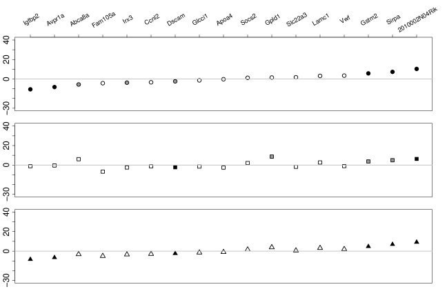
Figure 4: Effect estimates for 17 genes when one factor is used in analyses. The first panel is for the auxiliary variables estimation, the second for the null treatments estimation, and the last for ordinary least squares estimation. Black points are for significant estimates at level of $0.05$, gray ones for $0.1$, and white ones for estimates not significant at $0.1$.

8 Discussion

In this paper, we extend results that had previously been developed for the identification of treatment effects in the presence of unmeasured confounding in the single-treatment to the multi-treatment setting, and we extend the parametric approach of Wang et al. (2017) to identification of multi-treatment effects with an unrestricted outcome model. We demonstrate a novel framework using integral equations and completeness conditions to establish identification in causal inference problems.

We have assumed that the number of confounders is known, which is realistic in confounder measurement error or misclassification problems. When it is not known a priori, consistent estimation of the number of confounders has been well established by Bai and Ng (2002) under factor models and by Chen et al. (2012) under mixture models. The R software factanal provides a significance test of whether the number of factors in a factor model is sufficient to capture the full dimensionality of the data set. We also refer to Owen et al. (2016) and McLachlan et al. (2019) for a comprehensive literature review related to choosing the number of confounders in practice. We also recommend conducting a sensitivity analysis like in the simulations and the application by altering the specification of the number of confounders to assess the robustness of the substantive conclusion.

Our identification framework rests on the auxiliary variables or the null treatments assumption. These assumptions are partially testable: a heuristic approach, taking equation (4) as an example, is to check whether a solution exists. This can be achieved by obtaining a solution $\tilde{f}(y\mid u,x)$ that minimizes the mean squared error $||{f}(y\mid x,z)-\int_{u}\tilde{f}(y\mid u,x)\tilde{f}(u\mid x,z)du||^{2}$ and checking how far away the error is from zero to assess how well the solution fits the equation. This is a typical goodness-of-fit test if all models are parametric. However, in nonparametric models statistical inference for the integral equation is quite difficult and we leave the development of falsification tests for future research. Even if both the auxiliary variables and the null treatments assumptions fail to hold, we describe how to test whether treatment effects exist. The proposed estimation strategies can also be used to test whether unmeasured confounding is present, by assessing how far the proposed estimates are from the crude ones.

Our identification results lead to feasible estimation methods under parametric estimation assumptions. The proposed estimation methods, comprised of standard factor analysis, linear and robust linear regression, inherit properties from the classical theory of statistical inference; these methods work well in simulations and an application. However, statistical inference for nonparametric and semiparametric models remains to be studied. We have considered fixed dimensions of treatments and confounders, and extensions to large and high-dimensional settings are of both theoretical and practical interest.

Supplementary material

Supplementary material online includes proof of theorems and propositions, useful lemmas, discussion and examples on the completeness condition, consistency of the least median of squares estimator, discussion on identification of a parametric model for a binary outcome, details for examples, additional results for simulations and the application, and codes for reproducing the results in this article.

Online supplement to “Identifying effects of multiple treatments in the presence of unmeasured confounding”

This supplement includes

• proof of theorems and propositions, useful lemmas,

• discussion and examples on the completeness condition,

• consistency of the least median of squares estimator,

• discussion on identification of a parametric model for a binary outcome,

• details for examples, and

• additional results for simulations and the application.

S.1 Proof of propositions and theorems

S.1.1 Proof of Proposition 1

Note that $\eta$ can be identified by regression of $X$ on $Z$, then applying lemma 5.1 and theorem 5.1 of Anderson and Rubin (1956) to the factor model for the residuals,

$$X-\eta Z=\alpha U+\varepsilon,$$

we obtain (i) of Proposition 1. The third result of Proposition 1 can be obtained from the well-known completeness property of exponential families, see Theorem 2.2 of Newey and Powell (2003). Here we prove (ii), which rests on the following lemma described by Kotlarski (1967, lemma 1 and remark 5).

Lemma 1 (Kotlarski, 1967).

Let $U$, $\varepsilon_{1}$, and $\varepsilon_{2}$ be three independent $q$-dimensional real random vectors with mean zero, and let $W_{1}=U+\varepsilon_{1}$ and $W_{2}=U+\varepsilon_{2}$. If the joint characteristic function of $(W_{1},W_{2})$ does not vanish, then the distributions of $U$, $\varepsilon_{1}$, and $\varepsilon_{2}$ are uniquely determined from the joint distribution of $(W_{1},W_{2})$.

We apply Kotlarski’s lemma to prove (ii) of Proposition 1.

Proof of Proposition 1 (ii).

We denote $W=X-\eta Z=\alpha U+\varepsilon$. Note that from (i) of proposition 1, any admissible value for $\alpha$ can be written as $\tilde{\alpha}=\alpha R$ with $R$ an arbitrary $q\times q$ orthogonal matrix, we only need to prove that given $\tilde{\alpha}=\alpha R$, the joint distribution $\tilde{f}(w,u)={f}(W=w,U=u;\tilde{\alpha})$ is uniquely determined and $\tilde{f}(w,u)={f}(W=w,R^{\mathrm{\scriptscriptstyle T}}U=u;\alpha)$.

Because after deleting any row of $\alpha$ there remain two full-rank submatrices of $\alpha$, there must exist two disjoint square submatrices of $\alpha$ with full rank $q$. Note that $\tilde{\alpha}=\alpha R$, there must exist two disjoint square submatrices of $\tilde{\alpha}$ with full rank $q$, which we denote by $\tilde{\alpha}_{\mathcal{I}}$ and $\tilde{\alpha}_{\mathcal{J}}$ with ${\mathcal{I}}$ and ${\mathcal{J}}$ denoting the corresponding indices, respectively. Note that $W_{\mathcal{I}}=\tilde{\alpha}_{\mathcal{I}}V+\varepsilon_{\mathcal{I}}$ and $W_{\mathcal{J}}=\tilde{\alpha}_{\mathcal{J}}V+\varepsilon_{\mathcal{J}}$ with $V=R^{\mathrm{\scriptscriptstyle T}}U$, we have $\tilde{\alpha}_{\mathcal{I}}^{-1}W_{\mathcal{I}}=V+\tilde{\alpha}_{\mathcal{I}}^{-1}\varepsilon_{\mathcal{I}}$ and $\tilde{\alpha}_{\mathcal{J}}^{-1}W_{\mathcal{J}}=V+\tilde{\alpha}_{\mathcal{J}}^{-1}\varepsilon_{\mathcal{J}}$. According to Lemma 1, the distributions of $V$, $\tilde{\alpha}_{\mathcal{I}}^{-1}\varepsilon_{\mathcal{I}}$, and $\tilde{\alpha}_{\mathcal{J}}^{-1}\varepsilon_{\mathcal{J}}$ are uniquely determined given $\tilde{\alpha}$, and therefore, the distribution of $\varepsilon=W-\tilde{\alpha}V$ is uniquely determined. As a result, given $\tilde{\alpha}$, there is only one admissible joint distribution, which must be $\tilde{f}(w,u)={f}(W=w,R^{\mathrm{\scriptscriptstyle T}}U=u\mid\alpha)$. ∎

S.1.2 Proof of Theorem 1

Proof.

Under the equivalence (Assumption 2 (ii)), given any admissible joint distribution $\tilde{f}(x,u\mid z)$, there must exist some invertible function $V(U)$ such that $\tilde{f}(x,u\mid z)={f}\{X=x,V(U)=u\mid z\}$. Because $V(U)$ is invertible, the ignorability assumption 1 ($Y(x)\mathbin{\mathchoice{\hbox to0.0pt{\hbox{\set@color$\displaystyle\perp$}\hss}\kern 3.46875pt{}\kern 3.46875pt\hbox{\set@color$\displaystyle\perp$}}{\hbox to0.0pt{\hbox{\set@color$\textstyle\perp$}\hss}\kern 3.46875pt{}\kern 3.46875pt\hbox{\set@color$\textstyle\perp$}}{\hbox to0.0pt{\hbox{\set@color$\scriptstyle\perp$}\hss}\kern 2.36812pt{}\kern 2.36812pt\hbox{\set@color$\scriptstyle\perp$}}{\hbox to0.0pt{\hbox{\set@color$\scriptscriptstyle\perp$}\hss}\kern 1.63437pt{}\kern 1.63437pt\hbox{\set@color$\scriptscriptstyle\perp$}}}X\mid U$) implies that $Y(x)\mathbin{\mathchoice{\hbox to0.0pt{\hbox{\set@color$\displaystyle\perp$}\hss}\kern 3.46875pt{}\kern 3.46875pt\hbox{\set@color$\displaystyle\perp$}}{\hbox to0.0pt{\hbox{\set@color$\textstyle\perp$}\hss}\kern 3.46875pt{}\kern 3.46875pt\hbox{\set@color$\textstyle\perp$}}{\hbox to0.0pt{\hbox{\set@color$\scriptstyle\perp$}\hss}\kern 2.36812pt{}\kern 2.36812pt\hbox{\set@color$\scriptstyle\perp$}}{\hbox to0.0pt{\hbox{\set@color$\scriptscriptstyle\perp$}\hss}\kern 1.63437pt{}\kern 1.63437pt\hbox{\set@color$\scriptscriptstyle\perp$}}}X\mid V(U)$, the exclusion restriction $Z\mathbin{\mathchoice{\hbox to0.0pt{\hbox{\set@color$\displaystyle\perp$}\hss}\kern 3.46875pt{}\kern 3.46875pt\hbox{\set@color$\displaystyle\perp$}}{\hbox to0.0pt{\hbox{\set@color$\textstyle\perp$}\hss}\kern 3.46875pt{}\kern 3.46875pt\hbox{\set@color$\textstyle\perp$}}{\hbox to0.0pt{\hbox{\set@color$\scriptstyle\perp$}\hss}\kern 2.36812pt{}\kern 2.36812pt\hbox{\set@color$\scriptstyle\perp$}}{\hbox to0.0pt{\hbox{\set@color$\scriptscriptstyle\perp$}\hss}\kern 1.63437pt{}\kern 1.63437pt\hbox{\set@color$\scriptscriptstyle\perp$}}}Y\mid(U,X)$ implies that $Z\mathbin{\mathchoice{\hbox to0.0pt{\hbox{\set@color$\displaystyle\perp$}\hss}\kern 3.46875pt{}\kern 3.46875pt\hbox{\set@color$\displaystyle\perp$}}{\hbox to0.0pt{\hbox{\set@color$\textstyle\perp$}\hss}\kern 3.46875pt{}\kern 3.46875pt\hbox{\set@color$\textstyle\perp$}}{\hbox to0.0pt{\hbox{\set@color$\scriptstyle\perp$}\hss}\kern 2.36812pt{}\kern 2.36812pt\hbox{\set@color$\scriptstyle\perp$}}{\hbox to0.0pt{\hbox{\set@color$\scriptscriptstyle\perp$}\hss}\kern 1.63437pt{}\kern 1.63437pt\hbox{\set@color$\scriptscriptstyle\perp$}}}Y\mid\{X,V(U)\}$, and the completeness (Assumption 2 (iii)) implies that $\tilde{f}(u\mid x,z)$ is also complete in $z$. Letting $\tilde{f}(y\mid u,x)={f}\{y\mid V(U)=u,x\}$, then we have that

$${f}\{Y(x)=y\}=\int_{u}{f}(y\mid u,x){f}(u)du=\int_{u}\tilde{f}(y\mid u,x)\tilde{f}(u)du,$$ (S.1)

$${f}(y\mid x,z)=\int_{u}\tilde{f}(y\mid u,x)\tilde{f}(u\mid x,z)du,$$ (S.2)

with $\tilde{f}(u)$ and $\tilde{f}(u\mid x,z)$ derived from $\tilde{f}(x,u\mid z)$. Because $\tilde{f}(u\mid x,z)$ is complete in $z$, the solution to (S.2) is unique; this is because for any candidate solutions $\tilde{f}_{1}(y\mid u,x)$ and $\tilde{f}_{2}(y\mid u,x)$ to (S.2), we must have that $\int_{u}\{\tilde{f}_{1}(y\mid u,x)-\tilde{f}_{2}(y\mid u,x)\}\tilde{f}(u\mid x,z)=0$, which implies that $\tilde{f}_{1}(y\mid u,x)=\tilde{f}_{2}(y\mid u,x)$ by the completeness of $\tilde{f}(u\mid x,z)$ in $z$. Thus, $\tilde{f}(y\mid u,x)$ is uniquely determined from (S.2), and ${f}\{Y(x)\}$ is identified by plugging in it into (S.1). ∎

S.1.3 Proof of Theorem 2

Proof.

Under the equivalence (Assumption 3 (ii)), for any admissible joint distribution $\tilde{f}(x,u)$ we must have some invertible function $V(U)$ such that $\tilde{f}(u,x)={f}\{X=x,V(U)=u\}$. Letting ${\mathcal{C}}=\{i:{f}(u\mid x)\text{ varies with }x_{i}\}$ and $\tilde{\mathcal{C}}=\{i:\tilde{f}(u\mid x)\text{ varies with }x_{i}\}$, then we must have ${\mathcal{C}}=\tilde{\mathcal{C}}$ by noting that $\tilde{f}(u\mid x)={f}\{V(U)=u\mid x\}$, i.e., ${\mathcal{C}}$ can be identified from any admissible joint distribution $\tilde{f}(x,u)$.

Because $V(U)$ is invertible, the ignorability assumption 1 $(Y(x)\mathbin{\mathchoice{\hbox to0.0pt{\hbox{\set@color$\displaystyle\perp$}\hss}\kern 3.46875pt{}\kern 3.46875pt\hbox{\set@color$\displaystyle\perp$}}{\hbox to0.0pt{\hbox{\set@color$\textstyle\perp$}\hss}\kern 3.46875pt{}\kern 3.46875pt\hbox{\set@color$\textstyle\perp$}}{\hbox to0.0pt{\hbox{\set@color$\scriptstyle\perp$}\hss}\kern 2.36812pt{}\kern 2.36812pt\hbox{\set@color$\scriptstyle\perp$}}{\hbox to0.0pt{\hbox{\set@color$\scriptscriptstyle\perp$}\hss}\kern 1.63437pt{}\kern 1.63437pt\hbox{\set@color$\scriptscriptstyle\perp$}}}X\mid U)$ implies that $Y(x)\mathbin{\mathchoice{\hbox to0.0pt{\hbox{\set@color$\displaystyle\perp$}\hss}\kern 3.46875pt{}\kern 3.46875pt\hbox{\set@color$\displaystyle\perp$}}{\hbox to0.0pt{\hbox{\set@color$\textstyle\perp$}\hss}\kern 3.46875pt{}\kern 3.46875pt\hbox{\set@color$\textstyle\perp$}}{\hbox to0.0pt{\hbox{\set@color$\scriptstyle\perp$}\hss}\kern 2.36812pt{}\kern 2.36812pt\hbox{\set@color$\scriptstyle\perp$}}{\hbox to0.0pt{\hbox{\set@color$\scriptscriptstyle\perp$}\hss}\kern 1.63437pt{}\kern 1.63437pt\hbox{\set@color$\scriptscriptstyle\perp$}}}X\mid V(U)$, and the completeness (Assumption 3 (iii)) implies that $\tilde{f}(u\mid x)$ is also complete in $x_{\mathcal{S}}$ for any ${\mathcal{S}}\subset{\mathcal{C}}$ with cardinality $q$. Letting $\tilde{f}(y\mid u,x)={f}\{y\mid V(U)=u,x\}$, then we have that

$${f}\{Y(x)=y\}=\int_{u}{f}(y\mid u,x){f}(u)du=\int_{u}\tilde{f}(y\mid u,x)\tilde{f}(u)du,$$ (S.3)

$${f}(y\mid x)=\int_{u}\tilde{f}(y\mid u,x)\tilde{f}(u\mid x)du,$$ (S.4)

with $\tilde{f}(u)$ and $\tilde{f}(u\mid x)$ obtained from $\tilde{f}(x,u)$.

We prove that $\tilde{f}(y\mid u,x)$ is uniquely determined from (S.4) given ${f}(y\mid x)$ and $\tilde{f}(u\mid x)$ by way of contradiction. Suppose two candidate outcome models $\tilde{f}_{1}(y\mid u,x)$ and $\tilde{f}_{2}(y\mid u,x)$ satisfy (S.4), then $\int_{u}\{\tilde{f}_{1}(y\mid u,x)-\tilde{f}_{2}(y\mid u,x)\}\tilde{f}(u\mid x)=0$. Under the null treatments assumption, each of $\tilde{f}_{1}(y\mid u,x)$ and $\tilde{f}_{2}(y\mid u,x)$ can depend on only $(|{\mathcal{C}}|-q)/2$ confounded treatments, and thus the contrast $\{\tilde{f}_{1}(y\mid u,x)-\tilde{f}_{2}(y\mid u,x)\}$ can depend on at most $|{\mathcal{C}}|-q$ confounded treatments. We let $X_{\mathcal{S}}$ denote the rest $q$ confounded treatments that the contrast $\{\tilde{f}_{1}(y\mid u,x)-\tilde{f}_{2}(y\mid u,x)\}$ does not depend on, then the completeness (Assumption 3(iii)) implies that $\tilde{f}(u\mid x_{\mathcal{S}},x_{\bar{\mathcal{S}}})$ is complete in $x_{\mathcal{S}}$, and thus $\{\tilde{f}_{1}(y\mid u,x)-\tilde{f}_{2}(y\mid u,x)\}=0$ almost surely, i.e., $\tilde{f}_{1}(y\mid u,x)=\tilde{f}_{2}(y\mid u,x)$ almost surely. Therefore, the solution to (S.4) must be unique. Finally, plugging in $\tilde{f}(y\mid u,x)$ and $\tilde{f}(u)$ into (S.3) identifies the potential outcome distribution. ∎

S.1.4 Proof of Proposition 2

Proof.

We first note that the confounded treatments can be identified under the equivalence assumption, by the argument in the proof of Theorem 2. Note that the candidate solutions depending on more than $(|{\mathcal{C}}|-q)/2$ confounded treatments contradict the null treatments assumption that at most $(|{\mathcal{C}}|-q)/2$ confounded ones can affect the outcome, we only focus on solutions that depends on at most $(|{\mathcal{C}}|-q)/2$ confounded treatments.

We let $A_{\mathcal{C}}$ denotes the number of active ones of the confounded treatments. Consider a solution $\tilde{f}(y\mid u,x_{\mathcal{B}})$ that solves

$${f}(y\mid x)=\int_{u}\tilde{f}(y\mid u,x_{\mathcal{B}})\tilde{f}(u\mid x)du.$$ (S.5)

where $|\mathcal{B}\cap{\mathcal{C}}|\leq(|{\mathcal{C}}|-q)/2$, i.e., $x_{\mathcal{B}}$ includes at most $(|{\mathcal{C}}|-q)/2$ confounded treatments. Equation (S.5) is a Fredholm integral equation of the first kind with the kernel $\tilde{f}(u\mid x)$ complete in $x_{\bar{\mathcal{B}}}$, where $x_{\bar{\mathcal{B}}}$ denotes the remaining treatments of $x$ except for $x_{\mathcal{B}}$. For $x_{{\mathcal{B}}}$ that includes all active treatments, i.e., $x_{\mathcal{A}}\subset x_{\mathcal{B}}$ and $|\mathcal{B}\cap{\mathcal{C}}|=A_{\mathcal{C}}$, the solution to (S.5) exists and must be unique and equal to $\tilde{f}(y\mid u,x_{\mathcal{A}})$. For $x_{{\mathcal{B}}}$ that includes $t<A_{\mathcal{C}}$ active ones of the confounded treatments, i.e., $|\mathcal{B}\cap{\mathcal{C}}|=t<A_{\mathcal{C}}$, the solution to (S.5) does not exist. We prove this by way of contradiction.

Suppose (S.5) has a solution $\tilde{f}(y\mid u,x_{\mathcal{B}})$, then it must also satisfy the following equation

$${f}(y\mid x)=\int_{u}\tilde{f}(y\mid u,x_{\mathcal{B}}\cup x_{\mathcal{A}})\tilde{f}(u\mid x)du;$$ (S.6)

where the unknown function $\tilde{f}(y\mid u,x_{\mathcal{B}}\cup x_{\mathcal{A}})$ of $u$ is allowed to depend on all active treatments. Note that $\tilde{f}(y\mid u,x_{\mathcal{B}}\cup x_{\mathcal{A}})$ can depend on at most $(|{\mathcal{C}}|-q)/2-t$ null ones of the confounded treatments, Equation (S.6) is a Fredholm integral equation of the first kind, with the kernel $\tilde{f}(u\mid x)$ complete in $x_{\bar{\mathcal{B}}}\cap x_{\bar{\mathcal{A}}}\cap x_{\mathcal{C}}$, i.e., the remaining $q+t$ null ones of the confounded treatments. Therefore, (S.6) can be satisfied by only one function, which in fact is $\tilde{f}(y\mid u,x_{\mathcal{A}})$. This contradicts that $\tilde{f}(y\mid u,x_{\mathcal{B}})$ depend on only $t<A_{\mathcal{C}}$ active ones of the confounded treatments.

As a result, all solutions that depend on at most $(|{\mathcal{C}}|-q)/2$ confounded treatments must be equal to $\tilde{f}(y\mid u,x_{\mathcal{A}})$, i.e., the solution to (6).

∎

S.1.5 Proof of Theorem 3

We first describe a lemma that is useful for proof of Theorem 3.

Lemma 2.

For a $p\times p$ positive-definite matrix $\Sigma_{\varepsilon}$ and a $p\times q$ matrix $\alpha$ of full column rank with $p>q$, letting $\gamma=(\Sigma_{\varepsilon}+\alpha\alpha^{\mathrm{\scriptscriptstyle T}})^{-1}\alpha$, then $\gamma=\Sigma_{\varepsilon}^{-1}\alpha\{I_{q}-\alpha^{\mathrm{\scriptscriptstyle T}}(\Sigma_{\varepsilon}+\alpha\alpha^{\mathrm{\scriptscriptstyle T}})^{-1}\alpha\}$.

Proof.

Letting $A=\Sigma_{\varepsilon}^{-1/2}\alpha$ and $B=\Sigma_{\varepsilon}^{1/2}\gamma$, then $A$ has full rank, and it is straightforward to verify that

$$B=(I_{p}+AA^{\mathrm{\scriptscriptstyle T}})^{-1}A=A\{I_{q}-A^{\mathrm{\scriptscriptstyle T}}(I_{p}+AA^{\mathrm{\scriptscriptstyle T}})^{-1}A\}.$$

Because $\{I_{q}-A^{\mathrm{\scriptscriptstyle T}}(I_{p}+AA^{\mathrm{\scriptscriptstyle T}})^{-1}A\}\{A^{\mathrm{\scriptscriptstyle T}}(I_{p}+AA^{\mathrm{\scriptscriptstyle T}})A\}=A^{\mathrm{\scriptscriptstyle T}}A$ and $A^{\mathrm{\scriptscriptstyle T}}A$ has full rank of $q$, then $\{I_{q}-A^{\mathrm{\scriptscriptstyle T}}(I+AA^{\mathrm{\scriptscriptstyle T}})^{-1}A\}$ must have full rank of $q$ as a $q\times q$ matrix, i.e., $\{I_{q}-\alpha^{\mathrm{\scriptscriptstyle T}}(\Sigma_{\varepsilon}+\alpha\alpha^{\mathrm{\scriptscriptstyle T}})^{-1}\alpha\}$ has full rank. Thus, we have that

$$\gamma=\{\Sigma_{\varepsilon}+\alpha\alpha^{\mathrm{\scriptscriptstyle T}}\}^{-1}\alpha=\Sigma_{\varepsilon}^{-1}\alpha\{I_{q}-\alpha^{\mathrm{\scriptscriptstyle T}}(\Sigma_{\varepsilon}+\alpha\alpha^{\mathrm{\scriptscriptstyle T}})^{-1}\alpha\}.$$

In the special case that $\Sigma_{\varepsilon}$ is diagonal and $q=1$, we have $\gamma_{i}=\Sigma_{\varepsilon,i}^{-1}\alpha_{i}\{1-\alpha^{\mathrm{\scriptscriptstyle T}}(\Sigma_{\varepsilon}+\alpha\alpha^{\mathrm{\scriptscriptstyle T}})^{-1}\alpha\}$, where $\Sigma_{\varepsilon,i}$ is the $i$th diagonal element of $\Sigma_{\varepsilon}$. Therefore, if $\alpha_{i}\neq 0$, we must have $\gamma_{i}\neq 0$. ∎

We then prove Theorem 3.

Proof of Theorem 3.

Under model (16) and condition (i) of Theorem 3, $\Sigma_{\varepsilon}$ is identified and any admissible value $\tilde{\alpha}$ is a rotation of the truth (Proposition 1), i.e., $\tilde{\alpha}=\alpha R$ for some $q\times q$ orthogonal matrix $R$. We let $\gamma=\Sigma_{X}^{-1}\alpha$ denote the coefficient by linear regression of $U$ on $X$. Given an admissible value $\tilde{\alpha}=\alpha R$, we let $\tilde{\gamma}=\Sigma_{X}^{-1}\tilde{\alpha}=\gamma R$ and $\tilde{\delta}=R^{\mathrm{\scriptscriptstyle T}}\delta$. We let ${\mathcal{C}}=\{i:\alpha_{i}\text{ is not a zero vector}\}$ denote the confounded treatments, where $\alpha_{i}$ is the $i$th row of $\alpha$.

Note that $\Sigma_{\varepsilon}$ is diagonal under model (16), then according to Lemma 2, we have $\tilde{\gamma}_{i}=\Sigma_{\varepsilon,i}^{-1}\alpha_{i}\{I_{q}-\alpha^{\mathrm{\scriptscriptstyle T}}(\Sigma_{\varepsilon}+\alpha\alpha^{\mathrm{\scriptscriptstyle T}})^{-1}\alpha\}R$, where $\tilde{\gamma}_{i}$ is the $i$th row of $\tilde{\gamma}$ and $\Sigma_{\varepsilon,i}$ is the $i$th diagonal element of $\Sigma_{\varepsilon}$. Therefore, $\tilde{\gamma}_{i}$ is a zero vector if and only if $\alpha_{i}$ is a zero vector, i.e., ${\mathcal{C}}$ is identified by the set $\{i:\tilde{\gamma}_{i}\text{ is not a zero vector}\}$.

Letting $\xi$ denote the ordinary least squares coefficient by regressing $Y$ on $X$, then we have

$$\xi=\beta+\tilde{\gamma}\tilde{\delta}.$$ (S.7)

By way of contradiction, we prove that $(\beta,\tilde{\delta})$ is uniquely determined from this equation given $(\tilde{\beta},\tilde{\gamma})$ and under the null treatments assumption. Suppose that two sets of values $(\beta^{(1)},\tilde{\delta}^{(1)})$ and $(\beta^{(2)},\tilde{\delta}^{(2)})$ satisfy (S.7), and both $\beta_{\mathcal{C}}^{(1)}$ and $\beta_{\mathcal{C}}^{(2)}$ satisfies the null treatments assumption that at most $(|{\mathcal{C}}|-q)/2$ entries are nonzero.

For unconfounded treatments, the corresponding rows of $\tilde{\alpha}$ and $\tilde{\gamma}$ must be zero as we show in the above, thus $\beta_{\bar{\mathcal{C}}}^{(1)}=\beta_{\bar{\mathcal{C}}}^{(2)}=\tilde{\beta}_{\bar{\mathcal{C}}}$. We remain to prove that $\beta_{{\mathcal{C}}}^{(1)}=\beta_{{\mathcal{C}}}^{(2)}$ and $\tilde{\delta}^{(1)}=\tilde{\delta}^{(2)}$. From (S.7), we have that

$$\beta_{\mathcal{C}}^{(1)}-\beta_{\mathcal{C}}^{(2)}=\tilde{\gamma}_{\mathcal{C}}(\tilde{\delta}^{(2)}-\tilde{\delta}^{(1)}).$$

On the left hand side of this equation, $\beta_{\mathcal{C}}^{(1)}-\beta_{\mathcal{C}}^{(2)}$ has at least $q$ zero entries under assumption (i) of Theorem 3. We use $\mathcal{Z}$ to denote the indices of zero entries of $\beta_{\mathcal{C}}^{(1)}-\beta_{\mathcal{C}}^{(2)}$ and $\tilde{\gamma}_{\mathcal{Z}}$ the corresponding submatrix of $\tilde{\gamma}_{\mathcal{C}}$, then we have that $0=\tilde{\gamma}_{\mathcal{Z}}(\tilde{\delta}^{(2)}-\tilde{\delta}^{(1)})$. Note that $\tilde{\gamma}_{\mathcal{Z}}=\gamma_{\mathcal{Z}}R$ must have full rank of $q$ under assumption (iii) of Theorem 3, then we must have $\tilde{\delta}^{(2)}=\tilde{\delta}^{(1)}$, and thus $\beta_{\mathcal{C}}^{(1)}=\beta_{\mathcal{C}}^{(2)}$. In summary, $\beta^{(1)}=\beta^{(2)}$, i.e., $\beta$ is uniquely determined. ∎

S.2 Discussion and examples on the completeness condition

Completeness is a fundamental concept in statistics (see Lehman and Scheffe (1950); Basu (1955)), which is taught in most foundational courses of statistical inference. It has been used to establish the theory for hypothesis testing and unbiased estimation in mathematical statistics (Lehman and Scheffe, 1950), and recently been used to establish identification in causal inference, missing data, and measurement error problems. Nonetheless, it may still be abstract to practitioners. Therefore, it is worth explaining in more detail. We add further explanation and extra examples to facilitate the interpretation and use of the completeness condition in practice. In particular, we illustrate completeness from the following perspectives.

• The role of completeness in identification. Since its prevalent use in statistics, completeness has been widely used to establish identification for a variety of nonparametric and semiparametric models, for instance, the IV regression model (Newey and Powell, 2003; Darolles et al., 2011), IV quantile model (Chernozhukov and Hansen, 2005; Chen et al., 2014), measurement error model (Hu and Schennach, 2008), missing data model (Miao and Tchetgen Tchetgen, 2016; D’Haultfœuille, 2010), and proximal inference (Miao et al., 2018). It has been very well studied by statisticians and economists, primitive conditions are readily available in the literature including very general exponential families of distributions and regression models, and the literature is still growing; see for example, Newey and Powell (2003); D’Haultfœuille (2010, 2011); Darolles et al. (2011); Chen et al. (2014); Hu and Shiu (2018). Our use of completeness falls in this line of work, where the main identifying assumption that captures the underlying causal structure is an IV, auxiliary variables, or null treatments assumption and the completeness is viewed as a regularity condition.

• Intuition and implication of completeness. Completeness is equivalent to the injectivity of the conditional expectation operator (D’Haultfœuille, 2011). Completeness characterizes the informativeness of the auxiliary variable about the confounder and its ability to recover the confounding bias. It is analogous to the relevance condition in the instrumental variable identification. It can be interpreted as a nonparametric rank condition and is easiest understood in the categorical and the linear cases where the outcome model to be identified is parametric. In the categorical case where both $U$ and $Z$ have $k$ levels, completeness means that the matrix $[{f}(u_{i}\mid x,z_{j})]$ consisting of the conditional probabilities is invertible for any $x$. This is stronger than dependence of $Z$ and $U$ given $X$. Roughly speaking, dependence reveals that variability in $U$ is accompanied by variability in $Z$, and completeness reinforces that any infinitesimal variability in $U$ is accompanied by variability in $Z$. For instance, if $Z$ is a proxy of $U$, completeness of ${f}(u\mid x,z)$ can be interpreted as no coarsening in the measurement $Z$ of the confounder $U$. As a consequence, completeness fails if the number of levels or dimension of $Z$ is smaller than that of $U$. For the binary case, completeness holds if $U$ and $Z$ are correlated within each level of $X$. In the linear model $E(U\mid x,Z)=\gamma_{0}(x)+\gamma_{1}(x)Z$, completeness reduces to a rank condition that $\gamma_{1}(x)$ has full row rank for all $x$. The rank condition can only hold if the dimension of $Z$ is no smaller than that of $U$. This argument provides a rationale for measuring a rich set of potential auxiliary variables for the purpose of confounding adjustment. However, if the outcome model is unrestricted, completeness serves as a generic rank condition accommodating both categorical and continuous variables, linear and nonlinear models, although, it can no longer be expressed so concisely as a full rank condition.

• How to assess or test completeness. Completeness can be checked in specific models, for instance, one can check whether the covariance matrix is of full rank in the joint normal model. Unfortunately, Canay et al. (2013) show that for unrestricted models the completeness condition is in fact untestable, even if all relevant variables ($X,Z,U$ in our problem) are observed. Therefore, without restrictions on the distribution, it is impossible to provide empirical evidence in favor of the completeness condition, akin to the ignorability assumption.

• When does completeness hold or fail, and is it a stringent condition? A number of papers (Andrews, 2017; D’Haultfœuille, 2011; Newey and Powell, 2003; Darolles et al., 2011; Chen et al., 2014; Hu and Shiu, 2018) have established genericity results for parametric, semiparametric, and nonparametric distributions satisfying completeness. Andrews (2017) has shown that if $Z$ and $U$ are continuously distributed and the dimension of $Z$ is larger than that of $U$, then under a mild regularity condition the completeness condition holds generically in the sense that the set of distributions or conditional expectation operators for which completeness fails has a property analogous to having zero Lebesgue measure (Chen et al., 2014; Andrews, 2017). By appealing to such results, completeness holds in a large class of distributions and thus one may argue that it is commonly satisfied.

In short, completeness is one of the most general conditions made in problems of identification. It requires that $Z$ must have sufficient dimensions or levels and variability relative to $U$. Commonly-used parametric and semiparametric models, such as exponential families (Newey and Powell, 2003, Theorem 2.2) and location-scale families (Mattner, 1992; Hu and Shiu, 2018), and nonparametric additive models (D’Haultfœuille, 2011) satisfy the completeness condition. For nonparametric models, it is not testable but holds in a large class of models.

In the following, we provide extra examples illustrating completeness, see also Lehman and Scheffe (1950) for a variety of parametric examples where completeness holds and also counterexamples. We also refer to Newey and Powell (2003) for completeness of exponential families, Hu and Shiu (2018) for location-scale families, and D’Haultfœuille (2011); Darolles et al. (2011) for additive separable regression models.

Example S.1.

The binary case. Suppose both $Z$ and $U$ are binary, then for any $x$ completeness of ${f}(u\mid x,z)$ holds as long as $U\mathbin{\mathchoice{\hbox to0.0pt{\hbox{\set@color$\displaystyle\perp$}\hss}\kern 3.46875pt{\not}\kern 3.46875pt\hbox{\set@color$\displaystyle\perp$}}{\hbox to0.0pt{\hbox{\set@color$\textstyle\perp$}\hss}\kern 3.46875pt{\not}\kern 3.46875pt\hbox{\set@color$\textstyle\perp$}}{\hbox to0.0pt{\hbox{\set@color$\scriptstyle\perp$}\hss}\kern 2.36812pt{\not}\kern 2.36812pt\hbox{\set@color$\scriptstyle\perp$}}{\hbox to0.0pt{\hbox{\set@color$\scriptscriptstyle\perp$}\hss}\kern 1.63437pt{\not}\kern 1.63437pt\hbox{\set@color$\scriptscriptstyle\perp$}}}Z\mid X=x$, but otherwise completeness fails if $U\mathbin{\mathchoice{\hbox to0.0pt{\hbox{\set@color$\displaystyle\perp$}\hss}\kern 3.46875pt{}\kern 3.46875pt\hbox{\set@color$\displaystyle\perp$}}{\hbox to0.0pt{\hbox{\set@color$\textstyle\perp$}\hss}\kern 3.46875pt{}\kern 3.46875pt\hbox{\set@color$\textstyle\perp$}}{\hbox to0.0pt{\hbox{\set@color$\scriptstyle\perp$}\hss}\kern 2.36812pt{}\kern 2.36812pt\hbox{\set@color$\scriptstyle\perp$}}{\hbox to0.0pt{\hbox{\set@color$\scriptscriptstyle\perp$}\hss}\kern 1.63437pt{}\kern 1.63437pt\hbox{\set@color$\scriptscriptstyle\perp$}}}Z\mid X=x$.

Example S.2.

The categorical case. Suppose $U$ has $q$ levels and $Z$ has $r$ levels, then for a given $x$ completeness of ${f}(u\mid x,z)$ in $z$ holds as long as the matrix

$$[{f}(u_{i}\mid x,z_{j})]_{q\times r}=\left\{\begin{array}[]{ccc}{{f}(u_{1}\mid z_{1},x)}&\cdots&{{f}(u_{1}\mid z_{r},x)}\\ \colon&\ddots&\colon\\ {{f}(u_{q}\mid z_{1},x)}&\cdots&{{f}(u_{q}\mid z_{r},x)}\end{array}\right\}$$

consisting of the conditional probabilities has full row rank. Therefore, it is necessary that $q\leq r$ and $U\mathbin{\mathchoice{\hbox to0.0pt{\hbox{\set@color$\displaystyle\perp$}\hss}\kern 3.46875pt{\not}\kern 3.46875pt\hbox{\set@color$\displaystyle\perp$}}{\hbox to0.0pt{\hbox{\set@color$\textstyle\perp$}\hss}\kern 3.46875pt{\not}\kern 3.46875pt\hbox{\set@color$\textstyle\perp$}}{\hbox to0.0pt{\hbox{\set@color$\scriptstyle\perp$}\hss}\kern 2.36812pt{\not}\kern 2.36812pt\hbox{\set@color$\scriptstyle\perp$}}{\hbox to0.0pt{\hbox{\set@color$\scriptscriptstyle\perp$}\hss}\kern 1.63437pt{\not}\kern 1.63437pt\hbox{\set@color$\scriptscriptstyle\perp$}}}Z\mid X=x$. Otherwise, completeness fails if either $q>r$ or $U\mathbin{\mathchoice{\hbox to0.0pt{\hbox{\set@color$\displaystyle\perp$}\hss}\kern 3.46875pt{}\kern 3.46875pt\hbox{\set@color$\displaystyle\perp$}}{\hbox to0.0pt{\hbox{\set@color$\textstyle\perp$}\hss}\kern 3.46875pt{}\kern 3.46875pt\hbox{\set@color$\textstyle\perp$}}{\hbox to0.0pt{\hbox{\set@color$\scriptstyle\perp$}\hss}\kern 2.36812pt{}\kern 2.36812pt\hbox{\set@color$\scriptstyle\perp$}}{\hbox to0.0pt{\hbox{\set@color$\scriptscriptstyle\perp$}\hss}\kern 1.63437pt{}\kern 1.63437pt\hbox{\set@color$\scriptscriptstyle\perp$}}}Z\mid X=x$. However for $q>2$, the full rank condition is stronger than the dependence ($U\mathbin{\mathchoice{\hbox to0.0pt{\hbox{\set@color$\displaystyle\perp$}\hss}\kern 3.46875pt{\not}\kern 3.46875pt\hbox{\set@color$\displaystyle\perp$}}{\hbox to0.0pt{\hbox{\set@color$\textstyle\perp$}\hss}\kern 3.46875pt{\not}\kern 3.46875pt\hbox{\set@color$\textstyle\perp$}}{\hbox to0.0pt{\hbox{\set@color$\scriptstyle\perp$}\hss}\kern 2.36812pt{\not}\kern 2.36812pt\hbox{\set@color$\scriptstyle\perp$}}{\hbox to0.0pt{\hbox{\set@color$\scriptscriptstyle\perp$}\hss}\kern 1.63437pt{\not}\kern 1.63437pt\hbox{\set@color$\scriptscriptstyle\perp$}}}Z\mid X=x$). For instance, if ${f}(u_{1}\mid z,x)\neq{f}(u_{2}\mid z,x)$ and ${f}(u_{3}\mid z,x)={f}(u_{1}\mid z,x)$ for all $z$, then $U\mathbin{\mathchoice{\hbox to0.0pt{\hbox{\set@color$\displaystyle\perp$}\hss}\kern 3.46875pt{\not}\kern 3.46875pt\hbox{\set@color$\displaystyle\perp$}}{\hbox to0.0pt{\hbox{\set@color$\textstyle\perp$}\hss}\kern 3.46875pt{\not}\kern 3.46875pt\hbox{\set@color$\textstyle\perp$}}{\hbox to0.0pt{\hbox{\set@color$\scriptstyle\perp$}\hss}\kern 2.36812pt{\not}\kern 2.36812pt\hbox{\set@color$\scriptstyle\perp$}}{\hbox to0.0pt{\hbox{\set@color$\scriptscriptstyle\perp$}\hss}\kern 1.63437pt{\not}\kern 1.63437pt\hbox{\set@color$\scriptscriptstyle\perp$}}}Z\mid X=x$ but the full rank condition is obviously not met. This is because the variability in $U$ from $u_{1}$ to $u_{3}$ is not sufficiently captured by $Z$, i.e., the measure of $Z$ is coarsened if we view it as a proxy of $U$. Roughly speaking, dependence reveals that variability in $U$ is accompanied by variability in $Z$, and completeness reinforces that any infinitesimal variability in $U$ is accompanied by variability in $Z$.

Example S.3.

Gaussian distributions. Suppose $U$ and $Z$ have dimensions of $q$ and $r$, respectively, and ${f}(u,z\mid x)$ is joint normal given $x$, then completeness of ${f}(u\mid x,z)$ in $z$ reduces to a rank condition: the coefficient matrix $\gamma_{1}(x)$ in model $E(U\mid x,Z)=\gamma_{0}(x)+\gamma_{1}(x)Z$ has full row rank given $x$. It is required that the dimension of $Z$ is no smaller than that of $U$ and that the regression coefficients of each confounder on $X$ and $Z$ are not collinear; otherwise, the completeness fails.

Example S.4.

A scale model. Lehman and Scheffe (1950, example 3.3) presents a counterexample where completeness fails for ${f}(u\mid x,z)\thicksim N(0,\sigma_{x,z}^{2})$. This is because the conditional density is an even function of $u$ and $E\{g(U)\mid x,z\}=0$ for any square-integrable and odd function $g$. In this example, the scale or magnitude of variability of $U$ is captured by $Z$ but not the orientation.

S.3 Consistency of the least median of squares estimator $(\tilde{\delta}^{\rm lms},\hat{\beta}^{\rm lms})$

For the consistency of $(\hat{\delta}^{\rm lms},\hat{\beta}^{\rm lms})$, we need an additional regularity condition that is slightly stronger than assumption (i) of Theorem 3, which is routinely assumed in the least median squares estimation (see Theorem 3 in Chapter 3 of Rousseeuw and Leroy, 2005).

Assumption S.1.

At most $[|{\mathcal{C}}|/2]-q+1$ entries of $\beta_{\mathcal{C}}$ are nonzero, where $[x]$ is the largest integer less than or equal to $x$.

We show consistency of $(\hat{\delta}^{\rm lms},\hat{\beta}^{\rm lms})$ under this assumption and the assumptions of Theorem 3, given $n^{1/2}$-consistency of $(\hat{\xi},\hat{\gamma})$, i.e., $n^{1/2}(\hat{\xi}-\xi)$ and $n^{1/2}(\hat{\gamma}-\gamma R)$ are bounded in probability for some unknown orthogonal matrix $R$. We show that $\hat{\delta}^{\rm lms}\rightarrow R\delta$ and $\hat{\beta}^{\rm lms}\rightarrow\beta$. For notational simplicity, we only consider the special case where $R$ is the identity matrix. For general cases with $R$ unknown, the following proof holds by simply replacing $\delta$ with $R\delta$ and $\gamma$ with $\gamma R$.

Because $n^{1/2}(\hat{\gamma}-\gamma)$ is bounded in probability, then $||\hat{\gamma}_{i}||_{2}^{2}\rightarrow||\gamma_{i}||_{2}^{2}>\log(n)/n$ for $\gamma_{i}\neq 0$ and $n/\log(n)||\hat{\gamma}_{i}||_{2}^{2}\rightarrow 0$ for $\gamma_{i}=0$. Lemma 2 implies ${\mathcal{C}}=\{i:||\alpha_{i}||_{2}^{2}>0\}=\{i:||\gamma_{i}||_{2}^{2}>0\}$ and therefore, ${f}(\hat{\mathcal{C}}\neq{\mathcal{C}})\rightarrow 0$, i.e., $\hat{\mathcal{C}}$ consistently selects the confounded treatments. Letting

$$\tilde{\delta}^{\rm lms}=\arg\min_{\delta}\text{median}\ \{(\hat{\xi}_{i}-\hat{\gamma}_{i}\delta)^{2},\ i\in{\mathcal{C}}\},\quad{\mathcal{C}}=\{i:||\gamma_{i}||_{2}^{2}>0\},$$

we only need to show consistency of $\tilde{\delta}^{\rm lms}$ because $\tilde{\delta}^{\rm lms}=\hat{\delta}^{\rm lms}$ upon $\hat{\mathcal{C}}={\mathcal{C}}$.

Note that

$${\rm median}\{(\hat{\xi}_{i}-\hat{\gamma}_{i}\tilde{\delta}^{\rm lms})^{2}:i\in{\mathcal{C}}\} \leq {\rm median}\{(\hat{\xi}_{i}-\hat{\gamma}_{i}\delta)^{2}:i\in{\mathcal{C}}\}$$

$$\leq {\rm median}\{(\hat{\xi}_{i}-\xi_{i}-(\hat{\gamma}_{i}-\gamma_{i})\delta+\xi_{i}-\gamma_{i}\delta)^{2}:i\in{\mathcal{C}}\}$$

$$\leq {\rm median}\{(\hat{\xi}_{i}-\xi_{i}-(\hat{\gamma}_{i}-\gamma_{i})\delta+\beta_{i})^{2}:i\in{\mathcal{C}}\}.$$

For sufficiently large sample size $n$, $\hat{\xi}_{i}-\xi_{i}$ and $\hat{\gamma}_{i}-\gamma_{i}$ are close to zero so that $(\hat{\xi}_{i}-\xi_{i}-(\hat{\gamma}_{i}-\gamma_{i})\delta)^{2}<(\hat{\xi}_{j}-\xi_{j}-(\hat{\gamma}_{j}-\gamma_{j})\delta+\beta_{j})^{2}$ for any $i$ with $\beta_{i}=0$ and any $j$ with $\beta_{j}\neq 0$. Assumption S.1 states that more than half entries of $\beta_{\mathcal{C}}$ are zero, and thus, ${\rm median}\{(\hat{\xi}_{i}-\xi_{i}-(\hat{\gamma}_{i}-\gamma_{i})\delta+\beta_{i})^{2}:i\in{\mathcal{C}}\}$ is attained among the null treatments. Therefore, we have asymptotically

$${\rm median}\{(\hat{\xi}_{i}-\xi_{i}-(\hat{\gamma}_{i}-\gamma_{i})\delta+\beta_{i})^{2}:i\in{\mathcal{C}}\} \leq \max\{(\hat{\xi}_{i}-\xi_{i}-(\hat{\gamma}_{i}-\gamma_{i})\delta)^{2}:i\in{\mathcal{C}}\text{ and }\beta_{i}=0\}$$

$$\leq \max\{(\hat{\xi}_{i}-\xi_{i}-(\hat{\gamma}_{i}-\gamma_{i})\delta)^{2}:i\in{\mathcal{C}}\}.$$

Hence,

$${\rm median}\{(\hat{\xi}_{i}-\hat{\gamma}_{i}\tilde{\delta}^{\rm lms})^{2}:i\in{\mathcal{C}}\} \leq \max\{(\hat{\xi}_{i}-\xi_{i}-(\hat{\gamma}_{i}-\gamma_{i})\delta)^{2}:i\in{\mathcal{C}}\}.$$

Letting $\Delta=\tilde{\delta}_{\rm lms}-\delta$, we can show the following result,

$$\text{\bf Result 1:\quad}{\rm median}\{(\hat{\xi}_{i}-\hat{\gamma}_{i}\tilde{\delta}^{\rm lms})^{2}:i\in{\mathcal{C}}\}\geq\frac{1}{2}\{(\hat{\xi}_{i}-\xi_{i})-(\hat{\gamma}_{i}-\gamma_{i})(\delta+\Delta)-\gamma_{i}\Delta\}^{2}$$

$$\text{for at least $q$ elements belonging to the subset $\{i\in{\mathcal{C}}:\beta_{i}=0\}$}.$$

Given Result 1, we have

$$\frac{1}{2}(\hat{\xi}_{i}-\xi_{i}-(\hat{\gamma}_{i}-\gamma_{i})(\delta+\Delta)-\gamma_{i}\Delta)^{2}\leq\max\{(\hat{\xi}_{i}-\xi_{i}-(\hat{\gamma}_{i}-\gamma_{i})\delta)^{2}:i\in{\mathcal{C}}\}$$

$$\text{for at least $q$ elements belonging to the subset $\{i\in{\mathcal{C}}:\beta_{i}=0\}$}.$$

Assuming that $(\hat{\xi},\hat{\gamma})$ are consistent, then the right hand side must converge to zero and thus $\gamma_{i}\Delta\rightarrow 0$ for at least $q$ elements in ${\mathcal{C}}$. Moreover, any submatrix of $\gamma_{\mathcal{C}}$ consisting of $q$ rows has full rank (Assumption (iii) of Theorem 3), then $\Delta$ must converge to zero, i.e., $\tilde{\delta}_{\rm lms}$ is consistent and as a result $\hat{\delta}_{\rm lms}$ is consistent. Consistency of $\hat{\beta}^{\rm lms}=\hat{\xi}-\hat{\gamma}\hat{\delta}^{\rm lms}$ follows from consistency of $(\hat{\xi},\hat{\gamma},\hat{\delta}_{\rm lms})$.

Now we prove Result 1. Note that

$${\rm median}\{(\hat{\xi}_{i}-\hat{\gamma}_{i}\tilde{\delta}^{\rm lms})^{2}:i\in{\mathcal{C}}\} = {\rm median}\{(\beta_{i}+(\hat{\xi}_{i}-\xi_{i})-(\hat{\gamma}_{i}-\gamma_{i})(\delta+\Delta)-\gamma_{i}\Delta)^{2}:i\in{\mathcal{C}}\}.$$

If $|{\mathcal{C}}|$ is odd, Assumption S.1 implies that at most $(|{\mathcal{C}}|-1)/2-q+1$ entries of $\beta_{{\mathcal{C}}}$ are nonzero. Arranging $(\hat{\xi}_{i}-\hat{\gamma}_{i}\tilde{\delta}^{\rm lms})^{2}$ in increasing order, then ${\rm median}\{(\hat{\xi}_{i}-\hat{\gamma}_{i}\tilde{\delta}^{\rm lms})^{2}:i\in{\mathcal{C}}\}$ is equal to the $(|{\mathcal{C}}|+1)/2$-th element. Thus, the following inequality holds for at least $(|{\mathcal{C}}|+1)/2-\{(|{\mathcal{C}}|-1)/2-q+1\}=q$ elements belonging to the subset $\{i\in{\mathcal{C}}:\beta_{i}=0\}$,

$${\rm median}\{(\hat{\xi}_{i}-\hat{\gamma}_{i}\tilde{\delta}^{\rm lms})^{2}:i\in{\mathcal{C}}\} \geq \{(\hat{\xi}_{i}-\xi_{i})-(\hat{\gamma}_{i}-\gamma_{i})(\delta+\Delta)-\gamma_{i}\Delta\}^{2}$$

$$\geq \frac{1}{2}\{(\hat{\xi}_{i}-\xi_{i})-(\hat{\gamma}_{i}-\gamma_{i})(\delta+\Delta)-\gamma_{i}\Delta\}^{2}.$$

If $|{\mathcal{C}}|$ is even, Assumption S.1 implies that at most $|{\mathcal{C}}|/2-q+1$ entries of $\beta_{{\mathcal{C}}}$ are nonzero. Arranging $(\hat{\xi}_{i}-\hat{\gamma}_{i}\tilde{\delta}^{\rm lms})^{2}$ in increasing order, then ${\rm median}\{(\hat{\xi}_{i}-\hat{\gamma}_{i}\tilde{\delta}^{\rm lms})^{2}:i\in{\mathcal{C}}\}$ is equal to the average of the $|{\mathcal{C}}|/2$-th and $(|{\mathcal{C}}|/2+1)$-th elements. Thus, ${\rm median}\{(\hat{\xi}_{i}-\hat{\gamma}_{i}\tilde{\delta}^{\rm lms})^{2}:i\in{\mathcal{C}}\}$ is no smaller than half of the $(|{\mathcal{C}}|/2+1)$-th element. As a result, the following inequality holds for at least $|{\mathcal{C}}|/2+1-(|{\mathcal{C}}|/2-q+1)=q$ elements belonging to the subset $\{i\in{\mathcal{C}}:\beta_{i}=0\}$,

$${\rm median}\{(\hat{\xi}_{i}-\hat{\gamma}_{i}\tilde{\delta}^{\rm lms})^{2}:i\in{\mathcal{C}}\} \geq \frac{1}{2}\{(\hat{\xi}_{i}-\xi_{i})-(\hat{\gamma}_{i}-\gamma_{i})(\delta+\Delta)-\gamma_{i}\Delta\}^{2}.$$

This completes the proof of Result 1.

S.4 Discussion on identification of a parametric binary outcome model

Without assist of auxiliary variables and null treatments assumptions, identification is not generally available and depends on specific model assumptions. In a recent note, Kong et al. (2021) consider a binary outcome model with one confounder. Under a factor model for normally distributed treatments and a couple of assumptions such as knowing the sign of confounding bias, they prove identification via a meticulous analysis of the link distribution. However, their identification results do not generalize to the multivariate confounder case as illustrated by the following counterexample.

Example S.5.

Assuming that

$$X=\alpha U+\varepsilon,\quad{f}(Y=1\mid X,U)=G(\beta_{0}+\beta^{\mathrm{\scriptscriptstyle T}}X+\delta^{\mathrm{\scriptscriptstyle T}}U),\quad\varepsilon\thicksim N(0,\Sigma_{\varepsilon}),\quad U\thicksim N(0,I_{q}),$$ (S.8)

where $U$ is a $q$-dimensional confounder, $\Sigma_{\varepsilon}$ is diagonal, and $G$ is a known distribution function relating the outcome mean to a linear model of the treatments and confounder. The unknown parameters $(\beta,\delta)$ capture the treatment effects and the magnitude of confounding, respectively.

Under this setting, one can verify that the observed data distribution ${f}(x,y)$ is satisfied with $\tilde{\alpha}=\alpha R_{1}$, $\tilde{\delta}=R_{1}^{\mathrm{\scriptscriptstyle T}}\Sigma^{-1/2}R_{2}\Sigma^{1/2}\delta$, and $\tilde{\beta}=\beta+\gamma(I_{q}-\Sigma^{-1/2}R_{2}\Sigma^{1/2})\delta$, where $\Sigma=I_{q}-\alpha^{\mathrm{\scriptscriptstyle T}}\Sigma_{X}^{-1}\alpha$ and $R_{1},R_{2}$ are arbitrary $q\times q$ orthogonal matrices.

In the special case where $U$ is univariate, i.e., $q=1$, there are only two possible values $-1$ and $1$ for orthogonal matrices $R_{1},R_{2}$; thus, there are at least two possible values for the treatment effect, $\tilde{\beta}=\beta$ and $\tilde{\beta}=\beta+2\gamma\delta$. If further the signs of $\delta$ and at least one entry of $\alpha$ are known, i.e., $R_{1}=R_{2}=1$, then $\tilde{\beta}=\beta+2\gamma\delta$ can be excluded, and in fact, Kong et al. (2021) have shown that $\tilde{\beta}=\beta$ is the only possible value for the treatment effect provided that $G$ is not a normal distribution. However, this argument does not generalize to the multivariate confounder case, because there are infinite number of orthogonal matrices with dimension $q\geq 2$, in which case, it is impossible to specify $R_{1},R_{2}$.

S.5 Details for examples

S.5.1 Details for Example 1

Note that $\eta$ can be identified by regression of $X$ on $Z$. Given $\eta$, an arbitrary admissible value $\tilde{\alpha}$, and $\tilde{f}(u\mid x,z)\thicksim N(\tilde{\gamma}^{\mathrm{\scriptscriptstyle T}}x-\tilde{\gamma}^{\mathrm{\scriptscriptstyle T}}\eta z,\tilde{\sigma}^{2})$ with $\tilde{\gamma}=(\Sigma_{X-\eta Z})^{-1}\tilde{\alpha}$ and $\tilde{\sigma}^{2}=1-\tilde{\alpha}^{\mathrm{\scriptscriptstyle T}}(\Sigma_{X-\eta Z})^{-1}\tilde{\alpha}$, we solve

$${f}(y\mid x,z) = \int_{u}h(y,x,u)\tilde{f}(u\mid x,z)du$$ (S.10)

$$\phi N(0,1)$$ is the probability density function of ,

$$= \int_{u}h(y,x,u)\cdot\frac{1}{\tilde{\sigma}}\phi\left\{\frac{u-(\tilde{\gamma}^{\mathrm{\scriptscriptstyle T}}x-\tilde{\gamma}^{\mathrm{\scriptscriptstyle T}}\eta z)}{\tilde{\sigma}}\right\}du$$ (S.11)

for $h(y,x,u)$, which is the outcome model $\tilde{f}(y\mid x,u)$. Following the procedure described by Miao et al. (2018), $h(y,x,u)$ can be represented in Fourier transforms of $\tilde{f}(u\mid x,z)$ and ${f}(y\mid x,z)$.

By substitution $z^{\prime}=\{\tilde{\gamma}^{\mathrm{\scriptscriptstyle T}}x-\tilde{\gamma}^{\mathrm{\scriptscriptstyle T}}\eta z\}/\tilde{\sigma}$, $u^{\prime}=u/\tilde{\sigma}$, and by letting

$$g(y,x,z^{\prime})={f}\left\{y\mid x,z=\frac{\tilde{\gamma}^{\mathrm{\scriptscriptstyle T}}x-\tilde{\sigma}z^{\prime}}{\tilde{\gamma}^{\mathrm{\scriptscriptstyle T}}\eta}\right\},$$

(S.10) implies that

$$g(y,x,z^{\prime}) = \int_{-\infty}^{+\infty}\frac{1}{\tilde{\sigma}}\phi(z^{\prime}-u^{\prime})\cdot h(y,x,u^{\prime}\tilde{\sigma})du$$

$$= \int_{-\infty}^{+\infty}\phi(z^{\prime}-u^{\prime})\cdot h(y,x,u^{\prime}\tilde{\sigma})du^{\prime}.$$

which is an integral equation of convolution type and can be solved by applying the Fourier transform. Letting $h_{1}$ and $h_{2}$ denote the Fourier transforms of $\phi$ and $g$ respectively:

$$h_{1}(t) =\int_{-\infty}^{+\infty}\exp(-{\rm i}tz)\phi(z)dz,$$

$$h_{2}(y,x,t) =\int_{-\infty}^{+\infty}\exp(-{\rm i}tz^{\prime})g(y,x,z^{\prime})dz^{\prime}$$

$$=-\frac{\tilde{\gamma}^{\mathrm{\scriptscriptstyle T}}\eta}{\tilde{\sigma}}\int_{-\infty}^{+\infty}\exp\left\{-{\rm i}t\frac{\tilde{\gamma}^{\mathrm{\scriptscriptstyle T}}x-\tilde{\gamma}^{\mathrm{\scriptscriptstyle T}}\eta z}{\tilde{\sigma}}\right\}{f}(y\mid x,z)dz,$$

with ${\rm i}=(-1)^{1/2}$ the imaginary unity, we have

$$h_{2}(y,x,t)=h_{1}(t)\times\int_{-\infty}^{+\infty}\exp(-{\rm i}tu^{\prime})h(y,x,u^{\prime}\tilde{\sigma})du^{\prime},$$

$$\int_{-\infty}^{+\infty}\exp(-{\rm i}tu^{\prime})h(y,x,u^{\prime}\tilde{\sigma})du^{\prime}=\frac{h_{2}(y,x,t)}{h_{1}(t)};$$

by Fourier inversion, we have

$$h(y,x,u^{\prime}\tilde{\sigma})=\frac{1}{2\pi}\int_{-\infty}^{+\infty}\exp({\rm i}tu^{\prime})\frac{h_{2}(y,x,t)}{h_{1}(t)}dt;$$

by substitution $u=u^{\prime}\tilde{\sigma}$, we obtain

$$h(y,x,u)=\frac{1}{2\pi}\int_{-\infty}^{+\infty}\exp\left\{\frac{{\rm i}tu}{\tilde{\sigma}}\right\}\frac{h_{2}(y,x,t)}{h_{1}(t)}dt,$$

and the potential outcome distribution is

$${f}\{Y(x)=y\}=\int_{-\infty}^{+\infty}h(y,x,u)\phi(u)du.$$

S.5.2 A confounder proxy example for the auxiliary variables approach

For simplicity, we consider a binary confounder, $p$ binary treatments, and a binary proxy $Z$ of the confounder. We assume that

$$X_{1}\mathbin{\mathchoice{\hbox to0.0pt{\hbox{\set@color$\displaystyle\perp$}\hss}\kern 3.46875pt{}\kern 3.46875pt\hbox{\set@color$\displaystyle\perp$}}{\hbox to0.0pt{\hbox{\set@color$\textstyle\perp$}\hss}\kern 3.46875pt{}\kern 3.46875pt\hbox{\set@color$\textstyle\perp$}}{\hbox to0.0pt{\hbox{\set@color$\scriptstyle\perp$}\hss}\kern 2.36812pt{}\kern 2.36812pt\hbox{\set@color$\scriptstyle\perp$}}{\hbox to0.0pt{\hbox{\set@color$\scriptscriptstyle\perp$}\hss}\kern 1.63437pt{}\kern 1.63437pt\hbox{\set@color$\scriptscriptstyle\perp$}}}\cdots\mathbin{\mathchoice{\hbox to0.0pt{\hbox{\set@color$\displaystyle\perp$}\hss}\kern 3.46875pt{}\kern 3.46875pt\hbox{\set@color$\displaystyle\perp$}}{\hbox to0.0pt{\hbox{\set@color$\textstyle\perp$}\hss}\kern 3.46875pt{}\kern 3.46875pt\hbox{\set@color$\textstyle\perp$}}{\hbox to0.0pt{\hbox{\set@color$\scriptstyle\perp$}\hss}\kern 2.36812pt{}\kern 2.36812pt\hbox{\set@color$\scriptstyle\perp$}}{\hbox to0.0pt{\hbox{\set@color$\scriptscriptstyle\perp$}\hss}\kern 1.63437pt{}\kern 1.63437pt\hbox{\set@color$\scriptscriptstyle\perp$}}}X_{p}\mid U,$$ (S.12)

at least three treatments are correlated with $$U$$; (S.13)

$$Z\mathbin{\mathchoice{\hbox to0.0pt{\hbox{\set@color$\displaystyle\perp$}\hss}\kern 3.46875pt{\not}\kern 3.46875pt\hbox{\set@color$\displaystyle\perp$}}{\hbox to0.0pt{\hbox{\set@color$\textstyle\perp$}\hss}\kern 3.46875pt{\not}\kern 3.46875pt\hbox{\set@color$\textstyle\perp$}}{\hbox to0.0pt{\hbox{\set@color$\scriptstyle\perp$}\hss}\kern 2.36812pt{\not}\kern 2.36812pt\hbox{\set@color$\scriptstyle\perp$}}{\hbox to0.0pt{\hbox{\set@color$\scriptscriptstyle\perp$}\hss}\kern 1.63437pt{\not}\kern 1.63437pt\hbox{\set@color$\scriptscriptstyle\perp$}}}U,\quad Z\mathbin{\mathchoice{\hbox to0.0pt{\hbox{\set@color$\displaystyle\perp$}\hss}\kern 3.46875pt{}\kern 3.46875pt\hbox{\set@color$\displaystyle\perp$}}{\hbox to0.0pt{\hbox{\set@color$\textstyle\perp$}\hss}\kern 3.46875pt{}\kern 3.46875pt\hbox{\set@color$\textstyle\perp$}}{\hbox to0.0pt{\hbox{\set@color$\scriptstyle\perp$}\hss}\kern 2.36812pt{}\kern 2.36812pt\hbox{\set@color$\scriptstyle\perp$}}{\hbox to0.0pt{\hbox{\set@color$\scriptscriptstyle\perp$}\hss}\kern 1.63437pt{}\kern 1.63437pt\hbox{\set@color$\scriptscriptstyle\perp$}}}(X,Y)\mid U;$$ (S.14)

where the last independence is known as the nondifferentially error assumption (Ogburn and VanderWeele, 2013; Carroll et al., 2006). Under (S.12)–(S.14), completeness of ${f}(u\mid x,z)$ in $z$ holds as long as $Z$ is correlated with $U$, because $E\{g(U)\mid x,z\}=0\Leftrightarrow\sum_{u}g(u){f}(x,u){f}(z\mid u)=0\Leftrightarrow g(u){f}(x,u)=0\Leftrightarrow g(u)=0$.

According to Kuroki and Pearl (2014), under (S.12)–(S.13), any admissible joint distribution $\tilde{f}(x,u)$ equals the joint distribution of $X$ and some label switching of $U$. Given $\tilde{f}(x,u)$, we solve ${f}(z,x)=\sum_{u}\tilde{f}(z\mid u)\tilde{f}(x,u)$ to obtain $\tilde{f}(z\mid u)$ and $\tilde{f}(x,z,u)=\tilde{f}(x,u)\tilde{f}(z\mid u)$. We then obtain $\tilde{f}(y\mid u,x)$ by solving ${f}(y\mid x,z)=\sum_{u}\tilde{f}(y\mid u,x)\tilde{f}(u\mid x,z)$, and finally the potential outcome distribution is identified by ${f}\{Y(x)=y\}=\sum_{u}\tilde{f}(y\mid u,x)\tilde{f}(u)$. The identification result can be generalized to the categorical setting, and we refer to Kuroki and Pearl (2014) for details of factor analysis in this case.

S.5.3 A normal mixture model that satisfies the equivalence assumption

Example S.6.

(Yakowitz and Spragins, 1968, Proposition 2). Suppose $U$ has $q$ categories with ${f}(U=u_{i})=\pi_{i}$ and $X$ is a $p$ dimensional vector with ${f}(x\mid u_{i})\thicksim N(\mu_{i},\Sigma_{i})$. Assuming that the pairs $(\mu_{i},\Sigma_{i})$ are all distinct, then ${f}(x)$ has a unique representation in normal mixtures ${f}(x)\thicksim\sum_{i=1}^{q^{\prime}}p_{i}^{\prime}N(\mu_{i}^{\prime},\Sigma_{i}^{\prime})$: we must have $q^{\prime}=q$ and for each $i$ there must exist some $j$ such that $\pi_{i}^{\prime}=\pi_{j}$ and $(\mu_{i}^{\prime},\Sigma_{i}^{\prime})=(\mu_{j},\Sigma_{j})$. That is, the equivalence holds and ${f}(x,u)$ is identified up to a label switching of the confounder.

S.6 Additional results for simulations and the application

S.6.1 Results for simulations

Figure S.5: Bias of estimators when the exclusion restriction fails in the auxiliary variables setting. White boxes are for sample size 1000 and gray ones for 2000.

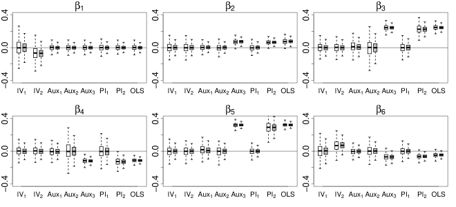
Figure S.6: Bias of estimators in Case 2 of the null treatments setting. White boxes are for sample size 2000 and gray ones for 5000.

S.6.2 Results for the application

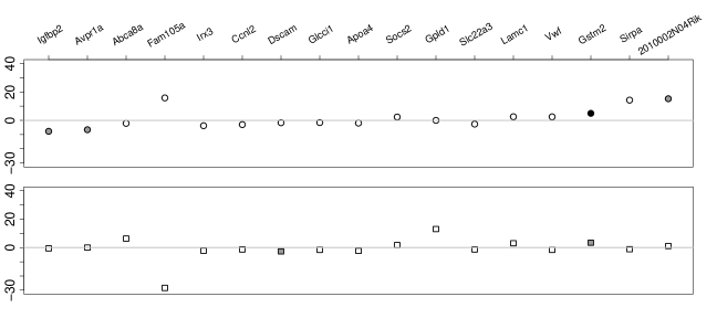
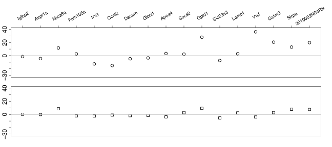
Figure S.7: Effect estimates for 17 genes when two (the first two panels) or three (the last two panels) factors are used in analyses. The first and third panels are for the auxiliary variables estimation, and the second and fourth for the null treatments estimation. Black points are for significant estimates at level of $0.05$, gray ones for $0.1$, and white ones for estimates not significant at $0.1$.

Point and confidence interval estimates

Bootstrap percentiles: 2.5%, 97.5%, 5%, 95%; Significance codes: “**” for significant at level of $0.05$, “*” for $0.1$, and “0” for not significant at level $0.1$.

Estimation with one confounder

1. Results for the auxiliary variables approach

            estimates    2.5%  97.5%      5%    95% significance
Igfbp2        -10.626 -15.614 -5.266 -14.764 -5.719     **
Avpr1a         -8.296 -14.568 -1.544 -13.494 -2.670     **
Abca8a         -5.664 -12.368  1.072 -10.887 -0.032      *
Fam105a        -4.325 -13.812  4.983 -12.137  2.933      0
Irx3           -3.793  -8.033  0.593  -7.297 -0.154      *
Ccnl2          -3.421  -7.810  0.917  -6.966  0.246      0
Dscam          -2.442  -6.703  0.276  -5.072 -0.514      *
Glcci1         -1.429  -6.999  3.139  -5.964  2.360      0
Apoa4          -0.287  -4.226  3.821  -3.569  3.299      0
Socs2           1.162  -1.800  3.909  -1.276  3.516      0
Gpld1           1.456  -6.520 10.827  -4.847  8.951      0
Slc22a3         1.724  -4.953  7.274  -3.915  6.177      0
Lamc1           3.111  -1.267  8.967  -0.661  8.204      0
Vwf             3.410  -2.669  9.452  -1.400  8.589      0
Gstm2           5.717   1.181 10.045   1.864  9.304     **
Sirpa           7.283   1.312 13.743   2.263 12.774     **
2010002N04Rik  10.293   3.012 17.203   4.351 16.110     **


2. Results for the null treatments approach

           estimates    2.5%  97.5%      5%    95% significance
Igfbp2        -1.194  -9.369  2.800  -8.045  1.840      0
Avpr1a        -0.430  -7.574  3.999  -6.821  2.678      0
Abca8a         6.032  -3.043 13.693  -1.842 12.352      0
Fam105a       -6.726 -15.875  3.118 -14.526  1.234      0
Irx3          -2.465  -7.292  1.475  -6.661  0.988      0
Ccnl2         -1.349  -6.031  2.855  -5.338  2.083      0
Dscam         -2.255  -7.043 -0.145  -5.540 -0.390     **
Glcci1        -1.536  -6.826  3.343  -6.151  2.567      0
Apoa4         -2.595  -6.378  2.136  -5.713  1.285      0
Socs2          2.117  -1.100  4.992  -0.533  4.513      0
Gpld1          8.681  -0.709 16.796   0.703 14.594      *
Slc22a3       -1.803  -7.358  4.809  -6.227  3.932      0
Lamc1          2.664  -1.792  8.506  -1.235  7.696      0
Vwf           -1.072  -5.372  6.179  -4.309  5.445      0
Gstm2          3.688  -0.806  9.612   0.171  8.948      *
Sirpa          4.972  -0.704 11.731   0.285 10.628      *
2010002N04Rik  6.272   0.096 13.682   1.353 12.599     **


3. Results for the crude estimation

           estimates    2.5%  97.5%      5%    95% significance
Igfbp2        -8.445 -12.797 -4.586 -12.124 -5.292     **
Avpr1a        -6.607 -11.779 -1.634 -11.094 -2.395     **
Abca8a        -3.236  -8.644  2.049  -7.674  1.429      0
Fam105a       -5.017 -14.030  3.880 -12.662  2.108      0
Irx3          -3.494  -8.028  0.878  -7.284  0.263      0
Ccnl2         -2.962  -7.357  0.860  -6.716  0.269      0
Dscam         -2.410  -7.427 -0.220  -5.806 -0.640     **
Glcci1        -1.522  -7.485  3.178  -6.389  2.303      0
Apoa4         -0.973  -4.563  2.935  -3.992  2.045      0
Socs2          1.518  -1.109  4.289  -0.743  3.828      0
Gpld1          3.919  -2.720 10.907  -1.583  9.980      0
Slc22a3        0.609  -5.184  6.260  -4.205  4.983      0
Lamc1          3.174  -1.191  9.643  -0.598  8.337      0
Vwf            2.032  -3.505  7.896  -2.520  6.781      0
Gstm2          4.767   0.251  9.300   1.194  8.647     **
Sirpa          6.935   0.858 13.027   1.636 12.190     **
2010002N04Rik  9.226   2.454 15.538   3.235 14.574     **

Estimation with two confounders

1. Results for the auxiliary variables approach

           estimates    2.5%  97.5%      5%    95% significance
Igfbp2        -7.707 -18.416  1.113 -16.599 -0.978      *
Avpr1a        -6.586 -15.364  0.383 -13.920 -1.049      *
Abca8a        -2.100 -15.114  8.107 -12.496  5.177      0
Fam105a       15.842 -43.428 59.749 -34.904 49.521      0
Irx3          -3.752  -8.337  0.682  -7.363  0.020      0
Ccnl2         -2.959  -7.808  1.329  -7.060  0.594      0
Dscam         -1.671  -6.691  1.455  -5.357  0.861      0
Glcci1        -1.570  -7.136  3.210  -5.886  2.482      0
Apoa4         -1.913  -7.064  4.566  -5.579  3.704      0
Socs2          2.382  -2.566  6.707  -1.939  5.493      0
Gpld1          0.004  -9.004 11.469  -6.927  9.564      0
Slc22a3       -2.617 -15.306 11.915 -11.466  9.435      0
Lamc1          2.585  -1.511  9.001  -1.086  8.108      0
Vwf            2.503  -3.897  9.630  -2.735  8.523      0
Gstm2          4.962   0.284 10.218   1.271  9.119     **
Sirpa         14.276  -6.498 30.434  -2.951 26.550      0
2010002N04Rik 15.232  -2.550 31.459   0.999 25.530      *


2. Results for the null treatments approach

            estimates    2.5%  97.5%      5%    95% significance
Igfbp2         -0.584   -9.401  2.190  -7.986  1.276      0
Avpr1a          0.021   -8.330  2.998  -7.046  2.156      0
Abca8a          6.359   -3.449 13.216  -2.241 11.147      0
Fam105a       -28.398 -318.341  1.951 -73.696  0.404      0
Irx3           -2.211   -7.370  1.553  -6.523  1.022      0
Ccnl2          -1.270   -6.192  2.666  -5.442  2.121      0
Dscam          -2.692   -7.175  0.208  -5.986 -0.262      *
Glcci1         -1.582   -6.935  3.447  -5.972  2.602      0
Apoa4          -2.275   -6.315  2.239  -5.450  1.679      0
Socs2           1.784   -1.301  5.008  -0.813  4.409      0
Gpld1          13.077   -0.993 19.818  -0.040 17.053      0
Slc22a3        -1.340   -9.239  5.508  -7.669  4.482      0
Lamc1           3.058   -1.893  8.703  -1.245  7.451      0
Vwf            -1.619   -5.267  6.335  -4.201  5.598      0
Gstm2           3.426   -0.295  9.968   0.438  9.129      *
Sirpa          -1.141   -6.001 14.311  -3.833 12.380      0
2010002N04Rik   1.116   -2.534 14.654  -1.160 13.157      0

Estimation with three confounders

1. Results for the auxiliary variables approach

            estimates    2.5%  97.5%      5%    95% significance
Igfbp2         -1.312 -17.987  6.862 -15.951  4.212      0
Avpr1a         -4.481 -18.904  5.022 -15.353  2.897      0
Abca8a         11.713 -17.207 34.518 -12.953 28.557      0
Fam105a         2.648 -71.350 81.166 -49.248 62.241      0
Irx3          -12.628 -33.805  4.268 -24.106  1.251      0
Ccnl2         -15.119 -23.126  4.215 -18.271  1.616      0
Dscam          -4.751 -15.444  1.729 -11.027  0.785      0
Glcci1         -3.485  -9.837  4.176  -7.731  3.013      0
Apoa4           3.268  -7.404 10.427  -5.519  7.904      0
Socs2           2.249  -5.602  8.652  -3.800  6.912      0
Gpld1          28.073 -50.673 59.428 -19.273 42.508      0
Slc22a3        -7.413 -23.712 12.482 -18.348  9.988      0
Lamc1           2.841  -2.863 13.409  -1.291 10.471      0
Vwf            36.274 -11.822 56.152  -4.906 43.160      0
Gstm2          20.551  -4.118 30.792  -0.593 25.547      0
Sirpa          13.029  -6.271 33.161  -3.244 26.817      0
2010002N04Rik  19.805  -6.478 69.222  -0.918 53.812      0


2. Results for the null treatments approach

            estimates    2.5%  97.5%      5%    95% significance
Igfbp2         0.304    -9.903   1.264   -8.630  0.689      0
Avpr1a        -0.188    -8.836   3.601   -7.821  2.650      0
Abca8a         8.709    -4.579  13.954   -3.275 10.415      0
Fam105a       -2.115 -1527.892  42.311 -900.908  6.914      0
Irx3          -2.364    -7.044   4.262   -6.313  2.759      0
Ccnl2         -0.936    -5.863   4.479   -5.029  3.555      0
Dscam         -1.812    -6.532   1.339   -5.410  0.149      0
Glcci1        -1.523    -6.817   3.630   -5.850  2.827      0
Apoa4         -3.665    -7.561   2.568   -6.635  1.677      0
Socs2          2.812    -1.284   5.211   -0.670  4.579      0
Gpld1          9.310    -4.096  19.869   -2.003 15.753      0
Slc22a3       -5.310    -7.903   5.516   -6.701  4.519      0
Lamc1          2.353    -2.483   9.319   -1.486  7.890      0
Vwf           -3.877   -15.989   5.917  -11.843  4.612      0
Gstm2          2.807    -3.831   9.466   -2.007  8.653      0
Sirpa          7.923    -4.153  13.763   -2.283 12.411      0
2010002N04Rik  7.609   -19.287 178.871   -2.461 14.933      0

References

- Alter et al. (2000) Alter, O., Brown, P. O., and Botstein, D. “Singular value decomposition for genome-wide expression data processing and modeling.” Proceedings of the National Academy of Sciences, 97:10101–10106 (2000).
- Anderson and Rubin (1956) Anderson, T. W. and Rubin, H. “Statistical inference in factor analysis.” In Proceedings of the Third Berkeley Symposium on Mathematical Statistics and Probability, Volume 5: Contributions to Econometrics, Industrial Research, and Psychometry, 111–150. Berkeley, Calif.: University of California Press (1956).
- Andrews (2017) Andrews, D. W. “Examples of -complete and boundedly-complete distributions.” Journal of Econometrics, 199:213–220 (2017).
- Angrist et al. (1996) Angrist, J., Imbens, G., and Rubin, D. “Identification of causal effects using instrumental variables.” Journal of the American Statistical Association, 91:444–455 (1996).
- Athey et al. (2019) Athey, S., Imbens, G. W., and Pollmann, M. “Comment on: “The blessings of multiple causes” by Yixin Wang and David M. Blei.” Journal of the American Statistical Association, 114:1602–1604 (2019).
- Bai and Ng (2002) Bai, J. and Ng, S. “Determining the number of factors in approximate factor models.” Econometrica, 70(1):191–221 (2002).
- Balke and Pearl (1997) Balke, A. and Pearl, J. “Bounds on treatment effects from studies with imperfect compliance.” Journal of the American Statistical Association, 92:1171–1176 (1997).
- Basu (1955) Basu, D. “On statistics independent of a complete sufficient statistic.” Sankhya, 15:377–380 (1955).
- Canay et al. (2013) Canay, I. A., Santos, A., and Shaikh, A. M. “On the testability of identification in some nonparametric models with endogeneity.” Econometrica, 81:2535–2559 (2013).
- Carrasco et al. (2007) Carrasco, M., Florens, J. P., and Renault, E. “Linear inverse problems in structural econometrics estimation based on spectral decomposition and regularization.” In Heckman, J. J. and Leamer, E. (eds.), Handbook of Econometrics, volume 6B, 5633–5751. Amsterdam: Elsevier (2007).
- Carroll et al. (2006) Carroll, R., Ruppert, D., Stefanski, L., and Crainiceanu, C. Measurement Error in Nonlinear Models: A Modern Perspective. Boca Raton: Chapman & Hall/CRC, 2nd edition (2006).
- Ćevid et al. (2020) Ćevid, D., Bühlmann, P., and Meinshausen, N. “Spectral deconfounding via perturbed sparse linear models.” Journal of Machine Learning Research, 21:232 (2020).
- Chae et al. (2019) Chae, M., Martin, R., and Walker, S. G. “On an algorithm for solving Fredholm integrals of the first kind.” Statistics and Computing, 29:645–654 (2019).
- Chen et al. (2012) Chen, J., Li, P., and Fu, Y. “Inference on the order of a normal mixture.” Journal of the American Statistical Association, 107:1096–1105 (2012).
- Chen et al. (2014) Chen, X., Chernozhukov, V., Lee, S., and Newey, W. K. “Local identification of nonparametric and semiparametric models.” Econometrica, 82:785–809 (2014).
- Chernozhukov and Hansen (2005) Chernozhukov, V. and Hansen, C. “An IV model of quantile treatment effects.” Econometrica, 73:245–261 (2005).
- Chernozhukov et al. (2017) Chernozhukov, V., Hansen, C., Liao, Y., et al. “A lava attack on the recovery of sums of dense and sparse signals.” The Annals of Statistics, 45:39–76 (2017).
- Cornfield et al. (1959) Cornfield, J., Haenszel, W., Hammond, E. C., Lilienfeld, A. M., Shimkin, M. B., and Wynder, E. L. “Smoking and lung cancer: Recent evidence and a discussion of some questions.” Journal of the National Cancer Institute, 22:173–203 (1959).
- Cox and Donnelly (2011) Cox, D. R. and Donnelly, C. A. Principles of Applied Statistics. Cambridge University Press (2011).
- D’Amour (2019a) D’Amour, A. “On multi-cause causal inference with unobserved confounding: Counterexamples, impossibility, and alternatives.” In The 22nd International Conference on Artificial Intelligence and Statistics, 3478–3486. Okinawa, Japan (2019a).
- D’Amour (2019b) D’Amour, A. “Comment: Reflections on the deconfounder.” Journal of the American Statistical Association, 114:1597–1601 (2019b).
- Darolles et al. (2011) Darolles, S., Fan, Y., Florens, J. P., and Renault, E. “Nonparametric instrumental regression.” Econometrica, 79:1541–1565 (2011).
- D’Haultfœuille (2010) D’Haultfœuille, X. “A new instrumental method for dealing with endogenous selection.” Journal of Econometrics, 154:1–15 (2010).
- D’Haultfœuille (2011) —. “On the completeness condition in nonparametric instrumental problems.” Econometric Theory, 27:460–471 (2011).
- Didelez and Sheehan (2007) Didelez, V. and Sheehan, N. “Mendelian randomization as an instrumental variable approach to causal inference.” Statistical Methods in Medical Research, 16:309–330 (2007).
- Ding and Vanderweele (2014) Ding, P. and Vanderweele, T. J. “Generalized Cornfield conditions for the risk difference.” Biometrika, 101:971–977 (2014).
- Flanders et al. (2017) Flanders, W. D., Strickland, M. J., and Klein, M. “A new method for partial correction of residual confounding in time-series and other observational studies.” American Journal of Epidemiology, 185:941–949 (2017).
- Friguet et al. (2009) Friguet, C., Kloareg, M., and Causeur, D. “A factor model approach to multiple testing under dependence.” Journal of the American Statistical Association, 104:1406–1415 (2009).
- Gagnon-Bartsch and Speed (2012) Gagnon-Bartsch, J. A. and Speed, T. P. “Using control genes to correct for unwanted variation in microarray data.” Biostatistics, 13:539–552 (2012).
- Goldberger (1972) Goldberger, A. S. “Structural equation methods in the social sciences.” Econometrica, 40:979–1001 (1972).
- Gray et al. (2008) Gray, D. L., O’Brien, K. D., D’Alessio, D. A., Brehm, B. J., and Deeg, M. A. “Plasma glycosylphosphatidylinositol-specific phospholipase D predicts the change in insulin sensitivity in response to a low-fat but not a low-carbohydrate diet in obese women.” Metabolism, 57:473–478 (2008).
- Grimmer et al. (2020) Grimmer, J., Knox, D., and Stewart, B. M. “Naive regression requires weaker assumptions than factor models to adjust for multiple cause confounding.” arXiv preprint arXiv:2007.12702 (2020).
- Guo et al. (2020) Guo, Z., Ćevid, D., and Bühlmann, P. “Doubly debiased lasso: High-Dimensional inference under hidden confounding and measurement errors.” arXiv preprint arXiv:2004.03758 (2020).
- Hu and Schennach (2008) Hu, Y. and Schennach, S. M. “Instrumental variable treatment of nonclassical measurement error models.” Econometrica, 76:195–216 (2008).
- Hu and Shiu (2018) Hu, Y. and Shiu, J.-L. “Nonparametric identification using instrumental variables: Sufficient conditions for completeness.” Econometric Theory, 34:659–693 (2018).
- Imai and Jiang (2019) Imai, K. and Jiang, Z. “Comment: The challenges of multiple causes.” Journal of the American Statistical Association, 114:1605–1610 (2019).
- Imbens and Newey (2009) Imbens, G. W. and Newey, W. K. “Identification and estimation of triangular simultaneous equations models without additivity.” Econometrica, 77:1481–1512 (2009).
- Kang et al. (2016) Kang, H., Zhang, A., Cai, T. T., and Small, D. S. “Instrumental variables estimation with some invalid instruments and its application to Mendelian randomization.” Journal of the American Statistical Association, 111:132–144 (2016).
- Kim and Mueller (1978) Kim, J.-O. and Mueller, C. W. Factor Analysis: Statistical Methods and Practical Issues. Beverly Hills, CA: Sage (1978).
- Kong et al. (2021) Kong, D., Yang, S., and Wang, L. “Multi-cause causal inference with unmeasured confounding and binary outcome.” Biometrika, in press (2021).
- Kotlarski (1967) Kotlarski, I. “On characterizing the gamma and the normal distribution.” Pacific Journal of Mathematics, 20:69–76 (1967).
- Kress (1989) Kress, R. Linear Integral Equations. Berlin: Springer (1989).
- Kuroki and Pearl (2014) Kuroki, M. and Pearl, J. “Measurement bias and effect restoration in causal inference.” Biometrika, 101:423–437 (2014).
- Leek and Storey (2007) Leek, J. T. and Storey, J. D. “Capturing heterogeneity in gene expression studies by surrogate variable analysis.” PLoS Genet, 3:e161 (2007).
- Lehman and Scheffe (1950) Lehman, E. and Scheffe, H. “Completeness, Similar Regions and Unbiased Tests. Part I.” Sankhya, 10:219–236 (1950).
- Lin et al. (2015) Lin, W., Feng, R., and Li, H. “Regularization methods for high-dimensional instrumental variables regression with an application to genetical genomics.” Journal of the American Statistical Association, 110:270–288 (2015).
- Lipsitch et al. (2010) Lipsitch, M., Tchetgen Tchetgen, E., and Cohen, T. “Negative controls: A tool for detecting confounding and bias in observational studies.” Epidemiology, 21:383–388 (2010).
- Luo and Wei (2019) Luo, X. and Wei, Y. “Batch effects correction with unknown subtypes.” Journal of the American Statistical Association, 114:581–594 (2019).
- Manski (1990) Manski, C. F. “Nonparametric bounds on treatment effects.” The American Economic Review, 80:319–323 (1990).
- Mattner (1992) Mattner, L. “Completeness of location families, translated moments, and uniqueness of charges.” Probability Theory and Related Fields, 92:137–149 (1992).
- McLachlan et al. (2019) McLachlan, G. J., Lee, S. X., and Rathnayake, S. I. “Finite mixture models.” Annual Review of Statistics and Its Application, 6:355–378 (2019).
- Miao et al. (2018) Miao, W., Geng, Z., and Tchetgen Tchetgen, E. “Identifying causal effects with proxy variables of an unmeasured confounder.” Biometrika, 105:987–993. (2018).
- Miao and Tchetgen Tchetgen (2018) Miao, W. and Tchetgen Tchetgen, E. “A Confounding Bridge Approach for Double Negative Control Inference on Causal Effects.” (2018).
- Miao and Tchetgen Tchetgen (2016) Miao, W. and Tchetgen Tchetgen, E. J. “On varieties of doubly robust estimators under missingness not at random with a shadow variable.” Biometrika, 103(2):475–482 (2016).
- Newey and Powell (2003) Newey, W. K. and Powell, J. L. “Instrumental variable estimation of nonparametric models.” Econometrica, 71:1565–1578 (2003).
- Ogburn et al. (2015) Ogburn, E. L., Rotnitzky, A., and Robins, J. M. “Doubly robust estimation of the local average treatment effect curve.” Journal of the Royal Statistical Society. Series B, Statistical methodology, 77:373–396 (2015).
- Ogburn et al. (2019) Ogburn, E. L., Shpitser, I., and Tchetgen Tchetgen, E. J. “Comment on “Blessings of Multiple Causes”.” Journal of the American Statistical Association, 114:1611–1615 (2019).
- Ogburn et al. (2020) —. “Counterexamples to “The Blessings of Multiple Causes” by Wang and Blei.” arXiv preprint arXiv:2001.06555 (2020).
- Ogburn and VanderWeele (2012) Ogburn, E. L. and VanderWeele, T. J. “On the nondifferential misclassification of a binary confounder.” Epidemiology, 23:433–439 (2012).
- Ogburn and VanderWeele (2013) —. “Bias attenuation results for nondifferentially mismeasured ordinal and coarsened confounders.” Biometrika, 100:241–248 (2013).
- Owen et al. (2016) Owen, A. B., Wang, J., et al. “Bi-cross-validation for factor analysis.” Statistical Science, 31:119–139 (2016).
- Pearl (1995) Pearl, J. “Causal diagrams for empirical research.” Biometrika, 82:669–688 (1995).
- Price et al. (2006) Price, A. L., Patterson, N. J., Plenge, R. M., Weinblatt, M. E., Shadick, N. A., and Reich, D. “Principal components analysis corrects for stratification in genome-wide association studies.” Nature Genetics, 38:904–909 (2006).
- Richardson and Robins (2014) Richardson, T. S. and Robins, J. M. “ACE bounds; SEMs with equilibrium conditions.” Statistical Science, 29:363–366 (2014).
- Robins (1986) Robins, J. “A new approach to causal inference in mortality studies with a sustained exposure period—application to control of the healthy worker survivor effect.” Mathematical Modelling, 7:1393–1512 (1986).
- Robins (1994) Robins, J. M. “Correcting for non-compliance in randomized trials using structural nested mean models.” Communications in Statistics-Theory and Methods, 23:2379–2412 (1994).
- Rosenbaum and Rubin (1983) Rosenbaum, P. R. and Rubin, D. B. “Assessing sensitivity to an unobserved binary covariate in an observational study with binary outcome.” Journal of the Royal Statistical Society: Series B, 45:212–218 (1983).
- Rousseeuw and Leroy (2005) Rousseeuw, P. J. and Leroy, A. M. Robust Regression and Outlier Detection, volume 589. John wiley & sons (2005).
- Schneeberger (2019) Schneeberger, M. “Irx3, a new leader on obesity genetics.” EBioMedicine, 39:19–20 (2019).
- Shi et al. (2020) Shi, X., Miao, W., Nelson, J. C., and Tchetgen Tchetgen, E. “Multiply robust causal inference with double negative control adjustment for categorical unmeasured confounding.” Journal of the Royal Statistical Society: Series B, 82:521–540 (2020).
- Small et al. (2017) Small, D. S., Tan, Z., Ramsahai, R. R., Lorch, S. A., Brookhart, M. A., et al. “Instrumental variable estimation with a stochastic monotonicity assumption.” Statistical Science, 32:561–579 (2017).
- Tchetgen Tchetgen et al. (2020) Tchetgen Tchetgen, E. J., Ying, A., Cui, Y., Shi, X., and Miao, W. “An introduction to proximal causal learning.” arXiv preprint arXiv:2009.10982 (2020).
- Titterington et al. (1985) Titterington, D. M., Smith, A. F., and Makov, U. E. Statistical Analysis of Finite Mixture Distributions. New York: Wiley (1985).
- Wang et al. (2017) Wang, J., Zhao, Q., Hastie, T., and Owen, A. B. “Confounder adjustment in multiple hypothesis testing.” The Annals of Statistics, 45:1863–1894 (2017).
- Wang and Tchetgen Tchetgen (2018) Wang, L. and Tchetgen Tchetgen, E. “Bounded, efficient and multiply robust estimation of average treatment effects using instrumental variables.” Journal of the Royal Statistical Society: Series B, 80:531–550 (2018).
- Wang et al. (2006) Wang, S., Yehya, N., Schadt, E. E., Wang, H., Drake, T. A., and Lusis, A. J. “Genetic and genomic analysis of a fat mass trait with complex inheritance reveals marked sex specificity.” PLoS Genetics, 2:e15 (2006).
- Wang and Blei (2019) Wang, Y. and Blei, D. M. “The blessings of multiple causes.” Journal of the American Statistical Association, 114:1574–1596 (2019).
- Wang and Blei (2020) Wang, Y. and Blei, D. M. “Towards clarifying the theory of the deconfounder.” arXiv preprint arXiv:2003.04948 (2020).
- Wheatcroft et al. (2007) Wheatcroft, S. B., Kearney, M. T., Shah, A. M., Ezzat, V. A., Miell, J. R., Modo, M., Williams, S. C., Cawthorn, W. P., Medina-Gomez, G., Vidal-Puig, A., Sethi, J. K., and Crossey, P. A. “IGF-binding protein-2 protects against the development of obesity and insulin resistance.” Diabetes, 56:285–294 (2007).
- Wright (1928) Wright, P. G. Tariff on Animal and Vegetable Oils. New York: Macmillan (1928).