High dimensional PCA: a new model selection criterion

Abhinav Chakraborty
Department of Statistics
The Wharton School
University of Pennsylvania
Philadelphia, PA 19104, USA
abch@wharton.upenn.edu
   Soumendu Sundar Mukherjee
Interdisciplinary Statistical Research Unit
Applied Statistics Division
Indian Statistical Institute
Kolkata, WB-700108, India
soumendu041@gmail.com
   Arijit Chakrabarti
Applied Statistics Unit
Applied Statistics Division
Indian Statistical Institute
Kolkata, WB-700108, India
arc@isical.ac.in
Abstract

Suppose we have a random sample from a multivariate population consisting of many variables. Estimating the number of dominant/large eigenvalues of the population covariance matrix based on the sample information is an important question arising in Statistics with wide applications in many areas. In the context of Principal Components Analysis (PCA), the linear combinations of the original variables having the largest amounts of variation are determined by this number. In this paper, we study the high dimensional asymptotic setting where the number of variables grows at the same rate as the number of observations. We work in the framework where the population covariance matrix is assumed to have the spiked structure proposed in Johnstone, (2001)). In this setup, the problem of interest becomes essentially one of model selection and has attracted a lot of interest from researchers. Our focus is on the Akaike Information Criterion (AIC) which is known to be strongly consistent from the work of Bai et al., (2018). The result of Bai et al., (2018) requires a certain “gap condition” ensuring that the dominant eigenvalues of the covariance matrix are all above a level which is strictly larger than a threshold discovered by Baik, Ben Arous and Peche (called the BBP threshold), both quantities depending on the limiting ratio of the number of variables and observations. It is well-known in the literature that, below this threshold, a spiked covariance structure becomes indistinguishable from one with no spikes. Thus the strong consistency of AIC requires in a sense some extra “signal strength” than what the BBP threshold corresponds to.

In this paper, our aim is to investigate whether consistency continues to hold even if the “gap” is made smaller. In this regard, we make two novel theoretical contributions. Firstly, we show that strong consistency under arbitrarily small gap is achievable if we alter the penalty term of AIC suitably depending on the target gap. Inspired by this result, we are able to show that a further intuitive alteration of the penalty can indeed make the gap exactly zero, although we can only achieve weak consistency in this case. We compare the two newly-proposed estimators with other existing estimators in the literature via extensive simulation studies, and show, by suitably calibrating our proposals, that a significant improvement in terms of mean-squared error is achievable.

AMS 2010 Mathematics Subject Classifications: 62H12, 62H25 Keywords: Spiked model; model selection; high dimensional PCA

1 Introduction

Suppose we have a sample of observations from a multivariate population with p𝑝p variables. Estimating the number of dominant/significant eigenvalues of the population covariance matrix in such a scenario is an important question arising in Statistics with wide applications in many areas. In the context of Principal Components Analysis (PCA), a very popular method of dimension reduction for multivariate data, the individual principal components having the largest variability are determined by this number.

Let λ1λ2λpsubscript𝜆1subscript𝜆2subscript𝜆𝑝\lambda_{1}\geq\lambda_{2}\geq\cdots\geq\lambda_{p} be the eigenvalues of the population covariance matrix. We further assume that the covariance matrix has a spiked structure proposed by Johnstone, (2001). In this framework, the number of dominant eigenvalues is denoted by k𝑘k and all the eigenvalues except the first k𝑘k are all assumed equal, i.e. λ1λ2λk>λk+1=λk+2==λpsubscript𝜆1subscript𝜆2subscript𝜆𝑘subscript𝜆𝑘1subscript𝜆𝑘2subscript𝜆𝑝\lambda_{1}\geq\lambda_{2}\geq\cdots\geq\lambda_{k}>\lambda_{k+1}=\lambda_{k+2}=\cdots=\lambda_{p}. This k𝑘k is called the true number of dominant/significant components in this framework.

The spiked covariance model finds wide applications in many scientific fields. In wireless communications, for example, a signal emitted by a source is modulated and received by several antennas, and the quality of reconstruction of the original signal is directly linked to the “inference” of spikes. The spiked model is also used in different areas of Artificial Intelligence such as face, handwriting and speech recognition and statistical learning. See Johnstone and Paul, (2018) for more applications.

The number of significant components k𝑘k is usually unknown, and we need to estimate it, which in turn becomes essentially a problem of model selection in the spiked covariance framework. This will be explained clearly in the next section. Many estimators have been developed in the literature, mostly based on information theoretic criteria, such as the minimum description length (MDL), Bayesian Information Criterion (BIC) and Akaike Information Criterion (AIC) (see, e.g., Wax and Kailath, (1985)). However, these applications have been focused on the large sample size and low dimensional regimes and arguments in support of these estimators may not carry over to the high dimensional setup. In the recent past, several works have appeared in the area of signal processing for high dimensional data, where techniques from random matrix theory (RMT) it have been used (see, for example, Kritchman and Nadler, (2009) and Nadler, (2010)). More recent papers in the literature include Passemier and Yao, (2014) and Bai et al., (2018).

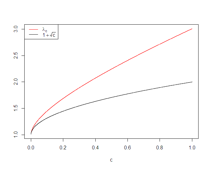
Our work is inspired by Bai et al., (2018), where the authors consider the Akaike Information Criterion (AIC) (Akaike, (1998)) and the Bayesian Information Criterion (BIC) (Schwarz et al., (1978)) as their estimation criterion in a high dimensional setting. They studied the consistency of the estimators based on the AIC and BIC criteria under an asymptotic framework where p,n𝑝𝑛p,n\to\infty such that p/nc>0𝑝𝑛𝑐0p/n\to c>0, where n𝑛n refers to the sample size. They showed that unlike AIC, the BIC criterion is not consistent when the signal strength λksubscript𝜆𝑘\lambda_{k} is bounded (Bai et al., (2018)); in other words BIC requires much more signal strength for signal detection. Their main result shows consistency of AIC for estimating k𝑘k, when a certain “gap condition” is satisfied, i.e. when λksubscript𝜆𝑘\lambda_{k} is above a certain level λcsubscript𝜆𝑐\lambda_{c} above the BBP threshold (Baik et al., (2005)) of 1+c1𝑐1+\sqrt{c} (see Section 2.2). More precisely, they showed that AIC is consistent if and only if λk>λc>1+csubscript𝜆𝑘subscript𝜆𝑐1𝑐\lambda_{k}>\lambda_{c}>1+\sqrt{c}. Figure 1 shows the “gap” between λcsubscript𝜆𝑐\lambda_{c} and 1+c1𝑐1+\sqrt{c}. We want to highlight the fact that if λk1+csubscript𝜆𝑘1𝑐\lambda_{k}\leq 1+\sqrt{c}, then there is no hope for estimating k𝑘k, (see, for example, Baik et al., (2005) and Section 2.1.1 for more details).
Refer to caption
Figure 1: Gap between λcsubscript𝜆𝑐\lambda_{c} and the BBP threshold.

The primary aim our work is to investigate if we can improve upon the results of Bai et al., (2018) by suitably modifying the AIC criterion to give consistent estimates of k𝑘k under weakening of the “gap condition”. Towards this, our main contributions are as follows. We have shown that, given any δ>0𝛿0\delta>0, we can develop an estimator (depending on δ𝛿\delta) which is strongly consistent when the gap between λksubscript𝜆𝑘\lambda_{k} and the BBP threshold is at least δ𝛿\delta (see Section 3.1). We can also make the gap exactly zero by modifying our estimator, but then we have to part with strong consistency-we can only prove weak consistency of the modified estimator (see Section 3.2). We note that there is another weakly-consistent estimator due to Passemier and Yao, (2014) that is known in the literature and which also works under zero gap.

The inspection of the proof of strong consistency in Bai et al., (2018) reveals that for any arbitrary δ>0𝛿0\delta>0, a modification (based on δ𝛿\delta and ratio of dimension and sample size) of the penalty of AIC will make the asymptotic argument work when the gap between λksubscript𝜆𝑘\lambda_{k} and the BBP threshold is above δ𝛿\delta. A further modification of the penalty term by letting that δ𝛿\delta go to zero at appropriate rate depending on n𝑛n gives us an estimator that is weakly consistency under ‘zero gap’. This proof is obtained by employing novel arguments aided by some deep Random Matrix Theory results on the asymptotic behavior of sample covariance matrices.

After finishing this work, it came to our notice that a similar problem has been studied independently by Hu et al., (2020). However, their motivations, results and methods of proof are different from ours.

The rest of the paper is organised as follows. In Section 2, we discuss the problem setup, review some key results of Random Matrix Theory (RMT) and the literature on estimating the number of spikes. Section 3 introduces the main idea and results behind our modified AIC criterion. In Section 4 we compare our proposed estimator with other estimators available in the literature via extensive simulation studies. Conclusions then follow and the Appendix collects all the proofs.

2 Problem setup and a review of relevant literature

We first describe our setup and main problem in the first few paragraphs of this section. We follow the same notations as used in Bai et al., (2018). Suppose we have a random sample 𝐲𝟏,,𝐲𝐧subscript𝐲1subscript𝐲𝐧\mathbf{y_{1},\ldots,y_{n}} of size n𝑛n from a population of dimension p𝑝p and let 𝐘=(𝐲𝟏,,𝐲𝐧)T𝐘superscriptsubscript𝐲1subscript𝐲𝐧𝑇\mathbf{Y}=(\mathbf{y_{1},\ldots,y_{n}})^{T} denote the full (n×p)𝑛𝑝(n\times p) data matrix. Let the population mean be μ𝜇\mathbf{\mu} and population covariance matrix is denoted by 𝚺𝚺\mathbf{\Sigma}. Our interest here is in the spiked covariance structure described before which can be succinctly described through models Mksubscript𝑀𝑘M_{k}, where

Mk:λ1λ2λk>λk+1==λp.:subscript𝑀𝑘subscript𝜆1subscript𝜆2subscript𝜆𝑘subscript𝜆𝑘1subscript𝜆𝑝M_{k}:\lambda_{1}\geq\lambda_{2}\geq\cdots\geq\lambda_{k}>\lambda_{k+1}=\cdots=\lambda_{p}.

We consider models M0,M1,,Mp1subscript𝑀0subscript𝑀1subscript𝑀𝑝1M_{0},M_{1},\ldots,M_{p-1} starting from a configuration of zero spikes (i.e. λ1==λpsubscript𝜆1subscript𝜆𝑝\lambda_{1}=\cdots=\lambda_{p}) to one with (p1)𝑝1(p-1) spikes. We want to estimate, using the available data, the true value of k𝑘k. So our main problem is thus reduced to one of model selection from the pool of the above p𝑝p candidate models.

Our focus in this paper will be the high dimensional asymptotic setting where p𝑝p and n𝑛n grow proportionately, i.e. we assume that

p/nc>0.𝑝𝑛𝑐0p/n\to c>0. (C1)

To avoid notational clutter, we suppress the dependence of p𝑝p on n𝑛n, and of 𝚺𝚺\mathbf{\Sigma},λ1,λ2subscript𝜆1subscript𝜆2\lambda_{1},\lambda_{2}\ldots on p𝑝p. For the estimation of k𝑘k, we will be interested in the study (to be explained later in this section) of the distributional properties of the eigenvalues of the sample covariance matrix of the 𝐲𝐣subscript𝐲𝐣\mathbf{y_{j}}’. We can assume without any loss of generality that μ=0𝜇0\mathbf{\mu}=0. Then the sample covariance matrix 𝐒𝐧subscript𝐒𝐧\mathbf{S_{n}} is given by

𝐒𝐧=1n1i=1n𝐲𝐢𝐲𝐢T.subscript𝐒𝐧1𝑛1superscriptsubscript𝑖1𝑛subscript𝐲𝐢superscriptsubscript𝐲𝐢𝑇\mathbf{S_{n}}=\frac{1}{n-1}\sum_{i=1}^{n}\mathbf{y_{i}}\mathbf{y_{i}}^{T}.

Denoting {1,,n}1𝑛\{1,\ldots,n\} by [n]delimited-[]𝑛[n], we may also assume, as in Bai et al., (2018), that 𝐲𝐣=𝚺12𝐱𝐣subscript𝐲𝐣superscript𝚺12subscript𝐱𝐣\mathbf{y_{j}}=\mathbf{\Sigma}^{\frac{1}{2}}\mathbf{x_{j}} for j[n]𝑗delimited-[]𝑛j\in[n], where 𝐱𝐤=(x1k,,xpk)Tsubscript𝐱𝐤superscriptsubscript𝑥1𝑘subscript𝑥𝑝𝑘𝑇\mathbf{x_{k}}=(x_{1k},\ldots,x_{pk})^{T}, and {xij,i[n],j[n]}formulae-sequencesubscript𝑥𝑖𝑗𝑖delimited-[]𝑛𝑗delimited-[]𝑛\{x_{ij},i\in[n],j\in[n]\} is a double array of i.i.d. random variables with mean 00, variance 111. We further assume, as in Bai et al., (2018), that the xijsubscript𝑥𝑖𝑗x_{ij}’s have finite with finite fourth moment.

For the rest of the paper we assume that the eigenvalues of population covariance matrix 𝚺𝚺\mathbf{\Sigma} are 1 except the first k𝑘k which are (λi)1iksubscriptsubscript𝜆𝑖1𝑖𝑘(\lambda_{i})_{1\leq i\leq k} and 𝚺𝚺\mathbf{\Sigma} has the form

𝚺=(𝚺𝐤𝟎𝟎𝐈𝐩𝐤)𝚺matrixsubscript𝚺𝐤00subscript𝐈𝐩𝐤\mathbf{\Sigma}=\begin{pmatrix}\mathbf{\Sigma_{k}}&\mathbf{0}\\ \mathbf{0}&\mathbf{I_{p-k}}\end{pmatrix} (C2)

where 𝚺𝐤subscript𝚺𝐤\mathbf{\Sigma_{k}} has k𝑘k non-null and non-unit eigenvalues λ1λ2λk>1subscript𝜆1subscript𝜆2subscript𝜆𝑘1\lambda_{1}\geq\lambda_{2}\geq\cdots\geq\lambda_{k}>1. We also assume, as in Bai et al., (2018) that k𝑘k is unknown but a fixed finite number and does not change with n𝑛n.

We will now summarize in the next few subsections, the concepts, issues and results from the literature which are relevant in this study. We will first touch upon some fundamental results on the properties of the eigenstructure of the sample covariance matrix and the high dimensional phenomenon. This will be followed by review of some specific works in the literature on the topic of our interest.

2.1 Basic results on the eigen-structure of sample covariance matrix

We start this section by briefly describing Principal Components Analysis (PCA) since the eigenstructure of the sample covariance matrix is intrinsically related to this. We recall that in PCA (see, e.g., Anderson, (1958); Jolliffe, (1986)), one sequentially finds orthogonal directions to produce uncorrelated (normalized) linear combinations of the original variables with maximum variance. In the standard approach to this, this is obtained from the eigen-decomposition of the (sample)covariance matrix. Consider the eigen-decomposition of ΣΣ\Sigma:

𝚺=λ1𝐮𝟏𝐮𝟏++λp𝐮𝐩𝐮𝐩=𝐔𝚲𝐔,𝚺subscript𝜆1subscript𝐮1superscriptsubscript𝐮1subscript𝜆𝑝subscript𝐮𝐩superscriptsubscript𝐮𝐩𝐔𝚲superscript𝐔\mathbf{\Sigma}=\lambda_{1}\mathbf{u_{1}u_{1}^{\prime}}+\cdots+\lambda_{p}\mathbf{u_{p}u_{p}^{\prime}}=\mathbf{U\Lambda U^{\prime}},

where 𝐔𝐔\mathbf{U} is a p×p𝑝𝑝p\times p orthogonal matrix whose columns are the eigenvector 𝐮𝐢subscript𝐮𝐢\mathbf{u_{i}} and 𝚲𝚲\mathbf{\Lambda} is a diagonal matrix with entries λisubscript𝜆𝑖\lambda_{i} being the eigenvalues of 𝚺𝚺\mathbf{\Sigma}. The sample analogue of this is

𝐒𝐧=l1𝐯𝟏𝐯𝟏++lp𝐯𝐩𝐯𝐩=𝐕𝐋𝐕,subscript𝐒𝐧subscript𝑙1subscript𝐯1superscriptsubscript𝐯1subscript𝑙𝑝subscript𝐯𝐩superscriptsubscript𝐯𝐩superscript𝐕𝐋𝐕\mathbf{S_{n}}=l_{1}\mathbf{v_{1}v_{1}^{\prime}}+\cdots+l_{p}\mathbf{v_{p}v_{p}^{\prime}}=\mathbf{VLV}^{\prime},

where now the orthogonal matrix 𝐕𝐕\mathbf{V} has columns which are the sample eigenvectors 𝐯𝐢subscript𝐯𝐢\mathbf{v_{i}} and 𝐋𝐋\mathbf{L} is a diagonal matrix consisting of the eigenvalues lisubscript𝑙𝑖l_{i} of 𝐒𝐧subscript𝐒𝐧\mathbf{S_{n}}. If 𝐙𝐙\mathbf{Z} denotes a generic random observation from the distribution, then the vector of the population principal components is given by 𝐙𝐔𝐙𝐔\mathbf{ZU}. The sample principal components are defined as 𝐘𝐯𝐢subscript𝐘𝐯𝐢\mathbf{Yv_{i}}, for i=1,,p𝑖1𝑝i=1,\cdots,p. It may be noted that for each i{1,,p}𝑖1𝑝i\in\{1,\cdots,p\}, the variance of 𝐙𝐮𝐢subscript𝐙𝐮𝐢\mathbf{Zu_{i}} is λisubscript𝜆𝑖\lambda_{i}. So larger the λisubscript𝜆𝑖\lambda_{i}, larger is the variance of random variable 𝐙𝐮𝐢subscript𝐙𝐮𝐢\mathbf{Zu_{i}}. Thus the number of dominant/large eigenvalues of 𝚺𝚺\mathbf{\Sigma} correspond to the number of principal components having the largest amount of information. In the traditional fixed dimensional setting where p𝑝p is fixed, and n𝑛n is large, the sample eigenvalues and eigenvectors converge to their population counterparts, i.e. as n𝑛n\to\infty, we have that lia.s.λil_{i}\overset{a.s.}{\to}\lambda_{i} and via.s.uiv_{i}\overset{a.s.}{\to}u_{i}, for each i=1,,p𝑖1𝑝i=1,\cdots,p (see, for example, Anderson, (1958)). The situation is more subtle in the high dimensional case where p𝑝p grows with n𝑛n and it is well-known in the literature (Silverstein, (1995)) that the consistency of the sample eigenvalues and eigenvectors do not carry over in this case. In the next part of this section we focus on the high-dimensional aspect with special emphasis on results from random matrix theory under the spiked covariance framework.

2.1.1 The high dimensional phenomenon and Random Matrix Theory results

Many of the things described below are classically well-known facts from Random Matrix Theory (RMT) and some are more recent interesting discoveries. The notational convention is similar to Bai et al., (2018). Recall that the eigenvalues of 𝐒𝐧subscript𝐒𝐧\mathbf{S_{n}} are denoted by l1l2lp0subscript𝑙1subscript𝑙2subscript𝑙𝑝0l_{1}\geq l_{2}\geq\cdots\geq l_{p}\geq 0 ( again suppressing their dependence on n𝑛n and/or p𝑝p). Let us define the Empirical Spectral Distribution (ESD) of 𝐒𝐧subscript𝐒𝐧\mathbf{S_{n}} by

Fn(x)=1pi=1p𝟙{lix}.subscript𝐹𝑛𝑥1𝑝superscriptsubscript𝑖1𝑝1subscript𝑙𝑖𝑥F_{n}(x)=\frac{1}{p}\sum_{i=1}^{p}\mathbbm{1}\{l_{i}\leq x\}.

By a result of Silverstein, (1995) we have that under condition (C2) the ESD of 𝐒𝐧subscript𝐒𝐧\mathbf{S_{n}}, i.e. Fn(x)subscript𝐹𝑛𝑥F_{n}(x) converges to Fc(x)subscript𝐹𝑐𝑥F_{c}(x) almost surely, where Fc(x)subscript𝐹𝑐𝑥F_{c}(x) is the Marčhenco-Pastur law/distribution. Here, for 0<c10𝑐10<c\leq 1, Fcsubscript𝐹𝑐F_{c} is given by

Fc(x)=fc(x)=12πxc(bx)(xa).superscriptsubscript𝐹𝑐𝑥subscript𝑓𝑐𝑥12𝜋𝑥𝑐𝑏𝑥𝑥𝑎F_{c}^{\prime}(x)=f_{c}(x)=\frac{1}{2\pi xc}\sqrt{(b-x)(x-a)}.

The support of this distribution is [a,b]𝑎𝑏[a,b] where a:=(1c)2assign𝑎superscript1𝑐2a:=(1-\sqrt{c})^{2} and b:=(1+c)2assign𝑏superscript1𝑐2b:=(1+\sqrt{c})^{2}.

If c>1𝑐1c>1, Fcsubscript𝐹𝑐F_{c} has a point mass 11/c11𝑐1-1/c at the origin, i.e.

Fc(x)={0if x<0,11/cif 0x<a,11/c+axfc(t)𝑑tif axb,subscript𝐹𝑐𝑥cases0if 𝑥011𝑐if 0𝑥𝑎11𝑐superscriptsubscript𝑎𝑥subscript𝑓𝑐𝑡differential-d𝑡if 𝑎𝑥𝑏F_{c}(x)=\begin{cases}0&\text{if }x<0,\\ 1-1/c&\text{if }0\leq x<a,\\ 1-1/c+\int_{a}^{x}f_{c}(t)dt&\text{if }a\leq x\leq b,\end{cases}

where a𝑎a and b𝑏b are the same as in the case 0<c10𝑐10<c\leq 1.

The previous result characterizes the bulk behaviour of the sample eigenvalues. Now we state results characterizing convergence of individual eigenvalues of 𝐒𝐧subscript𝐒𝐧\mathbf{S_{n}}. As in Bai et al., (2018), we define λisubscript𝜆𝑖\lambda_{i} to be a “distant spiked eigenvalue” if λi>1+csubscript𝜆𝑖1𝑐\lambda_{i}>1+\sqrt{c}. We also define the function ψc(x)subscript𝜓𝑐𝑥\psi_{c}(x) for x1𝑥1x\neq 1 as

ψc(x)=x+cxx1.subscript𝜓𝑐𝑥𝑥𝑐𝑥𝑥1\psi_{c}(x)=x+\frac{cx}{x-1}.

This next result is the same as Lemma 2.1 in Bai et al., (2018).

Lemma 2.1.

Let lisubscript𝑙𝑖l_{i} denote the i-th largest eigenvalue of 𝐒𝐧subscript𝐒𝐧\mathbf{S_{n}} the covariance matrix in our setup. Suppose that 𝔼(x114)<𝔼superscriptsubscript𝑥114\mathbb{E}(x_{11}^{4})<\infty, conditions (C1)C1(\ref{eq:C1}) and (C2)C2(\ref{eq:C2}) hold, and that λ1subscript𝜆1\lambda_{1} is bounded.

  • (i)

    If λisubscript𝜆𝑖\lambda_{i} is distant-spiked, then lia.s.ψc(λi)=ψi=λi+cλiλi1l_{i}\overset{a.s.}{\to}\psi_{c}(\lambda_{i})=\psi_{i}=\lambda_{i}+\frac{c\lambda_{i}}{\lambda_{i}-1}.

  • (ii)

    If λisubscript𝜆𝑖\lambda_{i} is not distant-spiked and i/pα𝑖𝑝𝛼i/p\to\alpha, then lia.s.μ1αl_{i}\overset{a.s.}{\to}\mu_{1-\alpha}, where μαsubscript𝜇𝛼\mu_{\alpha} is the α𝛼\alpha-quantile of the MP distribution. In particular, if i=o(p)𝑖𝑜𝑝i=o(p), then lia.s.μ1=b=(1+c)2l_{i}\overset{a.s.}{\to}\mu_{1}=b=(1+\sqrt{c})^{2}.

The results in the above lemma are examples of a general high dimensional “phase transition” phenomenon observed by many authors (e.g., Bai and Yao, (2012), Baik et al., (2005)), and often referred as the BBP phase transition phenomenon after Baik et al., (2005). In a nutshell, as summarized in Paul, (2007), this refers to the fact that if the non-unit eigenvalues of a spiked model are close to one, then their sample counterparts would asymptotically behave as if the true covariance matrix were the identity matrix. However, the asymptotics would change critically if the dominant eigenvalues are larger than the threshold of (1+c)1𝑐(1+\sqrt{c}). We describe its details and the implications on our assumptions.
For understanding its effect on distributional convergence, we assume now for simplicity that 𝚺𝚺\mathbf{\Sigma} is diagonal with a single spike (k=1𝑘1k=1), so that 𝚺=diag{λ1,1,,1}𝚺diagsubscript𝜆111\mathbf{\Sigma}=\mathrm{diag}\{\lambda_{1},1,\cdots,1\}. When λ1=1subscript𝜆11\lambda_{1}=1, the largest sample eigenvalue is located near the upper edge b𝑏b of the MP distribution and fluctuates on the (small) scale n2/3superscript𝑛23n^{-2/3} approximately according to the real valued Tracy-Widom distribution:

n23l1μ(c)σ(c)𝑑TW1,superscript𝑛23subscript𝑙1𝜇𝑐𝜎𝑐𝑑𝑇subscript𝑊1n^{\frac{2}{3}}\frac{l_{1}-\mu(c)}{\sigma(c)}\overset{d}{\to}TW_{1},

where μ(c)=b𝜇𝑐𝑏\mu(c)=b and σ(c)=(1+c)4/3c1/6𝜎𝑐superscript1𝑐43superscript𝑐16\sigma(c)=(1+\sqrt{c})^{4/3}c^{-1/6} and TW1𝑇subscript𝑊1TW_{1} is a random variable following real valued TW distribution (see Johnstone, (2001) for more details). For λ11+csubscript𝜆11𝑐\lambda_{1}\leq 1+\sqrt{c}, the largest sample eigenvalue has the same limiting Tracy-Widom distribution-the small spike in the top population eigenvalue has no limiting effect on the distribution of sample top eigenvalue. Put in another way, asymptotically the largest sample eigenvalue is of no use in detecting a subcritical spike in the largest population eigenvalue. A phase transition occurs at 1+c1𝑐1+\sqrt{c} : for larger values of λ1subscript𝜆1\lambda_{1}, the largest sample eigenvalue l1subscript𝑙1l_{1} now has a limiting Gaussian distribution (See Paul, (2007)), with scale on the usual order of n1/2superscript𝑛12n^{-1/2}. The mean of this Gaussian distribution (=ψ(λ1)𝜓subscript𝜆1\psi(\lambda_{1})) shows a significant upward bias, being significantly larger than the true value of λ1subscript𝜆1\lambda_{1}. We now come back briefly to the manifestation of the phase transition in the issue of pointwise convergence as in Lemma 2.1, where we consider a spiked model of k𝑘k spikes. For the non spiked eigenvalue λk+1subscript𝜆𝑘1\lambda_{k+1}, the sample counterpart lk+1subscript𝑙𝑘1l_{k+1} converges a.s. to (1+c)2superscript1𝑐2(1+\sqrt{c})^{2} (by the Lemma 2.1 (ii)). If 1<λk1+c1subscript𝜆𝑘1𝑐1<\lambda_{k}\leq 1+\sqrt{c} then lksubscript𝑙𝑘l_{k} also converges a.s. to (1+c)2superscript1𝑐2(1+\sqrt{c})^{2}. So asymptotically it becomes difficult to distinguish lksubscript𝑙𝑘l_{k} and lk+1subscript𝑙𝑘1l_{k+1} (i.e. model Mksubscript𝑀𝑘M_{k} and Mk+1subscript𝑀𝑘1M_{k+1} respectively). This is not the case if λk>1+csubscript𝜆𝑘1𝑐\lambda_{k}>1+\sqrt{c} as seen in Lemma 2.1 (i)). Keeping in mind this phase transition behaviour, we have assumed for our results presented later that the first k𝑘k eigenvalues are “distant spiked eigenvalues”

2.2 Strongly consistent estimators based on AIC

This section is mainly based on the paper by Bai et al., (2018). They consider the spiked covariance structure mentioned before which is expressed by models denoted by Mksubscript𝑀𝑘M_{k}’s for varying k𝑘k depending on the value of the true number of spikes k𝑘k. To estimate k𝑘k, they propose using the traditional AIC criterion to select a model from among the pool of candidate models and thereby obtain an estimator which is strongly consistent. We shall discuss the pn𝑝𝑛p\leq n case first. Defining

Cp,n=nlog((n1)/n)p+np{1+log(2π)},C_{p,n}=n\log((n-1)/n)^{p}+np\{1+\log(2\pi)\},

it has been noted in in Fujikoshi et al., (2011) that the criterion value under model Mjsubscript𝑀𝑗M_{j} is given by

AICj=nlog(l1lj)+n(pj)logl¯j+2dj+Cp,n,subscriptAIC𝑗𝑛subscript𝑙1subscript𝑙𝑗𝑛𝑝𝑗subscript¯𝑙𝑗2subscript𝑑𝑗subscript𝐶𝑝𝑛\mathrm{AIC}_{j}=n\log(l_{1}\ldots l_{j})+n(p-j)\log\bar{l}_{j}+2d_{j}+C_{p,n},

where l1>>lpsubscript𝑙1subscript𝑙𝑝l_{1}>\ldots>l_{p} are the sample eigenvalues of 𝐒𝐧subscript𝐒𝐧\mathbf{S_{n}} and for 1jp11𝑗𝑝11\leq j\leq p-1, l¯jsubscript¯𝑙𝑗\bar{l}_{j} is the arithmetic mean of lj+1,,lpsubscript𝑙𝑗1subscript𝑙𝑝l_{j+1},\ldots,l_{p}, that is,

l¯j=1pjt=j+1plt.subscript¯𝑙𝑗1𝑝𝑗superscriptsubscript𝑡𝑗1𝑝subscript𝑙𝑡\bar{l}_{j}=\frac{1}{p-j}\sum_{t=j+1}^{p}l_{t}.

Furthermore, djsubscript𝑑𝑗d_{j} denotes the number of independent model parameters under model Mjsubscript𝑀𝑗M_{j} and is given by

djsubscript𝑑𝑗\displaystyle d_{j} =pj12j(j+1)+j+1+pabsent𝑝𝑗12𝑗𝑗1𝑗1𝑝\displaystyle=pj-\frac{1}{2}j(j+1)+j+1+p
=(j+1)(p+1j/2).absent𝑗1𝑝1𝑗2\displaystyle=(j+1)(p+1-j/2).

The expression of djsubscript𝑑𝑗d_{j} is obtained by looking at the eigen-decomposition of the covariance matrix ΣΣ\Sigma which can be written as:

Σ=i=1jλiuiuiT+λ(Ii=1juiuiT),Σsuperscriptsubscript𝑖1𝑗subscript𝜆𝑖subscript𝑢𝑖superscriptsubscript𝑢𝑖𝑇𝜆𝐼superscriptsubscript𝑖1𝑗subscript𝑢𝑖superscriptsubscript𝑢𝑖𝑇\Sigma=\sum_{i=1}^{j}\lambda_{i}u_{i}u_{i}^{T}+\lambda(I-\sum_{i=1}^{j}u_{i}u_{i}^{T}),

where uisubscript𝑢𝑖u_{i}’s are mutually orthogonal unit vectors. It is evident that p𝑝p degrees of freedom are accounted for by μ𝜇\mu, j+1𝑗1j+1 by λisubscript𝜆𝑖\lambda_{i}’s i=1,j𝑖1𝑗i=1,\ldots j and λ𝜆\lambda, and pjj(j+1)/2𝑝𝑗𝑗𝑗12pj-j(j+1)/2 by the j𝑗j orthonormal eigen-vectors. The AIC criterion selects the model Mk^Asubscript𝑀subscript^𝑘𝐴M_{\hat{k}_{A}} where

k^A=arg minjAICj.subscript^𝑘𝐴subscriptarg min𝑗subscriptAIC𝑗\hat{k}_{A}=\text{arg min}_{j}\mathrm{AIC}_{j}.

The estimator of k𝑘k proposed by Bai et al., (2018) is k^Asubscript^𝑘𝐴\hat{k}_{A}. When we are interested in only the first q𝑞q models Mj,j=0,1,,q1formulae-sequencesubscript𝑀𝑗𝑗01𝑞1M_{j},j=0,1,\ldots,q-1, then the criteria is defined by considering the minimum only with respect to j=0,1,,q1𝑗01𝑞1j=0,1,\ldots,q-1. We call q𝑞q the number of candidate models. Denoting Aj=1n(AICjAICp1)subscript𝐴𝑗1𝑛subscriptAIC𝑗subscriptAIC𝑝1A_{j}=\frac{1}{n}(\mathrm{AIC}_{j}-\mathrm{AIC}_{p-1}), the model selection rule of AIC can be equivalently obtained as

k^A=arg minjAj.subscript^𝑘𝐴subscriptarg min𝑗subscript𝐴𝑗\hat{k}_{A}=\text{arg min}_{j}A_{j}.

Note that Ajsubscript𝐴𝑗A_{j} is given by

Aj=(pj)logl¯ji=j+1plogli(pj1)(pj+2)n.subscript𝐴𝑗𝑝𝑗subscript¯𝑙𝑗superscriptsubscript𝑖𝑗1𝑝subscript𝑙𝑖𝑝𝑗1𝑝𝑗2𝑛A_{j}=(p-j)\log\bar{l}_{j}-\sum_{i=j+1}^{p}\log l_{i}-\frac{(p-j-1)(p-j+2)}{n}.

We are now going to state main results of Bai et al., (2018) regarding consistency of k^Asubscript^𝑘𝐴\hat{k}_{A}. A criterion k^^𝑘\hat{k} for estimating k𝑘k is said to be consistent (strongly consistent) if limnP(k^=k)=1subscript𝑛𝑃^𝑘𝑘1\lim_{n\to\infty}P(\hat{k}=k)=1 [ P(limnk^=k)=1𝑃subscript𝑛^𝑘𝑘1P(\lim_{n\to\infty}\hat{k}=k)=1.

We will first state the result for the case 0<c10𝑐10<c\leq 1. Before stating the result, we state condition (C3) referred to as the “gap condition”. Recalling the function ψc(x)subscript𝜓𝑐𝑥\psi_{c}(x) and quantities ψi=ψc(λi)subscript𝜓𝑖subscript𝜓𝑐subscript𝜆𝑖\psi_{i}=\psi_{c}(\lambda_{i}) defined earlier, the “gap condition” is given by

ψk1logψk2c>0.subscript𝜓𝑘1subscript𝜓𝑘2𝑐0\psi_{k}-1-\log\psi_{k}-2c>0. (C3)

The next result is proved as Theorem 3.1(i) of Bai et al., (2018).

Theorem 2.2.

Suppose the conditions (C1) with 0<c10𝑐10<c\leq 1, and (C2) hold, and that the number of candidate models, q𝑞q, satisfies q=o(p)𝑞𝑜𝑝q=o(p). Suppose also that λ1subscript𝜆1\lambda_{1} is bounded.We have the following results on the consistency of the estimation criterion k^Asubscript^𝑘𝐴\hat{k}_{A} based on AIC:

  • (i)

    If the gap condition (C3) does not hold, then k^Asubscript^𝑘𝐴\hat{k}_{A} is not consistent.

  • (ii)

    If the gap condition (C3) holds, then k^Asubscript^𝑘𝐴\hat{k}_{A} is strongly consistent.

Next we consider the case where p,n𝑝𝑛p,n\to\infty, such that p>n𝑝𝑛p>n and p/nc>1𝑝𝑛𝑐1p/n\to c>1. Clearly in this setup the smallest p(n1)𝑝𝑛1p-(n-1) eigenvalues of 𝐒𝐧subscript𝐒𝐧\mathbf{S_{n}} are zero, that is,

ln1>ln==lp=0.subscript𝑙𝑛1subscript𝑙𝑛subscript𝑙𝑝0l_{n-1}>l_{n}=\ldots=l_{p}=0.

Thus, as noted in Bai et al., (2018), it is impossible to infer about the smallest population eigenvalues λn,λn+1,,λp>0subscript𝜆𝑛subscript𝜆𝑛1subscript𝜆𝑝0\lambda_{n},\lambda_{n+1},\ldots,\lambda_{p}>0 using the sample eigenvalues. Therefore, these authors additionally assume in this setup that (C4) holds where

λn1=λn==λp=1.subscript𝜆𝑛1subscript𝜆𝑛subscript𝜆𝑝1\lambda_{n-1}=\lambda_{n}=\ldots=\lambda_{p}=1. (C4)

Under this new assumption, for j=0,1,,n2𝑗01𝑛2j=0,1,\ldots,n-2, it follows that

M~j:λj>λj+1==λn1Mj:λj>λj+1==λp.:subscript~𝑀𝑗subscript𝜆𝑗subscript𝜆𝑗1subscript𝜆𝑛1subscript𝑀𝑗:subscript𝜆𝑗subscript𝜆𝑗1subscript𝜆𝑝\tilde{M}_{j}:\lambda_{j}>\lambda_{j+1}=\ldots=\lambda_{n-1}\Leftrightarrow M_{j}:\lambda_{j}>\lambda_{j+1}=\ldots=\lambda_{p}.

In order to describe the model selection criterion proposed in this setup in Bai et al., (2018), l¯jsubscript¯𝑙𝑗\bar{l}_{j} first has to be redefined as below:

l¯j=1n1jt=j+1n1ltj=1,2,,n1.formulae-sequencesubscript¯𝑙𝑗1𝑛1𝑗superscriptsubscript𝑡𝑗1𝑛1subscript𝑙𝑡𝑗12𝑛1\bar{l}_{j}=\frac{1}{n-1-j}\sum_{t=j+1}^{n-1}l_{t}\quad\quad j=1,2,\ldots,n-1.

Using this modification, a new criterion Aj~~subscript𝐴𝑗\tilde{A_{j}} is then introduced as

Aj~=(n1j)logl¯ji=j+1n1logli(nj2)(nj+1)p,~subscript𝐴𝑗𝑛1𝑗subscript¯𝑙𝑗superscriptsubscript𝑖𝑗1𝑛1subscript𝑙𝑖𝑛𝑗2𝑛𝑗1𝑝\tilde{A_{j}}=(n-1-j)\log\bar{l}_{j}-\sum_{i=j+1}^{n-1}\log l_{i}-\frac{(n-j-2)(n-j+1)}{p},

by replacing the p𝑝p and n𝑛n in Ajsubscript𝐴𝑗A_{j} by n1𝑛1n-1 and p𝑝p, respectively. Note that A~n2=0subscript~𝐴𝑛20\tilde{A}_{n-2}=0. The “quasi-AIC” rule, henceforth abbreviated as the qAIC rule, selects the model k^A~subscript^𝑘~𝐴\hat{k}_{\tilde{A}} defined as

k^A~=arg minjn2A~j.subscript^𝑘~𝐴subscriptarg min𝑗𝑛2subscript~𝐴𝑗\hat{k}_{\tilde{A}}=\text{arg min}_{j\leq n-2}\tilde{A}_{j}.

The strong consistency result of qAIC for the case c>1𝑐1c>1 is proved under the modified “gap condition”

ψk/c1log(ψk/c)2/c>0.subscript𝜓𝑘𝑐1subscript𝜓𝑘𝑐2𝑐0\psi_{k}/c-1-\log(\psi_{k}/c)-2/c>0. (C5)

We now state the result regarding consistency of k^A~subscript^𝑘~𝐴\hat{k}_{\tilde{A}} proved as Theorem 3.3(i) in Bai et al., (2018).

Theorem 2.3.

Suppose the conditions (C1) with c>1𝑐1c>1, and (C4) hold, and that the number of candidate models, q𝑞q, satisfies q=o(p)𝑞𝑜𝑝q=o(p). Suppose also that λ1subscript𝜆1\lambda_{1} is bounded. We have the following results on the consistency of the estimation criterion k^A~subscript^𝑘~𝐴\hat{k}_{\tilde{A}} based on qAIC:

  • (i)

    If the gap condition (C5) fails, then k^A~subscript^𝑘~𝐴\hat{k}_{\tilde{A}} is not consistent.

  • (ii)

    If the gap condition (C5) holds, then k^A~subscript^𝑘~𝐴\hat{k}_{\tilde{A}} is strongly consistent.

Next we will discuss another type of estimators available in the literature which are weakly consistent, i.e. if k^^𝑘\hat{k} is an estimator of k𝑘k then k^𝑝k^𝑘𝑝𝑘\hat{k}\overset{p}{\to}k as n𝑛n\to\infty.

2.3 Weak consistency

This section is based on the work of Passemier and Yao, (2014) where they proposed a weakly consistent estimator of k𝑘k under the “zero gap” condition. Suppose we have observed a random sample 𝐲𝐢,,𝐲𝐧subscript𝐲𝐢subscript𝐲𝐧\mathbf{y_{i},\ldots,y_{n}} from a p𝑝p-dimensional population. These authors additionally assumed that the 𝐲𝐲\mathbf{y}’s can be expressed as 𝐲=𝐄𝐕12𝐱𝐲superscript𝐄𝐕12𝐱\mathbf{y}=\mathbf{EV}^{\frac{1}{2}}\mathbf{x}, where 𝐱p𝐱superscript𝑝\mathbf{x}\in\mathbb{R}^{p} is a zero-mean random vector of i.i.d. components, 𝐄𝐄\mathbf{E} is an orthogonal matrix and

𝐕=cov(𝐱)=(𝚺𝐤𝟎𝟎𝐈𝐩𝐤),𝐕cov𝐱matrixsubscript𝚺𝐤00subscript𝐈𝐩𝐤\mathbf{V}=\mathrm{cov}(\mathbf{x})=\begin{pmatrix}\mathbf{\Sigma_{k}}&\mathbf{0}\\ \mathbf{0}&\mathbf{I_{p-k}}\end{pmatrix},

where 𝚺𝐤subscript𝚺𝐤\mathbf{\Sigma_{k}} has k𝑘k non-null and non-unit eigenvalues λ1λ2λk>1subscript𝜆1subscript𝜆2subscript𝜆𝑘1\lambda_{1}\geq\lambda_{2}\geq\cdots\geq\lambda_{k}>1. The sample covariance matrix is taken to be

𝐒𝐧=1ni=1n𝐲𝐢𝐲𝐢.subscript𝐒𝐧1𝑛superscriptsubscript𝑖1𝑛subscript𝐲𝐢superscriptsubscript𝐲𝐢\mathbf{S_{n}}=\frac{1}{n}\sum_{i=1}^{n}\mathbf{y_{i}y_{i}}^{\prime}.

The proposed estimator in Passemier and Yao, (2014) is based on the differences between consecutive eigenvalues of 𝐒𝐧subscript𝐒𝐧\mathbf{S_{n}}. The main idea behind that is explained next. Define δjsubscript𝛿𝑗\delta_{j} as

δj=ljlj+1, for j=1,,p1.formulae-sequencesubscript𝛿𝑗subscript𝑙𝑗subscript𝑙𝑗1 for 𝑗1𝑝1\delta_{j}=l_{j}-l_{j+1},\mbox{ for }j=1,\cdots,p-1.

The authors then observe that under certain assumptions it can be shown that if jk𝑗𝑘j\geq k then δj0subscript𝛿𝑗0\delta_{j}\to 0 at a fast rate, whereas if j<k𝑗𝑘j<k and λjsubscript𝜆𝑗\lambda_{j}’s are different then δjsubscript𝛿𝑗\delta_{j} tends to a positive limit. Even if λjsubscript𝜆𝑗\lambda_{j}’s are same, for j<k𝑗𝑘j<k, the convergence of δjsubscript𝛿𝑗\delta_{j} to zero is slow. Thus a possible estimate of k𝑘k can be the index j𝑗j where δjsubscript𝛿𝑗\delta_{j} becomes small for the first time. The estimator of k𝑘k proposed in Passemier and Yao, (2014) is denoted by k^Psubscript^𝑘𝑃\hat{k}_{P} and is given by

k^P=min{j{1,,s}:δj+1,p<dn},subscript^𝑘𝑃:𝑗1𝑠subscript𝛿𝑗1𝑝subscript𝑑𝑛\hat{k}_{P}=\min\{j\in\{1,\ldots,s\}:\delta_{j+1,p}<d_{n}\},

where s>k𝑠𝑘s>k is a fixed number big enough, and dnsubscript𝑑𝑛d_{n} is an appropriately chosen small number. In practice, the integer s𝑠s should be thought as a preliminary bound on the number of possible spikes. Before stating the main theorem on weak consistency of this estimator, we state one of the main assumptions which is required to prove their theorem. Assumption 1: The entries xisuperscript𝑥𝑖x^{i} of the random vector 𝐱𝐱\mathbf{x} have a symmetric law and a sub-exponential decay, that is there exists positive constants C,C𝐶superscript𝐶C,C^{\prime} such that, for all tC𝑡superscript𝐶t\geq C^{\prime}

(|xi|tC)et.superscript𝑥𝑖superscript𝑡𝐶superscript𝑒𝑡\mathbb{P}(|x^{i}|\geq t^{C})\leq e^{-t}.
Theorem 2.4.

Let (𝐲𝐢)(1in)subscriptsubscript𝐲𝐢1𝑖𝑛(\mathbf{y_{i}})_{(1\leq i\leq n)} be n𝑛n i.i.d. of 𝐲=𝐄𝐕12𝐱𝐲superscript𝐄𝐕12𝐱\mathbf{y}=\mathbf{EV}^{\frac{1}{2}}\mathbf{x}, where 𝐱p𝐱superscript𝑝\mathbf{x}\in\mathbb{R}^{p} is a zero-mean random vector of i.i.d. components which satisfies Assumption 1. Assume that V𝑉V is of the form described before where 𝚺𝐤subscript𝚺𝐤\mathbf{\Sigma_{k}} has k𝑘k non null, non unit eigenvalues satisfying λ1λk>1+csubscript𝜆1subscript𝜆𝑘1𝑐\lambda_{1}\geq\ldots\geq\lambda_{k}>1+\sqrt{c}. Assume further that (C1) holds. Let dnsubscript𝑑𝑛d_{n} be a real sequence such that dn=o(n12)subscript𝑑𝑛𝑜superscript𝑛12d_{n}=o(n^{-\frac{1}{2}}) and n2/3dnsuperscript𝑛23subscript𝑑𝑛n^{2/3}d_{n}\to\infty, then the estimator k^Psubscript^𝑘𝑃\hat{k}_{P} is a weakly consistent estimator, i.e. (k^P=k)1subscript^𝑘𝑃𝑘1\mathbb{P}(\hat{k}_{P}=k)\to 1 as n𝑛n\to\infty.

3 Main ideas and results

In this section we will motivate and describe the main results of this article. We will first discuss our work on strong consistency followed by that on weak consistency.

3.1 Strong consistency for modified AIC criterion

The idea for developing a modification of the AIC criterion comes from a careful study of the proof of strong consistency of the traditional AIC in Bai et al., (2018). The “gap condition” mentioned before is a crucial requirement in their proof. This makes AIC inadequate for consistent estimation of k𝑘k when λksubscript𝜆𝑘\lambda_{k} is close to the BBP threshold (1+c1𝑐1+\sqrt{c}). We show in this paper that by suitably modifying the penalty term in the AIC criterion, this problem can be taken care of, in that the modified criterion is strong consistent even when λksubscript𝜆𝑘\lambda_{k} is arbitrarily close to 1+c1𝑐1+\sqrt{c}. In this section We will informally sketch how to get this modified criterion and also the proof of its strong consistency. Towards that, let us first recall the functions we defined earlier

h(x)𝑥\displaystyle h(x) =x1logx,absent𝑥1𝑥\displaystyle=x-1-\log x,
ψc(x)subscript𝜓𝑐𝑥\displaystyle\psi_{c}(x) =x+cxx1,absent𝑥𝑐𝑥𝑥1\displaystyle=x+\frac{cx}{x-1},
Fc(x)subscript𝐹𝑐𝑥\displaystyle F_{c}(x) =h(ψc(x)).absentsubscript𝜓𝑐𝑥\displaystyle=h(\psi_{c}(x)). (\star)

3.1.1 Case: 0<c10𝑐10<c\leq 1

Assume that λk>1+csubscript𝜆𝑘1𝑐\lambda_{k}>1+\sqrt{c}. Note that hh is strictly increasing on [1,)1[1,\infty), and ψcsubscript𝜓𝑐\psi_{c} is strictly increasing on [1+c,)1𝑐[1+\sqrt{c},\infty), with ψc(1+c)=(1+c)2=:b\psi_{c}(1+\sqrt{c})=(1+\sqrt{c})^{2}=:b. Therefore Fcsubscript𝐹𝑐F_{c} is also strictly increasing on [1+c,)1𝑐[1+\sqrt{c},\infty).

Next we break down the proof of consistency by Bai et al., (2018) in two main steps. This gives us the important clue on how to modify the penalty of AIC.

  • (i)

    For showing k^Aksubscript^𝑘𝐴𝑘\hat{k}_{A}\leq k a.s., Bai et al., (2018) needed the condition that

    1b+logb+2c>0,1𝑏𝑏2𝑐0\displaystyle 1-b+\log b+2c>0,

    i.e. 2c>Fc(1+c)2𝑐subscript𝐹𝑐1𝑐2c>F_{c}(1+\sqrt{c}), which is true for any c(0,1)𝑐01c\in(0,1) (as can be verified directly).

  • (ii)

    To ensure that k^Aksubscript^𝑘𝐴𝑘\hat{k}_{A}\geq k a.s. Bai et al., (2018) needed the GAP condition (C3):

    ψk1logψk2c>0subscript𝜓𝑘1subscript𝜓𝑘2𝑐0absent\displaystyle\psi_{k}-1-\log\psi_{k}-2c>0\Leftrightarrow\,\, Fc(λk)>2csubscript𝐹𝑐subscript𝜆𝑘2𝑐\displaystyle F_{c}(\lambda_{k})>2c
    \displaystyle\Leftrightarrow\,\, λk>Fc1(2c)=ψc1(h1(2c))=:λc.\displaystyle\lambda_{k}>F_{c}^{-1}(2c)=\psi_{c}^{-1}(h^{-1}(2c))=:\lambda_{c}.

Clearly λc>1+csubscript𝜆𝑐1𝑐\lambda_{c}>1+\sqrt{c}. Let

u(c):=λc(1+c).assign𝑢𝑐subscript𝜆𝑐1𝑐u(c):=\lambda_{c}-(1+\sqrt{c}).

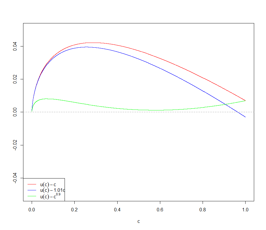
Let u(c)𝑢𝑐u(c) denote the gap between the BBP threshold 1+c1𝑐1+\sqrt{c} and the consistency threshold λcsubscript𝜆𝑐\lambda_{c} for AIC. A natural question is, how large is the gap as a function of c𝑐c? It is displayed in Figure 2. The numerical calculation below shows that u(c)>c𝑢𝑐𝑐u(c)>c ; in fact, u(c)>c0.9𝑢𝑐superscript𝑐0.9u(c)>c^{0.9}.

Refer to caption
Figure 2: The size of the gap u(c)𝑢𝑐u(c).

Our aim here is to investigate if we can develop a criterion that will be strongly consistent even when λksubscript𝜆𝑘\lambda_{k} is closer to 1+c1𝑐1+\sqrt{c} than λcsubscript𝜆𝑐\lambda_{c}. The inequalities in (i) and (ii) above appear in the final asymptotic limits in the argument of Bai et al., (2018). Placed together, for every 0<c10𝑐10<c\leq 1, it is required that the inequalities Fc(λk)>2c>Fc(1+c)subscript𝐹𝑐subscript𝜆𝑘2𝑐subscript𝐹𝑐1𝑐F_{c}(\lambda_{k})>2c>F_{c}(1+\sqrt{c}) hold, where the factor 2 appears unchanged from the per parameter penalty 2 in AIC and c𝑐c from the limiting ratio of p𝑝p and n𝑛n. Our modified AIC criterion is based on the crucial analytic observation we now make. From the monotonicity of of Fc(.)F_{c}(.), the second inequality above also holds if 2 is replaced by any α<2𝛼2\alpha<2 such that Fc(1+c)>αcsubscript𝐹𝑐1𝑐𝛼𝑐F_{c}(1+\sqrt{c})>\alpha c. Evidently, for any fixed c(0,1]𝑐01c\in(0,1], there is whole interval of such choices of α𝛼\alpha, and for that matter, one can choose α𝛼\alpha to make Fc(1+c)subscript𝐹𝑐1𝑐F_{c}(1+\sqrt{c}) arbitrarily close of αc𝛼𝑐\alpha c. For any such α𝛼\alpha, a modified first inequality Fc(λk)<αcsubscript𝐹𝑐subscript𝜆𝑘𝛼𝑐F_{c}(\lambda_{k})<\alpha c will be satisfied by any λksubscript𝜆𝑘\lambda_{k} larger than Fc1(αc))F_{c}^{-1}(\alpha c)), the latter being smaller than λcsubscript𝜆𝑐\lambda_{c} by monotonicity of Fc(.)F_{c}(.). Clearly Fc1(αc)(1+c)<ucsuperscriptsubscript𝐹𝑐1𝛼𝑐1𝑐subscript𝑢𝑐F_{c}^{-1}(\alpha c)-(1+\sqrt{c})<u_{c}. Smaller the choice of α𝛼\alpha, closer is Fc1(αc)superscriptsubscript𝐹𝑐1𝛼𝑐F_{c}^{-1}(\alpha c) to (1+c)1𝑐(1+\sqrt{c}). We derive our modified AIC criterion by formally using this basic observation as described below.

Suppose we modify the original penalty of AIC with α(p/n)𝛼𝑝𝑛\alpha(p/n), for some continuous function α:(0,):𝛼maps-to0\alpha:\mathbb{R}\mapsto(0,\infty), then the same arguments as in Bai et al., (2018) lead to the following conditions:

  • (iii)

    For showing k^αksubscript^𝑘𝛼𝑘\hat{k}_{\alpha}\leq k a.s.,

    1b+logb+α(c)c>0,1𝑏𝑏𝛼𝑐𝑐01-b+\log b+\alpha(c)c>0,

    i.e. α(c)c>Fc(1+c)𝛼𝑐𝑐subscript𝐹𝑐1𝑐\alpha(c)c>F_{c}(1+\sqrt{c}).

  • (iv)

    For showing k^αksubscript^𝑘𝛼𝑘\hat{k}_{\alpha}\geq k a.s.,

    Fc(λk)>α(c)c,subscript𝐹𝑐subscript𝜆𝑘𝛼𝑐𝑐F_{c}(\lambda_{k})>\alpha(c)c,

where k^αsubscript^𝑘𝛼\hat{k}_{\alpha} is the minimizer of this new criterion over the model space. Thus if we want to get a modified criterion that is strongly consistent for any “gap” δc(0,u(c))subscript𝛿𝑐0𝑢𝑐\delta_{c}\in(0,u(c)), all we need is that

α(c)=1cFc(1+c+δc).𝛼𝑐1𝑐subscript𝐹𝑐1𝑐subscript𝛿𝑐\alpha(c)=\frac{1}{c}F_{c}(1+\sqrt{c}+\delta_{c}).

The monotonicity of Fc(.)F_{c}(.) will ensure that the ineualities in (iii) and (iv) will be satisfied for this choice of α(c)𝛼𝑐\alpha(c) which assures strong consistency of k^αsubscript^𝑘𝛼\hat{k}_{\alpha} as long as λk>1+c+δcsubscript𝜆𝑘1𝑐subscript𝛿𝑐\lambda_{k}>1+\sqrt{c}+\delta_{c}. Thus we can reach arbitrarily close to the BBP threshold 1+c1𝑐1+\sqrt{c} and still achieve strong consistency. In fact, since u(c)>c𝑢𝑐𝑐u(c)>c, we may choose δc(0,c]subscript𝛿𝑐0𝑐\delta_{c}\in(0,c]. For example, if we choose δc=c100csubscript𝛿𝑐superscript𝑐100much-less-than𝑐\delta_{c}=c^{100}\ll c, then with

α(c)=1cFc(1+c+c100),𝛼𝑐1𝑐subscript𝐹𝑐1𝑐superscript𝑐100\alpha(c)=\frac{1}{c}F_{c}(1+\sqrt{c}+c^{100}),

we have consistency of k^αsubscript^𝑘𝛼\hat{k}_{\alpha} as long as λk>1+c+c100subscript𝜆𝑘1𝑐superscript𝑐100\lambda_{k}>1+\sqrt{c}+c^{100}. This is a better estimator than AIC because it can consistently estimate k𝑘k even when GAP condition (C3) fails to hold. In particular if we want our gap between λksubscript𝜆𝑘\lambda_{k} and 1+c1𝑐1+\sqrt{c} to be δ𝛿\delta, where δ>0𝛿0\delta>0 is any arbitrarily small constant we can choose α(.)\alpha(.) such that

α(c)=1cFc(1+c+δ),𝛼𝑐1𝑐subscript𝐹𝑐1𝑐𝛿\alpha(c)=\frac{1}{c}F_{c}(1+\sqrt{c}+\delta),

and we would have strong consistency of our estimator as long as λk>1+c+δsubscript𝜆𝑘1𝑐𝛿\lambda_{k}>1+\sqrt{c}+\delta.

We now describe in detail the new model selection criterion which we discussed above. The model selection criterion being a modification of AIC is being called AICsuperscriptAIC\mathrm{AIC}^{*}. Do describe this, we first fix a constant δ>0𝛿0\delta>0. We shall discuss the p<n𝑝𝑛p<n case first. With Cp,nsubscript𝐶𝑝𝑛C_{p,n} as defined before, the criterion value for AICsuperscriptAIC\mathrm{AIC}^{*} for the model Mjsubscript𝑀𝑗M_{j} is defined as

AICj=nlog(l1lj)+n(pj)logl¯j+1p/nFp/n(1+p/n+δ)dj+Cp,n,subscriptsuperscriptAIC𝑗𝑛subscript𝑙1subscript𝑙𝑗𝑛𝑝𝑗subscript¯𝑙𝑗1𝑝𝑛subscript𝐹𝑝𝑛1𝑝𝑛𝛿subscript𝑑𝑗subscript𝐶𝑝𝑛\mathrm{AIC}^{*}_{j}=n\log(l_{1}\ldots l_{j})+n(p-j)\log\bar{l}_{j}+\frac{1}{p/n}F_{p/n}(1+\sqrt{p/n}+\delta)d_{j}+C_{p,n},

where, as before, l1>>lp>0subscript𝑙1subscript𝑙𝑝0l_{1}>\ldots>l_{p}>0 are the sample eigenvalues of 𝐒𝐧subscript𝐒𝐧\mathbf{S_{n}} and for 1jp11𝑗𝑝11\leq j\leq p-1, l¯jsubscript¯𝑙𝑗\bar{l}_{j} is the arithmetic mean of lj+1,,lpsubscript𝑙𝑗1subscript𝑙𝑝l_{j+1},\ldots,l_{p}, that is,

l¯j=1pjt=j+1pltsubscript¯𝑙𝑗1𝑝𝑗superscriptsubscript𝑡𝑗1𝑝subscript𝑙𝑡\bar{l}_{j}=\frac{1}{p-j}\sum_{t=j+1}^{p}l_{t}

and, dj=(j+1)(p+1j/2)subscript𝑑𝑗𝑗1𝑝1𝑗2d_{j}=(j+1)(p+1-j/2) denotes the number of independent parameters in the model under Mjsubscript𝑀𝑗M_{j}. Furthermore the function Fc(.)F_{c}(.) is defined as in (3.1). Then the AICsuperscriptAIC\mathrm{AIC}^{*} selects k𝑘k according to the rule

k^A=arg minjAICj,subscriptsuperscript^𝑘𝐴subscriptarg min𝑗subscriptsuperscriptAIC𝑗\hat{k}^{*}_{A}=\text{arg min}_{j}\mathrm{AIC}^{*}_{j},

where the minimum has been taken over the model space.

Now we state our main result regarding consistency of our estimator k^Asubscriptsuperscript^𝑘𝐴\hat{k}^{*}_{A} whose proof can be found in Appendix Section 7.3.

Theorem 3.1.

Suppose the conditions (C1) with 0<c10𝑐10<c\leq 1, and (C2) hold, and that the number of candidate models, q𝑞q, satisfies q=o(p)𝑞𝑜𝑝q=o(p). Assume that λ1subscript𝜆1\lambda_{1} is bounded. We have the following results on the consistency of the estimation criterion k^Asubscriptsuperscript^𝑘𝐴\hat{k}^{*}_{A} based on AICsuperscriptAIC\mathrm{AIC}^{*}:

  • (i)

    If λk1+c+δsubscript𝜆𝑘1𝑐𝛿\lambda_{k}\leq 1+\sqrt{c}+\delta, then k^Asubscriptsuperscript^𝑘𝐴\hat{k}^{*}_{A} is not consistent.

  • (ii)

    If λk>1+c+δsubscript𝜆𝑘1𝑐𝛿\lambda_{k}>1+\sqrt{c}+\delta, then k^Asubscriptsuperscript^𝑘𝐴\hat{k}^{*}_{A} is strongly consistent.

3.1.2 Case: c>1𝑐1c>1

Next we consider the case where c>1𝑐1c>1. Let

Qc(x)=ch(ψc(x)c).subscript𝑄𝑐𝑥𝑐subscript𝜓𝑐𝑥𝑐Q_{c}(x)=ch\left(\frac{\psi_{c}(x)}{c}\right).

Recall that hh is strictly increasing on [1,)1[1,\infty), and ψcsubscript𝜓𝑐\psi_{c} is strictly increasing on [1+c,)1𝑐[1+\sqrt{c},\infty), Therefore ψc(x)/csubscript𝜓𝑐𝑥𝑐\psi_{c}(x)/c is increasing in x𝑥x. We have ψc(1+c)/c=(1+c)2/c>1c>1formulae-sequencesubscript𝜓𝑐1𝑐𝑐superscript1𝑐2𝑐1for-all𝑐1\psi_{c}(1+\sqrt{c})/c=(1+\sqrt{c})^{2}/c>1\quad\forall c>1. Therefore Qcsubscript𝑄𝑐Q_{c} is also strictly increasing on [1+c,)1𝑐[1+\sqrt{c},\infty).

  • (i)

    For showing k^A~ksubscript^𝑘~𝐴𝑘\hat{k}_{\tilde{A}}\leq k a.s., Bai et al., (2018) needed the condition

    1b/c+log(b/c)+2/c>0,1𝑏𝑐𝑏𝑐2𝑐0\displaystyle 1-b/c+\log(b/c)+2/c>0,

    i.e. 2>Qc(1+c)2subscript𝑄𝑐1𝑐2>Q_{c}(1+\sqrt{c}), which is true for any c>1𝑐1c>1 (as can be verified directly).

  • (ii)

    To ensure that k^A~ksubscript^𝑘~𝐴𝑘\hat{k}_{\tilde{A}}\geq k a.s. Bai et al., (2018) need the GAP condition (C5):

    ψk/c1log(ψk/c)2/c>0Qc(λk)>2λk>Qc1(2)=:λc.\displaystyle\psi_{k}/c-1-\log(\psi_{k}/c)-2/c>0\Leftrightarrow Q_{c}(\lambda_{k})>2\Leftrightarrow\lambda_{k}>Q_{c}^{-1}(2)=:\lambda_{c}.

Note that λc>1+csubscript𝜆𝑐1𝑐\lambda_{c}>1+\sqrt{c}. Let

v(c):=λc(1+c).assign𝑣𝑐subscript𝜆𝑐1𝑐v(c):=\lambda_{c}-(1+\sqrt{c}).

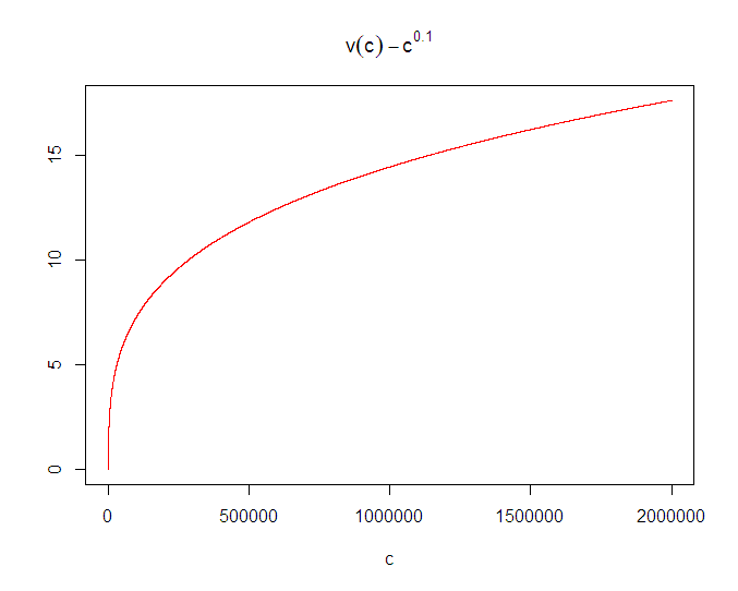
v(c)𝑣𝑐v(c) is the gap between the BBP threshold 1+c1𝑐1+\sqrt{c} and the consistency threshold λcsubscript𝜆𝑐\lambda_{c} for qAIC. Our aim as in the previous case is to investigate if a new criterion can be derived with is strongly consistent even when the “gap” is reduced as much as possible. So firstly we look at how large is the gap as a function of c𝑐c? Figure 3 shows that v(c)>c0.1𝑣𝑐superscript𝑐0.1v(c)>c^{0.1}.

Refer to caption
Figure 3: The size of the gap v(c)𝑣𝑐v(c).

Following similar intuition as in the case of 0<c10𝑐10<c\leq 1, if we penalize by replacing the 222 in qAIC with α(p/n)𝛼𝑝𝑛\alpha(p/n) for some function α:(0,):𝛼maps-to0\alpha:\mathbb{R}\mapsto(0,\infty), then the same arguments as in Bai et al., (2018) lead to the following conditions:

  • (iii)

    For showing k^αksubscript^𝑘𝛼𝑘\hat{k}_{\alpha}\leq k a.s.,

    1b/c+log(b/c)+α(c)/c>0,1𝑏𝑐𝑏𝑐𝛼𝑐𝑐01-b/c+\log(b/c)+\alpha(c)/c>0,

    i.e. α(c)>Qc(1+c)𝛼𝑐subscript𝑄𝑐1𝑐\alpha(c)>Q_{c}(1+\sqrt{c}).

  • (iv)

    For showing k^αksubscript^𝑘𝛼𝑘\hat{k}_{\alpha}\geq k a.s.,

    Qc(λk)>α(c).subscript𝑄𝑐subscript𝜆𝑘𝛼𝑐Q_{c}(\lambda_{k})>\alpha(c).

Thus for any δc(0,v(c))subscript𝛿𝑐0𝑣𝑐\delta_{c}\in(0,v(c)), if we take the function

α(c)=Qc(1+c+δc),𝛼𝑐subscript𝑄𝑐1𝑐subscript𝛿𝑐\alpha(c)=Q_{c}(1+\sqrt{c}+\delta_{c}),

then using the monotonicity of Qc(.)Q_{c}(.) we have consistency of k^αsubscript^𝑘𝛼\hat{k}_{\alpha} as long as λk>1+c+δcsubscript𝜆𝑘1𝑐subscript𝛿𝑐\lambda_{k}>1+\sqrt{c}+\delta_{c}. Thus we can reach arbitrarily close to the BBP threshold 1+c1𝑐1+\sqrt{c}.

Our model selection criterion is a modification of the criterion proposed by Bai et al., (2018) as discussed in Section 2.2. We define our criterion using A~~superscript𝐴\tilde{A^{*}}, which for model Mjsubscript𝑀𝑗M_{j} is given by

Aj~=(n1j)logl¯ji=j+1n1logliQp/n(1+p/n+δ)(nj2)(nj+1)2p~subscriptsuperscript𝐴𝑗𝑛1𝑗subscript¯𝑙𝑗superscriptsubscript𝑖𝑗1𝑛1subscript𝑙𝑖subscript𝑄𝑝𝑛1𝑝𝑛𝛿𝑛𝑗2𝑛𝑗12𝑝\tilde{A^{*}_{j}}=(n-1-j)\log\bar{l}_{j}-\sum_{i=j+1}^{n-1}\log l_{i}-Q_{p/n}(1+\sqrt{p/n}+\delta)\frac{(n-j-2)(n-j+1)}{2p}

where l¯jpsubscript¯𝑙𝑗𝑝\bar{l}_{jp} is defined as in Bai et al., (2018) for p>n𝑝𝑛p>n case which is

l¯j=1ni1t=i+1n1ltsubscript¯𝑙𝑗1𝑛𝑖1superscriptsubscript𝑡𝑖1𝑛1subscript𝑙𝑡\bar{l}_{j}=\frac{1}{n-i-1}\sum_{t=i+1}^{n-1}l_{t}

and Qc(.)Q_{c}(.) is as defined in (3.1.2). The model selection rule A~~superscript𝐴\tilde{A^{*}} estimates k𝑘k by k^A~subscriptsuperscript^𝑘~𝐴\hat{k}^{*}_{\tilde{A}} defined as

k^A~=arg minjA~j,subscriptsuperscript^𝑘~𝐴subscriptarg min𝑗subscript~superscript𝐴𝑗\hat{k}^{*}_{\tilde{A}}=\text{arg min}_{j}\tilde{A^{*}}_{j},

the minimum. as before, being taken over the model space.

The following result shows the consistency of our estimator k^A~subscriptsuperscript^𝑘~𝐴\hat{k}^{*}_{\tilde{A}}.

Theorem 3.2.

Suppose the conditions (C1) with c>1𝑐1c>1 and (C4) hold, and that the number of candidate models, q𝑞q, satisfies q=o(p)𝑞𝑜𝑝q=o(p). Suppose that λ1subscript𝜆1\lambda_{1} is bounded. We have the following results on the consistency of the estimation criterion k^A~subscriptsuperscript^𝑘~𝐴\hat{k}^{*}_{\tilde{A}}:

  • (i)

    If λk1+c+δsubscript𝜆𝑘1𝑐𝛿\lambda_{k}\leq 1+\sqrt{c}+\delta, then k^A~subscript^𝑘~𝐴\hat{k}_{\tilde{A}} is not consistent.

  • (ii)

    If λk>1+c+δsubscript𝜆𝑘1𝑐𝛿\lambda_{k}>1+\sqrt{c}+\delta, then k^A~subscript^𝑘~𝐴\hat{k}_{\tilde{A}} is strongly consistent.

3.2 Weak Consistency for a modified AIC criterion

We have seen in the previous section that for any given δ>0𝛿0\delta>0, however small, we can appropriately modify the penalty term (using δ𝛿\delta among other things) of the usual AIC to produce an estimator of k𝑘k which is strongly consistent when the gap between λksubscript𝜆𝑘\lambda_{k} and the BBP threshold is larger than δ𝛿\delta. But ideally we would aim to develop consistent estimators of k𝑘k which would be consistent if λk>1+csubscript𝜆𝑘1𝑐\lambda_{k}>1+\sqrt{c}, i.e. the we can afford to have the “gap” equal to zero. A natural thing is to first investigate what happens when we choose the gap to be δn>0subscript𝛿𝑛0\delta_{n}>0, where δn0subscript𝛿𝑛0\delta_{n}\to 0 as n𝑛n\rightarrow\infty in the definition of the modified AIC criterion described before.

We first discuss the case 0<c10𝑐10<c\leq 1. We mofify the penalty term in AIC criterion as α(p,n)𝛼𝑝𝑛\alpha(p,n) instead of 222 where

α(p,n)=1p/nFp/n(1+p/n+δn).𝛼𝑝𝑛1𝑝𝑛subscript𝐹𝑝𝑛1𝑝𝑛subscript𝛿𝑛\alpha(p,n)=\frac{1}{p/n}F_{p/n}(1+\sqrt{p/n}+\delta_{n}).

We define k^αsubscript^𝑘𝛼\hat{k}_{\alpha} as the index that minimizes this modified criterion. Observe that

α(p,n)1cFc(1+c) as n.formulae-sequence𝛼𝑝𝑛1𝑐subscript𝐹𝑐1𝑐 as 𝑛\alpha(p,n)\to\frac{1}{c}F_{c}(1+\sqrt{c})\qquad\text{ as }n\to\infty.

Let us check if k^αsubscript^𝑘𝛼\hat{k}_{\alpha} is strongly consistent. Following the arguments of Bai et al., (2018), we find the following.

  • (i)

    For showing k^αksubscript^𝑘𝛼𝑘\hat{k}_{\alpha}\geq k a.s. we need,

    Fc(λk)>Fc(1+c).subscript𝐹𝑐subscript𝜆𝑘subscript𝐹𝑐1𝑐F_{c}(\lambda_{k})>F_{c}(1+\sqrt{c}).

    This is true since we have that λk>1+csubscript𝜆𝑘1𝑐\lambda_{k}>1+\sqrt{c}.

  • (i)

    For showing k^αksubscript^𝑘𝛼𝑘\hat{k}_{\alpha}\leq k a.s. we need,

    1b+logb+Fc(1+c)>0,1𝑏𝑏subscript𝐹𝑐1𝑐01-b+\log b+F_{c}(1+\sqrt{c})>0,

    i.e. Fc(1+c)>Fc(1+c)subscript𝐹𝑐1𝑐subscript𝐹𝑐1𝑐F_{c}(1+\sqrt{c})>F_{c}(1+\sqrt{c}), which is not true.

Clearly the arguments given by Bai et al., (2018) doesn’t give us our desired result for the above intuitive modification of our previous criterion. We however have been able to come up with a novel argument that gives us our desired result. The argument is described in detail in Section 7.2 of the Appendix and carefully exploits some deep results available from Random Matrix Theory regarding the rate of convergence of certain functionals of the sample covariance matrix. Ultimately it turns out that δnsubscript𝛿𝑛\delta_{n} has to converge to zero in such a rate that the new penalty α(p,n)𝛼𝑝𝑛\alpha(p,n) satisfies certain convergence properties. The only downside is that we cannot prove strong consistency of the new criterion using this method, but we can show weak consistency of the estimator under some assumptions (see Theorem 3.3 and 3.4).

As mentioned above, the basic idea for developing the estimator which would be consistent under the “zero” gap condition was to use our previous modified AIC criterion with δnsubscript𝛿𝑛\delta_{n} instead of δ𝛿\delta, where δn0subscript𝛿𝑛0\delta_{n}\to 0. We describe below the model selection rule. This The being a modification of AICsuperscriptAIC\mathrm{AIC}^{*}, we call it AICsuperscriptAICabsent\mathrm{AIC}^{**}. We discuss the p<n𝑝𝑛p<n case first. With Cp,nsubscript𝐶𝑝𝑛C_{p,n} defined as before, the criterion value under model Mjsubscript𝑀𝑗M_{j} is defined as

AICj=nlog(l1lj)+n(pj)logl¯j+1p/nFp/n(1+p/n+δn)dj+Cp,nsubscriptsuperscriptAICabsent𝑗𝑛subscript𝑙1subscript𝑙𝑗𝑛𝑝𝑗subscript¯𝑙𝑗1𝑝𝑛subscript𝐹𝑝𝑛1𝑝𝑛subscript𝛿𝑛subscript𝑑𝑗subscript𝐶𝑝𝑛\mathrm{AIC}^{**}_{j}=n\log(l_{1}\ldots l_{j})+n(p-j)\log\bar{l}_{j}+\frac{1}{p/n}F_{p/n}(1+\sqrt{p/n}+\delta_{n})d_{j}+C_{p,n}

Furthermore, djsubscript𝑑𝑗d_{j} is as defined before. Defining

Aj=1n(AICjAICp1),subscriptsuperscript𝐴absent𝑗1𝑛subscriptsuperscriptAICabsent𝑗subscriptsuperscriptAICabsent𝑝1A^{**}_{j}=\frac{1}{n}(\mathrm{AIC}^{**}_{j}-\mathrm{AIC}^{**}_{p-1}),

we have

Aj=(pj)logl¯ji=j+1plogli1p/nFp/n(1+p/n+δn)(pj1)(pj+2)2nsubscriptsuperscript𝐴absent𝑗𝑝𝑗subscript¯𝑙𝑗superscriptsubscript𝑖𝑗1𝑝subscript𝑙𝑖1𝑝𝑛subscript𝐹𝑝𝑛1𝑝𝑛subscript𝛿𝑛𝑝𝑗1𝑝𝑗22𝑛A^{**}_{j}=(p-j)\log\bar{l}_{j}-\sum_{i=j+1}^{p}\log l_{i}-\frac{1}{p/n}F_{p/n}(1+\sqrt{p/n}+\delta_{n})\frac{(p-j-1)(p-j+2)}{2n}

Then the AICsuperscriptAICabsent\mathrm{AIC}^{**} criterion selects model with index k^Asubscriptsuperscript^𝑘absent𝐴\hat{k}^{**}_{A} obtained as

k^A=arg minjAICj,subscriptsuperscript^𝑘absent𝐴subscriptarg min𝑗subscriptsuperscriptAICabsent𝑗\hat{k}^{**}_{A}=\text{arg min}_{j}\mathrm{AIC}^{**}_{j},

or equivalently

k^A=arg minjAj.subscriptsuperscript^𝑘absent𝐴subscriptarg min𝑗subscriptsuperscript𝐴absent𝑗\hat{k}^{**}_{A}=\text{arg min}_{j}A^{**}_{j}.

The criteria above is defined by considering the minimum only with respect to j=0,1,,s1𝑗01𝑠1j=0,1,\ldots,s-1. where s>k𝑠𝑘s>k is a fixed number big enough. In practice, the integer s𝑠s should be thought as a preliminary bound on the number of possible spikes. We have the following theorem regarding consistency of the proposed estimator whose proof can be found in Appendix Section 7.2.

Theorem 3.3.

Suppose the condition (C1) holds for 0<c10𝑐10<c\leq 1 and (C2) hold, and that that the number of candidate models is s𝑠s, where s>k𝑠𝑘s>k is a fixed number. Suppose that Assumption 1 holds true, λ1subscript𝜆1\lambda_{1} is bounded and λk>1+csubscript𝜆𝑘1𝑐\lambda_{k}>1+\sqrt{c}. Let δnsubscript𝛿𝑛\delta_{n} be a real sequence going to 0 such that

n2/3(Fp/n(1+p/n+δn)Fc(1+c)),superscript𝑛23subscript𝐹𝑝𝑛1𝑝𝑛subscript𝛿𝑛subscript𝐹𝑐1𝑐n^{2/3}\left(F_{p/n}(1+\sqrt{p/n}+\delta_{n})-F_{c}(1+\sqrt{c})\right)\to\infty,

where Fcsubscript𝐹𝑐F_{c} is as defined in (3.1), then the estimator k^Asubscriptsuperscript^𝑘absent𝐴\hat{k}^{**}_{A} is a weakly consistent estimator of k𝑘k, i.e. (k^A=k)1subscriptsuperscript^𝑘absent𝐴𝑘1\mathbb{P}(\hat{k}^{**}_{A}=k)\to 1 as n𝑛n\to\infty.

We have the similar result for the case p>n𝑝𝑛p>n, i.e. c>1𝑐1c>1. Our modified model selection criterion is defined using Aj~superscript~subscript𝐴𝑗absent\tilde{A_{j}}^{**}, which is defined as

Aj~=(n1j)logl¯ji=j+1n1logliQp/n(1+p/n+δn)(nj2)(nj+1)2psuperscript~subscript𝐴𝑗absent𝑛1𝑗subscript¯𝑙𝑗superscriptsubscript𝑖𝑗1𝑛1subscript𝑙𝑖subscript𝑄𝑝𝑛1𝑝𝑛subscript𝛿𝑛𝑛𝑗2𝑛𝑗12𝑝\tilde{A_{j}}^{**}=(n-1-j)\log\bar{l}_{j}-\sum_{i=j+1}^{n-1}\log l_{i}-Q_{p/n}(1+\sqrt{p/n}+\delta_{n})\frac{(n-j-2)(n-j+1)}{2p}

Then Aj~superscript~subscript𝐴𝑗absent\tilde{A_{j}}^{**} selects the number of significant components according to

k^A~=arg minjAj~.subscriptsuperscript^𝑘absent~𝐴subscriptarg min𝑗superscript~subscript𝐴𝑗absent\hat{k}^{**}_{\tilde{A}}=\text{arg min}_{j}\tilde{A_{j}}^{**}.

The criteria above is defined by considering the minimum only with respect to j=0,1,,s1𝑗01𝑠1j=0,1,\ldots,s-1. where s>k𝑠𝑘s>k is a fixed number big enough. In practice, the integer s𝑠s should be thought as a preliminary bound on the number of possible spikes. We have the following theorem regarding consistency of the proposed estimator whose proof can be found in Appendix Section 7.2.

Theorem 3.4.

Suppose the condition (C1) with c>1𝑐1c>1 and (C2) hold, and that that the number of candidate models is s𝑠s, where s>k𝑠𝑘s>k is a fixed number. Suppose that Assumption 1 holds true, λ1subscript𝜆1\lambda_{1} is bounded and λk>1+csubscript𝜆𝑘1𝑐\lambda_{k}>1+\sqrt{c}. We also assume that p/n=c+O(n2/3)𝑝𝑛𝑐𝑂superscript𝑛23p/n=c+O(n^{-2/3}).
Let δnsubscript𝛿𝑛\delta_{n} be a real sequence going to 0 such that

n2/3(1p/nQp/n(1+p/n+δn)1cQc(1+c)),superscript𝑛231𝑝𝑛subscript𝑄𝑝𝑛1𝑝𝑛subscript𝛿𝑛1𝑐subscript𝑄𝑐1𝑐n^{2/3}\left(\frac{1}{p/n}Q_{p/n}(1+\sqrt{p/n}+\delta_{n})-\frac{1}{c}Q_{c}(1+\sqrt{c})\right)\to\infty,

where Qcsubscript𝑄𝑐Q_{c} is as defined in (3.1.2), then the estimator k^A~subscriptsuperscript^𝑘absent~𝐴\hat{k}^{**}_{\tilde{A}} is a weakly consistent estimator of k𝑘k, i.e. (k^A~=k)1subscriptsuperscript^𝑘absent~𝐴𝑘1\mathbb{P}(\hat{k}^{**}_{\tilde{A}}=k)\to 1 as n𝑛n\to\infty.

4 Simulation studies

4.1 The choice of 𝜹𝒏subscript𝜹𝒏\boldsymbol{\delta_{n}}

Consistency of our estimator holds for a wide variety of sequences. For instance, if δn0subscript𝛿𝑛0\delta_{n}\to 0 is a sequence satisfying the condition of our theorem, then so does any cδn𝑐subscript𝛿𝑛c\delta_{n} where c𝑐c\in\mathbb{R} and c>0𝑐0c>0 . In this section we provide an automatic calibration of this parameter. The main idea is to look at the null case (k=0𝑘0k=0), i.e. Xii.i.d.N(0,Ip)X_{i}\overset{i.i.d.}{\sim}N(0,I_{p}). Given a n𝑛n and a p𝑝p, we propose to select δnsubscript𝛿𝑛\delta_{n} as

δn=inf{δ>0RMSE(k^δ,n)0.02},subscript𝛿𝑛infimumconditional-set𝛿0RMSEsubscript^𝑘𝛿𝑛0.02\delta_{n}=\inf\{\delta>0\mid\mathrm{RMSE}(\hat{k}_{\delta,n})\leq 0.02\},

where k^δ,nsubscript^𝑘𝛿𝑛\hat{k}_{\delta,n} is our strongly consistent estimator dependent on δ𝛿\delta as proposed in Theorem 3.1 or 3.2 and RMSE or Relative Mean Square Error is given by

RMSE(k^δ,n)=𝔼(k^δ,nkk)2.RMSEsubscript^𝑘𝛿𝑛𝔼superscriptsubscript^𝑘𝛿𝑛𝑘𝑘2\mathrm{RMSE}(\hat{k}_{\delta,n})=\mathbb{E}\bigg{(}\frac{\hat{k}_{\delta,n}-k}{k}\bigg{)}^{2}.

As we do not know the precise expression of RMSE for the null case we approximately calculate it by simulation under 500500500 independent replications and call it SRMSE (Sample RMSE). Using the SMRSE in place of RMSE above we find our choice of δnsubscript𝛿𝑛\delta_{n}.

Table 1 lists the values of δnsubscript𝛿𝑛\delta_{n} chosen according to our proposal for a few different values of (p,n)𝑝𝑛(p,n).

(p,n)𝑝𝑛(p,n) (200,200) (400,400) (1000,1000) (200,400) (500,1000) (400,500)
δnsubscript𝛿𝑛\delta_{n} 0.52 0.34 0.25 0.28 0.20 0.32
Table 1: The choice of δnsubscript𝛿𝑛\delta_{n} for different values of (p,n)𝑝𝑛(p,n).

Let us now illustrate with the help of two models how our method of choosing δnsubscript𝛿𝑛\delta_{n} compares with manually choosing δnsubscript𝛿𝑛\delta_{n} (i.e. by choosing the δnsubscript𝛿𝑛\delta_{n} which gives the “lowest” RMSE).

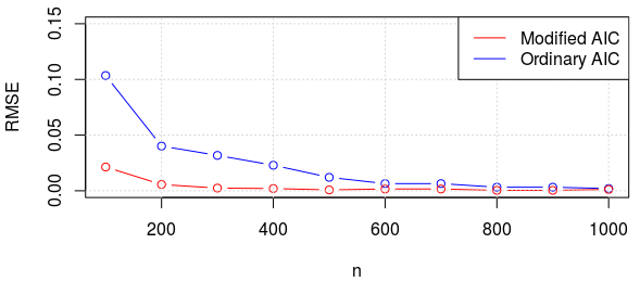
X1,X2,,Xnsubscript𝑋1subscript𝑋2subscript𝑋𝑛X_{1},X_{2},\ldots,X_{n} are generated from Np(0,𝚺)subscript𝑁𝑝0𝚺N_{p}(0,\mathbf{\Sigma}) where 𝚺=diag{λ1,,λk,1,,1}𝚺diagsubscript𝜆1subscript𝜆𝑘11\mathbf{\Sigma}=\text{diag}\{\lambda_{1},\ldots,\lambda_{k},1,\ldots,1\}. After fixing a c𝑐c, n𝑛n and p𝑝p are varied such that p/nc𝑝𝑛𝑐p/n\approx c. We compute the RMSE (by 400400400 replications) for our estimator, for the two different choices of δnsubscript𝛿𝑛\delta_{n}, first one is automatic calibration, and the second one by manual tuning (to get the best performance). We compare both these method for the following two models.

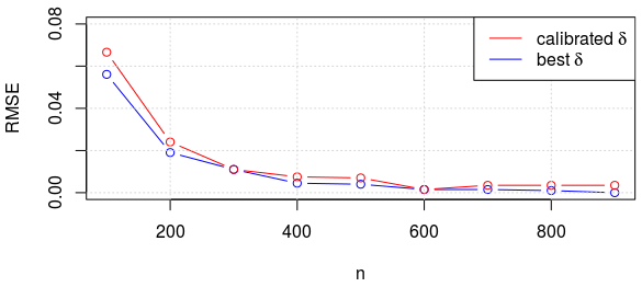
  • Model 1: c=1,k=2,λ1=4.5,λ2=3formulae-sequence𝑐1formulae-sequence𝑘2formulae-sequencesubscript𝜆14.5subscript𝜆23c=1,\,k=2,\,\lambda_{1}=4.5,\lambda_{2}=3. In this case our calibrated δnsubscript𝛿𝑛\delta_{n} has performance really close to the “ideal” δnsubscript𝛿𝑛\delta_{n} as can be seen by the Figure 4-(a).

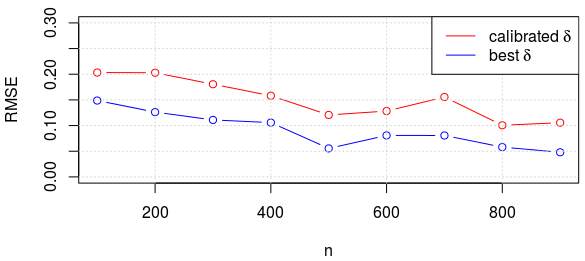
  • Model 2: c=1,k=2,λ1=3,λ2=2.3formulae-sequence𝑐1formulae-sequence𝑘2formulae-sequencesubscript𝜆13subscript𝜆22.3c=1,\,k=2,\,\lambda_{1}=3,\lambda_{2}=2.3. In this case the gap between BBP threshold and λksubscript𝜆𝑘\lambda_{k} is very small (=0.3)absent0.3(=0.3). Here the difference between the two choice of δnsubscript𝛿𝑛\delta_{n} is more prominent. The RMSE corresponding to the “best” δnsubscript𝛿𝑛\delta_{n} is about 25%percent2525\% lower than that of our calibrated δnsubscript𝛿𝑛\delta_{n} (See Figure 4-(b)).

  c=1,k=2,λ1=4.5,λ2=3formulae-sequence𝑐1formulae-sequence𝑘2formulae-sequencesubscript𝜆14.5subscript𝜆23c=1,\,k=2,\,\lambda_{1}=4.5,\lambda_{2}=3   c=1,k=2,λ1=3,λ2=2.3formulae-sequence𝑐1formulae-sequence𝑘2formulae-sequencesubscript𝜆13subscript𝜆22.3c=1,\,k=2,\,\lambda_{1}=3,\lambda_{2}=2.3
Refer to caption Refer to caption
     (a)      (b)
Figure 4: (a) Model 1; (b) Model 2.

The main takeaway here is that when the gap is not too small then our calibrated δnsubscript𝛿𝑛\delta_{n} has performance very close to the “best” δnsubscript𝛿𝑛\delta_{n}, but when the “gap” is very small, further study needs to be done to be able to adaptively choose δnsubscript𝛿𝑛\delta_{n} based on the “gap”. Nevertheless in either case (gap: small/big) our modified AIC criterion (with calibrated δnsubscript𝛿𝑛\delta_{n}) works better than the other estimators in the literature as shown in the next two sections.

4.2 Comparison study I

In this section we compare our modified AIC estimator against the estimator by Passemier and Yao, (2014) (abbreviated as PY), see section 2.3 for details.

X1,X2,,Xnsubscript𝑋1subscript𝑋2subscript𝑋𝑛X_{1},X_{2},\ldots,X_{n} are generated from a p𝑝p-variate Gaussian distribution with mean 0 and a spiked variance-covariance matrix Σ=diag{λ1,,λk,1,,1}Σdiagsubscript𝜆1subscript𝜆𝑘11\Sigma=\text{diag}\{\lambda_{1},\ldots,\lambda_{k},1,\ldots,1\}. After fixing a c𝑐c, n𝑛n and p𝑝p are varied such that p/nc𝑝𝑛𝑐p/n\approx c. We compute the RMSE for our estimator (with calibrated δnsubscript𝛿𝑛\delta_{n}) and for PY estimator (as proposed in their paper with automatic calibration) by conducting 100100100 independent replications. We compare both these method for the following models.

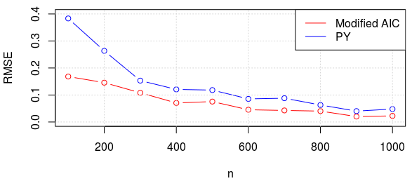
  • Model A: c=1𝑐1c=1, k=2𝑘2k=2, λ1=3.5,λ2=2.5formulae-sequencesubscript𝜆13.5subscript𝜆22.5\lambda_{1}=3.5,\lambda_{2}=2.5. Our method performs uniformly better than PY (see Figure 5-(a)), though the advantage seems to decrease as n𝑛n increases.

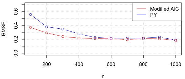
  • Model B: c=1𝑐1c=1, k=2𝑘2k=2, λ1=3,λ2=2.1formulae-sequencesubscript𝜆13subscript𝜆22.1\lambda_{1}=3,\lambda_{2}=2.1. In this case the gap between BBP threshold and λksubscript𝜆𝑘\lambda_{k} is very small (=0.1)absent0.1(=0.1). Our method is still the better one (see Figure 5-(b)).

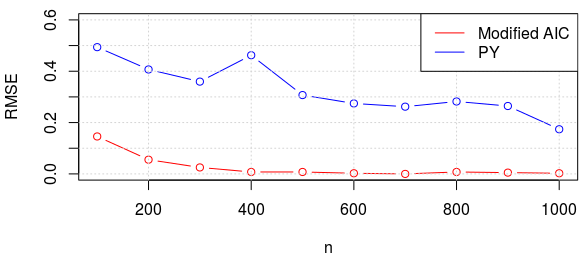
  • Model C: c=1𝑐1c=1, k=2𝑘2k=2, λ1=3,λ2=3formulae-sequencesubscript𝜆13subscript𝜆23\lambda_{1}=3,\lambda_{2}=3 (equal spikes). Our Method is clearly better than PY’s (see Figure 5-(c)) and the advantage gained is significant especially in case of equal spikes.

  c=1𝑐1c=1, k=2𝑘2k=2, λ1=3.5,λ2=2.5formulae-sequencesubscript𝜆13.5subscript𝜆22.5\lambda_{1}=3.5,\lambda_{2}=2.5   c=1𝑐1c=1, k=2𝑘2k=2, λ1=3,λ2=2.1formulae-sequencesubscript𝜆13subscript𝜆22.1\lambda_{1}=3,\lambda_{2}=2.1
Refer to caption Refer to caption
     (a)      (b)
  c=1𝑐1c=1, k=2𝑘2k=2, λ1=3,λ2=3formulae-sequencesubscript𝜆13subscript𝜆23\lambda_{1}=3,\lambda_{2}=3
Refer to caption
     (c)
Figure 5: (a) Model A; (b) Model B; (c) Model (c).

4.3 Comparison study II

In this section we compare our estimator against the ordinary AIC criterion as proposed by Bai et al., (2018), see section 2.2 for details.

X1,X2,,Xnsubscript𝑋1subscript𝑋2subscript𝑋𝑛X_{1},X_{2},\ldots,X_{n} are generated from a p𝑝p-variate Gaussian distribution with mean 0, with spiked variance-covariance matrix Σ=diag{λ1,,λk,1,,1}Σdiagsubscript𝜆1subscript𝜆𝑘11\Sigma=\text{diag}\{\lambda_{1},\ldots,\lambda_{k},1,\ldots,1\}. After fixing a c𝑐c, n𝑛n and p𝑝p are varied such that p/nc𝑝𝑛𝑐p/n\approx c. We compute the RMSE for our estimator (with calibrated δnsubscript𝛿𝑛\delta_{n}) and for ordinary AIC criterion by conducting 100100100 independent replications. We compare both these method for the following models.

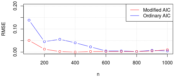
  • Model D: c=1𝑐1c=1, k=2𝑘2k=2 λ1=3.5,λ2=3.5formulae-sequencesubscript𝜆13.5subscript𝜆23.5\lambda_{1}=3.5,\lambda_{2}=3.5. Here λk=λ2subscript𝜆𝑘subscript𝜆2\lambda_{k}=\lambda_{2} is chosen such that it satifies the gap condition (C3) as proposed by Bai et al., (2018). Observe that our method performs uniformly better compared to theirs (see Figure 6-(a)), though the advantage seems to decrease as n𝑛n increases.

  • Model E: c=1𝑐1c=1, k=5𝑘5k=5 λ1=4,λ2=4,λ3=λ4=λ5=3.5formulae-sequencesubscript𝜆14formulae-sequencesubscript𝜆24subscript𝜆3subscript𝜆4subscript𝜆53.5\lambda_{1}=4,\lambda_{2}=4,\lambda_{3}=\lambda_{4}=\lambda_{5}=3.5. Here λk=λ5subscript𝜆𝑘subscript𝜆5\lambda_{k}=\lambda_{5} is chosen such that it satisfies the gap condition (C3). Observe that in this case too our method performs uniformly better compared to theirs (see Figure 6-(b)).

  c=1𝑐1c=1, k=2𝑘2k=2 λ1=3.5,λ2=3.5formulae-sequencesubscript𝜆13.5subscript𝜆23.5\lambda_{1}=3.5,\lambda_{2}=3.5     c=1𝑐1c=1, k=5𝑘5k=5 λ1=4,λ2=4,λ3=λ4=λ5=3.5formulae-sequencesubscript𝜆14formulae-sequencesubscript𝜆24subscript𝜆3subscript𝜆4subscript𝜆53.5\lambda_{1}=4,\lambda_{2}=4,\lambda_{3}=\lambda_{4}=\lambda_{5}=3.5
Refer to caption Refer to caption
     (a)      (b)
Figure 6: (a) Model D; (b) Model E.

4.4 The choice of 𝜹=𝟎𝜹0\boldsymbol{\delta=0}

Observe that we can reach arbitrary close to 1+c1𝑐1+\sqrt{c} , by suitably choosing the penalty term in AIC criterion (α(c)𝛼𝑐\alpha(c)). Motivated by our estimators where we have chosen our gap to be δ𝛿\delta where δ𝛿\delta can be arbitrarily small, or even δn0subscript𝛿𝑛0\delta_{n}\to 0 (in case of weak consistency), we present an estimator where δ𝛿\delta is exactly zero, i.e. choose

α(c)=1cFc(1+c).𝛼𝑐1𝑐subscript𝐹𝑐1𝑐\alpha(c)=\frac{1}{c}F_{c}(1+\sqrt{c}).

We now present a simulation study about this estimator.

  • Simulation setup: c=0.5𝑐0.5c=0.5 is fixed, n𝑛n is varied, X1,X2,,Xnsubscript𝑋1subscript𝑋2subscript𝑋𝑛X_{1},X_{2},\ldots,X_{n} are generated from a p𝑝p-variate Gaussian distribution with mean 00 with spiked variance-covariance matrix (i.e. a diagonal matrix with first k𝑘k entries as 1+c+δ1𝑐𝛿1+\sqrt{c}+\delta and rest pk𝑝𝑘p-k diagonal entries are 1). Here we fixed δ=0.5𝛿0.5\delta=0.5 and k=10𝑘10k=10.

  • Results: We varied n𝑛n from 100100100 to 320032003200 and iterated 505050 times each. Table 2 shows the accuracy (i.e. proportion of times k^^𝑘\hat{k} is equal to true k𝑘k) and the average value of k^^𝑘\hat{k} over 505050 iterations.

    n𝑛n 100 200 400 800 1200 1500 2000 2500 3200
    accuracy 0.02 0.04 0.04 0.26 0.48 0.76 0.94 0.96 0.94
    avg k^^𝑘\hat{k} 5.56 7.08 7.82 8.98 9.50 9.82 10.06 10.00 10.06
    Table 2: The behaviour of our estimator with the choice δ=0𝛿0\delta=0.

The results suggest that the estimator is consistent. We leave the theoretical analysis of this case to future work.

5 Conclusion

In this article, we have considered the AIC cirterion for high dimensional model selection. Bai et al., (2018) have shown strong consistency of AIC under a “gap” condition, requiring more signal than what the BBP threshold demands. We have modified the penalty term in AIC suitably and proposed a criterion that achieves strong consistency under arbitrarily small gap. We have also proposed another modification that achieves weak consistency under exactly zero gap. We have made a detailed empirical study of the performance of the proposed criteria. Furthermore, we have compared our second proposal with the estimator of Passemier and Yao, (2014) which also achieves weak consistency under zero gap.

6 Acknowledgements

This article is based on the Masters dissertation Chakraborty, (2020) of the first author under the supervision of the second and the third authors. The authors thank Professors Gopal K. Basak and Tapas Samanta for their insightful comments. The second author is supported by an INSPIRE Faculty Fellowship, Department of Science and Technology, Government of India.

References

  • Akaike, (1998) Akaike, H. (1998). Information theory and an extension of the maximum likelihood principle. In Selected papers of hirotugu akaike, pages 199–213. Springer.
  • Anderson, (1958) Anderson, T. W. (1958). An introduction to multivariate statistical analysis. Technical report.
  • Bai et al., (2018) Bai, Z., Choi, K. P., Fujikoshi, Y., et al. (2018). Consistency of aic and bic in estimating the number of significant components in high-dimensional principal component analysis. The Annals of Statistics, 46(3):1050–1076.
  • Bai and Yao, (2012) Bai, Z. and Yao, J. (2012). On sample eigenvalues in a generalized spiked population model. Journal of Multivariate Analysis, 106:167–177.
  • Baik et al., (2005) Baik, J., Arous, G. B., Péché, S., et al. (2005). Phase transition of the largest eigenvalue for nonnull complex sample covariance matrices. The Annals of Probability, 33(5):1643–1697.
  • Benaych-Georges et al., (2011) Benaych-Georges, F., Guionnet, A., Maida, M., et al. (2011). Fluctuations of the extreme eigenvalues of finite rank deformations of random matrices. Electronic Journal of Probability, 16:1621–1662.
  • Chakraborty, (2020) Chakraborty, A. (2020). Some Contributions to High Dimensional Principal Component Analysis. Master’s thesis, Indian Statistical Institute, Kolkata.
  • Fujikoshi et al., (2011) Fujikoshi, Y., Ulyanov, V. V., and Shimizu, R. (2011). Multivariate statistics: High-dimensional and large-sample approximations, volume 760. John Wiley & Sons.
  • Hu et al., (2020) Hu, J., Zhang, J., and Zhu, J. (2020). Detection of the number of principal components by extended aic-type method.
  • Johnstone, (2001) Johnstone, I. M. (2001). On the distribution of the largest eigenvalue in principal components analysis. Annals of statistics, pages 295–327.
  • Johnstone and Paul, (2018) Johnstone, I. M. and Paul, D. (2018). Pca in high dimensions: An orientation. Proceedings of the IEEE, 106(8):1277–1292.
  • Jolliffe, (1986) Jolliffe, I. T. (1986). Principal components in regression analysis. In Principal component analysis, pages 129–155. Springer.
  • Kritchman and Nadler, (2009) Kritchman, S. and Nadler, B. (2009). Non-parametric detection of the number of signals: Hypothesis testing and random matrix theory. IEEE Transactions on Signal Processing, 57(10):3930–3941.
  • Li et al., (2019) Li, Z., Han, F., and Yao, J. (2019). Asymptotic joint distribution of extreme eigenvalues and trace of large sample covariance matrix in a generalized spiked population model. arXiv preprint arXiv:1906.09639.
  • Nadler, (2010) Nadler, B. (2010). Nonparametric detection of signals by information theoretic criteria: performance analysis and an improved estimator. IEEE Transactions on Signal Processing, 58(5):2746–2756.
  • Passemier and Yao, (2014) Passemier, D. and Yao, J. (2014). Estimation of the number of spikes, possibly equal, in the high-dimensional case. Journal of Multivariate Analysis, 127:173–183.
  • Paul, (2007) Paul, D. (2007). Asymptotics of sample eigenstructure for a large dimensional spiked covariance model. Statistica Sinica, pages 1617–1642.
  • Schwarz et al., (1978) Schwarz, G. et al. (1978). Estimating the dimension of a model. The annals of statistics, 6(2):461–464.
  • Silverstein, (1995) Silverstein, J. W. (1995). Strong convergence of the empirical distribution of eigenvalues of large dimensional random matrices. Journal of Multivariate Analysis, 55(2):331–339.
  • Wax and Kailath, (1985) Wax, M. and Kailath, T. (1985). Detection of signals by information theoretic criteria. IEEE Transactions on acoustics, speech, and signal processing, 33(2):387–392.

7 Appendix

7.1 Preparatory Lemmas

The proof of Theorem 3.1, 3.3 and 3.4 rely on several additional lemmas which are organised in this section. We first recall a lemma stated earlier in Section 2.1.1 as Lemma 2.1.

Lemma 7.1.

Let lipsubscript𝑙𝑖𝑝l_{ip} denote the ith largest eigenvalue of Snsubscript𝑆𝑛S_{n} the covariance matrix in our setup. Suppose that 𝔼(x114<)𝔼superscriptsubscript𝑥114\mathbb{E}(x_{11}^{4}<\infty), condition (C1)C1(\ref{eq:C1}) and (C2)C2(\ref{eq:C2}) hold, and that λ1subscript𝜆1\lambda_{1} is bounded.

  • (i)

    If λi>1+csubscript𝜆𝑖1𝑐\lambda_{i}>1+\sqrt{c}, then lipa.s.ψi=λi+cλiλi1l_{ip}\overset{a.s.}{\to}\psi_{i}=\lambda_{i}+\frac{c\lambda_{i}}{\lambda_{i}-1}.

  • (ii)

    λi<1+csubscript𝜆𝑖1𝑐\lambda_{i}<1+\sqrt{c} and i/pα𝑖𝑝𝛼i/p\to\alpha, then lipa.s.μ1αl_{ip}\overset{a.s.}{\to}\mu_{1-\alpha}(where μαsubscript𝜇𝛼\mu_{\alpha} is the α𝛼\alpha-quantile of MP distribution). In particular if i is bounded lipa.s.μ1=b:=(1+c)2l_{ip}\overset{a.s.}{\to}\mu_{1}=b:=(1+\sqrt{c})^{2}.

The next lemma is a direct consequence of Theorem 3.1 of, Li et al., (2019).

Lemma 7.2.

Under the given assumptions of the Theorem 3.3 or 3.4 we have that

trace(Sn)trace(V)𝑑N(0,σ02),𝑡𝑟𝑎𝑐𝑒subscript𝑆𝑛𝑡𝑟𝑎𝑐𝑒𝑉𝑑𝑁0superscriptsubscript𝜎02trace(S_{n})-trace(V)\overset{d}{\to}N(0,\sigma_{0}^{2}),

where σ0subscript𝜎0\sigma_{0} is some constant independent of n𝑛n or p𝑝p.

Next lemma is a direct consequence of Proposition 5.85.85.8 from Benaych-Georges et al., (2011).

Lemma 7.3.

Assume that the entries xisuperscript𝑥𝑖x^{i} of x𝑥x have a symmetric law and a sub-exponential decay, that means \exists positive constants C,C𝐶superscript𝐶C,C^{\prime} such that, for all t>C𝑡superscript𝐶t>C^{\prime}, we have (|xi|tC)etsuperscript𝑥𝑖superscript𝑡𝐶superscript𝑒𝑡\mathbb{P}(|x^{i}|\geq t^{C})\leq e^{-t}. Then, for all 1iL1𝑖𝐿1\leq i\leq L with a prefixed range L,

n23(λk+ib)=O(1).superscript𝑛23subscript𝜆𝑘𝑖𝑏subscript𝑂1n^{\frac{2}{3}}(\lambda_{k+i}-b)=O_{\mathbb{P}}(1).

7.2 Weak Consistency Proof

In this section we are going to prove Theorem 3.3 and 3.4.

Proof of the Theorem 3.3. We will show that (k^A=k)1subscriptsuperscript^𝑘absent𝐴𝑘1\mathbb{P}(\hat{k}^{**}_{A}=k)\to 1 as n𝑛n\to\infty. We will show that by breaking the problem into two cases j<k𝑗𝑘j<k and j>k𝑗𝑘j>k, in both these cases we will show that (Aj>Ak)1subscriptsuperscript𝐴absent𝑗subscriptsuperscript𝐴absent𝑘1\mathbb{P}(A^{**}_{j}>A^{**}_{k})\to 1 as n𝑛n\to\infty.
Case I: When j<k𝑗𝑘j<k,

AjAksubscriptsuperscript𝐴absent𝑗subscriptsuperscript𝐴absent𝑘\displaystyle A^{**}_{j}-A^{**}_{k} =i=j+1k(Ai1Ai)absentsuperscriptsubscript𝑖𝑗1𝑘subscriptsuperscript𝐴absent𝑖1subscriptsuperscript𝐴absent𝑖\displaystyle=\sum_{i=j+1}^{k}(A^{**}_{i-1}-A^{**}_{i})
=i=j+1k(pi+1)log{11pi+1(1lipl¯ip)}+logl¯iploglip1p/nFp/n(1+p/n+δn)pi+1nabsentsuperscriptsubscript𝑖𝑗1𝑘𝑝𝑖111𝑝𝑖11subscript𝑙𝑖𝑝subscript¯𝑙𝑖𝑝subscript¯𝑙𝑖𝑝subscript𝑙𝑖𝑝1𝑝𝑛subscript𝐹𝑝𝑛1𝑝𝑛subscript𝛿𝑛𝑝𝑖1𝑛\displaystyle\begin{split}&=\sum_{i=j+1}^{k}(p-i+1)\log\left\{1-\frac{1}{p-i+1}\left(1-\frac{l_{ip}}{\bar{l}_{ip}}\right)\right\}\\ &+\log\bar{l}_{ip}-\log l_{ip}-\frac{1}{p/n}F_{p/n}(1+\sqrt{p/n}+\delta_{n})\frac{p-i+1}{n}\end{split}
a.s.i=j+1kψi1logψiFc(1+c)\displaystyle\overset{a.s.}{\to}\sum_{i=j+1}^{k}\psi_{i}-1-\log\psi_{i}-F_{c}(1+\sqrt{c})
=i=j+1kFc(λi)Fc(1+c)absentsuperscriptsubscript𝑖𝑗1𝑘subscript𝐹𝑐subscript𝜆𝑖subscript𝐹𝑐1𝑐\displaystyle=\sum_{i=j+1}^{k}F_{c}(\lambda_{i})-F_{c}(1+\sqrt{c})

Only step that needs to be justified is the third step , specifically
Claim:

(pi+1)log{11pi+1(1lipl¯ip)}a.s.ψi1.(p-i+1)\log\left\{1-\frac{1}{p-i+1}\left(1-\frac{l_{ip}}{\bar{l}_{ip}}\right)\right\}\overset{a.s.}{\to}\psi_{i}-1.

Observe that, |(pi+1)log{11pi+1(1lipl¯ip)}(ψi1)|𝑝𝑖111𝑝𝑖11subscript𝑙𝑖𝑝subscript¯𝑙𝑖𝑝subscript𝜓𝑖1\left|(p-i+1)\log\left\{1-\frac{1}{p-i+1}\left(1-\frac{l_{ip}}{\bar{l}_{ip}}\right)\right\}-(\psi_{i}-1)\right|
\leq |(pi+1)log{11pi+1(1lipl¯ip)}(1lipl¯ip)|𝑝𝑖111𝑝𝑖11subscript𝑙𝑖𝑝subscript¯𝑙𝑖𝑝1subscript𝑙𝑖𝑝subscript¯𝑙𝑖𝑝\left|-(p-i+1)\log\left\{1-\frac{1}{p-i+1}\left(1-\frac{l_{ip}}{\bar{l}_{ip}}\right)\right\}-\left(1-\frac{l_{ip}}{\bar{l}_{ip}}\right)\right| +|lipl¯ipψi|.subscript𝑙𝑖𝑝subscript¯𝑙𝑖𝑝subscript𝜓𝑖\left|\frac{l_{ip}}{\bar{l}_{ip}}-\psi_{i}\right|.

Result:(Taylor series theorem) For a twice differentiable f𝑓f on (a,b)𝑎𝑏(a,b) with fsuperscript𝑓f^{\prime} continuous on [a,b]𝑎𝑏[a,b]. Assume that c[a,b]𝑐𝑎𝑏c\in[a,b]. Then for every x[a,b]c𝑥𝑎𝑏𝑐x\in[a,b]\neq c, there exists point x1subscript𝑥1x_{1} in (min(x,c),max(x.c))(\min(x,c),\max(x.c)) such that

f(x)=f(c)+f(c)(xc)+f′′(x1)2(xc)2.𝑓𝑥𝑓𝑐superscript𝑓𝑐𝑥𝑐superscript𝑓′′subscript𝑥12superscript𝑥𝑐2f(x)=f(c)+f^{\prime}(c)(x-c)+\frac{f^{\prime\prime}(x_{1})}{2}(x-c)^{2}.

Using the above theorem we get under prescribed conditions on f𝑓f we have

f(x+h0)=f(x)+f(x)h0+f′′(ζ)2h02whereζ(min(x,x+h0),max(x.x+h0)).f(x+h_{0})=f(x)+f^{\prime}(x)h_{0}+\frac{f^{\prime\prime}(\zeta)}{2}h_{0}^{2}\quad where\,\,\zeta\in(\min(x,x+h_{0}),\max(x.x+h_{0})).

Choose

f(x)=log(1x)x=0h0=1pi+1(1lipl¯ip)formulae-sequence𝑓𝑥1𝑥formulae-sequence𝑥0subscript01𝑝𝑖11subscript𝑙𝑖𝑝subscript¯𝑙𝑖𝑝f(x)=\log(1-x)\qquad x=0\qquad h_{0}=\frac{1}{p-i+1}\left(1-\frac{l_{ip}}{\bar{l}_{ip}}\right)

and observe that

f(x)=11xf′′(x)=1(1x)2.formulae-sequencesuperscript𝑓𝑥11𝑥superscript𝑓′′𝑥1superscript1𝑥2f^{\prime}(x)=-\frac{1}{1-x}\qquad f^{\prime\prime}(x)=\frac{1}{(1-x)^{2}}.

We have that

log{11pi+1(1lipl¯ip)}=1pi+1(1lipl¯ip)+h022(1ζ)211𝑝𝑖11subscript𝑙𝑖𝑝subscript¯𝑙𝑖𝑝1𝑝𝑖11subscript𝑙𝑖𝑝subscript¯𝑙𝑖𝑝superscriptsubscript022superscript1𝜁2\log\left\{1-\frac{1}{p-i+1}\left(1-\frac{l_{ip}}{\bar{l}_{ip}}\right)\right\}=-\frac{1}{p-i+1}\left(1-\frac{l_{ip}}{\bar{l}_{ip}}\right)+\frac{h_{0}^{2}}{2(1-\zeta)^{2}}

where ζ(min(0,h0),max(0,h0))𝜁0subscript00subscript0\zeta\in(\min(0,h_{0}),\max(0,h_{0})).
So we have

(pi+1)log{11pi+1(1lipl¯ip)}=(1lipl¯ip)(pi+1)h022(1ζ)2.𝑝𝑖111𝑝𝑖11subscript𝑙𝑖𝑝subscript¯𝑙𝑖𝑝1subscript𝑙𝑖𝑝subscript¯𝑙𝑖𝑝𝑝𝑖1superscriptsubscript022superscript1𝜁2-(p-i+1)\log\left\{1-\frac{1}{p-i+1}\left(1-\frac{l_{ip}}{\bar{l}_{ip}}\right)\right\}=\left(1-\frac{l_{ip}}{\bar{l}_{ip}}\right)-(p-i+1)\frac{h_{0}^{2}}{2(1-\zeta)^{2}}.

Hence

|(pi+1)log{11pi+1(1lipl¯ip)}(1lipl¯ip)|𝑝𝑖111𝑝𝑖11subscript𝑙𝑖𝑝subscript¯𝑙𝑖𝑝1subscript𝑙𝑖𝑝subscript¯𝑙𝑖𝑝\displaystyle\left|-(p-i+1)\log\left\{1-\frac{1}{p-i+1}\left(1-\frac{l_{ip}}{\bar{l}_{ip}}\right)\right\}-\left(1-\frac{l_{ip}}{\bar{l}_{ip}}\right)\right| =|(pi+1)h022(1ζ)2|absent𝑝𝑖1superscriptsubscript022superscript1𝜁2\displaystyle=\left|(p-i+1)\frac{h_{0}^{2}}{2(1-\zeta)^{2}}\right|
=\displaystyle= 1(1ζ)2(1lipl¯ip)21pi+11superscript1𝜁2superscript1subscript𝑙𝑖𝑝subscript¯𝑙𝑖𝑝21𝑝𝑖1\displaystyle\frac{1}{(1-\zeta)^{2}}\left(1-\frac{l_{ip}}{\bar{l}_{ip}}\right)^{2}\frac{1}{p-i+1}

Lets look at the R.H.S, we know from Lemma 2.1 that lipa.s.ψil_{ip}\overset{a.s.}{\to}\psi_{i} and from the MP-law that l¯ipa.s.μMP=1\bar{l}_{ip}\overset{a.s.}{\to}\mu_{MP}=1, where μMPsubscript𝜇𝑀𝑃\mu_{MP} is the mean of the MP distribution.
Using these we infer that

(1lipl¯ip)2a.s(1ψi)2&h0=1pi+1(1lipl¯ip)a.s0.superscript1subscript𝑙𝑖𝑝subscript¯𝑙𝑖𝑝2formulae-sequence𝑎𝑠superscript1subscript𝜓𝑖2subscript01𝑝𝑖11subscript𝑙𝑖𝑝subscript¯𝑙𝑖𝑝formulae-sequence𝑎𝑠0\left(1-\frac{l_{ip}}{\bar{l}_{ip}}\right)^{2}\overset{a.s}{\to}(1-\psi_{i})^{2}\quad\&\quad h_{0}=\frac{1}{p-i+1}\left(1-\frac{l_{ip}}{\bar{l}_{ip}}\right)\overset{a.s}{\to}0.

Now using sandwich theorem we have that ζa.s0𝜁formulae-sequence𝑎𝑠0\zeta\overset{a.s}{\to}0 as ζ(min(0,h0),max(0,h0))𝜁0subscript00subscript0\zeta\in(\min(0,h_{0}),\max(0,h_{0})) so, we have that 1(1ζ)2a.s11superscript1𝜁2formulae-sequence𝑎𝑠1\frac{1}{(1-\zeta)^{2}}\overset{a.s}{\to}1.
Therefore,

1(1ζ)2(1lipl¯ip)2a.s(1ψi)2.1superscript1𝜁2superscript1subscript𝑙𝑖𝑝subscript¯𝑙𝑖𝑝2formulae-sequence𝑎𝑠superscript1subscript𝜓𝑖2\frac{1}{(1-\zeta)^{2}}\left(1-\frac{l_{ip}}{\bar{l}_{ip}}\right)^{2}\overset{a.s}{\to}(1-\psi_{i})^{2}.

So,

|(pi+1)log{11pi+1(1lipl¯ip)}(1lipl¯ip)|=(1lipl¯ip)2(1ζ)21pi+1𝑝𝑖111𝑝𝑖11subscript𝑙𝑖𝑝subscript¯𝑙𝑖𝑝1subscript𝑙𝑖𝑝subscript¯𝑙𝑖𝑝superscript1subscript𝑙𝑖𝑝subscript¯𝑙𝑖𝑝2superscript1𝜁21𝑝𝑖1\left|-(p-i+1)\log\left\{1-\frac{1}{p-i+1}\left(1-\frac{l_{ip}}{\bar{l}_{ip}}\right)\right\}-\left(1-\frac{l_{ip}}{\bar{l}_{ip}}\right)\right|=\frac{\left(1-\frac{l_{ip}}{\bar{l}_{ip}}\right)^{2}}{(1-\zeta)^{2}}\frac{1}{p-i+1}

As 1pi+101𝑝𝑖10\frac{1}{p-i+1}\to 0 coupled with previous fact, we can conclude that

|(pi+1)log{11pi+1(1lipl¯ip)}(1lipl¯ip)|a.s.0.\left|-(p-i+1)\log\left\{1-\frac{1}{p-i+1}\left(1-\frac{l_{ip}}{\bar{l}_{ip}}\right)\right\}-\left(1-\frac{l_{ip}}{\bar{l}_{ip}}\right)\right|\overset{a.s.}{\to}0.

Next using Lemma 2.1 observe that lipa.s.ψil_{ip}\overset{a.s.}{\to}\psi_{i} and l¯ipa.s.1\bar{l}_{ip}\overset{a.s.}{\to}1 which implies that

lipl¯ipa.s.ψi|lipl¯ipψi|a.s.0.\frac{l_{ip}}{\bar{l}_{ip}}\overset{a.s.}{\to}\psi_{i}\implies\left|\frac{l_{ip}}{\bar{l}_{ip}}-\psi_{i}\right|\overset{a.s.}{\to}0.

Hence the claim is proved.

Next using the monotonicity of Fc(.)F_{c}(.) and λisubscript𝜆𝑖\lambda_{i}’s we have

AjAka.s.i=j+1kFc(λi)Fc(1+c)>(kj)[Fc(λk)Fc(1+c)].A^{**}_{j}-A^{**}_{k}\overset{a.s.}{\to}\sum_{i=j+1}^{k}F_{c}(\lambda_{i})-F_{c}(1+\sqrt{c})>(k-j)[F_{c}(\lambda_{k})-F_{c}(1+\sqrt{c})].

We know that λk>1+csubscript𝜆𝑘1𝑐\lambda_{k}>1+\sqrt{c} so we have that Fc(λk)Fc(1+c)>0subscript𝐹𝑐subscript𝜆𝑘subscript𝐹𝑐1𝑐0F_{c}(\lambda_{k})-F_{c}(1+\sqrt{c})>0 hence (limn(AjAk)>0)=1subscript𝑛subscriptsuperscript𝐴absent𝑗subscriptsuperscript𝐴absent𝑘01\mathbb{P}(\lim_{n\to\infty}(A^{**}_{j}-A^{**}_{k})>0)=1 j<kfor-all𝑗𝑘\forall j<k this implies that (limnk^Ak)=1subscript𝑛subscriptsuperscript^𝑘absent𝐴𝑘1\mathbb{P}(\lim_{n\to\infty}\hat{k}^{**}_{A}\geq k)=1 or a weaker condition that (k^Ak)n1subscriptsuperscript^𝑘absent𝐴𝑘𝑛1\mathbb{P}(\hat{k}^{**}_{A}\geq k)\overset{n\to\infty}{\to}1.

Case II: When j>k𝑗𝑘j>k and j𝑗j is bounded, i.e. j<s𝑗𝑠j<s,

AjAksubscriptsuperscript𝐴absent𝑗subscriptsuperscript𝐴absent𝑘\displaystyle A^{**}_{j}-A^{**}_{k} =i=k+1j(AiAi1)absentsuperscriptsubscript𝑖𝑘1𝑗subscriptsuperscript𝐴absent𝑖subscriptsuperscript𝐴absent𝑖1\displaystyle=\sum_{i=k+1}^{j}(A^{**}_{i}-A^{**}_{i-1})
=i=k+1j(pi+1)log{11pi+1(1lipl¯ip)}logl¯ip+loglip+1p/nFp/n(1+p/n+δn)pi+1nabsentsuperscriptsubscript𝑖𝑘1𝑗𝑝𝑖111𝑝𝑖11subscript𝑙𝑖𝑝subscript¯𝑙𝑖𝑝subscript¯𝑙𝑖𝑝subscript𝑙𝑖𝑝1𝑝𝑛subscript𝐹𝑝𝑛1𝑝𝑛subscript𝛿𝑛𝑝𝑖1𝑛\displaystyle\begin{split}&=\sum_{i=k+1}^{j}-(p-i+1)\log\left\{1-\frac{1}{p-i+1}\left(1-\frac{l_{ip}}{\bar{l}_{ip}}\right)\right\}\\ &-\log\bar{l}_{ip}+\log l_{ip}+\frac{1}{p/n}F_{p/n}(1+\sqrt{p/n}+\delta_{n})\frac{p-i+1}{n}\end{split}

Lets look at hn2/3(AjAk)superscript𝑛23subscriptsuperscript𝐴absent𝑗subscriptsuperscript𝐴absent𝑘hn^{2/3}(A^{**}_{j}-A^{**}_{k}) where h00h\to 0 as n𝑛n\to\infty, pick the ith𝑖𝑡ith term, we divide the expression into sum of four parts as follows

  1. 1.

    hn2/3logl¯ipsuperscript𝑛23subscript¯𝑙𝑖𝑝-hn^{2/3}\log\bar{l}_{ip}

  2. 2.

    hn2/3(logliplogb)superscript𝑛23subscript𝑙𝑖𝑝𝑏hn^{2/3}(\log l_{ip}-\log b)

  3. 3.

    hn2/3[(pi+1)log{11pi+1(1lipl¯ip)}(1b)]superscript𝑛23delimited-[]𝑝𝑖111𝑝𝑖11subscript𝑙𝑖𝑝subscript¯𝑙𝑖𝑝1𝑏hn^{2/3}\left[-(p-i+1)\log\left\{1-\frac{1}{p-i+1}\left(1-\frac{l_{ip}}{\bar{l}_{ip}}\right)\right\}-(1-b)\right]

  4. 4.

    hn2/3(1p/nFp/n(1+p/n+δn)pi+1n+logb+1b)superscript𝑛231𝑝𝑛subscript𝐹𝑝𝑛1𝑝𝑛subscript𝛿𝑛𝑝𝑖1𝑛𝑏1𝑏hn^{2/3}\left(\frac{1}{p/n}F_{p/n}(1+\sqrt{p/n}+\delta_{n})\frac{p-i+1}{n}+\log b+1-b\right)

Here b:=ψc(1+c)=(1+c)2assign𝑏subscript𝜓𝑐1𝑐superscript1𝑐2b:=\psi_{c}(1+\sqrt{c})=(1+\sqrt{c})^{2}.
Let us begin analysing each of these terms one by one

  1. 1.

    hn2/3logl¯ipsuperscript𝑛23subscript¯𝑙𝑖𝑝-hn^{2/3}\log\bar{l}_{ip}
    Using Lemma 7.2:

    trace(Sn)trace(Σp)N(0,σ02)𝑡𝑟𝑎𝑐𝑒subscript𝑆𝑛𝑡𝑟𝑎𝑐𝑒subscriptΣ𝑝𝑁0superscriptsubscript𝜎02trace(S_{n})-trace(\Sigma_{p})\to N(0,\sigma_{0}^{2})

    \implies p(j=1pljppj=1pλjp)=Op(1)𝑝superscriptsubscript𝑗1𝑝subscript𝑙𝑗𝑝𝑝superscriptsubscript𝑗1𝑝subscript𝜆𝑗𝑝subscript𝑂𝑝1p(\frac{\sum_{j=1}^{p}l_{jp}}{p}-\frac{\sum_{j=1}^{p}\lambda_{j}}{p})=O_{p}(1)
    \implies p(j=1iljp+j=i+1pljppj=1iλj+(pi)p)=Op(1)𝑝superscriptsubscript𝑗1𝑖subscript𝑙𝑗𝑝superscriptsubscript𝑗𝑖1𝑝subscript𝑙𝑗𝑝𝑝superscriptsubscript𝑗1𝑖subscript𝜆𝑗𝑝𝑖𝑝subscript𝑂𝑝1p(\frac{\sum_{j=1}^{i}l_{jp}+\sum_{j=i+1}^{p}l_{jp}}{p}-\frac{\sum_{j=1}^{i}\lambda_{j}+(p-i)}{p})=O_{p}(1)
    \implies p((pip)[l¯ip1]+j=1kljpj=1kλjp+j=k+1i(ljpλj)p))=Op(1)p\left((\frac{p-i}{p})[\bar{l}_{ip}-1]+\frac{\sum_{j=1}^{k}l_{jp}-\sum_{j=1}^{k}\lambda_{j}}{p}+\frac{\sum_{j=k+1}^{i}(l_{jp}-\lambda_{j})}{p})\right)=O_{p}(1)
    \implies (pi)[l¯ip1]+j=1k(ljpλj)+j=k+1i(ljp1)=Op(1)𝑝𝑖delimited-[]subscript¯𝑙𝑖𝑝1superscriptsubscript𝑗1𝑘subscript𝑙𝑗𝑝subscript𝜆𝑗superscriptsubscript𝑗𝑘1𝑖subscript𝑙𝑗𝑝1subscript𝑂𝑝1(p-i)[\bar{l}_{ip}-1]+\sum_{j=1}^{k}(l_{jp}-\lambda_{j})+\sum_{j=k+1}^{i}(l_{jp}-1)=O_{p}(1)

    We know that ljpψj=ψc(λj)subscript𝑙𝑗𝑝subscript𝜓𝑗subscript𝜓𝑐subscript𝜆𝑗l_{jp}\to\psi_{j}=\psi_{c}(\lambda_{j}) a.s.formulae-sequence𝑎𝑠a.s. if jk𝑗𝑘j\leq k otherwise ljpbsubscript𝑙𝑗𝑝𝑏l_{jp}\to b a.s.formulae-sequence𝑎𝑠a.s. when j>k𝑗𝑘j>k and j𝑗j is finite.

    j=1k(ljpλj)+j=k+1i(ljp1)a.s.j=1k(ψjλj)+(ik)(b1).\sum_{j=1}^{k}(l_{jp}-\lambda_{j})+\sum_{j=k+1}^{i}(l_{jp}-1)\overset{a.s.}{\to}\sum_{j=1}^{k}(\psi_{j}-\lambda_{j})+(i-k)(b-1).

    This along with the previous fact implies that

    (pi)[l¯ip1]=Op(1).𝑝𝑖delimited-[]subscript¯𝑙𝑖𝑝1subscript𝑂𝑝1(p-i)[\bar{l}_{ip}-1]=O_{p}(1).

    So

    hn2/3[l¯ip1]=hn2/3pi(pi)[l¯ip1],superscript𝑛23delimited-[]subscript¯𝑙𝑖𝑝1superscript𝑛23𝑝𝑖𝑝𝑖delimited-[]subscript¯𝑙𝑖𝑝1hn^{2/3}[\bar{l}_{ip}-1]=\frac{hn^{2/3}}{p-i}(p-i)[\bar{l}_{ip}-1],

    coupled with the fact that p/nc>0𝑝𝑛𝑐0p/n\to c>0 and Slutsky’s theorem we have that

    hn2/3[l¯ip1]𝑝0.superscript𝑛23delimited-[]subscript¯𝑙𝑖𝑝1𝑝0hn^{2/3}[\bar{l}_{ip}-1]\overset{p}{\to}0.

    Next by mean value theorem we have that:

    logxlog1=1ζ(x)(x1) where min(1,x)<ζ(x)<max(1,x).formulae-sequence𝑥11𝜁𝑥𝑥1 where 1𝑥𝜁𝑥1𝑥\log x-\log 1=\frac{1}{\zeta(x)}(x-1)\qquad\text{ where }\min(1,x)<\zeta(x)<\max(1,x).

    Using the above we can infer that

    hn2/3logl¯ip=hn2/3ζ(l¯ip)(l¯ip1).superscript𝑛23subscript¯𝑙𝑖𝑝superscript𝑛23𝜁subscript¯𝑙𝑖𝑝subscript¯𝑙𝑖𝑝1hn^{2/3}\log\bar{l}_{ip}=\frac{hn^{2/3}}{\zeta(\bar{l}_{ip})}(\bar{l}_{ip}-1).

    As l¯ip𝑝1subscript¯𝑙𝑖𝑝𝑝1\bar{l}_{ip}\overset{p}{\to}1. Using sandwich theorem we have:

    ζ(l¯ip)𝑝1.𝜁subscript¯𝑙𝑖𝑝𝑝1\zeta(\bar{l}_{ip})\overset{p}{\to}1.

    Therefore using Slutsky’s Theorem we have that:

    hn2/3logl¯ip=hn2/3ζ(l¯ip)(l¯ip1)𝑝0.superscript𝑛23subscript¯𝑙𝑖𝑝superscript𝑛23𝜁subscript¯𝑙𝑖𝑝subscript¯𝑙𝑖𝑝1𝑝0-hn^{2/3}\log\bar{l}_{ip}=-\frac{hn^{2/3}}{\zeta(\bar{l}_{ip})}(\bar{l}_{ip}-1)\overset{p}{\to}0.
  2. 2.

    hn2/3(logliplogb)superscript𝑛23subscript𝑙𝑖𝑝𝑏hn^{2/3}(\log l_{ip}-\log b)
    By mean value theorem we have that:

    logxlogb=1ζ(x)(xb) where min(b,x)<ζ(x)<max(b,x).formulae-sequence𝑥𝑏1𝜁𝑥𝑥𝑏 where 𝑏𝑥𝜁𝑥𝑏𝑥\log x-\log b=\frac{1}{\zeta(x)}(x-b)\qquad\text{ where }\min(b,x)<\zeta(x)<\max(b,x).

    Therefore

    logliplogb=1ζ(lip)(lipb).subscript𝑙𝑖𝑝𝑏1𝜁subscript𝑙𝑖𝑝subscript𝑙𝑖𝑝𝑏\log l_{ip}-\log b=\frac{1}{\zeta(l_{ip})}(l_{ip}-b).

    Using Lemma 7.3

    n2/3(lipb)=Op(1)k<is.formulae-sequencesuperscript𝑛23subscript𝑙𝑖𝑝𝑏subscript𝑂𝑝1for-all𝑘𝑖𝑠n^{2/3}(l_{ip}-b)=O_{p}(1)\quad\forall k<i\leq s.

    Also as lipa.s.bl_{ip}\overset{a.s.}{\to}b so using sandwich theorem we have ζ(lip)a.s.b\zeta(l_{ip})\overset{a.s.}{\to}b. Therefore we have that:

    hn2/3(logliplogb)=hn2/3(lipb)1ζ(lip),superscript𝑛23subscript𝑙𝑖𝑝𝑏superscript𝑛23subscript𝑙𝑖𝑝𝑏1𝜁subscript𝑙𝑖𝑝hn^{2/3}(\log l_{ip}-\log b)=hn^{2/3}(l_{ip}-b)\frac{1}{\zeta(l_{ip})},

    so using the above fact we have that

    hn2/3(lipb)𝑝,0superscript𝑛23subscript𝑙𝑖𝑝𝑏𝑝0hn^{2/3}(l_{ip}-b)\overset{p}{\to},0

    which implies

    hn2/3(logliplogb)𝑝0.superscript𝑛23subscript𝑙𝑖𝑝𝑏𝑝0hn^{2/3}(\log l_{ip}-\log b)\overset{p}{\to}0.
  3. 3.

    hn2/3[(pi+1)log{11pi+1(1lipl¯ip)}(1b)]superscript𝑛23delimited-[]𝑝𝑖111𝑝𝑖11subscript𝑙𝑖𝑝subscript¯𝑙𝑖𝑝1𝑏hn^{2/3}\left[-(p-i+1)\log\left\{1-\frac{1}{p-i+1}\left(1-\frac{l_{ip}}{\bar{l}_{ip}}\right)\right\}-(1-b)\right]

    Observe that, hn2/3|(pi+1)log{11pi+1(1lipl¯ip)}(1b)|superscript𝑛23𝑝𝑖111𝑝𝑖11subscript𝑙𝑖𝑝subscript¯𝑙𝑖𝑝1𝑏hn^{2/3}\left|-(p-i+1)\log\left\{1-\frac{1}{p-i+1}\left(1-\frac{l_{ip}}{\bar{l}_{ip}}\right)\right\}-(1-b)\right|
    \leq hn2/3|(pi+1)log{11pi+1(1lipl¯ip)}(1lipl¯ip)|superscript𝑛23𝑝𝑖111𝑝𝑖11subscript𝑙𝑖𝑝subscript¯𝑙𝑖𝑝1subscript𝑙𝑖𝑝subscript¯𝑙𝑖𝑝hn^{2/3}\left|-(p-i+1)\log\left\{1-\frac{1}{p-i+1}\left(1-\frac{l_{ip}}{\bar{l}_{ip}}\right)\right\}-\left(1-\frac{l_{ip}}{\bar{l}_{ip}}\right)\right| +|lipl¯ipb|.subscript𝑙𝑖𝑝subscript¯𝑙𝑖𝑝𝑏\left|\frac{l_{ip}}{\bar{l}_{ip}}-b\right|.

    Using the taylors series theorem we get under some conditions on f𝑓f we have

    f(x+h0)=f(x)+f(x)h0+f′′(ζ)2h02ζ(min(x,x+h0),max(x.x+h0))).f(x+h_{0})=f(x)+f^{\prime}(x)h_{0}+\frac{f^{\prime\prime}(\zeta)}{2}h_{0}^{2}\quad\zeta\in(\min(x,x+h_{0}),\max(x.x+h_{0}))).

    Choose

    f(x)=log(1x)x=0h0=1pi+1(1lipl¯ip)formulae-sequence𝑓𝑥1𝑥formulae-sequence𝑥0subscript01𝑝𝑖11subscript𝑙𝑖𝑝subscript¯𝑙𝑖𝑝f(x)=\log(1-x)\qquad x=0\qquad h_{0}=\frac{1}{p-i+1}\left(1-\frac{l_{ip}}{\bar{l}_{ip}}\right)

    As in case I we finally have that

    log{11pi+1(1lipl¯ip)}=1pi+1(1lipl¯ip)+h022(1ζ)211𝑝𝑖11subscript𝑙𝑖𝑝subscript¯𝑙𝑖𝑝1𝑝𝑖11subscript𝑙𝑖𝑝subscript¯𝑙𝑖𝑝superscriptsubscript022superscript1𝜁2\log\left\{1-\frac{1}{p-i+1}\left(1-\frac{l_{ip}}{\bar{l}_{ip}}\right)\right\}=-\frac{1}{p-i+1}\left(1-\frac{l_{ip}}{\bar{l}_{ip}}\right)+\frac{h_{0}^{2}}{2(1-\zeta)^{2}}

    where ζ(min(0,h0),max(0,h0))𝜁0subscript00subscript0\zeta\in(\min(0,h_{0}),\max(0,h_{0}))
    So we have that

    |(pi+1)log{11pi+1(1lipl¯ip)}(1lipl¯ip)|=|(pi+1)h022(1ζ)2|𝑝𝑖111𝑝𝑖11subscript𝑙𝑖𝑝subscript¯𝑙𝑖𝑝1subscript𝑙𝑖𝑝subscript¯𝑙𝑖𝑝𝑝𝑖1superscriptsubscript022superscript1𝜁2\displaystyle\left|-(p-i+1)\log\left\{1-\frac{1}{p-i+1}\left(1-\frac{l_{ip}}{\bar{l}_{ip}}\right)\right\}-\left(1-\frac{l_{ip}}{\bar{l}_{ip}}\right)\right|=\left|(p-i+1)\frac{h_{0}^{2}}{2(1-\zeta)^{2}}\right|

    Which is equal to

    1(1ζ)2(1lipl¯ip)21pi+1.1superscript1𝜁2superscript1subscript𝑙𝑖𝑝subscript¯𝑙𝑖𝑝21𝑝𝑖1\frac{1}{(1-\zeta)^{2}}\left(1-\frac{l_{ip}}{\bar{l}_{ip}}\right)^{2}\frac{1}{p-i+1}.

    Lets look at the R.H.S, we already know that lipa.s.bl_{ip}\overset{a.s.}{\to}b and l¯ipa.s.1.\bar{l}_{ip}\overset{a.s.}{\to}1.
    Using these we infer that

    (1lipl¯ip)2a.s(1b)2&h=1pi+1(1lipl¯ip)a.s0.superscript1subscript𝑙𝑖𝑝subscript¯𝑙𝑖𝑝2formulae-sequence𝑎𝑠superscript1𝑏21𝑝𝑖11subscript𝑙𝑖𝑝subscript¯𝑙𝑖𝑝formulae-sequence𝑎𝑠0\left(1-\frac{l_{ip}}{\bar{l}_{ip}}\right)^{2}\overset{a.s}{\to}(1-b)^{2}\quad\&\quad h=\frac{1}{p-i+1}\left(1-\frac{l_{ip}}{\bar{l}_{ip}}\right)\overset{a.s}{\to}0.

    Now using sandwich theorem we have that ζa.s0𝜁formulae-sequence𝑎𝑠0\zeta\overset{a.s}{\to}0 as ζ(min(0,h0),max(0,h0))𝜁0subscript00subscript0\zeta\in(\min(0,h_{0}),\max(0,h_{0})) so, we have that 1(1ζ)2a.s11superscript1𝜁2formulae-sequence𝑎𝑠1\frac{1}{(1-\zeta)^{2}}\overset{a.s}{\to}1.
    Therefore,

    1(1ζ)2(1lipl¯ip)2a.s(1b)2.1superscript1𝜁2superscript1subscript𝑙𝑖𝑝subscript¯𝑙𝑖𝑝2formulae-sequence𝑎𝑠superscript1𝑏2\frac{1}{(1-\zeta)^{2}}\left(1-\frac{l_{ip}}{\bar{l}_{ip}}\right)^{2}\overset{a.s}{\to}(1-b)^{2}.

    So,

    hn2/3|(pi+1)log{11pi+1(1lipl¯ip)}(1lipl¯ip)|=(1lipl¯ip)2(1ζ)2hn2/3pi+1.superscript𝑛23𝑝𝑖111𝑝𝑖11subscript𝑙𝑖𝑝subscript¯𝑙𝑖𝑝1subscript𝑙𝑖𝑝subscript¯𝑙𝑖𝑝superscript1subscript𝑙𝑖𝑝subscript¯𝑙𝑖𝑝2superscript1𝜁2superscript𝑛23𝑝𝑖1hn^{2/3}\left|-(p-i+1)\log\left\{1-\frac{1}{p-i+1}\left(1-\frac{l_{ip}}{\bar{l}_{ip}}\right)\right\}-\left(1-\frac{l_{ip}}{\bar{l}_{ip}}\right)\right|=\frac{\left(1-\frac{l_{ip}}{\bar{l}_{ip}}\right)^{2}}{(1-\zeta)^{2}}\frac{hn^{2/3}}{p-i+1}.

    As hn2/3pi+10superscript𝑛23𝑝𝑖10\frac{hn^{2/3}}{p-i+1}\to 0 coupled with previous fact, we can conclude that

    hn2/3|(pi+1)log{11pi+1(1lipl¯ip)}(1lipl¯ip)|𝑃0.superscript𝑛23𝑝𝑖111𝑝𝑖11subscript𝑙𝑖𝑝subscript¯𝑙𝑖𝑝1subscript𝑙𝑖𝑝subscript¯𝑙𝑖𝑝𝑃0hn^{2/3}\left|-(p-i+1)\log\left\{1-\frac{1}{p-i+1}\left(1-\frac{l_{ip}}{\bar{l}_{ip}}\right)\right\}-\left(1-\frac{l_{ip}}{\bar{l}_{ip}}\right)\right|\overset{P}{\to}0.

    Next let us deal with

    hn2/3|lipl¯ipb|superscript𝑛23subscript𝑙𝑖𝑝subscript¯𝑙𝑖𝑝𝑏\displaystyle hn^{2/3}\left|\frac{l_{ip}}{\bar{l}_{ip}}-b\right| =hn2/3|lipl¯ipbl¯ip+bl¯ipb|absentsuperscript𝑛23subscript𝑙𝑖𝑝subscript¯𝑙𝑖𝑝𝑏subscript¯𝑙𝑖𝑝𝑏subscript¯𝑙𝑖𝑝𝑏\displaystyle=hn^{2/3}\left|\frac{l_{ip}}{\bar{l}_{ip}}-\frac{b}{\bar{l}_{ip}}+\frac{b}{\bar{l}_{ip}}-b\right|
    hn2/3|lipl¯ipbl¯ip|+hn2/3|bl¯ipb|absentsuperscript𝑛23subscript𝑙𝑖𝑝subscript¯𝑙𝑖𝑝𝑏subscript¯𝑙𝑖𝑝superscript𝑛23𝑏subscript¯𝑙𝑖𝑝𝑏\displaystyle\leq hn^{2/3}\left|\frac{l_{ip}}{\bar{l}_{ip}}-\frac{b}{\bar{l}_{ip}}\right|+hn^{2/3}\left|\frac{b}{\bar{l}_{ip}}-b\right|
    hn2/3|lipb||l¯ip|+hn2/3b|l¯ip1||l¯ip|absentsuperscript𝑛23subscript𝑙𝑖𝑝𝑏subscript¯𝑙𝑖𝑝superscript𝑛23𝑏subscript¯𝑙𝑖𝑝1subscript¯𝑙𝑖𝑝\displaystyle\leq hn^{2/3}\frac{|l_{ip}-b|}{|\bar{l}_{ip}|}+hn^{2/3}b\frac{|\bar{l}_{ip}-1|}{|\bar{l}_{ip}|}

    Using Lemma 7.3

    n2/3(lipb)=Op(1)k<isformulae-sequencesuperscript𝑛23subscript𝑙𝑖𝑝𝑏subscript𝑂𝑝1for-all𝑘𝑖𝑠n^{2/3}(l_{ip}-b)=O_{p}(1)\quad\forall k<i\leq s

    Therefore

    hn2/3(lipb)𝑃0&l¯ipa.s.1hn2/3|lipb||l¯ip|𝑃0.hn^{2/3}(l_{ip}-b)\overset{P}{\to}0\quad\&\quad\bar{l}_{ip}\overset{a.s.}{\to}1\implies hn^{2/3}\frac{|l_{ip}-b|}{|\bar{l}_{ip}|}\overset{P}{\to}0.

    We have already observed that

    hn2/3[l¯ip1]𝑝0superscript𝑛23delimited-[]subscript¯𝑙𝑖𝑝1𝑝0hn^{2/3}[\bar{l}_{ip}-1]\overset{p}{\to}0

    Therefore

    hn2/3[l¯ip1]𝑝0&l¯ipa.s.1bhn2/3|lip1||l¯ip|𝑃0.hn^{2/3}[\bar{l}_{ip}-1]\overset{p}{\to}0\quad\&\quad\bar{l}_{ip}\overset{a.s.}{\to}1\implies bhn^{2/3}\frac{|l_{ip}-1|}{|\bar{l}_{ip}|}\overset{P}{\to}0.

    Hence

    hn2/3|lipl¯ipb|𝑃0.superscript𝑛23subscript𝑙𝑖𝑝subscript¯𝑙𝑖𝑝𝑏𝑃0hn^{2/3}\left|\frac{l_{ip}}{\bar{l}_{ip}}-b\right|\overset{P}{\to}0.

    So finally we have that

    hn2/3[(pi+1)log{11pi+1(1lipl¯ip)}(1b)]𝑃0.superscript𝑛23delimited-[]𝑝𝑖111𝑝𝑖11subscript𝑙𝑖𝑝subscript¯𝑙𝑖𝑝1𝑏𝑃0hn^{2/3}\left[-(p-i+1)\log\left\{1-\frac{1}{p-i+1}\left(1-\frac{l_{ip}}{\bar{l}_{ip}}\right)\right\}-(1-b)\right]\overset{P}{\to}0.
  4. 4.

    Looking at the last term

    hn2/3(1p/nFp/n(1+p/n+δn)pi+1n+logb+1b)superscript𝑛231𝑝𝑛subscript𝐹𝑝𝑛1𝑝𝑛subscript𝛿𝑛𝑝𝑖1𝑛𝑏1𝑏hn^{2/3}\left(\frac{1}{p/n}F_{p/n}(1+\sqrt{p/n}+\delta_{n})\frac{p-i+1}{n}+\log b+1-b\right)

    Call

    α(p,n)=1p/nFp/n(1+p/n+δn)&α(c)=1cFc(1+c)formulae-sequence𝛼𝑝𝑛1𝑝𝑛subscript𝐹𝑝𝑛1𝑝𝑛subscript𝛿𝑛𝛼𝑐1𝑐subscript𝐹𝑐1𝑐\alpha(p,n)=\frac{1}{p/n}F_{p/n}(1+\sqrt{p/n}+\delta_{n})\quad\&\quad\alpha(c)=\frac{1}{c}F_{c}(1+\sqrt{c})

    therefore the last term can be written as

    hn2/3(α(p,n)pn+logb+1b)hn2/3α(p,n)i1n.superscript𝑛23𝛼𝑝𝑛𝑝𝑛𝑏1𝑏superscript𝑛23𝛼𝑝𝑛𝑖1𝑛\displaystyle hn^{2/3}\left(\alpha(p,n)\frac{p}{n}+\log b+1-b\right)-hn^{2/3}\alpha(p,n)\frac{i-1}{n}.

    Observe that

    hn2/3i1n0&α(p,n)α(c)hn2/3α(p,n)i1n0formulae-sequencesuperscript𝑛23𝑖1𝑛0𝛼𝑝𝑛𝛼𝑐superscript𝑛23𝛼𝑝𝑛𝑖1𝑛0hn^{2/3}\frac{i-1}{n}\to 0\quad\&\quad\alpha(p,n)\to\alpha(c)\implies hn^{2/3}\alpha(p,n)\frac{i-1}{n}\to 0

    Therefore asymptotically only the first term matters, which is

    hn2/3(α(p,n)pn+logb+1b)=hn2/3(Fp/n(1+p/n+δn)Fc(1+c)).superscript𝑛23𝛼𝑝𝑛𝑝𝑛𝑏1𝑏superscript𝑛23subscript𝐹𝑝𝑛1𝑝𝑛subscript𝛿𝑛subscript𝐹𝑐1𝑐hn^{2/3}\left(\alpha(p,n)\frac{p}{n}+\log b+1-b\right)=hn^{2/3}\left(F_{p/n}(1+\sqrt{p/n}+\delta_{n})-F_{c}(1+\sqrt{c})\right).

    Now δnsubscript𝛿𝑛\delta_{n} is chosen such that this term above goes to \infty.

As a result we have that

hn2/3(AjAk)𝑝(Aj>Ak)1sj>kformulae-sequencesuperscript𝑛23subscriptsuperscript𝐴absent𝑗subscriptsuperscript𝐴absent𝑘𝑝subscriptsuperscript𝐴absent𝑗subscriptsuperscript𝐴absent𝑘1𝑠𝑗𝑘hn^{2/3}(A^{**}_{j}-A^{**}_{k})\overset{p}{\to}\infty\,\implies\mathbb{P}(A^{**}_{j}>A^{**}_{k})\to 1\quad s\geq j>k

Now combining both the cases we have

(Aj>Ak)1jkjsformulae-sequencesubscriptsuperscript𝐴absent𝑗subscriptsuperscript𝐴absent𝑘1formulae-sequencefor-all𝑗𝑘𝑗𝑠\mathbb{P}(A^{**}_{j}>A^{**}_{k})\to 1\quad\forall j\neq k\quad j\leq s

As there are finitely many j𝑗j’s this implies that

(Aj>Akjkjs)1subscriptsuperscript𝐴absent𝑗subscriptsuperscript𝐴absent𝑘for-all𝑗𝑘𝑗𝑠1\mathbb{P}(A^{**}_{j}>A^{**}_{k}\,\,\forall j\neq k\,\,j\leq s)\to 1

Hence (k^A=k)1k^A𝑃ksubscriptsuperscript^𝑘𝐴𝑘1subscriptsuperscript^𝑘𝐴𝑃𝑘\mathbb{P}(\hat{k}^{*}_{A}=k)\to 1\implies\hat{k}^{*}_{A}\overset{P}{\to}k.

Proof of the Theorem 3.4: We will show that (k^A~=k)1subscriptsuperscript^𝑘absent~𝐴𝑘1\mathbb{P}(\hat{k}^{**}_{\tilde{A}}=k)\to 1 as n𝑛n\to\infty. We will show that by breaking the problem into two cases as before j<k𝑗𝑘j<k and j>k𝑗𝑘j>k, in both these cases we will show that (A~j>A~k)1subscriptsuperscript~𝐴absent𝑗subscriptsuperscript~𝐴absent𝑘1\mathbb{P}(\tilde{A}^{**}_{j}>\tilde{A}^{**}_{k})\to 1 as n𝑛n\to\infty.
Case I: When j<k𝑗𝑘j<k,

A~jA~ksubscriptsuperscript~𝐴absent𝑗subscriptsuperscript~𝐴absent𝑘\displaystyle\tilde{A}^{**}_{j}-\tilde{A}^{**}_{k} =i=j+1k(A~i1A~i)absentsuperscriptsubscript𝑖𝑗1𝑘subscriptsuperscript~𝐴absent𝑖1subscriptsuperscript~𝐴absent𝑖\displaystyle=\sum_{i=j+1}^{k}(\tilde{A}^{**}_{i-1}-\tilde{A}^{**}_{i})
=i=j+1k(ni)log{11ni(1lipl¯ip)}+logl¯iploglipQp/n(1+p/n+δn)nipabsentsuperscriptsubscript𝑖𝑗1𝑘𝑛𝑖11𝑛𝑖1subscript𝑙𝑖𝑝subscript¯𝑙𝑖𝑝subscript¯𝑙𝑖𝑝subscript𝑙𝑖𝑝subscript𝑄𝑝𝑛1𝑝𝑛subscript𝛿𝑛𝑛𝑖𝑝\displaystyle\begin{split}&=\sum_{i=j+1}^{k}(n-i)\log\left\{1-\frac{1}{n-i}\left(1-\frac{l_{ip}}{\bar{l}_{ip}}\right)\right\}\\ &+\log\bar{l}_{ip}-\log l_{ip}-Q_{p/n}(1+\sqrt{p/n}+\delta_{n})\frac{n-i}{p}\end{split}
a.s.i=j+1kψi/c1log(ψi/c)1cQc(1+c)\displaystyle\overset{a.s.}{\to}\sum_{i=j+1}^{k}\psi_{i}/c-1-\log(\psi_{i}/c)-\frac{1}{c}Q_{c}(1+\sqrt{c})
=i=j+1k1cQc(λi)1cQc(1+c)absentsuperscriptsubscript𝑖𝑗1𝑘1𝑐subscript𝑄𝑐subscript𝜆𝑖1𝑐subscript𝑄𝑐1𝑐\displaystyle=\sum_{i=j+1}^{k}\frac{1}{c}Q_{c}(\lambda_{i})-\frac{1}{c}Q_{c}(1+\sqrt{c})

Only step that needs to be justified is the third step , specifically
Claim:

(ni)log{11ni(1lipl¯ip)}a.s.ψi/c1.(n-i)\log\left\{1-\frac{1}{n-i}\left(1-\frac{l_{ip}}{\bar{l}_{ip}}\right)\right\}\overset{a.s.}{\to}\psi_{i}/c-1.

Observe that, |(ni)log{11ni(1lipl¯ip)}(ψi/c1)|𝑛𝑖11𝑛𝑖1subscript𝑙𝑖𝑝subscript¯𝑙𝑖𝑝subscript𝜓𝑖𝑐1\left|(n-i)\log\left\{1-\frac{1}{n-i}\left(1-\frac{l_{ip}}{\bar{l}_{ip}}\right)\right\}-(\psi_{i}/c-1)\right|
\leq |(ni)log{11ni(1lipl¯ip)}(1lipl¯ip)|𝑛𝑖11𝑛𝑖1subscript𝑙𝑖𝑝subscript¯𝑙𝑖𝑝1subscript𝑙𝑖𝑝subscript¯𝑙𝑖𝑝\left|-(n-i)\log\left\{1-\frac{1}{n-i}\left(1-\frac{l_{ip}}{\bar{l}_{ip}}\right)\right\}-\left(1-\frac{l_{ip}}{\bar{l}_{ip}}\right)\right| +|lipl¯ipψic|subscript𝑙𝑖𝑝subscript¯𝑙𝑖𝑝subscript𝜓𝑖𝑐\left|\frac{l_{ip}}{\bar{l}_{ip}}-\frac{\psi_{i}}{c}\right|
Using Taylor’s Series theorem with

f(x)=log(1x)x=0h0=1ni(1lipl¯ip)formulae-sequence𝑓𝑥1𝑥formulae-sequence𝑥0subscript01𝑛𝑖1subscript𝑙𝑖𝑝subscript¯𝑙𝑖𝑝f(x)=\log(1-x)\qquad x=0\qquad h_{0}=\frac{1}{n-i}\left(1-\frac{l_{ip}}{\bar{l}_{ip}}\right)

We have that

log{11ni(1lipl¯ip)}=1ni(1lipl¯ip)+h022(1ζ)2,11𝑛𝑖1subscript𝑙𝑖𝑝subscript¯𝑙𝑖𝑝1𝑛𝑖1subscript𝑙𝑖𝑝subscript¯𝑙𝑖𝑝superscriptsubscript022superscript1𝜁2\log\left\{1-\frac{1}{n-i}\left(1-\frac{l_{ip}}{\bar{l}_{ip}}\right)\right\}=-\frac{1}{n-i}\left(1-\frac{l_{ip}}{\bar{l}_{ip}}\right)+\frac{h_{0}^{2}}{2(1-\zeta)^{2}},

where ζ(min(0,h0),max(0,h0)).𝜁0subscript00subscript0\zeta\in(\min(0,h_{0}),\max(0,h_{0})).
So we have

(ni)log{11ni(1lipl¯ip)}=(1lipl¯ip)(ni)h022(1ζ)2.𝑛𝑖11𝑛𝑖1subscript𝑙𝑖𝑝subscript¯𝑙𝑖𝑝1subscript𝑙𝑖𝑝subscript¯𝑙𝑖𝑝𝑛𝑖superscriptsubscript022superscript1𝜁2-(n-i)\log\left\{1-\frac{1}{n-i}\left(1-\frac{l_{ip}}{\bar{l}_{ip}}\right)\right\}=\left(1-\frac{l_{ip}}{\bar{l}_{ip}}\right)-(n-i)\frac{h_{0}^{2}}{2(1-\zeta)^{2}}.

Hence

|(ni)log{11ni(1lipl¯ip)}(1lipl¯ip)|𝑛𝑖11𝑛𝑖1subscript𝑙𝑖𝑝subscript¯𝑙𝑖𝑝1subscript𝑙𝑖𝑝subscript¯𝑙𝑖𝑝\displaystyle\left|-(n-i)\log\left\{1-\frac{1}{n-i}\left(1-\frac{l_{ip}}{\bar{l}_{ip}}\right)\right\}-\left(1-\frac{l_{ip}}{\bar{l}_{ip}}\right)\right| =|(ni)h022(1ζ)2|absent𝑛𝑖superscriptsubscript022superscript1𝜁2\displaystyle=\left|(n-i)\frac{h_{0}^{2}}{2(1-\zeta)^{2}}\right|
=\displaystyle= 1(1ζ)2(1lipl¯ip)21ni1superscript1𝜁2superscript1subscript𝑙𝑖𝑝subscript¯𝑙𝑖𝑝21𝑛𝑖\displaystyle\frac{1}{(1-\zeta)^{2}}\left(1-\frac{l_{ip}}{\bar{l}_{ip}}\right)^{2}\frac{1}{n-i}

Lets look at the R.H.S, we know from Lemma 2.1 that lipa.s.ψil_{ip}\overset{a.s.}{\to}\psi_{i} .
Next we look at

l¯ip=1n1it=i+1n1ltpsubscript¯𝑙𝑖𝑝1𝑛1𝑖superscriptsubscript𝑡𝑖1𝑛1subscript𝑙𝑡𝑝\bar{l}_{ip}=\frac{1}{n-1-i}\sum_{t=i+1}^{n-1}l_{tp}

We already know by M-P law that

1pit=i+1pltp=n1ipi1n1it=i+1n1ltpa.s.μMP=1.\frac{1}{p-i}\sum_{t=i+1}^{p}l_{tp}=\frac{n-1-i}{p-i}\frac{1}{n-1-i}\sum_{t=i+1}^{n-1}l_{tp}\overset{a.s.}{\to}\mu_{MP}=1.

where μMPsubscript𝜇𝑀𝑃\mu_{MP} is the mean of the Marcenko-Pastur distribution. Therefore

n1ipi1n1it=i+1n1ltp=n1ipil¯ipa.s.1l¯ipa.s.c.\frac{n-1-i}{p-i}\frac{1}{n-1-i}\sum_{t=i+1}^{n-1}l_{tp}=\frac{n-1-i}{p-i}\bar{l}_{ip}\overset{a.s.}{\to}1\implies\bar{l}_{ip}\overset{a.s.}{\to}c.

Using these we infer that

(1lipl¯ip)2a.s(1ψic)2&h0=1ni(1lipl¯ip)a.s0.superscript1subscript𝑙𝑖𝑝subscript¯𝑙𝑖𝑝2formulae-sequence𝑎𝑠superscript1subscript𝜓𝑖𝑐2subscript01𝑛𝑖1subscript𝑙𝑖𝑝subscript¯𝑙𝑖𝑝formulae-sequence𝑎𝑠0\left(1-\frac{l_{ip}}{\bar{l}_{ip}}\right)^{2}\overset{a.s}{\to}\left(1-\frac{\psi_{i}}{c}\right)^{2}\quad\&\quad h_{0}=\frac{1}{n-i}\left(1-\frac{l_{ip}}{\bar{l}_{ip}}\right)\overset{a.s}{\to}0.

Now using sandwich theorem we have that ζa.s0𝜁formulae-sequence𝑎𝑠0\zeta\overset{a.s}{\to}0 as ζ(min(0,h0),max(0,h0))𝜁0subscript00subscript0\zeta\in(\min(0,h_{0}),\max(0,h_{0})) so, we have that 1(1ζ)2a.s11superscript1𝜁2formulae-sequence𝑎𝑠1\frac{1}{(1-\zeta)^{2}}\overset{a.s}{\to}1.
Therefore,

1(1ζ)2(1lipl¯ip)2a.s(1ψic)2.1superscript1𝜁2superscript1subscript𝑙𝑖𝑝subscript¯𝑙𝑖𝑝2formulae-sequence𝑎𝑠superscript1subscript𝜓𝑖𝑐2\frac{1}{(1-\zeta)^{2}}\left(1-\frac{l_{ip}}{\bar{l}_{ip}}\right)^{2}\overset{a.s}{\to}\left(1-\frac{\psi_{i}}{c}\right)^{2}.

So,

|(ni)log{11ni(1lipl¯ip)}(1lipl¯ip)|=(1lipl¯ip)2(1ζ)21ni𝑛𝑖11𝑛𝑖1subscript𝑙𝑖𝑝subscript¯𝑙𝑖𝑝1subscript𝑙𝑖𝑝subscript¯𝑙𝑖𝑝superscript1subscript𝑙𝑖𝑝subscript¯𝑙𝑖𝑝2superscript1𝜁21𝑛𝑖\left|-(n-i)\log\left\{1-\frac{1}{n-i}\left(1-\frac{l_{ip}}{\bar{l}_{ip}}\right)\right\}-\left(1-\frac{l_{ip}}{\bar{l}_{ip}}\right)\right|=\frac{\left(1-\frac{l_{ip}}{\bar{l}_{ip}}\right)^{2}}{(1-\zeta)^{2}}\frac{1}{n-i}

As 1ni01𝑛𝑖0\frac{1}{n-i}\to 0 coupled with previous fact, we can conclude that

|(ni)log{11ni(1lipl¯ip)}(1lipl¯ip)|a.s.0,\left|-(n-i)\log\left\{1-\frac{1}{n-i}\left(1-\frac{l_{ip}}{\bar{l}_{ip}}\right)\right\}-\left(1-\frac{l_{ip}}{\bar{l}_{ip}}\right)\right|\overset{a.s.}{\to}0,

As already observed lipa.s.ψil_{ip}\overset{a.s.}{\to}\psi_{i} and l¯ipa.s.c\bar{l}_{ip}\overset{a.s.}{\to}c which implies that

lipl¯ipa.s.ψic|lipl¯ipψic|a.s.0.\frac{l_{ip}}{\bar{l}_{ip}}\overset{a.s.}{\to}\frac{\psi_{i}}{c}\implies\left|\frac{l_{ip}}{\bar{l}_{ip}}-\frac{\psi_{i}}{c}\right|\overset{a.s.}{\to}0.

Hence the claim is proved.

Next using the monotonicity of Qc(.)Q_{c}(.) and λisubscript𝜆𝑖\lambda_{i}’s

A~jA~ka.s.i=j+1k1c(Qc(λi)Qc(1+c))>(kj)1c[Qc(λk)Qc(1+c].\tilde{A}^{**}_{j}-\tilde{A}^{**}_{k}\overset{a.s.}{\to}\sum_{i=j+1}^{k}\frac{1}{c}(Q_{c}(\lambda_{i})-Q_{c}(1+\sqrt{c}))>(k-j)\frac{1}{c}[Q_{c}(\lambda_{k})-Q_{c}(1+\sqrt{c}].

We know that λk>1+csubscript𝜆𝑘1𝑐\lambda_{k}>1+\sqrt{c} so we have that Qc(λk)Qc(1+c)>0subscript𝑄𝑐subscript𝜆𝑘subscript𝑄𝑐1𝑐0Q_{c}(\lambda_{k})-Q_{c}(1+\sqrt{c})>0 hence (limn(A~jA~k)>0)=1subscript𝑛subscriptsuperscript~𝐴absent𝑗subscriptsuperscript~𝐴absent𝑘01\mathbb{P}(\lim_{n\to\infty}(\tilde{A}^{**}_{j}-\tilde{A}^{**}_{k})>0)=1 j<kfor-all𝑗𝑘\forall j<k this implies that (limnk^A~k)=1subscript𝑛subscriptsuperscript^𝑘absent~𝐴𝑘1\mathbb{P}(\lim_{n\to\infty}\hat{k}^{**}_{\tilde{A}}\geq k)=1 or a weaker condition that (k^A~k)n1subscriptsuperscript^𝑘absent~𝐴𝑘𝑛1\mathbb{P}(\hat{k}^{**}_{\tilde{A}}\geq k)\overset{n\to\infty}{\to}1.

Case II: When j>k𝑗𝑘j>k and j𝑗j is bounded, i.e. j<s𝑗𝑠j<s,

A~jA~ksubscriptsuperscript~𝐴absent𝑗subscriptsuperscript~𝐴absent𝑘\displaystyle\tilde{A}^{**}_{j}-\tilde{A}^{**}_{k} =i=k+1j(A~iA~i1)absentsuperscriptsubscript𝑖𝑘1𝑗subscriptsuperscript~𝐴absent𝑖subscriptsuperscript~𝐴absent𝑖1\displaystyle=\sum_{i=k+1}^{j}(\tilde{A}^{**}_{i}-\tilde{A}^{**}_{i-1})
=i=k+1j(ni)log{11ni(1lipl¯ip)}logl¯ip+loglip+Qp/n(1+p/n+δn)nipabsentsuperscriptsubscript𝑖𝑘1𝑗𝑛𝑖11𝑛𝑖1subscript𝑙𝑖𝑝subscript¯𝑙𝑖𝑝subscript¯𝑙𝑖𝑝subscript𝑙𝑖𝑝subscript𝑄𝑝𝑛1𝑝𝑛subscript𝛿𝑛𝑛𝑖𝑝\displaystyle\begin{split}&=\sum_{i=k+1}^{j}-(n-i)\log\left\{1-\frac{1}{n-i}\left(1-\frac{l_{ip}}{\bar{l}_{ip}}\right)\right\}\\ &-\log\bar{l}_{ip}+\log l_{ip}+Q_{p/n}(1+\sqrt{p/n}+\delta_{n})\frac{n-i}{p}\end{split}

Lets look at hn2/3(A~jA~k)superscript𝑛23subscriptsuperscript~𝐴absent𝑗subscriptsuperscript~𝐴absent𝑘hn^{2/3}(\tilde{A}^{**}_{j}-\tilde{A}^{**}_{k}) where h00h\to 0 as n𝑛n\to\infty, pick the ith𝑖𝑡ith term, we divide the expression into sum of four parts as follows

  1. 1.

    hn2/3(logl¯iplogc)superscript𝑛23subscript¯𝑙𝑖𝑝𝑐-hn^{2/3}(\log\bar{l}_{ip}-\log c)

  2. 2.

    hn2/3(logliplogb)superscript𝑛23subscript𝑙𝑖𝑝𝑏hn^{2/3}(\log l_{ip}-\log b)

  3. 3.

    hn2/3[(ni)log{11ni(1lipl¯ip)}(1bc)]superscript𝑛23delimited-[]𝑛𝑖11𝑛𝑖1subscript𝑙𝑖𝑝subscript¯𝑙𝑖𝑝1𝑏𝑐hn^{2/3}\left[-(n-i)\log\left\{1-\frac{1}{n-i}\left(1-\frac{l_{ip}}{\bar{l}_{ip}}\right)\right\}-(1-\frac{b}{c})\right]

  4. 4.

    hn2/3(Qp/n(1+p/n+δn)nip+logbc+1bc)superscript𝑛23subscript𝑄𝑝𝑛1𝑝𝑛subscript𝛿𝑛𝑛𝑖𝑝𝑏𝑐1𝑏𝑐hn^{2/3}\left(Q_{p/n}(1+\sqrt{p/n}+\delta_{n})\frac{n-i}{p}+\log\frac{b}{c}+1-\frac{b}{c}\right)

Here b:=ψc(1+c)=(1+c)2assign𝑏subscript𝜓𝑐1𝑐superscript1𝑐2b:=\psi_{c}(1+\sqrt{c})=(1+\sqrt{c})^{2}.
Let us begin analysing each of these terms one by one

  1. 1.

    hn2/3(logl¯iplogc)superscript𝑛23subscript¯𝑙𝑖𝑝𝑐-hn^{2/3}(\log\bar{l}_{ip}-\log c)

    From the proof of Theorem 3.3 we have already shown that

    hn2/3[1pit=i+1pltp1]=op(1)superscript𝑛23delimited-[]1𝑝𝑖superscriptsubscript𝑡𝑖1𝑝subscript𝑙𝑡𝑝1subscript𝑜𝑝1hn^{2/3}\left[\frac{1}{p-i}\sum_{t=i+1}^{p}l_{tp}-1\right]=o_{p}(1)

    Using which we infer that

    hn2/3(ni1pil¯ip1)=op(1)superscript𝑛23𝑛𝑖1𝑝𝑖subscript¯𝑙𝑖𝑝1subscript𝑜𝑝1hn^{2/3}\left(\frac{n-i-1}{p-i}\bar{l}_{ip}-1\right)=o_{p}(1)

    As pini1c𝑝𝑖𝑛𝑖1𝑐\frac{p-i}{n-i-1}\to c , we have that:

    pini1hn2/3(ni1pil¯ip1)=op(1)𝑝𝑖𝑛𝑖1superscript𝑛23𝑛𝑖1𝑝𝑖subscript¯𝑙𝑖𝑝1subscript𝑜𝑝1\frac{p-i}{n-i-1}hn^{2/3}\left(\frac{n-i-1}{p-i}\bar{l}_{ip}-1\right)=o_{p}(1)

    This implies

    hn2/3(l¯ippini1)=op(1),superscript𝑛23subscript¯𝑙𝑖𝑝𝑝𝑖𝑛𝑖1subscript𝑜𝑝1hn^{2/3}\left(\bar{l}_{ip}-\frac{p-i}{n-i-1}\right)=o_{p}(1),

    i.e.

    hn2/3(l¯ipc)+hn2/3(cpini1)=op(1)superscript𝑛23subscript¯𝑙𝑖𝑝𝑐superscript𝑛23𝑐𝑝𝑖𝑛𝑖1subscript𝑜𝑝1hn^{2/3}(\bar{l}_{ip}-c)+hn^{2/3}\left(c-\frac{p-i}{n-i-1}\right)=o_{p}(1)

    We have that

    p/n=c+O(n2/3)hn2/3(cpini1)=o(1)𝑝𝑛𝑐𝑂superscript𝑛23superscript𝑛23𝑐𝑝𝑖𝑛𝑖1𝑜1p/n=c+O\left(n^{-2/3}\right)\implies hn^{2/3}\left(c-\frac{p-i}{n-i-1}\right)=o(1)

    As a result

    hn2/3(l¯ipc)=op(1)superscript𝑛23subscript¯𝑙𝑖𝑝𝑐subscript𝑜𝑝1hn^{2/3}(\bar{l}_{ip}-c)=o_{p}(1)

    Next by mean value theorem we have that:

    logxlogc=1ζ(x)(xc) where min(c,x)<ζ(x)<max(c,x)formulae-sequence𝑥𝑐1𝜁𝑥𝑥𝑐 where 𝑐𝑥𝜁𝑥𝑐𝑥\log x-\log c=\frac{1}{\zeta(x)}(x-c)\qquad\text{ where }\min(c,x)<\zeta(x)<\max(c,x)

    Using the above we can infer that

    hn2/3(logl¯iplogc)=hn2/3ζ(l¯ip)(l¯ipc)superscript𝑛23subscript¯𝑙𝑖𝑝𝑐superscript𝑛23𝜁subscript¯𝑙𝑖𝑝subscript¯𝑙𝑖𝑝𝑐hn^{2/3}(\log\bar{l}_{ip}-\log c)=\frac{hn^{2/3}}{\zeta(\bar{l}_{ip})}(\bar{l}_{ip}-c)

    As already observed during the proof of Theorem 3.3 l¯ip𝑝csubscript¯𝑙𝑖𝑝𝑝𝑐\bar{l}_{ip}\overset{p}{\to}c. Using sandwich theorem we have:

    ζ(l¯ip)𝑝c𝜁subscript¯𝑙𝑖𝑝𝑝𝑐\zeta(\bar{l}_{ip})\overset{p}{\to}c

    Therefore using Slutsky’s Theorem we have that:

    hn2/3(logl¯iplogc)=hn2/3ζ(l¯ip)(l¯ipc)𝑝0superscript𝑛23subscript¯𝑙𝑖𝑝𝑐superscript𝑛23𝜁subscript¯𝑙𝑖𝑝subscript¯𝑙𝑖𝑝𝑐𝑝0-hn^{2/3}(\log\bar{l}_{ip}-\log c)=-\frac{hn^{2/3}}{\zeta(\bar{l}_{ip})}(\bar{l}_{ip}-c)\overset{p}{\to}0
  2. 2.

    hn2/3(logliplogb)superscript𝑛23subscript𝑙𝑖𝑝𝑏hn^{2/3}(\log l_{ip}-\log b)
    The proof of this part is exactly the same as that of Theorem 3.3, where we showed that

    hn2/3(logliplogb)𝑝0superscript𝑛23subscript𝑙𝑖𝑝𝑏𝑝0hn^{2/3}(\log l_{ip}-\log b)\overset{p}{\to}0
  3. 3.

    hn2/3[(ni)log{11ni(1lipl¯ip)}(1bc)]superscript𝑛23delimited-[]𝑛𝑖11𝑛𝑖1subscript𝑙𝑖𝑝subscript¯𝑙𝑖𝑝1𝑏𝑐hn^{2/3}\left[-(n-i)\log\left\{1-\frac{1}{n-i}\left(1-\frac{l_{ip}}{\bar{l}_{ip}}\right)\right\}-(1-\frac{b}{c})\right]

    Observe that, hn2/3|(ni)log{11ni(1lipl¯ip)}(1bc)|superscript𝑛23𝑛𝑖11𝑛𝑖1subscript𝑙𝑖𝑝subscript¯𝑙𝑖𝑝1𝑏𝑐hn^{2/3}\left|-(n-i)\log\left\{1-\frac{1}{n-i}\left(1-\frac{l_{ip}}{\bar{l}_{ip}}\right)\right\}-(1-\frac{b}{c})\right|
    \leq hn2/3|(ni)log{11ni(1lipl¯ip)}(1lipl¯ip)|superscript𝑛23𝑛𝑖11𝑛𝑖1subscript𝑙𝑖𝑝subscript¯𝑙𝑖𝑝1subscript𝑙𝑖𝑝subscript¯𝑙𝑖𝑝hn^{2/3}\left|-(n-i)\log\left\{1-\frac{1}{n-i}\left(1-\frac{l_{ip}}{\bar{l}_{ip}}\right)\right\}-\left(1-\frac{l_{ip}}{\bar{l}_{ip}}\right)\right| +|lipl¯ipbc|subscript𝑙𝑖𝑝subscript¯𝑙𝑖𝑝𝑏𝑐\left|\frac{l_{ip}}{\bar{l}_{ip}}-\frac{b}{c}\right|

    Using the taylors series theorem we get under some conditions on f𝑓f we have

    f(x+h0)=f(x)+f(x)h0+f′′(ζ)2h02ζ(min(x,x+h0),max(x.x+h0)))f(x+h_{0})=f(x)+f^{\prime}(x)h_{0}+\frac{f^{\prime\prime}(\zeta)}{2}h_{0}^{2}\quad\zeta\in(\min(x,x+h_{0}),\max(x.x+h_{0})))

    Choose

    f(x)=log(1x)x=0h0=1ni(1lipl¯ip)formulae-sequence𝑓𝑥1𝑥formulae-sequence𝑥0subscript01𝑛𝑖1subscript𝑙𝑖𝑝subscript¯𝑙𝑖𝑝f(x)=\log(1-x)\qquad x=0\qquad h_{0}=\frac{1}{n-i}\left(1-\frac{l_{ip}}{\bar{l}_{ip}}\right)

    As in case I we finally have that

    log{11ni(1lipl¯ip)}=1ni(1lipl¯ip)+h022(1ζ)211𝑛𝑖1subscript𝑙𝑖𝑝subscript¯𝑙𝑖𝑝1𝑛𝑖1subscript𝑙𝑖𝑝subscript¯𝑙𝑖𝑝superscriptsubscript022superscript1𝜁2\log\left\{1-\frac{1}{n-i}\left(1-\frac{l_{ip}}{\bar{l}_{ip}}\right)\right\}=-\frac{1}{n-i}\left(1-\frac{l_{ip}}{\bar{l}_{ip}}\right)+\frac{h_{0}^{2}}{2(1-\zeta)^{2}}

    where ζ(min(0,h0),max(0,h0))𝜁0subscript00subscript0\zeta\in(\min(0,h_{0}),\max(0,h_{0}))
    So we have that

    |(ni)log{11ni(1lipl¯ip)}(1lipl¯ip)|𝑛𝑖11𝑛𝑖1subscript𝑙𝑖𝑝subscript¯𝑙𝑖𝑝1subscript𝑙𝑖𝑝subscript¯𝑙𝑖𝑝\displaystyle\left|-(n-i)\log\left\{1-\frac{1}{n-i}\left(1-\frac{l_{ip}}{\bar{l}_{ip}}\right)\right\}-\left(1-\frac{l_{ip}}{\bar{l}_{ip}}\right)\right| =|(ni)h022(1ζ)2|absent𝑛𝑖superscriptsubscript022superscript1𝜁2\displaystyle=\left|(n-i)\frac{h_{0}^{2}}{2(1-\zeta)^{2}}\right|
    =\displaystyle= 1(1ζ)2(1lipl¯ip)21ni1superscript1𝜁2superscript1subscript𝑙𝑖𝑝subscript¯𝑙𝑖𝑝21𝑛𝑖\displaystyle\frac{1}{(1-\zeta)^{2}}\left(1-\frac{l_{ip}}{\bar{l}_{ip}}\right)^{2}\frac{1}{n-i}

    Lets look at the R.H.S, we already know that lipa.s.bl_{ip}\overset{a.s.}{\to}b and l¯ipa.s.c\bar{l}_{ip}\overset{a.s.}{\to}c
    Using these we infer that

    (1lipl¯ip)2a.s(1b/c)2&h=1ni(1lipl¯ip)a.s0superscript1subscript𝑙𝑖𝑝subscript¯𝑙𝑖𝑝2formulae-sequence𝑎𝑠superscript1𝑏𝑐21𝑛𝑖1subscript𝑙𝑖𝑝subscript¯𝑙𝑖𝑝formulae-sequence𝑎𝑠0\left(1-\frac{l_{ip}}{\bar{l}_{ip}}\right)^{2}\overset{a.s}{\to}(1-b/c)^{2}\quad\&\quad h=\frac{1}{n-i}\left(1-\frac{l_{ip}}{\bar{l}_{ip}}\right)\overset{a.s}{\to}0

    Now using sandwich theorem we have that ζa.s0𝜁formulae-sequence𝑎𝑠0\zeta\overset{a.s}{\to}0 as ζ(min(0,h0),max(0,h0))𝜁0subscript00subscript0\zeta\in(\min(0,h_{0}),\max(0,h_{0})) so, we have that 1(1ζ)2a.s11superscript1𝜁2formulae-sequence𝑎𝑠1\frac{1}{(1-\zeta)^{2}}\overset{a.s}{\to}1.
    Therefore,

    1(1ζ)2(1lipl¯ip)2a.s(1bc)21superscript1𝜁2superscript1subscript𝑙𝑖𝑝subscript¯𝑙𝑖𝑝2formulae-sequence𝑎𝑠superscript1𝑏𝑐2\frac{1}{(1-\zeta)^{2}}\left(1-\frac{l_{ip}}{\bar{l}_{ip}}\right)^{2}\overset{a.s}{\to}\left(1-\frac{b}{c}\right)^{2}

    So,

    hn2/3|(ni)log{11ni(1lipl¯ip)}(1lipl¯ip)|=(1lipl¯ip)2(1ζ)2hn2/3nisuperscript𝑛23𝑛𝑖11𝑛𝑖1subscript𝑙𝑖𝑝subscript¯𝑙𝑖𝑝1subscript𝑙𝑖𝑝subscript¯𝑙𝑖𝑝superscript1subscript𝑙𝑖𝑝subscript¯𝑙𝑖𝑝2superscript1𝜁2superscript𝑛23𝑛𝑖hn^{2/3}\left|-(n-i)\log\left\{1-\frac{1}{n-i}\left(1-\frac{l_{ip}}{\bar{l}_{ip}}\right)\right\}-\left(1-\frac{l_{ip}}{\bar{l}_{ip}}\right)\right|=\frac{\left(1-\frac{l_{ip}}{\bar{l}_{ip}}\right)^{2}}{(1-\zeta)^{2}}\frac{hn^{2/3}}{n-i}

    As hn2/3ni0superscript𝑛23𝑛𝑖0\frac{hn^{2/3}}{n-i}\to 0 coupled with previous fact, we can conclude that

    hn2/3|(ni)log{11ni(1lipl¯ip)}(1lipl¯ip)|𝑃0,superscript𝑛23𝑛𝑖11𝑛𝑖1subscript𝑙𝑖𝑝subscript¯𝑙𝑖𝑝1subscript𝑙𝑖𝑝subscript¯𝑙𝑖𝑝𝑃0hn^{2/3}\left|-(n-i)\log\left\{1-\frac{1}{n-i}\left(1-\frac{l_{ip}}{\bar{l}_{ip}}\right)\right\}-\left(1-\frac{l_{ip}}{\bar{l}_{ip}}\right)\right|\overset{P}{\to}0,

    Next let us deal with

    hn2/3|lipl¯ipbc|superscript𝑛23subscript𝑙𝑖𝑝subscript¯𝑙𝑖𝑝𝑏𝑐\displaystyle hn^{2/3}\left|\frac{l_{ip}}{\bar{l}_{ip}}-\frac{b}{c}\right| =hn2/3|lipl¯ipbl¯ip+bl¯ipbc|absentsuperscript𝑛23subscript𝑙𝑖𝑝subscript¯𝑙𝑖𝑝𝑏subscript¯𝑙𝑖𝑝𝑏subscript¯𝑙𝑖𝑝𝑏𝑐\displaystyle=hn^{2/3}\left|\frac{l_{ip}}{\bar{l}_{ip}}-\frac{b}{\bar{l}_{ip}}+\frac{b}{\bar{l}_{ip}}-\frac{b}{c}\right|
    hn2/3|lipl¯ipbl¯ip|+hn2/3|bl¯ipbc|absentsuperscript𝑛23subscript𝑙𝑖𝑝subscript¯𝑙𝑖𝑝𝑏subscript¯𝑙𝑖𝑝superscript𝑛23𝑏subscript¯𝑙𝑖𝑝𝑏𝑐\displaystyle\leq hn^{2/3}\left|\frac{l_{ip}}{\bar{l}_{ip}}-\frac{b}{\bar{l}_{ip}}\right|+hn^{2/3}\left|\frac{b}{\bar{l}_{ip}}-\frac{b}{c}\right|
    hn2/3|lipb||l¯ip|+hn2/3bc|l¯ipc||l¯ip|absentsuperscript𝑛23subscript𝑙𝑖𝑝𝑏subscript¯𝑙𝑖𝑝superscript𝑛23𝑏𝑐subscript¯𝑙𝑖𝑝𝑐subscript¯𝑙𝑖𝑝\displaystyle\leq hn^{2/3}\frac{|l_{ip}-b|}{|\bar{l}_{ip}|}+hn^{2/3}\frac{b}{c}\frac{|\bar{l}_{ip}-c|}{|\bar{l}_{ip}|}

    Using Lemma 7.3

    n2/3(lipb)=Op(1)k<isformulae-sequencesuperscript𝑛23subscript𝑙𝑖𝑝𝑏subscript𝑂𝑝1for-all𝑘𝑖𝑠n^{2/3}(l_{ip}-b)=O_{p}(1)\quad\forall k<i\leq s

    Therefore

    hn2/3(lipb)𝑃0&l¯ipa.s.chn2/3|lipb||l¯ip|𝑃0hn^{2/3}(l_{ip}-b)\overset{P}{\to}0\quad\&\quad\bar{l}_{ip}\overset{a.s.}{\to}c\implies hn^{2/3}\frac{|l_{ip}-b|}{|\bar{l}_{ip}|}\overset{P}{\to}0

    We have already observed that

    hn2/3[l¯ip1]𝑝0superscript𝑛23delimited-[]subscript¯𝑙𝑖𝑝1𝑝0hn^{2/3}[\bar{l}_{ip}-1]\overset{p}{\to}0

    Therefore

    hn2/3[l¯ipc]𝑝0&l¯ipa.s.chn2/3bc|lipc||l¯ip|𝑃0hn^{2/3}[\bar{l}_{ip}-c]\overset{p}{\to}0\quad\&\quad\bar{l}_{ip}\overset{a.s.}{\to}c\implies hn^{2/3}\frac{b}{c}\frac{|l_{ip}-c|}{|\bar{l}_{ip}|}\overset{P}{\to}0

    Hence

    hn2/3|lipl¯ipbc|𝑃0superscript𝑛23subscript𝑙𝑖𝑝subscript¯𝑙𝑖𝑝𝑏𝑐𝑃0hn^{2/3}\left|\frac{l_{ip}}{\bar{l}_{ip}}-\frac{b}{c}\right|\overset{P}{\to}0

    So finally we have that

    hn2/3[(pi+1)log{11pi+1(1lipl¯ip)}(1bc)]𝑃0superscript𝑛23delimited-[]𝑝𝑖111𝑝𝑖11subscript𝑙𝑖𝑝subscript¯𝑙𝑖𝑝1𝑏𝑐𝑃0hn^{2/3}\left[-(p-i+1)\log\left\{1-\frac{1}{p-i+1}\left(1-\frac{l_{ip}}{\bar{l}_{ip}}\right)\right\}-\left(1-\frac{b}{c}\right)\right]\overset{P}{\to}0
  4. 4.

    Looking at the last term

    hn2/3(Qp/n(1+p/n+δn)nip+logbc+1bc)superscript𝑛23subscript𝑄𝑝𝑛1𝑝𝑛subscript𝛿𝑛𝑛𝑖𝑝𝑏𝑐1𝑏𝑐hn^{2/3}\left(Q_{p/n}(1+\sqrt{p/n}+\delta_{n})\frac{n-i}{p}+\log\frac{b}{c}+1-\frac{b}{c}\right)

    Call

    β(p,n)=Qp/n(1+p/n+δn)&β(c)=Qc(1+c)formulae-sequence𝛽𝑝𝑛subscript𝑄𝑝𝑛1𝑝𝑛subscript𝛿𝑛𝛽𝑐subscript𝑄𝑐1𝑐\beta(p,n)=Q_{p/n}(1+\sqrt{p/n}+\delta_{n})\quad\&\quad\beta(c)=Q_{c}(1+\sqrt{c})

    therefore the last term can be written as

    hn2/3(β(p,n)np+logbc+1bc)hn2/3β(p,n)ipsuperscript𝑛23𝛽𝑝𝑛𝑛𝑝𝑏𝑐1𝑏𝑐superscript𝑛23𝛽𝑝𝑛𝑖𝑝\displaystyle hn^{2/3}\left(\beta(p,n)\frac{n}{p}+\log\frac{b}{c}+1-\frac{b}{c}\right)-hn^{2/3}\beta(p,n)\frac{i}{p}

    Observe that

    hn2/3ip0&β(p,n)β(c)hn2/3β(p,n)ip0formulae-sequencesuperscript𝑛23𝑖𝑝0𝛽𝑝𝑛𝛽𝑐superscript𝑛23𝛽𝑝𝑛𝑖𝑝0hn^{2/3}\frac{i}{p}\to 0\quad\&\quad\beta(p,n)\to\beta(c)\implies hn^{2/3}\beta(p,n)\frac{i}{p}\to 0

    Therefore asymptotically only the first term matters, which is

    hn2/3superscript𝑛23\displaystyle hn^{2/3} (β(p,n)np+logbc+1bc)=𝛽𝑝𝑛𝑛𝑝𝑏𝑐1𝑏𝑐absent\displaystyle\left(\beta(p,n)\frac{n}{p}+\log\frac{b}{c}+1-\frac{b}{c}\right)=
    hn2/3(1p/nQp/n(1+p/n+δn)1cQc(1+c))superscript𝑛231𝑝𝑛subscript𝑄𝑝𝑛1𝑝𝑛subscript𝛿𝑛1𝑐subscript𝑄𝑐1𝑐\displaystyle hn^{2/3}\left(\frac{1}{p/n}Q_{p/n}(1+\sqrt{p/n}+\delta_{n})-\frac{1}{c}Q_{c}(1+\sqrt{c})\right)\to\infty

    as n𝑛n\to\infty

As a result we have that

hn2/3(A~jA~k)𝑝(A~j>A~k)1sj>kformulae-sequencesuperscript𝑛23subscriptsuperscript~𝐴absent𝑗subscriptsuperscript~𝐴absent𝑘𝑝subscriptsuperscript~𝐴absent𝑗subscriptsuperscript~𝐴absent𝑘1𝑠𝑗𝑘hn^{2/3}(\tilde{A}^{**}_{j}-\tilde{A}^{**}_{k})\overset{p}{\to}\infty\,\implies\mathbb{P}(\tilde{A}^{**}_{j}>\tilde{A}^{**}_{k})\to 1\quad s\geq j>k

Now combining both the cases we have

(A~j>A~k)1jkjsformulae-sequencesubscriptsuperscript~𝐴absent𝑗subscriptsuperscript~𝐴absent𝑘1formulae-sequencefor-all𝑗𝑘𝑗𝑠\mathbb{P}(\tilde{A}^{**}_{j}>\tilde{A}^{**}_{k})\to 1\quad\forall j\neq k\quad j\leq s

As there are finitely many j𝑗j’s this implies that

(A~j>A~kjkjs)1subscriptsuperscript~𝐴absent𝑗subscriptsuperscript~𝐴absent𝑘for-all𝑗𝑘𝑗𝑠1\mathbb{P}(\tilde{A}^{**}_{j}>\tilde{A}^{**}_{k}\,\,\forall j\neq k\,\,j\leq s)\to 1

Hence (k^A~=k)1k^A~𝑃ksubscriptsuperscript^𝑘~𝐴𝑘1subscriptsuperscript^𝑘~𝐴𝑃𝑘\mathbb{P}(\hat{k}^{*}_{\tilde{A}}=k)\to 1\implies\hat{k}^{*}_{\tilde{A}}\overset{P}{\to}k.

7.3 Strong Consistency Proof

Proof of Theorem 3.1 (Strong Consistency): Here again as for weak consistency we look for two cases j<k𝑗𝑘j<k and j>k𝑗𝑘j>k and compare Ajsubscript𝐴𝑗A_{j} and Aksubscript𝐴𝑘A_{k}. Proof of Case I, i.e. j<k𝑗𝑘j<k is along the similar lines as in Theorem 3.3 (weak consistency proof) where we have shown that

(limnk^Ak)=1.subscript𝑛subscriptsuperscript^𝑘𝐴𝑘1\mathbb{P}(\lim_{n\to\infty}\hat{k}^{*}_{A}\geq k)=1.

Case I: When j<k𝑗𝑘j<k,

AjAksubscript𝐴𝑗subscript𝐴𝑘\displaystyle A_{j}-A_{k} =i=j+1k(Ai1Ai)absentsuperscriptsubscript𝑖𝑗1𝑘subscript𝐴𝑖1subscript𝐴𝑖\displaystyle=\sum_{i=j+1}^{k}(A_{i-1}-A_{i})
=i=j+1k(pi+1)log{11pi+1(1lipl¯ip)}+logl¯iploglip1p/nFp/n(1+p/n+δ)pi+1nabsentsuperscriptsubscript𝑖𝑗1𝑘𝑝𝑖111𝑝𝑖11subscript𝑙𝑖𝑝subscript¯𝑙𝑖𝑝subscript¯𝑙𝑖𝑝subscript𝑙𝑖𝑝1𝑝𝑛subscript𝐹𝑝𝑛1𝑝𝑛𝛿𝑝𝑖1𝑛\displaystyle\begin{split}&=\sum_{i=j+1}^{k}(p-i+1)\log\left\{1-\frac{1}{p-i+1}\left(1-\frac{l_{ip}}{\bar{l}_{ip}}\right)\right\}\\ &+\log\bar{l}_{ip}-\log l_{ip}-\frac{1}{p/n}F_{p/n}(1+\sqrt{p/n}+\delta)\frac{p-i+1}{n}\end{split}
a.s.i=j+1kψi1logψiFc(1+c+δ)\displaystyle\overset{a.s.}{\to}\sum_{i=j+1}^{k}\psi_{i}-1-\log\psi_{i}-F_{c}(1+\sqrt{c}+\delta)\qquad
=i=j+1kFc(λi)Fc(1+c+δ)absentsuperscriptsubscript𝑖𝑗1𝑘subscript𝐹𝑐subscript𝜆𝑖subscript𝐹𝑐1𝑐𝛿\displaystyle=\sum_{i=j+1}^{k}F_{c}(\lambda_{i})-F_{c}(1+\sqrt{c}+\delta)

Using the monotonicity of Fc(.)F_{c}(.) and λisubscript𝜆𝑖\lambda_{i}’s

AjAka.s.i=j+1kFc(λi)Fc(1+c+δ)>(kj)[Fc(λk)Fc(1+c+δ)].A_{j}-A_{k}\overset{a.s.}{\to}\sum_{i=j+1}^{k}F_{c}(\lambda_{i})-F_{c}(1+\sqrt{c}+\delta)>(k-j)[F_{c}(\lambda_{k})-F_{c}(1+\sqrt{c}+\delta)].

Now suppose λk<1+c+δsubscript𝜆𝑘1𝑐𝛿\lambda_{k}<1+\sqrt{c}+\delta then we have that Fc(λk)Fc(1+c+δ)<0subscript𝐹𝑐subscript𝜆𝑘subscript𝐹𝑐1𝑐𝛿0F_{c}(\lambda_{k})-F_{c}(1+\sqrt{c}+\delta)<0. So we have that

Ak1Aka.s.Fc(λk)Fc(1+c+δ)<0,A_{k-1}-A_{k}\overset{a.s.}{\to}F_{c}(\lambda_{k})-F_{c}(1+\sqrt{c}+\delta)<0,

i.e. Ak1>Aksubscript𝐴𝑘1subscript𝐴𝑘A_{k-1}>A_{k} almost surely implying that k^Asubscriptsuperscript^𝑘absent𝐴\hat{k}^{**}_{A} is not consistent.

On the other hand if we have that λk>1+c+δsubscript𝜆𝑘1𝑐𝛿\lambda_{k}>1+\sqrt{c}+\delta so we have that Fc(λk)Fc(1+c+δ)>0subscript𝐹𝑐subscript𝜆𝑘subscript𝐹𝑐1𝑐𝛿0F_{c}(\lambda_{k})-F_{c}(1+\sqrt{c}+\delta)>0 hence (limn(AjAk)>0)=1subscript𝑛subscript𝐴𝑗subscript𝐴𝑘01\mathbb{P}(\lim_{n\to\infty}(A_{j}-A_{k})>0)=1 j<kfor-all𝑗𝑘\forall j<k this implies that (limnk^Ak)=1subscript𝑛subscriptsuperscript^𝑘absent𝐴𝑘1\mathbb{P}(\lim_{n\to\infty}\hat{k}^{**}_{A}\geq k)=1.

Case II: When j>k𝑗𝑘j>k ,

AjAksubscript𝐴𝑗subscript𝐴𝑘\displaystyle A_{j}-A_{k} =i=k+1j(AiAi1)absentsuperscriptsubscript𝑖𝑘1𝑗subscript𝐴𝑖subscript𝐴𝑖1\displaystyle=\sum_{i=k+1}^{j}(A_{i}-A_{i-1})
=i=k+1j(pi+1)log{11pi+1(1lipl¯ip)}logl¯ip+loglip+1p/nFp/n(1+p/n+δ)pi+1nabsentsuperscriptsubscript𝑖𝑘1𝑗𝑝𝑖111𝑝𝑖11subscript𝑙𝑖𝑝subscript¯𝑙𝑖𝑝subscript¯𝑙𝑖𝑝subscript𝑙𝑖𝑝1𝑝𝑛subscript𝐹𝑝𝑛1𝑝𝑛𝛿𝑝𝑖1𝑛\displaystyle\begin{split}&=\sum_{i=k+1}^{j}-(p-i+1)\log\left\{1-\frac{1}{p-i+1}\left(1-\frac{l_{ip}}{\bar{l}_{ip}}\right)\right\}\\ &-\log\bar{l}_{ip}+\log l_{ip}+\frac{1}{p/n}F_{p/n}(1+\sqrt{p/n}+\delta)\frac{p-i+1}{n}\end{split}
i=k+1j(1lipl¯ip)+log(lipl¯ip)+Fc(1+c+δ)(1ip)similar-toabsentsuperscriptsubscript𝑖𝑘1𝑗1subscript𝑙𝑖𝑝subscript¯𝑙𝑖𝑝subscript𝑙𝑖𝑝subscript¯𝑙𝑖𝑝subscript𝐹𝑐1𝑐𝛿1𝑖𝑝\displaystyle\sim\sum_{i=k+1}^{j}\left(1-\frac{l_{ip}}{\bar{l}_{ip}}\right)+\log\left(\frac{l_{ip}}{\bar{l}_{ip}}\right)+F_{c}(1+\sqrt{c}+\delta)\left(1-\frac{i}{p}\right)

Fork<jj𝑘𝑗𝑗k<j\leq j, ljpliplk+1,psubscript𝑙𝑗𝑝subscript𝑙𝑖𝑝subscript𝑙𝑘1𝑝l_{jp}\leq l_{ip}\leq l_{k+1,p}. From Lemma 2.1, we have that lk+1,psubscript𝑙𝑘1𝑝l_{k+1,p} and ljpa.s.μ1=bl_{jp}\overset{a.s.}{\to}\mu_{1}=b as n𝑛n\to\infty so lipa.s.bl_{ip}\overset{a.s.}{\to}b it implies that a.s.

AjAksubscript𝐴𝑗subscript𝐴𝑘\displaystyle A_{j}-A_{k} (jk)(1b+logb+Fc(1+c+δ))similar-toabsent𝑗𝑘1𝑏𝑏subscript𝐹𝑐1𝑐𝛿\displaystyle\sim(j-k)(1-b+\log b+F_{c}(1+\sqrt{c}+\delta))
=(jk)(Fc(1+c+δ)Fc(1+c))>0.absent𝑗𝑘subscript𝐹𝑐1𝑐𝛿subscript𝐹𝑐1𝑐0\displaystyle=(j-k)(F_{c}(1+\sqrt{c}+\delta)-F_{c}(1+\sqrt{c}))>0.

The last line is true because b1logb=Fc(1+c)𝑏1𝑏subscript𝐹𝑐1𝑐b-1-\log b=F_{c}(1+\sqrt{c}) and because Fc(.)F_{c}(.) is a monotonically increasing function. Therefore we have that (limn(AjAk)>0)=1subscript𝑛subscript𝐴𝑗subscript𝐴𝑘01\mathbb{P}(\lim_{n\to\infty}(A_{j}-A_{k})>0)=1 q>j>kfor-all𝑞𝑗𝑘\forall q>j>k this implies that (limnk^Ak)=1subscript𝑛subscriptsuperscript^𝑘absent𝐴𝑘1\mathbb{P}(\lim_{n\to\infty}\hat{k}^{**}_{A}\leq k)=1.
Combining Case I and II we have that k^Aa.s.k\hat{k}^{**}_{A}\overset{a.s.}{\to}k.