Maximizing Store Revenues using Tabu Search for Floor Space Optimization

Abstract

Floor space optimization (FSO) is a critical revenue management problem commonly encountered by today’s retailers. It maximizes store revenue by optimally allocating floor space to product categories which are assigned to their most appropriate planograms. We formulate the problem as a connected multi-choice knapsack problem with an additional global constraint and propose a tabu search based metaheuristic that exploits the multiple special neighborhood structures. We also incorporate a mechanism to determine how to combine the multiple neighborhood moves. A candidate list strategy based on learning from prior search history is also employed to improve the search quality. The results of computational testing with a set of test problems show that our tabu search heuristic can solve all problems within a reasonable amount of time. Analyses of individual contributions of relevant components of the algorithm were conducted with computational experiments.

1 Introduction

Floor space is a valuable and scarce asset for retailers. Over the last decade, the number of products competing for limited space increased by up to 30% (EHI Retail Institute, 2014). Thus, the efficient allocation of store floor space to product categories to maximize the total store revenue can provide a significant edge to retailers in an increasingly competitive industry. Consequently, floor space management is considered as one of the vital strategic levers for retail revenue management (Kimes & Renaghan, 2011).

The problem we addressed is additionally motivated by the floor space planning operations of a major grocery chain in Europe. In space planning operations, the grocer benefits from software (e.g. the JDA Planogram Generator). Space planners of the grocer first create template planograms using software to determine product placement on shelves. A planogram is a visual diagram that shows positions and the number of so-called facings of items (corresponding to visible items). The product mix of categories, merchandising rules, sales patterns and characteristics of display furniture and fixture are considered in the preparation of planograms. An active planogram in a store is replaced by an associated planogram sequence. Figure 1 shows a sequence of three planograms on which pattern and color highlighted rectangles represent the items, their facings and locations on the shelves for a specific category. A store using the set of planograms for the category in Figure 1 can only increase or decrease the space allocation with respect to the order of the planograms.

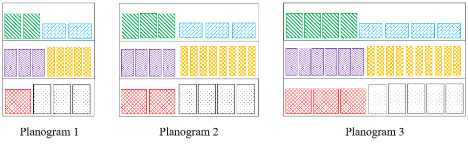
Figure 1: Sequence of planograms for a category with item facings and locations on shelves

Next, planners select a planogram for each relevant category and use software to automatically generate store layout. In the final step, planograms are physically replicated on store shelves. Using space planning software, retailers save a substantial amount of time on these space planning operations which otherwise would be carried out manually. Although space planning software provides efficient tools for visualizing and preparing of store layout and planograms and day-to-day maintenance and reporting activities, they are limited in incorporating the effect of space on sales and neglect to fully take advantage of mathematical optimization in floor space decisions. Planners decide the assignment of planograms to categories according to their experience and by employing heuristics (based on criteria sometimes called “proportional-to-market share”, and “proportional-to-profit share”). However, these decisions can be far from optimal (Desmet & Renaudin, 1998). First of all, space elasticity, the ratio of change in sales to change in space, is not considered. Secondly, the predicted revenue associated with various planograms is not known and not used to determine the best combination of planograms in a store to maximize total revenue.

Therefore, in our work we created an integrated solution using advanced mathematical modeling techniques in order to maximize revenue of each store. Our approach for FSO includes two steps: (1) develop a statistical model to measure the space elasticity; and (2) formulate and solve an optimization problem for each store to determine the optimal assignment of planograms to maximize total revenue subject to certain business constraints. Our statistical model is able to predict revenue of a product category for a given planogram, and in turn, the mathematical optimization efficiently determines the best assignment of planograms to categories. In this paper, our focus is on the design and implementation of a solution approach based on tabu search to solve the optimization problem in step (2).

In the early work on space modeling, the emphasis was placed on establishing a relation between space and sales. Indeed, the positive impact of space allocation on sales has been documented by several studies (Curhan, 1972; Corstjens & Doyle, 1981; Bultez et al., 1989; Borin et al., 1994; Dreze et al., 1994; Desmet & Renaudin, 1998). In light of research on space modeling, we developed a statistical model to measure the effect of allocated space in a planogram on category sales focusing on the solution of the space management optimization problem specified in Step (2) mentioned above. We refer the reader to Hübner & Kuhn (2012), Eisend (2014), Kök et al. (2015) and Bianchi-Aguiar et al. (2018) for holistic reviews of approaches to modeling of space effects.

In the second step of FSO, we maximize store revenues by optimally assigning planograms in stores. Modern revenue management launched with the airline industry and it advanced with the applications in two other traditional industries: hotels and car rental companies (Chiang et al., 2007). The success in these traditional industries attracted others and revenue management has since been applied in industries like restaurants, cargo, cruise, subscription services, theme parks and retail. More recently, revenue management has been introduced to newer industries such as cloud computing, home delivery, rideshare and e-commerce (Klein et al., 2020). Books by Talluri & Van Ryzin (2006) and Phillips (2005) provide introduction to concepts and aspects of revenue management including pricing, capacity allocation, network management, overbooking and markdown management and review papers by Chiang et al. (2007) and Klein et al. (2020) provide comprehensive surveys on the developments in revenue management over the last 40 years.

In the revenue management literature, FSO is considered as an application in the retail industry. Early applications of revenue management in retail started with seasonal items which are analogous to perishability of airline seat inventory. The value of the seasonal items diminish significantly after the selling season. Therefore, Coulter (2001) proposed the maximization of revenue by applying optimal discount pricing to seasonal items. In another study, Aviv & Pazgal (2005) investigated the dynamic pricing for fashion-like goods for a seasonal retailer. In their second work Aviv & Pazgal (2008), they extended their work to optimal pricing of seasonal goods in the presence of strategic customers. Practitioners Hawtin (2003) and Lippman (2003) provided overall guidelines on the implementation of revenue management systems in grocery retail outlets. They mainly focused on pricing strategy and discussed potential benefits and challenges in systems integration. In the recent years, revenue management for online retailers has been studied. Agatz et al. (2013) identified differentiation in price and delivery options as a key for revenue maximization. Belavina et al. (2017) analyzed the effect of subscription and per-order delivery revenue models on sales and environment for online grocery retailers.

As mentioned earlier, Kimes & Renaghan (2011) emphasized that space is the third strategic lever in revenue management, along with the price and time levers. They pointed out that space management is less studied in the literature, but is equally important as management of price and time. The aforementioned literature for retail revenue management mainly focuses on “price” and “time” levers and only includes “space” implicitly in some of the studies, i.e., none of the research works explicitly studied the effects of space allocation in optimizing revenues. Even though retailers manage time and price well, the performance will be sub-optimal in the context of revenue management if they do not manage their space well (Kimes & Renaghan, 2011). In our problem, all the levers are taken into account in the space-effect and optimization model where we explicitly optimize space by maximizing revenue per linear meter of a grocery store space for the implementation time period. FSO is an essential and integral component of any revenue management system that will enable retailers to achieve their revenue potential.

In sum, the floor space optimization problem considered here involves the optimal allocation of the available planograms in a store to maximize total predicted revenue. The problem is subject to constraints due to planogram sequencing, store layout, furniture and fixture characteristics. The first constraint requires that, for each existing planogram in a store, a replacement planogram should be chosen from its planogram sequence. This constraint ensures that every product category currently in the store is reassigned a planogram after the optimization. Space planners group the planograms with respect to furniture and fixture requirements and location in the store. These groups are called planogram worlds (PWs). The second constraint requires that the sum of lengths of planograms in each PW is bounded by lower and upper total length limits. Finally, the third constraint arises from the fact that a store can accommodate space expansion up to a certain level and requires space above some threshold. Therefore, this constraint imposes lower and upper limits on the total length of all planograms in the store (Additional background on the connection of FSO to other developments is given in the Appendix).

Intuitively, the FSO problem seems similar to the maximization version of the well-known knapsack problem (KP), as well as its variants such as multiple knapsack problems, or multiple choice knapsack problems, since we precalculate the expected revenues of planograms. If we view a planogram as an item, and a planogram world as a knapsack or bin, the FSO problem clearly contains the resource constraints (like the length limits) which are similar to knapsack constraints. For a comprehensive review on KP and its variants, we refer readers to Hiremath (2008). However, the additional global store length constraint of our FSO problem adds more complexities to the already complicated KP.

This paper develops a tabu search metaheuristic algorithm that exploits the specific neighborhood structures of the FSO problem. The next section defines the mathematical formulation of the FSO problem, and then provides a relevant literature review. In Section 3, we describe the tabu search algorithm specifically. The computational results are included in Section 4. Finally, we summarize our findings in Section 5.

2 Mathematical Formulation for FSO

The space model predicts revenue for a given space and other predictor variables of a product category in a planogram. Thus, we can define the predicted revenue of product category $i$ when assigned planogram $j$, $R_{ij}$ as

$$R_{ij}=h(s_{ij},{\mathbf{u}}_{ij}),$$

where $h(\cdot)$ represents the statistical model, $s_{ij}$ is the space assigned to category $i$ with planogram $j$, and $\mathbf{u}_{ij}$ is the vector of values for other predictor variables. Note that for the purposes of this study, the $R_{ij}$ values are precomputed and therefore assumed to be constants. The FSO problem can then be formulated as a mixed integer programming problem as follows.

Index:

• $I$: set of product categories

• $J$: set of planograms

• $K$: set of planogram worlds

• $J_{i}$: set of planograms that can be assigned to category $i$ where $\bigcap_{i\in I}J_{i}=\emptyset$

• $I_{k}$: set of categories belonging to PW $k$

• $J_{k}$: set of planograms belonging to PW $k$ where $J_{k}=\bigcup_{i\in I_{k}}J_{i}$

Constants:

• $R_{ij}$ : the revenue of category $i$ if assigned to planogram $j\in J_{i}$

• $L_{ij}$: the length (shelf space) for category $i$ if assigned to planogram $j\in J_{i}$

• $LL_{k}$: the lower bound of the total length for PW $k$

• $UL_{k}$: the upper bound of the total length for PW $k$

• $LS$: the lower bound on sum of all planogram lengths in the entire store

• $US$: the upper bound on sum of all planogram lengths in the entire store

Decision Variables: $x_{ij}$: the binary variable with value 1 if category $i$ is assigned to planogram $j$, and 0 otherwise.

Model:

Maximize $$\sum_{i\in I}\sum_{j\in J_{i}}R_{ij}x_{ij}$$ (1)

subject to $$\sum_{j\in J_{i}}x_{i,j}=1, \forall i\in I,$$ (2)

$$\sum_{i\in I_{k}}\sum_{j\in J_{i}}L_{ij}x_{ij}\geq LL_{k}, \forall k\in K,$$ (3)

$$\sum_{i\in I_{k}}\sum_{j\in J_{i}}L_{ij}x_{ij}\leq UL_{k}, \forall k\in K,$$ (4)

$$\sum_{i\in I}\sum_{j\in J_{i}}L_{ij}x_{ij}\geq LS,$$ (5)

$$\sum_{i\in I}\sum_{j\in J_{i}}L_{ij}x_{ij}\leq US,$$ (6)

$$x_{ij}\in\{0,1\}, \forall i\in I,j\in{J_{i}}.$$ (7)

The objective function (1) maximizes the total store revenue which is the sum of revenues of all categories placed on planograms. The constraint (2) stipulates each category should be assigned to a planogram. The constraints (3) and (4) establish the lower and upper length limits for each PW, and constraints (5) and (6) enforce the lower and upper limits of total planogram length for the store. The constraint (7) defines the binary variable for $x_{ij}$. Without the presence of constraints (5) and (6), the problem would be equivalent to solving $|K|$ multiple-choice KPs.

It is well known that the KP is NP-hard (Karp, 1972). The literature on KP and its variants is rich. Exact methods have focused on employing branch and bound and dynamic programming approaches (Martello & Toth, 1985, 1997, 2003; Martello et al., 1999; Pisinger, 1995, 1997, 1999a, 1999b). A variety of heuristics and metaheuristics have been designed for solving practical problems quickly, including those based on genetic algorithm (Chu & Beasley, 1997; Raidl, 1998), tabu search Glover & Kochenberger (1996); Lokketangen & Glover (1998), ant colony algorithms (Shi, 2006), simulated annealing (Liu et al., 2006), global harmony search (Zou et al., 2011), etc. In addition to the papers that have proposed algorithms, Pisinger (2005) conducted an interesting study on how to design test problems that appeared to be hard for several exact methods. Since FSO embeds a multiple choice KP-like NP hard subproblem, it is natural to develop a metaheuristic-based approach such as the tabu search algorithm for solving this practical problem.

3 The Tabu Search Algorithm for FSO

The tabu search (TS) algorithm is a well known metaheuristic for solving a large number of both theoretical and practical optimization problems. It employs adaptive memory to overcome the limitation of conventional search methods such as hill-climbing, which terminate (and hence become “trapped”) in a locally optimal solution within the current neighborhood. The common mechanisms TS employs include short term memory, long term memory, aspiration rule, intensification and diversification strategies. For a more comprehensive compendium of TS and its advanced strategies, we refer readers to Glover & Laguna (1997).

Our TS algorithm for FSO (denoted as TSFSO) starts from an initial solution and evaluates the objective function by calculating the revenues from planogram assignments and penalties from all length violations. Our method employs multiple simple neighborhood structures, and determines the moves based on these neighborhoods at each iteration through a scenario based control mechanism (controller). To improve the efficiency of the TS and reduce the effort spent on examining inferior solutions, we devise a learning-based candidate list strategy which benefits from the statistics collected from the search history. These components are elaborated in the next few subsections.

3.1 Initial Solution and Objective Function Evaluation

Our initial solution is constructed based on the following three simple rules:

1. Least length rule: each category is assigned to the planogram in which it occupies the least length.

   This rule ensures that violations of all upper limit length constraints will be minimized, but violations of the lower limit length constraints may occur.

2. Highest revenue rule: each category is assigned to the planogram where it will yield the highest revenue.

   This rule will produce a solution that achieves an upper bound on the revenue that can be obtained by an optimal FSO solution. However, violations to length constraints may occur coming from both upper and lower limits of the length constraints.

3. Balanced rule: each category is assigned to the planogram that yields the maximal revenue per length unit.

   This rule will generate a more balanced solution by considering both revenue and length requirements, though it may still cause violations of length constraints.

Let $G_{k}(x)$ denote the total length occupied by the current assignment $x$, that is $G_{k}(x)=\sum_{i\in I_{k}}\sum_{j\in J_{i}}L_{ij}x_{ij}$. Then we combine the revenue and violation into a single objective function in the TSFSO as follows:

$$f(x)= \sum_{i\in I}\sum_{j\in J_{i}}R_{ij}x_{ij}$$

$$-P\left(\sum_{k\in K}\left(\max(0,G_{k}(x)-UL_{k})+\max(0,LL_{k}-G_{k}(x))\right)\right.$$

$$\left.+\max(0,\sum_{k\in K}G_{k}(x)-US)+\max(0,LS-\sum_{k\in K}G_{k}(x))\right)$$

In the above objective, $P$ is a large positive number. When the assignment $x_{ij}$ is changed at each iteration, the value of $f(x)$ is recalculated accordingly. Upon termination, the $x_{ij}$ that produced the maximum value $f(x)$ is considered as the best solution. If the violation term associated with a solution is zero, then the solution is feasible.

3.2 Neighborhood Moves

The core decision of the FSO is to assign a planogram for each category to its corresponding PW. The neighborhood move is performed by assigning different planograms to categories iteratively. We design the five basic neighborhood moves as follows:

Level 1 Move: Select a category and move it from its current planogram to another planogram. In PW $k_{1}$, let $i_{1}$ be the category under consideration, let $j_{1}$ ($j_{1}\in J_{i_{1}}$) be the planogram that $i_{1}$ is currently assigned to, and $j_{2}$ is the new planogram ($j_{2}\neq j_{1}$, $j_{2}\in J_{i_{1}}$). Then the Level 1 Move changes the assignment $x_{i_{1}j_{1}}=1,x_{i_{1}j_{2}}=0$ to $x_{i_{1}j_{1}}=0,x_{i_{1}j_{2}}=1$. Such a move results in the following changes in objective function evaluation:

$$\Delta f(x)= R_{i_{1}j_{2}}-R_{i_{1}j_{1}}-P(\max(0,G_{k_{1}}(x)+L_{i_{1}j_{2}}-L_{i_{1}j_{1}}-UL_{k_{1}})$$

$$+\max(0,LL_{k_{1}}-G_{k_{1}}(x)-L_{i_{1}j_{2}}+L_{i_{1}j_{1}})+\max(0,\sum_{k\in K}G_{k}(x)$$

$$+L_{i_{1}j_{2}}-L_{i_{1}j_{1}}-US)+\max(0,LS-\sum_{k\in K}G_{k}(x)-L_{i_{1}j_{2}}+L_{i_{1}j_{1}}))$$

An example of a Level 1 Move is visually illustrated in Figure 2.

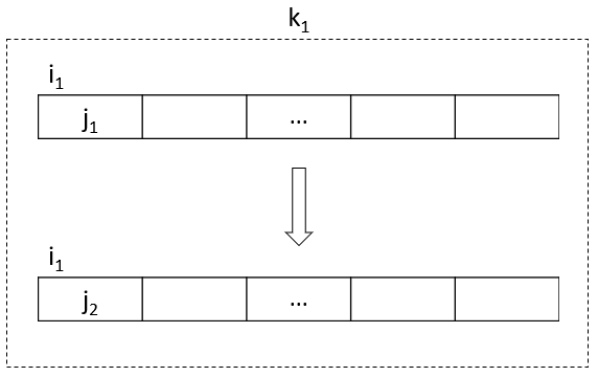
Figure 2: An Example of Level 1 Move

Once a Level 1 Move is performed, i.e., the category $i_{1}$ (in PW $k_{1}$) is moved from planogram $j_{1}$ to $j_{2}$, a tabu restriction is applied to prevent $i_{1}$ from being moved back to $j_{1}$ within a specific number of iterations. The duration (in iterations) of such a restriction is called the $tabu$ $tenure$ of the move, and is customarily selected randomly between a lower and upper bound. After a Level 1 Move (moving $i_{1}$ from $j_{1}$ to $j_{2}$), the reversed move (changing $x_{i_{1}j_{1}}=0$ to $x_{i_{1}j_{1}}=1$ is made $tabu$ for all iterations starting from the current iteration, $currIter$, through a last iteration $T(i,j)$ for $i=i_{1}$ and $j=j_{1}$ by the assignment:

$$T(i_{1},j_{1})=currIter+random(TL1,TH1)$$

where the value $random(TL1,TH1)$ identifies the tabu tenure based on the lower and upper bounds, $TL1$ and $TH1$. The value $T(i_{1},j_{1})$ may be called the (short-term) $tabu$ $memory$ for the move.

Level 2 Move: Select two categories from their current planograms (in PW $k_{1}$) to different planograms in the same PW. Let $i_{1}$, $i_{2}$ ($i_{1}\neq i_{2}$) be the two categories under consideration, let $j_{1}$, $j_{2}$ ($j_{1}\in J_{i_{1}},j_{2}\in J_{i_{2}}$) be the two currently assigned planograms for $i_{1}$ and $i_{2}$, and $j_{3}$ and $j_{4}$ be the new planograms ($j_{3}\neq j_{1}$, $j_{3}\in J_{i_{1}}$ , $j_{4}\neq j_{2}$, $j_{4}\in J_{i_{2}}$ ) for $i_{1}$ and $i_{2}$. Then the Level 2 Move changes the decision variable values from $x_{i_{1}j_{1}}=1,x_{i_{2}j_{2}}=1,x_{i_{1}j_{3}}=0,x_{i_{2}j_{4}}=0$ to $x_{i_{1}j_{1}}=0,x_{i_{2}j_{2}}=0,x_{i_{1}j_{3}}=1,x_{i_{2}j_{4}}=1$. Such a move results in the following changes in objective function evaluation:

$$\Delta f(x)= R_{i_{1}j_{3}}+R_{i_{2}j_{4}}-R_{i_{1}j_{1}}-R_{i_{2},j_{2}}-P(\max(0,G_{k_{1}}(x)+L_{i_{1}j_{3}}+L_{i_{2}j_{4}}$$

$$-L_{i_{1}j_{1}}-L_{i_{2}j_{2}}-UL_{k_{1}})+\max(0,LL_{k_{1}}-G_{k_{1}}(x)-L_{i_{1}j_{3}}-L_{i_{2}j_{4}}$$

$$+L_{i_{1}j_{1}}+L_{i_{2}j_{2}})+\max(0,\sum_{k\in K}G_{k}(x)+L_{i_{1}j_{3}}+L_{i_{2}j_{4}}-L_{i_{1}j_{1}}-L_{i_{2}j_{2}}$$

$$-US)+\max(0,LS-\sum_{k\in K}G_{k}(x)-L_{i_{1}j_{3}}-L_{i_{2}j_{4}}+L_{i_{1}j_{1}}+L_{i_{2}j_{2}}))$$

Figure 3 shows an example of a Level 2 Move.

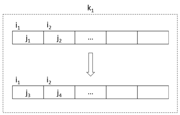
Figure 3: An Example of Level 2 Move

The tabu memory for a Level 2 Move (that moves category $i_{1}$ from planogram $j_{1}$ to $j_{3}$, and category $i_{2}$ from planogram $j_{2}$ to $j_{4}$) is to enforce $x_{i_{1}j_{1}}=0$ for all iterations less than or equal to $T(i_{1},j_{1})$ and $x_{i_{2}j_{2}}=0$ for all iterations less than or equal to $T(i_{2},j_{2})$. After such a Level 2 Move, the tabu memory is updated as:

$$T(i_{1},j_{1}) =currIter+random(TL2,TH2)$$

$$T(i_{2},j_{2}) =currIter+random(TL2,TH2)$$

Level 3 Move: Reassign three categories from their current planograms (in PW $k_{1}$) to different planograms in the same PW. Let $i_{1}$, $i_{2}$ and $i_{3}$ ($i_{1}\neq i_{2}$, $i_{2}\neq i_{3}$, $i_{3}\neq i_{1}$ be the three categories under consideration, let $j_{1}$, $j_{2}$ and $j_{3}$ ($j_{1}\in J_{i_{1}}$, $j_{2}\in J_{i_{2}}$, $j_{3}\in J_{i_{3}}$) be the three currently assigned planograms for $i_{1}$, $i_{2}$ and $i_{3}$, $j_{4}$, $j_{5}$ and $j_{6}$ be the new planograms ($j_{4}\neq j_{1}$, $j_{5}\neq j_{2}$, $j_{6}\neq j_{3}$, $j_{4}\in J_{i_{1}}$, $j_{5}\in J_{i_{2}}$ , $j_{6}\in J_{i_{3}}$) for these categories. Then the Level 3 Move changes the decision variable values from $x_{i_{1}j_{1}}=1$, $x_{i_{2}j_{2}}=1$, $x_{i_{3}j_{3}}=1$, $x_{i_{1}j_{4}}=0$, $x_{i_{2}j_{5}}=0$, $x_{i_{3}j_{6}}=0$ to $x_{i_{1}j_{1}}=0$, $x_{i_{2}j_{2}}=0$, $x_{i_{3}j_{3}}=0$, $x_{i_{1}j_{4}}=1$, $x_{i_{2}j_{5}}=1$, $x_{i_{3}j_{6}}=1$. Such a move results in the following changes in the objective function evaluation:

$$\Delta f(x)= R_{i_{1}j_{4}}+R_{i_{2}j_{5}}+R_{i_{3}j_{6}}-R_{i_{1}j_{1}}-R_{i_{2}j_{2}}-R_{i_{3}j_{3}}-P(\max(0,G_{k_{1}}(x)$$

$$+L_{i_{1}j_{4}}+L_{i_{2}j_{5}}+L_{i_{3}j_{6}}-L_{i_{1}j_{1}}-L_{i_{2}j_{2}}-L_{i_{3}j_{3}}-UL_{k_{1}})$$

$$+\max(0,LL_{k_{1}}-G_{k_{1}}(x)-L_{i_{1}j_{4}}-L_{i_{2}j_{5}}-L_{i_{3}j_{6}}+L_{i_{1}j_{1}}+L_{i_{2}j_{2}}$$

$$+L_{i_{3}j_{3}})+\max(0,\sum_{k\in K}G_{k}(x)+L_{i_{1}j_{4}}+L_{i_{2}j_{5}}+L_{i_{3}j_{6}}-L_{i_{1}j_{1}}-L_{i_{2}j_{2}}$$

$$-L_{i_{3}j_{3}}-US)+\max(0,LS-\sum_{k\in K}G_{k}(x)-L_{i_{1}j_{4}}-L_{i_{2}j_{5}}-L_{i_{3}j_{6}}$$

$$+L_{i_{1}j_{1}}+L_{i_{2}j_{2}}+L_{i_{3}j_{3}}))$$

Figure 4 displays an example of a Level 3 Move.

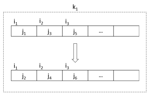
Figure 4: An Example of Level 3 Move

Similarly, after a Level 3 Move (that moves the category $i_{1}$ from planogram $j_{1}$ to $j_{4}$, and category $i_{2}$ from planogram $j_{2}$ to $j_{5}$, and category $j_{3}$ from planogram $j_{3}$ to $j_{6}$) , the tabu memory is updated by setting:

$$T(i_{1},j_{1}) =currIter+random(TL3,TH3)$$

$$T(i_{2},j_{2}) =currIter+random(TL3,TH3)$$

$$T(i_{3},j_{3}) =currIter+random(TL3,TH3)$$

Level 4 Move: Construct a composite move that performs the two Level 1 Moves simultaneously for two PWs. Let $i_{1}$ (in PW $k_{1}$) and $i_{2}$ (in PW $k_{2}$) be the two categories under consideration, let $j_{1}$ ($j_{1}\in J_{i_{1}}$) and $j_{2}$ ($j_{2}\in J_{i_{2}}$) be the planograms that hold $i_{1}$ and $i_{2}$, respectively. Finally, let $j_{3}$ and $j_{4}$ be the new planograms for $i_{1}$ and $i_{2}$ ($j_{3}\neq j_{1}$, $j_{3}\in J_{i_{1}}$, $j_{4}\neq j_{2}$, $j_{4}\in J_{i_{2}}$) for $i_{1}$ and $i_{2}$. Then the Level 4 Move changes the decision variable values from $x_{i_{1}j_{1}}=1$, $x_{i_{1}j_{3}}=0$, $x_{i_{2}j_{2}}=1$, $x_{i_{2}j_{4}}=0$ to $x_{i_{1}j_{1}}=0$, $x_{i_{1}j_{3}}=1$, $x_{i_{2}j_{2}}=0$, $x_{i_{2}j_{4}}=1$. Such a move results in the following changes in the objective function evaluation:

$$\Delta f(x)= R_{i_{1}j_{3}}-R_{i_{1}j_{1}}+R_{i_{2}j_{4}}-R_{i_{2}j_{2}}-P(\max(0,G_{k_{1}}(x)+L_{i_{1}j_{3}}$$

$$-L_{i_{1}j_{1}}-UL_{k_{1}})+\max(0,G_{k_{2}}(x)+L_{i_{2}j_{4}}-L_{i_{2}j_{2}}-UL_{k_{2}})$$

$$+\max(0,LL_{k_{1}}-G_{k_{1}}(x)-L_{i_{1}j_{3}}+L_{i_{1}j_{1}})+\max(0,LL_{k_{2}}$$

$$-G_{k_{2}}(x)-L_{i_{2}j_{4}}+L_{i_{2}j_{2}})+\max(0,\sum_{k\in K}G_{k}(x)+L_{i_{1}j_{3}}$$

$$-L_{i_{1}j_{1}}+L_{i_{2}j_{4}}-L_{i_{2}j_{2}}-US)+\max(0,LS-\sum_{k\in K}G_{k}(x)$$

$$-L_{i_{1}j_{3}}+L_{i_{1}j_{1}}-L_{i_{2}j_{2}}+L_{i_{2}j_{4}}))$$

Figure 5 depicts an example of a Level 4 Move where categories $i_{1}$ and $i_{2}$ are assigned to new planograms in the two PWs.

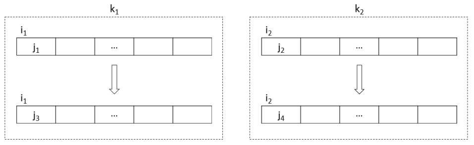
Figure 5: An Example of Level 4 Move

The tabu memory for a Level 4 Move (that moves category $i_{1}$ from planogram $j_{1}$ to $j_{3}$, and category $i_{2}$ from planogram $j_{2}$ to $j_{4}$) is updated as follows.

$$T(i_{1},j_{1}) =currIter+random(TL4,TH4)$$

$$T(i_{2},j_{2}) =currIter+random(TL4,TH4)$$

The difference between this and a Level 2 Move is that in the latter, the two categories $i_{1}$ and $i_{2}$ are located in the same PW, while in a Level 4 Move, they are located in the different PWs.

Level 5 Move: Like the Level 4 move, this move involves two PWs, in each PW two categories change their current planograms to the new planograms. Let $i_{1}$, $i_{2}$ (in PW $k_{1}$) and $i_{3}$, $i_{4}$ (in PW $k_{2}$) be the categories under consideration, and let $j_{1}$ ($j_{1}\in J_{i_{1}}$), $j_{2}$ ($j_{2}\in J_{i_{2}}$), $j_{3}$ ($j_{3}\in J_{i_{3}}$) and $j_{4}$ ($j_{4}\in J_{i_{4}}$) be the planograms that hold $i_{1},i_{2},i_{3}$ and $i_{4}$, respectively. Finally, let $j_{5}$ and $j_{6}$ be the new planograms for $i_{1}$ and $i_{2}$ ($j_{5}\neq j_{1}$, $j_{5}\in J_{i_{1}}$, $j_{6}\neq j_{2}$, $j_{6}\in J_{i_{2}}$), and let $j_{7}$ and $j_{8}$ be the new planograms for $i_{3}$ and $i_{4}$ ($j_{7}\neq j_{3}$, $j_{7}\in J_{i_{3}}$,$j_{8}\neq j_{4}$, $j_{8}\in J_{i_{4}}$ ). Then the Level 5 Move changes the decision variable values from $x_{i_{1}j_{1}}=1$, $x_{i_{1}j_{5}}=0$, $x_{i_{2}j_{2}}=1$, $x_{i_{2}j_{6}}=0$, $x_{i_{3}j_{3}}=1$, $x_{i_{3}j_{7}}=0$, $x_{i_{4}j_{4}}=1$, $x_{i_{4}j_{8}}=0$ to $x_{i_{1}j_{1}}=0$, $x_{i_{1}j_{5}}=1$, $x_{i_{2}j_{2}}=0$, $x_{i_{2}j_{6}}=1$, $x_{i_{3}j_{3}}=0$, $x_{i_{3}j_{7}}=1$, $x_{i_{4}j_{4}}=0$, $x_{i_{4}j_{8}}=1$. The changes in the objective function value are identified by :

$$\Delta f(x)= R_{i_{1}j_{5}}-R_{i_{1}j_{1}}+R_{i_{2}j_{6}}-R_{i_{2}j_{2}}+R_{i_{3}j_{7}}-R_{i_{3}j_{3}}+R_{i_{4}j_{8}}-R_{i_{4}j_{4}}$$

$$-P(\max(0,G_{k_{1}}(x)+L_{i_{1}j_{5}}-L_{i_{1}j_{1}}+L_{i_{2}j_{6}}-L_{i_{2}j_{2}}-UL_{k_{1}})$$

$$+\max(0,G_{k_{2}}(x)+L_{i_{3}j_{7}}-L_{i_{3}j_{3}}+L_{i_{4}j_{8}}-L_{i_{4}j_{4}}-UL_{k_{2}})$$

$$+\max(0,LL_{k_{1}}-G_{k_{1}}(x)-L_{i_{1}j_{5}}+L_{i_{1}j_{1}}-L_{i_{2}j_{6}}+L_{i_{2}j_{2}})$$

$$+\max(0,LL_{k_{2}}-G_{k_{2}}(x)-L_{i_{3}j_{7}}+L_{i_{3}j_{3}}-L_{i_{4}j_{8}}+L_{i_{4}j_{4}})$$

$$+\max(0,\sum_{k\in K}G_{k}(x)+L_{i_{1}j_{5}}-L_{i_{1}j_{1}}+L_{i_{2}j_{6}}-L_{i_{2}j_{2}}+L_{i_{3}j_{7}}$$

$$-L_{i_{3}j_{3}}+L_{i_{4}j_{8}}-L_{i_{4}j_{4}}-US)+\max(0,LS-\sum_{k\in K}G_{k}(x)$$

$$-L_{i_{1}j_{5}}+L_{i_{1}j_{1}}-L_{i_{2}j_{6}}+L_{i_{2}j_{2}}-L_{i_{3}j_{7}}-L_{i_{3}j_{3}}$$

$$-L_{i_{4}j_{8}}-L_{i_{4}j_{4}}))$$

Figure 6 exhibits an example of a Level 5 Move where categories $(i_{1},i_{2})$ and $(i_{3},i_{4})$ are assigned to new planograms in the two PWs.

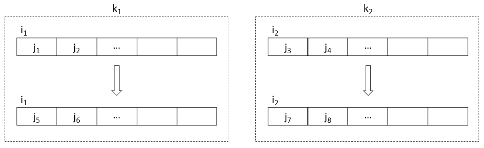
Figure 6: An Example of Level 5 Move

Similarly, the tabu memory for a Level 5 Move (that moves category $i_{1}$ from planogram $j_{1}$ to $j_{5}$, category $i_{2}$ from planogram $j_{2}$ to $j_{6}$, category $i_{3}$ from planogram $j_{3}$ to $j_{7}$, and category $i_{4}$ from planogram $j_{4}$ to $j_{8}$) is updated as:

$$T(i_{1},j_{1}) =currIter+random(TL5,TH5)$$

$$T(i_{2},j_{2}) =currIter+random(TL5,TH5)$$

$$T(i_{3},j_{3}) =currIter+random(TL5,TH5)$$

$$T(i_{4},j_{4}) =currIter+random(TL5,TH5)$$

Note that in TSFSO, once a type of neighborhood move is determined at each iteration, all legal moves from its respective neighborhood space are evaluated, and the move with the best evaluation subject to the corresponding tabu restrictions. If a better solution than the best solution found so far is detected, an $aspiration$ $rule$ permits the move to be performed regardless of the tabu memory restrictions. Other types of aspiration rules are also sometimes used, but the preceding rule is most often favored.

The type of move selected in TSFSO is determined by a scenario based control mechanism described next.

3.3 The Scenario-based Controller

Our use of multiple neighborhood moves, where each neighborhood provides a special structure for moving from one solution to another, is a type of strategy that is a critical element in meta-heuristics such as variable neighborhood search (VNS) (see Mladenović & Hansen, 1997). However, multiple neighborhoods strategies had already been successfully implemented in TS applications before the first VNS paper was published (see Glover et al., 1984; Xu et al., 1996; Xu & Kelly, 1996). In contrast to the VNS mechanism that allows the search to iterate over different neighborhoods, in such TS applications, a special control mechanism is designed to determine when to apply a specific neighborhood most efficiently and effectively. An example of this relevant to our current algorithm also appears in Xu et al. (1998).

In our five level neighborhoods, the lower level neighborhood moves are more effective for intensification to improve the current solution in regions around local optima, while the higher level neighborhood moves cause greater structural changes that move farther from a current solution and induce diversification. On the other hand, the number of move alternatives associated with the lower level neighborhoods is smaller than the number of alternatives associated with the higher level neighborhoods, and so the evaluation of the former is faster than that of the latter. Based on these observations, we design the following rules for the scenario-based controller by considering the balance between intensification and diversification, together with the trade-offs for efficiency. In the rules described below, a lower numbered rule can be overwritten by a higher numbered rule if, as indicated, this is valid for a specific scenario:

Rule 1:

During the first stage of the search ($T_{1}$ iterations), the Level 2 neighborhood is used to quickly improve the solution.

Rule 2:

During the second stage of the search ($T_{2}$ iterations), the lower level neighborhood moves are used probabilistically based on the probabilities as follows: $p_{1}$ for Level 1 neighborhood move, $p_{2}$ for Level 2 neighborhood move, and $p_{3}$ for Level 3 neighborhood move.

Rule 3:

During second stage of the search, whenever a new best ever solution is found, we “downgrade” neighborhood move type for the next iteration to reduce the current neighborhood move by one level. (This forces the search to focus more fully on intensification in an attempt to find an even better solution than the current new best solution.)

Rule 4:

At any iteration, if the current best solution could not be improved after a certain number of iterations denoted by $T_{3}$ (which often signals a search deadlock that requires a diversification strategy to break the impasse), a high level neighborhood (Level 4 or 5) move is required. The selection of the neighborhood is based on the probabilities $p_{4}$ for a Level 4 neighborhood and $p_{5}$ for a Level 5 neighborhood.

Rule 5:

If level 4 or 5 is selected per Rule 4, then this level cannot be performed for more than $T_{4}$ consecutive iterations. Once $T_{4}$ consecutive iterations of Level 4 or 5 moves are used, then the search must be switched back to a lower level neighborhood (Level 1,2,or 3, the exact type to use is determined probabilistically by Rule 2.) for at least $T_{5}$ iterations. (Rule 5 prevents the search from focusing too long on diversification strategies when these strategies are not successful in improving the best solution. This allows the search to strategically oscillate between the intensification and diversification strategies.)

Rule 6:

The search terminates either when the maximum number of iterations is reached ($T_{0}=T_{1}+T_{2}$), or when the search cannot improve the current best feasible solution for $T_{6}$ iterations.

In Rules 2 and 4, a randomization based probabilistic selection method is used for iterating between the different types of neighborhoods. This allows the search to overcome the strong local optimality tendency produced by adhering to a single neighborhood and amplifies the diversification effect. The scenario-triggered rules (which are invoked when (1) a quick improvement is required during early search; (2) a new best solution is found; (3) the search fails to find a new best solution for a certain time, etc.) are applied to enhance the ability to exploit the special neighborhood structures of various neighborhoods, while accounting for issues of effectiveness and efficiency.

3.4 The Learning-based Candidate List Strategy

To further improve the efficiency of TSFSO, we consider the fact that a good neighborhood move may contain attribute values similar to those of good neighborhood moves performed in the past. For this, we employ a $candidate$ $list$ to guide our choice of moves based on keeping track of attributes contained in good past moves.

We collect statistics from the moves performed at each of the first $T_{7}$ iterations in the search history and count the frequency of the PW/category combinations of the moves executed at each iteration. Let $U_{ki}$ be the number of times that PW $k$ and category $i$ are involved in the moves performed so far, where initially $U_{ki}$ is set to zero, and $U_{ki}$ is updated at each iteration as follows.

Table 1: Move Attributes Statistics Collection

Performed Move Type	Involved PW/Category	Update $U_{ki}$
Level 1	$(k,i)$	$U_{ki}=U_{ki}+1$
Level 2	$\begin{array}[]{l}(k,i_{1})\\ (k,i_{2})\end{array}$	$\begin{array}[]{l}U_{ki_{1}}=U_{ki_{1}}+1\\ U_{ki_{2}}=U_{ki_{2}}+1\end{array}$
Level 3	$\begin{array}[]{l}(k,i_{1})\\ (k,i_{2})\\ (k,i_{3})\end{array}$	$\begin{array}[]{l}U_{ki_{1}}=U_{ki_{1}}+1\\ U_{ki_{2}}=U_{ki_{2}}+1\\ U_{ki_{3}}=U_{ki_{3}}+1\end{array}$
Level 4	$\begin{array}[]{l}(k_{1},i_{1})\\ (k_{2},i_{2})\end{array}$	$\begin{array}[]{l}U_{k_{1}i_{1}}=U_{k_{1}i_{1}}+1\\ U_{k_{2}i_{2}}=U_{k_{2}i_{2}}+1\end{array}$
Level 5	$\begin{array}[]{l}(k_{1},i_{1})\\ (k_{1},i_{2})\\ (k_{2},i_{3})\\ (k_{2},i_{4})\end{array}$	$\begin{array}[]{l}U_{k_{1}i_{1}}=U_{k_{1}i_{1}}+1\\ U_{k_{1}i_{2}}=U_{k_{1}i_{2}}+1\\ U_{k_{2}i_{3}}=U_{k_{2}i_{3}}+1\\ U_{k_{2}i_{4}}=U_{k_{2}i_{4}}+1\end{array}$

After the statistics $U_{ki}$ are collected from the first $T_{7}$ iterations, we construct a candidate list at each iteration thereafter for each type of neighborhood move performed at that iteration. The updating of the $U_{ki}$ values is continued, however, until the end of the search. For categories $I_{k}$ of PW $k$, let $n_{k}$ be the number of categories in $I_{k}$ that are included in the moves performed so far ($n_{k}\leq|I_{k}|$), and let $\bar{U}_{k}=\{i^{\prime}_{1},i^{\prime}_{2},...,i^{\prime}_{n_{k}}\}$ be a sorted list of category indices such that $U_{ki^{\prime}_{1},}\geq U_{ki^{\prime}_{2}}\geq...\geq U_{ki^{\prime}_{n_{k}}}>0$.

We further introduce a list $\bar{U}_{k}(n_{k})$ containing the first $n_{k}$ category indices from $\bar{U}_{k}$ ($p\leq n_{k}$) (with $n_{k}$ identifying the highest $U_{ki}$ value category). The candidate list construction is described in Table 2.

Table 2: Candidate List Construction

Performed Move Type	Involved PW/Category	Candidate List
Level 1	$(k,i)$	$\begin{array}[]{l}\mbox{No candidate list; use the full neighborhood,}\\ \mbox{i.e., }i\mbox{ is selected from }I_{k}.\end{array}$
Level 2	$\begin{array}[]{l}(k,i_{1})\\ (k,i_{2})\end{array}$	$\begin{array}[]{l}\mbox{For PW }k,\mbox{if }|\bar{U}_{k}|>0,\mbox{then }i_{1},i_{2}\mbox{ are selected from the}\\ \mbox{category list }\bar{U}_{k}(n_{k}*r_{1});\\ \mbox{Otherwise,}i_{1},i_{2}\mbox{ are selected from }I_{k}.\end{array}$
Level 3	$\begin{array}[]{l}(k,i_{1})\\ (k,i_{2})\\ (k,i_{3})\end{array}$	$\begin{array}[]{l}\mbox{For PW }k,\mbox{if }|\bar{U}_{k}|>0,\mbox{then }i_{1},i_{2},i_{3}\mbox{ are selected from }\\ \mbox{the category list }\bar{U}_{k}(n_{k}*r_{1});\\ \mbox{Otherwise, }i_{1},i_{2},i_{3}\mbox{ are selected from }I_{k}.\end{array}$
Level 4	$\begin{array}[]{l}(k_{1},i_{1})\\ (k_{2},i_{2})\end{array}$	$\begin{array}[]{l}\mbox{For PW }k_{1},\mbox{if }|\bar{U}_{k_{1}}|>0,\mbox{then }i_{1}\mbox{ is selected}\\ \mbox{from the category list }\bar{U}_{k_{1}}(n_{k_{1}}*r_{2});\\ \mbox{Otherwise, }i_{1}\mbox{ is selected from }IA_{s_{1}};\\ \mbox{For PW }k_{2},\mbox{if }|\bar{U}_{k_{2}}|>0,\mbox{ then }i_{2}\mbox{ is selected from }\\ \mbox{the category list }\bar{U}_{k_{2}}(n_{k_{2}}*r_{2});\\ \mbox{Otherwise, }i_{2}\mbox{ is selected from }I_{k_{2}}.\end{array}$
Level 5	$\begin{array}[]{l}(k_{1},i_{1})\\ (k_{1},i_{2})\\ (k_{2},i_{3})\\ (k_{2},i_{4})\end{array}$	$\begin{array}[]{l}\mbox{For PW }k_{1},\mbox{if }|\bar{U}_{k_{1}}|>0,\mbox{then }i_{1},i_{2}\mbox{ are selected from }\\ \mbox{the category list }\bar{U}_{k_{1}}(n_{k_{1}}*r_{2});\\ \mbox{Otherwise, }i_{1},i_{2}\mbox{ are selected from }I_{k_{1}};\\ \mbox{For PW }k_{2},\mbox{if }|\bar{U}_{k_{2}}|>0,\mbox{then }i_{3},i_{4}\mbox{ are selected from }\\ \mbox{the category list }\bar{U}_{k_{2}}(n_{k_{2}}*r_{2});\\ \mbox{Otherwise, }i_{3},i_{4}\mbox{ are selected from }I_{k_{2}}\end{array}$

In TSFSO, the ratios $r_{1}$ and $r_{2}$ indicate the degree of reduction from the full neighborhoods. The smaller the values for $r_{1}$ and $r_{2}$, the more compressed is the neighborhood used for the respective candidate list.

4 Computational Results

TSFSO algorithm is implemented for the real floor space planning problem arising in a leading grocery chain in Europe. To investigate the effectiveness of TSFSO, we need to execute our TSFSO on a series of test problems. Since there are no known open benchmark problems available for FSO, we first design a method to generate a series of test problems. We utilize store space configuration data from our real world implementation, as well as ideas for designing hard test problem instances for relevant knapsack problems in literature. We describe the test problem generation method in the next subsection.

4.1 Test Problem Generation

We choose a common store in the grocery chain with 9 PWs and 194 planograms and use its actual PW/planogram configuration as a basis for our test problem generation. To protect confidential information such as planogram length and revenue data for the company, we generated associated length ($L_{ij}$) and revenue ($R_{ij}$) data using an approach which aims to create difficult test instances for knapsack problems based on existing research in literature. More specifically, we use a method to create the so-called weakly correlated spanner instances with span(2,10) described in Pisinger (2005) to generate a series of coordinated pairs of length and revenue data as follows. We first generated a basic spanner set $(l_{\kappa},r_{\kappa})$ for $\kappa\in\{1,2\}$ by setting $l_{\kappa}=random(1,10^{7})$, and $r_{\kappa}=random(l_{\kappa}-10^{6},l_{\kappa}+10^{6})$ for $\kappa\in\{1,2\}$. If the resulting $r_{\kappa}<1$, we regenerate $r_{\kappa}$ until it satisfies $r_{\kappa}\geq 1$. Then we normalize the spanner set by setting $l_{\kappa}=\lceil l_{\kappa}/5\rceil,r_{\kappa}=\lceil r_{\kappa}/5\rceil$ for $\kappa\in\{1,2\}$. Then each pair of length and revenue numbers $(L_{ij},R_{ij})$ is generated by repeatedly taking one pair ($l_{\kappa},r_{\kappa}$) from the spanner set, and multiplying it by a value randomly generated from $[1,10]$.

In particular, we initialize the counter $k=0$ and for each valid combination of $(i,j)$, we identify the spanner set index by $\kappa=k\textrm{ mod }2+1$, $\alpha=random(1,10)$. The length and revenue numbers are then calculated as $L_{i,j}=\alpha l_{k}$ and $R_{ij}=\alpha r_{k}$, followed by incrementing the counter $k$ by setting $k=k+1$. We repeat the process until all possible length and revenue values $(L_{ij},R_{ij})$ are generated for the required 194 planograms.

Unlike the method suggested in Pisinger (2005) where the length bounds are generated based on the generated lengths using different ratios across test instances (e.g., bounds are increased by a fixed percentage for each instance), however, we generated the lower and upper bounds for PWs and store levels for our test problems by multiplying fixed ratios (0.85 for lower bound and 1.15 for upper bound) with total (generated) lengths calculated based on the current planogram assignment. This approach may reduce the difficulty of the test problems but ensures the generated problems are feasible and bounds are consistent with the current store FSO planning practice as well. Nevertheless, the test problems we generated are still computationally more difficult than the real problem we encountered in practice, indicating that they are good problems to stress-test our TSFSO heuristic and to have some confidence that our heuristic can cover realistic problems we have yet to encounter.

We repeat the above process using different random seeds until we generate 100 test problems. To execute our TSFSO on these test problems, we use the parameter values described in the next subsection.

4.2 Parameter Setting

We set the values for the parameters based on a priori knowledge, as well as on the results from limited brute-force experiments. Applying a systematic parameter fine-tuning method based on statistical analysis and experiment design techniques may significantly improve the heuristic performance (see Xu $et$ $al.$ 1998b for an example).

First, the penalty $P$ for length violations (at both the PW level and store level) is set to $-20000$. In this application, the penalty function is implemented as a static value, heavily emphasizing feasibility over solution quality by strongly favoring feasible neighborhood moves, and hence focusing more intensification than diversification. We plan in a future work to design a dynamic, self-adaptive penalty parameter, to better explore the interplay between intensification and diversification.

Tabu tenure parameters are set as follows: we unify such parameters for various neighborhood move types by designating a single lower bound and a single upper bound. Such bounds are related to the respective neighborhood spaces so they can be resiliently applied to small, medium or large neighborhoods. Specifically, for a given PW $k$, we set the lower bound value $TL=TL1=TL1=TL3=TL4=TL5=\max\{4,|I_{k}|/2\}$, and the upper bound value $TH=TH1=TH1=TH3=TH4=TH5=TL+\min\{7,|I_{k}|/7\}$.

Several parameters govern the controller and the search progress. The entire search consists of 1200 iterations ($T_{0}=1200$), while the first stage of the search starts from iteration 1 to iteration $T_{1}=120$ and the second stage then invokes for the reset of $T_{2}=1080$ iterations. The parameter $T_{3}$, which triggers the condition for using high level neighborhood moves, is set to 20 iterations. The high level neighborhood moves can be performed no more than 2 consecutive iterations ($T_{4}=2$) and the next 10 iterations ($T_{5}=10$) will be dedicated to low level neighborhood moves after 2 consecutive iterations for high level neighborhood moves. The TSFSO terminates either when the iteration counter reaches $T_{0}=1200$, or when the current (feasible) best solution cannot be improved within the most recent $T_{6}=0.8*T_{0}$ iterations.

The probabilities used for selecting the different types of neighborhood moves are: $p_{1}=0.2,p_{2}=0.5,p_{3}=0.3,p_{4}=0.6,p_{5}=0.4$. Note that $p_{1}+p_{2}+p_{3}=1.0$ and $p_{4}+p_{5}=1.0$.

Lastly, the candidate list strategy collects statistics from attributes of moves performed during the first 100 ($T_{7}=100$) iterations. Consequently, the candidate list strategy is initiated at the $101^{st}$ iteration. The two ratios used to reduce the neighborhood spaces, are set to $r_{1}=0.5$, $r_{2}=0.8$, respectively.

4.3 Computational Experiments and Results Analysis

The TSFSO is implemented using the Python language and is executed on a Linux machine on cloud. The CPU model of the machine is Intel^® Xeon^® CPU E5-2686 v4 @ 2.30GHz. To compare the effectiveness of TSFSO, we first use Gurobi, one of the leading commercial solver packages for Mixed Integer Programming, to solve the 100 tests problems to optimality using the same computational environment. We limit the computation time to 200 seconds for each problem. Gurobi either finds an optimal solution before reaching the time limit or terminates with a best solution obtained at the time limit, which we designate it as the $defacto$ optimal solution, instead of classifying it as an optimal solution.

To evaluate the different time effect of TSFSO, we set the maximum number of iterations ($T_{0}$ in the four test runs of TSFSO to be 300, 600, 900, and 1,200. The associated test runs are accordingly denoted TSFSO-300, TSFSO-600, TSFSO-900, TSFSO-1200. All other parameters remain the same as previously described with the following features implemented:

• used the balanced rule as the initial solution rule;

• used all 5 level moves coordinated by the scenario-based controller; and

• used candidate list.

In summarizing the results from across the 100 problems, we report the number of problems for which we obtain an optimal or $defacto$ optimal solution (as OPTNUM), the average percentage of the optimality gap across all 100 problems (as AVGGAP), maximum percentage of the optimality gap (as MAXGAP), and the total CPU time in seconds (as CPUTM) in Table 3.

Table 3: Computational Results on 100 Test Problems

RUN	OPTNUM	AVGGAP(%)	MAXGAP(%)	CPUTM
TSFSO-300	35	0.23	0.96	59
TSFSO-600	68	0.08	0.52	154
TSFSO-900	83	0.04	0.52	217
TSFSO-1200	100	0.00	0.00	312
Gurobi	100	0.00	0.00	12,345

Table 3 clearly demonstrates with the reported reasonable computational times that our TSFSO algorithm can overcome the computational intractability of the test problems and obtain exceedingly high quality solutions using just a fraction of the time required by the Gurobi solver. Although for iteration limits below 1,200, not all optimal solutions were attained, the maximum percentage gap is quite small at less than $1\%$, and these solutions were obtained by our TSFSO at significantly less computational time versus Gurobi. This further confirms that TSFSO can be used as an effective practical optimization method for solving floor space optimization problems without relying on commercial proprietary solvers such as Gurobi. It should be noted that our TSFSO was implemented in Python, which is generally considered slower in computational speed as compared to the C language that Gurobi was implemented on.

Next, we run experiments on our TSFSO to determine the effects of the three different initial solution rules described in Section 3.1. We denote the TSFSO using the least length rule, the highest revenue rule, and the balanced rule as TSFSO-LL, TSFSO-HR, and TSFSO-1200, respectively. All such TSFSO variants use 1200 iterations which offers sufficient time to improve the solution quality using tabu search.

Table 4: Comparison of Initial Solution Rules

RUN	OPTNUM	AVGGAP(%)	MAXGAP(%)	CPUTM
TSFSO-LL	39	0.22	0.91	310
TSFSO-HR	26	0.33	1.40	314
TSFSO-1200	100	0.00	0.00	312

The results in Table 4 clearly shows that TSFSO with different initial solution rules can find very high quality solutions for FSO. Compared to the optimal (or $defacto$ optimal) solutions, the TSFSO using the balanced rules for generating initial solutions yields all optimal solutions for all cases, and the one using the least length rule for initial solutions obtains 39 optimal solutions out of 100 cases. The TSFSO using the highest revenue rule based initial solutions lags behind by obtaining 26 optimal solutions; however, the worst solution is only $1.4\%$ away from optimality (on average it is 0.33%), indicating it can produce reliable high quality solutions for practical applications.

By carefully monitoring and comparing the search progress, we cannot conclude that the computation time is significantly sensitive to the choice of initial solution method. No matter which initial solution method is adapter, the TSFSO beats Gurobi by an obvious edge in computation time.

We use TSFSO-1200 as a basis for examining the effects of using multiple neighborhoods in TSFSO by comparing to the tests from those using a single type of neighborhood for Level 1, Level 2, Level 3, Level 4 and Level 5 moves, denoting these tests by TSFSO-1, TSFSO-2, TSFSO-3, TSFSO-4 and TSFSO-5 in Table 5. We also design a new test, designated TSFSO-NC, that deactivates the learning-based candidate list in TSFSO-1200. In addition to the values OPTNUM, AVGGAP, MAXGAP and CPUTM reported in the previous table, we also show in the column INFNUM the number of cases in which the runs fail to find a feasible solution when the algorithm terminated.

Table 5: Comparison of Neighborhoods and Candidate List Strategy

RUN	OPTNUM	INFNUM	AVGGAP(%)∗	MAXGAP(%)∗	CPUTM
TSFSO-1200	100	0	0.00	0.00	312
TSFSO-1	0	46	3.25	19.20	4
TSFSO-2	0	100	N/A	N/A	109
TSFSO-3	0	100	N/A	N/A	743
TSFSO-4	0	25	1.81	19.40	99
TSFSO-5	0	100	N/A	N/A	8,272
TSFSO-NC	91	0	0.02	0.48	2,731

^∗ applies to feasible cases only

It is obvious in Table 5 that the TSFSO version that uses multiple neighborhoods performs better than the versions equipped with a single type of neighborhood. None of the single neighborhood versions can compete with TSFSO-1200 in terms of the number of optimal/feasible solution obtained. As shown, the Level 1 neighborhood move is the fastest but is able to obtain feasible solutions only for 54 cases. Moreover, it yields not a single optimal solution, and the average optimality gap of $3.25\%$. Level 4 neighborhood moves, which perform two Level 1 moves simultaneously, provide significant improvements in term of the feasible solutions obtained. The Level 2, 3 and 5 neighborhood moves, each of which changes more than one assignment for one or two PWs, can hardly find feasible solutions by solely relying on their own effort. This confirms that each type of move has its own unique merits and disadvantages for handling special problem structures. In combination, they complement each other to find superior solutions, as shown in our baseline TSFSO-1200 version.

Surprisingly, the high level Level 4 neighborhood moves perform slightly faster than the lower level Level 2 moves. We attribute this mainly to the fact that the Level 4 moves enable the algorithm to reach a feasible local optimal solution quickly in 75 cases. In each iteration, it may move to the first improving best solution without examining the whole neighborhood space. In contrast, the Level 2 move version struggles to achieve feasibility, so it consequently searches the entire neighborhood space at each iteration, and finally terminates without finding a feasible solution.

The findings from the comparisons between TSFSO-1200 and TSFSO-NC also confirm that the learning-based candidate list strategy can effectively improve efficiency using only $11.4\%$ of the computation time required by the version without learning-based candidate list strategy (312 seconds versus 2,731 seconds). It is also interesting to note that the full neighborhood search performed in TSFSO-NC does not always yield optimal solutions, though in the 9 cases it obtained solutions with exceedingly small optimality gaps.

Next, we examine the effects of tabu memory in TSFSO. We again use TSFSO-1200 as the base case and obtain varying cases to experiment as follows: (a) no tabu memory is applied; (b) all tabu tenures are set to 4; (c) all tabu tenures are set to 7; (d) $TL=TH=(\max\{4,|I_{k}|/2\}+min\{7,|I_{k}|/7\})/2$. The corresponding new tests are denoted TSFSO-a, TSFSO-b, TSFSO-c and TSFSO-d. Table 6 contains the results from these tests along with the baseline run TSFSO-1200.

Table 6: Comparison of Different Tabu Memories

RUN	OPTNUM	AVGGAP(%)	MAXGAP(%)	CPUTM
TSFSO-1200	100	0	0	312
TSFSO-a	0	0.87	2.5	458
TSFSO-b	16	0.39	1.5	377
TSFSO-c	32	0.25	1.05	339
TSFSO-d	47	0.0.21	1.93	324

As shown in Table 6, all tests obtain feasible solutions with marginal optimality gaps. This can be partially attributed to the efficiency of the multiple neighborhood search method designed for TSFSO. The contribution of the tabu memory to this outcome is quite noticeable. However, when the tabu memory is removed (TSFSO-a), the algorithm fails to obtain any optimal solutions in any of the 100 cases. Upon implementing various tabu memory methods (TSFSO-b, TSFSO-c, TSFSO-d), the number of optimal solutions improved and the optimality gaps diminished for non-optimal cases. This demonstrates the value of tabu memory for improving an already good multiple neighborhood procedure by providing the ability to escape from strong locally optimal solutions. The baseline version of our algorithm (TSFSO-1200) which determines the tabu tenure as indicated in Section 4.2 clearly outperforms the others.

In addition, based on the results shown in Table 6, tabu memory not only plays critical role in obtaining optimal or near optimal solutions, but also helpful in improving the efficiency with reduced computational time. This finding is consistent with our observation that those TSFSO variants without tabu memory or with simple implementation of tabu memory intend to use more complicated and time consuming neighborhood move types (i.e., type 3 or type 5 moves), since they may encounter search impasse more frequently. An appropriate design of tabu memory is one of the key factors for practical FSO applications that requires obtaining high quality solutions within reasonable amount of computing time.

Finally, we demonstrate an example of the search progression of TSFSO for a selected run from our practical implementation in Figure 7. In this figure, the top and bottom charts show the value of the objective function $f(x)$ as well as the sum of the length constraint violations of the move performed at each iteration. (A zero violation indicates a feasible solution). The horizontal axis represents the iteration number, and the values of the vertical axis ($f(x)$ and violations) are transformed and re-scaled artificially (without loss of trends) for better illustrative purposes. Note the maximum number of iterations $T_{0}$ is set to 350 in this run.

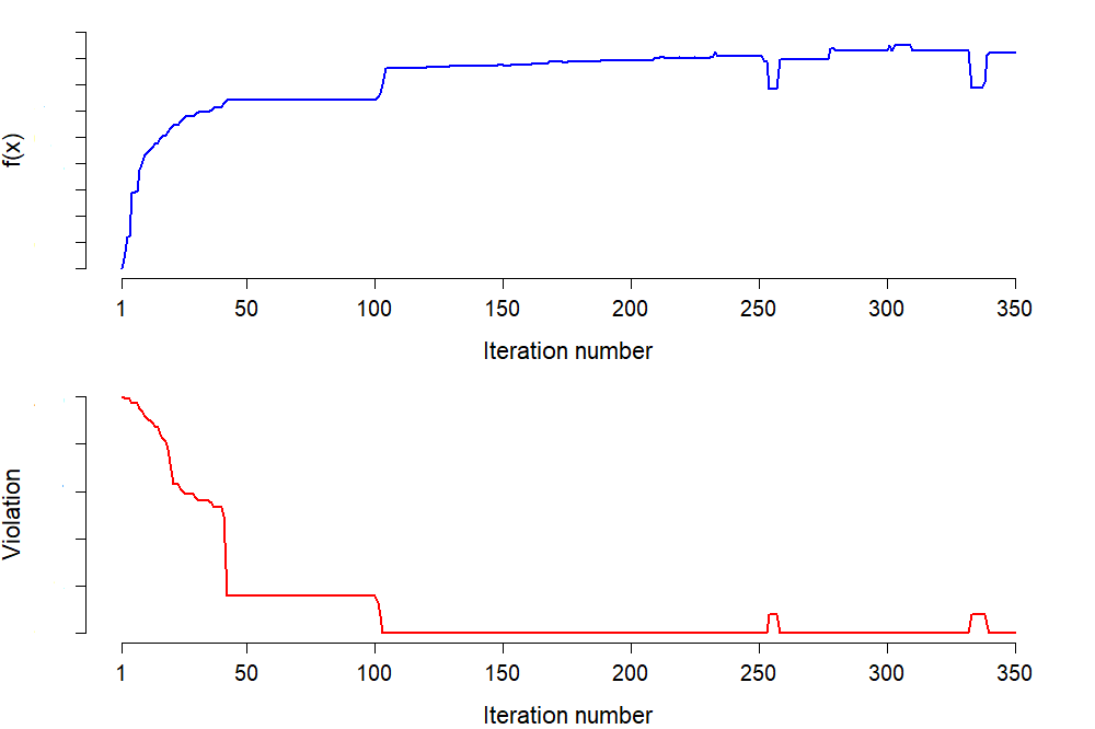
Figure 7: A Search Progress Example

Figure 7 demonstrates that the TSFSO can rapidly improve solution quality after starting from an initial solution with a large feasibility violation. With the help of the large penalty, the solution becomes feasible at $103^{rd}$ iteration, and continues to improve via the multiple neighborhood moves. A locally optimal solution is obtained at the $233^{rd}$ iteration. Then the search continues, escaping the local optimum with the assistance of tabu memory. The search falls into an infeasible region at the $254^{th}$ iteration, and moves back into a feasible region at the $258^{th}$ iteration. The algorithm finds two new best solutions at the $278^{th}$ and $301^{st}$ iterations, and then again enters an infeasible region between iterations $333$ and $340$. No new best solutions were found throughout the remainder of the search, which terminated at the $350^{th}$ iteration.

5 Conclusion

We studied the floor space optimization problem arising in retail store revenue management by providing a mathematical formulation, conducting a review of relevant research and proposing a new solution approach based on tabu search. Our tabu search algorithm contains several innovative components, including a scenario-based controller for combining the multiple neighborhoods, and a candidate list strategy that utilizes learning based on statistics collected from prior search history.

We applied our TSFSO on 100 test problems that combined the practical configuration from real world applications as well as results from computational studies in literature. We reported results demonstrating that our method is highly effective and efficient in handling the test problems. Analysis of the experiment results further confirms the value of our scenario-based controller and our learning-based candidate list strategy. The use of the TSFSO in a practical application to a grocery chain improved its predicted annual revenue by around 1%, which amounts to approximately 80 million Euros.

Future research work will continue in two directions: model improvement and algorithm improvement. First, we plan to enrich the space-effect and optimization models by considering planogram orientations, relative positions and layout. Mowrey et al. (2018, 2019) studied the impact of layout and orientation of racks in a store on customer’s navigation and exposure which provide guidance on how to allocate planograms in a store to maximize revenue. Because space is relatively fixed and scarce in a store, the inclusion of these additional aspects will improve the forecasting from the space-effect model and provide additional depth to the optimization model. Secondly, we will further improve the efficacy of TSFSO. Among the improvements envisioned, we plan to introduce a self-adaptive penalty function to replace the current reliance on a fixed penalty value that penalizes feasibility violations. We also plan to study other potential improvements such as the analysis of the patterns of moves that prove most effective in order to further improve the search efficiency, the investigation of more advanced mechanisms to control the interplay between intensification and diversification, and the exploration of path relinking strategies to construct and exploit search trajectories between good solutions.

References

- (1)
- Agatz et al. (2013) Agatz, N., Campbell, A. M., Fleischmann, M., Van Nunen, J. & Savelsbergh, M. (2013), ‘Revenue management opportunities for internet retailers’, Journal of Revenue and Pricing Management 12(2), 128–138.
- Aviv & Pazgal (2005) Aviv, Y. & Pazgal, A. (2005), ‘A partially observed markov decision process for dynamic pricing’, Management science 51(9), 1400–1416.
- Aviv & Pazgal (2008) Aviv, Y. & Pazgal, A. (2008), ‘Optimal pricing of seasonal products in the presence of forward-looking consumers’, Manufacturing & service operations management 10(3), 339–359.
- Belavina et al. (2017) Belavina, E., Girotra, K. & Kabra, A. (2017), ‘Online grocery retail: Revenue models and environmental impact’, Management Science 63(6), 1781–1799.
- Bianchi-Aguiar et al. (2018) Bianchi-Aguiar, T., Silva, E., Guimarães, L., Carravilla, M. A. & Oliveira, J. F. (2018), ‘Allocating products on shelves under merchandising rules: Multi-level product families with display directions’, Omega 76, 47–62.
- Borin et al. (1994) Borin, N., Farris, P. W. & Freeland, J. R. (1994), ‘A model for determining retail product category assortment and shelf space allocation’, Decision sciences 25(3), 359–384.
- Bultez et al. (1989) Bultez, A., Naert, P., Gijsbrechts, E. & Abeele, P. V. (1989), ‘Asymmetric cannibalism in retail assortments’, Journal of Retailing 65(2), 153.
- Chiang et al. (2007) Chiang, W.-C., Chen, J. C. & Xu, X. (2007), ‘An overview of research on revenue management: current issues and future research’, International journal of revenue management 1(1), 97–128.
- Chu & Beasley (1997) Chu, P. C. & Beasley, J. E. (1997), ‘A genetic algorithm for the generalised assignment problem’, Computers & Operations Research 24(1), 17–23.
- Corstjens & Doyle (1981) Corstjens, M. & Doyle, P. (1981), ‘A model for optimizing retail space allocations’, Management Science 27(7), 822–833.
- Coulter (2001) Coulter, K. S. (2001), ‘Decreasing price sensitivity involving physical product inventory: a yield management application’, Journal of Product & Brand Management .
- Curhan (1972) Curhan, R. C. (1972), ‘The relationship between shelf space and unit sales in supermarkets’, Journal of Marketing Research 9(4), 406–412.
- Desmet & Renaudin (1998) Desmet, P. & Renaudin, V. (1998), ‘Estimation of product category sales responsiveness to allocated shelf space’, International Journal of Research in Marketing 15(5), 443–457.
- Dreze et al. (1994) Dreze, X., Hoch, S. J. & Purk, M. E. (1994), ‘Shelf management and space elasticity’, Journal of retailing 70(4), 301–326.
- EHI Retail Institute (2014) EHI Retail Institute (2014), Retail data 2014: Structure, key figures and profiles of international retailing, White paper, EHI Retail Institute, Cologne.
- Eisend (2014) Eisend, M. (2014), ‘Shelf space elasticity: A meta-analysis’, Journal of Retailing 90(2), 168–181.
- Glover & Kochenberger (1996) Glover, F. & Kochenberger, G. A. (1996), Critical event tabu search for multidimensional knapsack problems, in I. H. Osman & J. P. Kelly, eds, ‘Meta-heuristics’, Springer, pp. 407–427.
- Glover & Laguna (1997) Glover, F. & Laguna, M. (1997), Tabu Search, Kluwer Academic Publishers, USA.
- Glover et al. (1984) Glover, F., McMillan, C. & Glover, R. (1984), ‘A heuristic programming approach to the employee scheduling problem and some thoughts on “managerial robots”’, Journal of Operations Management 4(2), 113–128.
- Hawtin (2003) Hawtin, M. (2003), ‘The practicalities and benefits of applying revenue management to grocery retailing, and the need for effective business rule management’, Journal of revenue and pricing management 2(1), 61–68.
- Hiremath (2008) Hiremath, C. (2008), New heuristic and metaheuristic approaches applied to the multiple-choice multidimensional knapsack problem, PhD thesis, Wright State University.
- Hübner & Kuhn (2012) Hübner, A. H. & Kuhn, H. (2012), ‘Retail category management: State-of-the-art review of quantitative research and software applications in assortment and shelf space management’, Omega 40(2), 199–209.
- Karp (1972) Karp, R. M. (1972), Reducibility among combinatorial problems, in R. E. Miller, J. W. Thatcher & J. D. Bohlinger, eds, ‘Complexity of computer computations’, Springer, pp. 85–103.
- Kimes & Renaghan (2011) Kimes, S. E. & Renaghan, L. M. (2011), The role of space in revenue management, in I. Yeoman & U. McMahon-Beattie, eds, ‘Revenue management’, Springer, pp. 17–28.
- Klein et al. (2020) Klein, R., Koch, S., Steinhardt, C. & Strauss, A. K. (2020), ‘A review of revenue management: recent generalizations and advances in industry applications’, European Journal of Operational Research 284(2), 397–412.
- Kök et al. (2015) Kök, A. G., Fisher, M. L. & Vaidyanathan, R. (2015), Assortment planning: Review of literature and industry practice, in N. Agrawal & S. A. Smith, eds, ‘Retail supply chain management’, Springer, pp. 175–236.
- Lippman (2003) Lippman, B. W. (2003), ‘Retail revenue management—competitive strategy for grocery retailers’, Journal of revenue and pricing management 2(3), 229–233.
- Liu et al. (2006) Liu, A., Wang, J., Han, G., Wang, S. & Wen, J. (2006), Improved simulated annealing algorithm solving for 0/1 knapsack problem, in ‘Sixth International Conference on Intelligent Systems Design and Applications’, Vol. 2, IEEE, pp. 1159–1164.
- Lokketangen & Glover (1998) Lokketangen, A. & Glover, F. (1998), ‘Solving zero-one mixed integer programming problems using tabu search’, European journal of operational research 106(2-3), 624–658.
- Martello et al. (1999) Martello, S., Pisinger, D. & Toth, P. (1999), ‘Dynamic programming and strong bounds for the 0-1 knapsack problem’, Management Science 45(3), 414–424.
- Martello & Toth (1985) Martello, S. & Toth, P. (1985), ‘Algorithm 632: A program for the 0–1 multiple knapsack problem’, ACM Transactions on Mathematical Software (TOMS) 11(2), 135–140.
- Martello & Toth (1997) Martello, S. & Toth, P. (1997), ‘Upper bounds and algorithms for hard 0-1 knapsack problems’, Operations Research 45(5), 768–778.
- Martello & Toth (2003) Martello, S. & Toth, P. (2003), ‘An exact algorithm for the two-constraint 0–1 knapsack problem’, Operations Research 51(5), 826–835.
- Mladenović & Hansen (1997) Mladenović, N. & Hansen, P. (1997), ‘Variable neighborhood search’, Computers & operations research 24(11), 1097–1100.
- Mowrey et al. (2018) Mowrey, C. H., Parikh, P. J. & Gue, K. R. (2018), ‘A model to optimize rack layout in a retail store’, European Journal of Operational Research 271(3), 1100–1112.
- Mowrey et al. (2019) Mowrey, C. H., Parikh, P. J. & Gue, K. R. (2019), ‘The impact of rack layout on visual experience in a retail store’, INFOR: Information Systems and Operational Research 57(1), 75–98.
- Phillips (2005) Phillips, R. L. (2005), Pricing and revenue optimization, Stanford University Press.
- Pisinger (1995) Pisinger, D. (1995), ‘A minimal algorithm for the multiple-choice knapsack problem’, European Journal of Operational Research 83(2), 394–410.
- Pisinger (1997) Pisinger, D. (1997), ‘A minimal algorithm for the 0-1 knapsack problem’, Operations Research 45(5), 758–767.
- Pisinger (1999a) Pisinger, D. (1999a), ‘Core problems in knapsack algorithms’, Operations Research 47(4), 570–575.
- Pisinger (1999b) Pisinger, D. (1999b), ‘An exact algorithm for large multiple knapsack problems’, European Journal of Operational Research 114(3), 528–541.
- Pisinger (2005) Pisinger, D. (2005), ‘Where are the hard knapsack problems?’, Computers & Operations Research 32(9), 2271–2284.
- Raidl (1998) Raidl, G. R. (1998), An improved genetic algorithm for the multiconstrained 0-1 knapsack problem, in ‘1998 IEEE International Conference on Evolutionary Computation Proceedings. IEEE World Congress on Computational Intelligence (Cat. No. 98TH8360)’, IEEE, pp. 207–211.
- Shi (2006) Shi, H. (2006), Solution to 0/1 knapsack problem based on improved ant colony algorithm, in ‘2006 IEEE International Conference on Information Acquisition’, IEEE, pp. 1062–1066.
- Talluri & Van Ryzin (2006) Talluri, K. T. & Van Ryzin, G. J. (2006), The theory and practice of revenue management, Vol. 68, Springer Science & Business Media.
- Xu et al. (1996) Xu, J., Chiu, S. Y. & Glover, F. (1996), ‘Using tabu search to solve the steiner tree-star problem in telecommunications network design’, Telecommunication Systems 6(1), 117–125.
- Xu et al. (1998) Xu, J., Chiu, S. Y. & Glover, F. (1998), ‘Fine-tuning a tabu search algorithm with statistical tests’, International Transactions in Operational Research 5(3), 233–244.
- Xu & Kelly (1996) Xu, J. & Kelly, J. P. (1996), ‘A network flow-based tabu search heuristic for the vehicle routing problem’, Transportation Science 30(4), 379–393.
- Zou et al. (2011) Zou, D., Gao, L., Li, S. & Wu, J. (2011), ‘Solving 0–1 knapsack problem by a novel global harmony search algorithm’, Applied Soft Computing 11(2), 1556–1564.