Improved deep learning techniques in gravitational-wave data analysis

Abstract

In recent years, convolutional neural network (CNN) and other deep learning models have been gradually introduced into the area of gravitational-wave (GW) data processing. Compared with the traditional matched-filtering techniques, CNN has significant advantages in efficiency in GW signal detection tasks. In addition, matched-filtering techniques are based on the template bank of the existing theoretical waveform, which makes it difficult to find GW signals beyond theoretical expectation. In this paper, based on the task of GW detection of binary black holes, we introduce the optimization techniques of deep learning, such as batch normalization and dropout, to CNN models. Detailed studies of model performance are carried out. Through this study, we recommend to use batch normalization and dropout techniques in CNN models in GW signal detection tasks. Furthermore, we investigate the generalization ability of CNN models on different parameter ranges of GW signals. We point out that CNN models are robust to the variation of the parameter range of the GW waveform. This is a major advantage of deep learning models over matched-filtering techniques.

I Introduction

On 11 February 2016, LIGO and Virgo Collaboration announced the first detection of gravitational-wave (GW) signals from 14 September 2015, the so-called GW150914 Abbott et al. (2016a, 2017a); Liu et al. (2016). The detected GW signal comes from a binary black hole (BBH) merger. The masses of the BBH are estimated to be 29 $M_{\odot}$ and 36 $M_{\odot}$. The successful observation of GW signals has provided valuable experimental data for GW astronomy, setting off a wave of GW researches. So far, 50 GW signals from compact binary coalescences have been successfully detected Abbott et al. (2019); Nitz et al. (2019); Abbott et al. (2020a, b, c, d, e). Except for the binary neutron star (BNS) merger event, GW170817 Abbott et al. (2017b) and three other strictly-speaking unclear merger events—GW190814 Abbott et al. (2020b), GW190425 Abbott et al. (2020c), and GW190426_152155 Abbott et al. (2020e)—the remaining 46 signals all come from BBH mergers.

Currently, both LIGO and Virgo mainly use the matched-filtering method Finn (1992); Cannon et al. (2012); Usman et al. (2016); Abbott et al. (2016b) to detect GW signals. This method builds a theoretical waveform template bank to match the monitored data and captures trigger signals as candidates for further verification Finn (1992). Matched filtering plays a vital role in the processing of GW signal detection. However, it has shortcomings that should not be overlooked Smith et al. (2016); Harry et al. (2016). Matched-filtering method requires a full search in the template bank to match the signal, which limits the data processing speed and, if a big template bank is used, has difficulty to meet the needs of real-time observation. In addition, with continuous expansion of theoretical waveforms in an enlarging parameter space, the search space of matched filtering increases, which leads to an increase of data processing time and a reduction in the processing speed Harry et al. (2016).

In recent years, many machine learning methods have been developed in GW signal detection tasks Cornish and Littenberg (2015); Chua et al. (2019); Chua and Vallisneri (2020); Mukund et al. (2017); Colgan et al. (2020); Cuoco et al. (2020). In the machine learning field, as AlexNet won the championship in the ImageNet competition in 2012 Krizhevsky et al. (2017), deep learning algorithms stood out and achieved great success in many fields such as image classification, natural language processing, and speech recognition Schmidhuber ; Goodfellow et al. (2016). In terms of classification tasks, compared with traditional machine learning algorithms, many deep learning algorithms, including convolutional neural networks (CNNs), have made significant progress in model accuracy and model complexity. Besides, the characteristics of the deep learning algorithm make the time-consuming training process be completed offline before the actual data analysis. It greatly reduces the amount of calculation in the online process and meets the need of real-time detection Goodfellow et al. (2016).

At present, deep learning methods, especially CNNs, have been widely explored in GW data processing George and Huerta (2018); Gabbard et al. (2018); Krastev (2020); Gabbard et al. (2019); Shen et al. (2019, 2019); Chatterjee et al. (2019); Dreissigacker et al. (2019); Gebhard et al. (2019). In 2017, George and Huerta George and Huerta (2018) firstly applied CNN to GW signal detection tasks. They generated mock GW signals from BBH mergers and added them into white Gaussian noise to generate simulation datasets. They pointed out that the sensitivity, namely the fraction of signals which are correctly identified, of CNNs is similar to the matched-filtering method, while its speed has been greatly improved. The work in the same period by Gabbard et al. (2018) compared the false alarm rate and the receiver operating characteristic (ROC) curve between CNN models and the matched-filtering method, leading to a similar conclusion. Subsequently, the application of deep learning in the field of GW signal detection has been expanded greatly. Krastev (2020) indicates that deep learning models work better on BNS mergers than BBH mergers. More deep learning models such as residual network, fully CNN, and other structures have been introduced Dreissigacker et al. (2019); Gebhard et al. (2019); George et al. (2018); Chen et al. (2020); Marulanda et al. (2020); Wang et al. (2020), and the research field has been continuously expanding. Variational autoencoders and Bayesian neural networks are used for parameter estimation of GW signals Gabbard et al. (2019); Shen et al. (2019). Long short-term memory network has made progress in the field of GW signal noise reduction, which proves that it can effectively remove environmental noise and restore the GW signal under noise Shen et al. (2019). In the sky localization searching task of GW signals, deep learning methods such as CNNs have also achieved good results Chatterjee et al. (2019).

However, almost all deep learning algorithms such as CNNs used in the current researches are basic models. It means that they can be further optimized. In addition, many studies have pointed out that deep learning models can maintain a certain degree of robustness to GW signals beyond the range of the training set parameters George and Huerta (2018); Gabbard et al. (2018); Gebhard et al. (2019). However, there is no specific research on this aspect. Grounded on the above two points, we conduct experiments on the optimization effects of several deep learning techniques in the field of GW signal detection. The result shows that, compared with the basic model, the model with improved techniques achieves better performance. On the low signal-to-noise ratio (SNR) dataset, the model with multiple improved techniques has an accuracy rate of $84\%$ on the testing set, $12\%$ higher than that of the basic model, and an area under curve (AUC) score of 0.91, $6\%$ higher than that of the basic model. On the overall dataset, our model with multiple improved techniques has an accuracy rate of $94\%$ on the testing set, $4\%$ higher than that of the basic model, and an AUC score of 0.98, $2\%$ higher than that of the basic model. Moreover, we make a detailed research on the robustness of CNN models on GW signal detection tasks. Our experiments show that the CNN model has good robustness for data of different parameter ranges for masses and spins.

This paper is organized as follows. In Sec. II, we give a brief overview on deep learning. In Sec. III, we introduce our simulated dataset to be used in our experiments. Then the improved techniques for CNN and the corresponding experimental results are shown in Secs. IV and V, respectively. In Sec. VI, we investigate the generalization ability of the CNN model in different parameter ranges.

II Deep Learning

Traditional machine learning methods include $k$-nearest neighbor, decision tree, support vector machine, and so on Mitchell (1997). The advantage of machine learning methods is that to some extent, they can replace the process of human learning. Through training on a large dataset, theses models can learn the relationship between data so that to classify, predict, and help human to make decisions Bishop (2006). However, when traditional machine learning methods are applied to specific tasks, they usually have difficulty processing the original data. In some cases, researchers have to manually extract data features and put them into algorithms. Besides, traditional machine learning methods are usually limited by their fixed model structure. It is difficult for these algorithms to achieve rapid improvement in computing power and accuracy Goodfellow et al. (2016).

Deep learning overcomes some limitations of traditional machine learning methods. Its algorithm is derived from neural network which is a sub-field of traditional machine learning. This algorithm solves the limitation of the depth of neural network and increases the computational power of the model. So far, many deep learning models such as CNN, residual network, and long and short time memory have been proposed. At present, deep learning has achieved substantial success in face recognition, automatic driving, speech processing, and many other fields Goodfellow et al. (2016). For the sake of a self-contained work, below we briefly review the principle of deep learning, including the structure of neurons, the basic principle of neural network, and the model of CNN.

II.1 Neuron

The idea of neural networks in machine learning evolved from biological models. Generally speaking, neural network is a network of parallel interconnections composed of simple adaptive units Kohonen (1988). Its organization can simulate the interaction of the biological nervous system to real-world objects. The neuron is the “simple unit” in the above definition. In 1943, McCulloch and Pitts (1943) abstracted it into the simple model shown in Fig. 1, namely the “M-P neuron model”. In this model, each neuron receives input data $\boldsymbol{x}=(x_{1},x_{2},...,x_{n})$ from previous neurons. The input is multiplied by the weight $\boldsymbol{w}=(w_{1},w_{2},...,w_{n})$, plus the bias $b$, and then is injected into the activation function $\sigma$ to obtain the output $y$. A single neuron can be represented by the following formula using vectors,

$$y=\sigma(\boldsymbol{w}\boldsymbol{x}^{\intercal}+b)\,.$$ (1)

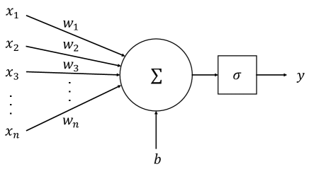
Figure 1: Architecture of a neuron.

The activation function $\sigma$ introduces nonlinear operations into neurons. Otherwise, the structure of neurons will simply be a superposition of linear operations, and the power of the network will be greatly reduced. Activation function $\sigma$ comes in many forms Nwankpa et al. (2018). In this paper, we use the most commonly used activation function ReLU Nair and Hinton (2010) in our study,

$$\sigma(x)=\begin{cases}x\,,&x>0\,,\\ 0\,,&x\leq 0\,.\end{cases}$$ (2)

In general, the current neuron will only output positive values after calculating the weighted sum of data from the first $N$ neurons. From the feature level, it can be understood as the following. After a linear combination of $N$ features, neurons input the combined features into the activation function to obtain the output features.

II.2 Neural Network

The simplest example of neural network is Fully Connected Neural Network (FCNN). The structure of FCNN is shown in Fig. 2. A manually specified number of neurons constitute each layer, which is called a “Dense Layer” of the network. Neurons between different layers are independent. Each neuron receives data from the former layer, calculates the result, and puts them into all neurons of the next layer Hopfield (1982). Note that the input data size has a linear relationship with the parameters of the first layer in FCNN Goodfellow et al. (2016). With the input data size increases, the number of parameters in the network will increase correspondingly, slowing down the learning speed of the model and increasing the requirement of data storage Schmidhuber .

Figure 2: Structure of a FCNN.

Neural network is a supervised learning algorithm, whose characteristic is to use the labeled data—which is the correct output $y$—for training, and test the model on unlabeled data. A loss function is defined to measure the difference between the model output $\hat{y}$ and the correct $y$. The expectation for training is to make the value of loss function as small as possible Goodfellow et al. (2016). The parameters to be informed in the neural network are the weights $\boldsymbol{w}$’s and biases $b$’s in each layer of neurons. According to the gradient descent strategy, parameters in the neural network are updated to the direction where the value of loss function decreases Sra et al. . The gradient descent strategy reads,

$$\theta^{\rm new}=\theta^{\rm old}-\alpha\triangledown_{\theta}J(\theta)\,,$$ (3)

where $\theta$ is the parameter to be updated, $J$ is the loss function, and $\alpha$ is the manually specified learning rate which controls the speed of parameter updates.

The learning of neural network is based on the training dataset collected and annotated by human beings. However, when we finally apply the model to real tasks, we hope the neural network to have good generalization ability. Generalization ability with respect to the neural network is defined as the ability of the network to handle unseen patterns Urolagin et al. (2011). In other words, this concept measures how accurately an algorithm is able to predict outcome values for previously unseen data Mohri et al. . The testing set is a good type of unseen data. The data characteristics of the testing set are similar to the training set. In the meantime, its distribution is independent of the training set, and it does not appear in the training process Goodfellow et al. (2016). Therefore, the final result of the testing set is a reliable index to evaluate the performance of the neural network.

However, if the number of parameters in the network is more compared to the samples in the training set, overfitting occurs Lawrence and Giles (2000). If there are too many parameters in the neural network, the predicting power of the model will get too strong, which makes the model fit the (noisy) characteristics of the training dataset too much in the learning process. As a result, the model is only effective for the data samples that appear in the training set, resulting in the so-called the overfitting problem Hawkins . Therefore, how to design the model structure of neural network with appropriate layers and neuron numbers with strong data generalization ability is an outstanding issue.

II.3 Convolutional Neural Network

As shown in Fig. 3, the structure of CNN is divided into the convolutional layer, the pooling layer, and the dense layer Goodfellow et al. (2016). Each convolutional layer is composed of a specified number of kernels. Each kernel multiplies the input feature values with weights, and adds the biases to obtain outputs. Different kernels get different parameter values after training. The pooling layer itself does not contain any parameters. Take the max-pooling layer as an example. After receiving the input data, this layer scans the data according to a specified stride within a window of a certain length. Then, it outputs the maximum value of the data in each scanning window Yamaguchi et al. (1990). Therefore, the pooling layer compresses the data. It checks all the features in the scanning window and chooses the most important one Ciregan et al. (2012). There are other pooling methods, e.g., the average pooling, which outputs the average value of the data in the window Aghdam and Heravi (2017).

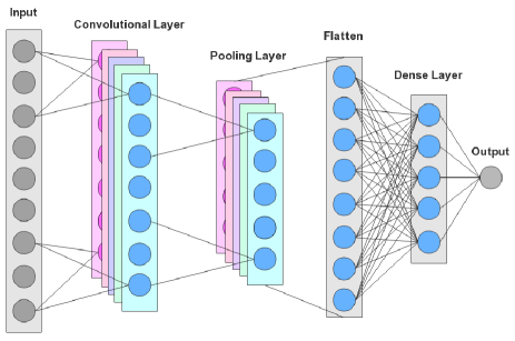
Figure 3: Structure of a CNN.

The pooling layer plays an important role in improving the receptive field of CNN. After the data passes through the pooling layer, the original data length gets shortened, and the kernel in the next convolutional layer can handle a larger range of data than the convolution window in the previous layer, thereby it expands the convolutional layer’s overall operation range of the data Krizhevsky et al. (2017). After extracting the features of the input data through convolutional layers and pooling layers, the flattened feature map will be put into the fully connected layer to obtain the final output Goodfellow et al. (2016).

Since the parameters to be learned by the convolutional layer are only the parameter values in the convolution kernel, they are independent of the input data size. Therefore, CNN reduces the number of free parameters, allowing the network to be deeper with fewer parameters Aghdam and Heravi (2017). Due to its unique model structure and powerful data processing capability, CNN is being widely used Goodfellow et al. (2016).

III Simulated Dataset

In this section we discuss our strategy to simulate GW data and build different datasets for machine learning studies.

III.1 Data Obtaining

Usually, GW waveforms are divided into three stages: inspiral, merger, and ringdown. The signal detected by a single GW detector is,

$$h(t)=F^{+}(t)\,h_{+}(t)+F^{\times}(t)\,h_{\times}(t)\,,$$ (4)

where $h_{+}$ and $h_{\times}$ are two polarization modes of GWs, $F^{+}$ and $F^{\times}$ are the corresponding pattern functions of these two polarization modes as functions of the sky localization and the polarization angle Cutler and Flanagan (1994).

In this work, we focus on GW signals generated by BBH mergers. We use the effective-one-body numerical-relatively (EOBNR) model with aligned spins Bohé et al. (2017) to simulate the waveform. Without losing generality, in addition to the SNR of GW signals, we focus on intrinsic parameters, i.e. masses and spins. The extrinsic parameters, such as the polarization angle and the sky localization, are all fixed to fiducial values. The possible precession effect of BBHs is not considered, since we are using the aligned-spin waveform. The spin parameter is denoted by $\chi$. We set the luminosity distannce $D_{\rm L}=100\,{\rm Mpc}$, and neglect the redshift effect of the GW signal. Such a setting makes us focus on the machine learning algorithm, and the assumptions can easily be relaxed when needed. Worth to mention that, in practice we have tested the effects brought by the inclusion of extrinsic parameters, such as sky location of the GW source, inclination of the BBH orbit, and the polarization angle of the GW. Consistent optimization effects were obtained with extrinsic parameters. Because the dependence of the GW waveform on extrinsic parameters is much simpler than that of intrinsic parameters for GWs from spin-aligned BBHs, in the following we will focus on the intrinsic parameters. It is straightforward to augment with extrinsic parameters in our machine learning data analysis.

We use the open-source tool provided by Gebhard et al. (2019) to generate data. This tool generates GW signals based on PyCBC Nitz et al. (2020) and LALSuite platforms. With given parameters, analog signals from LALSuite contain two time series, i.e. the two polarization modes of GW signals. The above sequences are combined with the corresponding antenna functions $F^{+,\times}$ according to Eq. (4). The signal offset caused by the distance difference between LIGO’s Hanford and Livingston detectors is properly introduced.

The final GW signal sequence used is,

$$s(t)=h(t)+n(t)\,,$$ (5)

where $h(t)$ is the GW waveform obtained by the above simulation (4), and $n(t)$ is the detector’s noise to the strain. The advanced LIGO’s (aLIGO’s) power spectral density (PSD) at the “zero-detuned high-power” design sensitivity (aLIGOZeroDetHighPower) D.Shoemaker (2010) is used to simulate the Gaussian white noise. After inserting the analog waveform into the noise, we can calculate the SNR of the strain. A rescaling of it, corresponding to a rescaling in the distance, can achieve other desired SNR values Cutler and Flanagan (1994). Finally, we get the GW strain with specific SNR values. The strain needs to be preprocessed before being used as the final data, which is similar to PyCBC’s GW data processing. Preprocessing stage includes two steps. The first one is data whitening. The aLIGO’s design sensitivity is used to whiten the original strain, and to filter out the spectral components of the environmental noise so as to properly scale its influence on the strain. The second step is filtering. We filter out the frequency components below 20 Hz to eliminate the influence of the Newtonian noise in the low frequency.

III.2 Dataset Building

This work involves experiments on multiple datasets which have the same structure. They have the following characteristics: (i) with the given parameter range, the data parameters, masses $m_{1,2}$ and spins $\chi_{1,2}$, are all in the form of random sampling; (ii) the ratio of the samples containing the GW signal and pure noise in the dataset is 1 to 1; (iii) the duration of each sample is 1 second, and the sampling rate is 4096 Hz, that is, each sample is a time series with a length of 4096; (iv) considering the symmetry of mass parameters in a BBH, we use $m_{1}\geq m_{2}$ convention to sample masses; (v) the time-series data of the samples all use the Hanford detector sequence (the H1 sequence); (vi) in this work we do not consider the influence of sky position of the GW signal in the strain, that is to say, the peak value of the GW signal is located in the same position of the strain in the datasets. These specifics are natural for a study of such kind.

Totally, we construct 5 datasets for training and 5 datasets for testing, which are annotated as Training Datasets and Testing Datasets hereafter.

• Training Datasets. Each Training Dataset is consisted of a training set and a testing set. The training set and the testing set contain 5000 and 500 samples respectively. When we train the model on each dataset, the model is first trained on the training set, and then tested on the testing set.

• Testing Datasets. Testing Datasets contain many sub-testing sets (annotated as sub-datasets below) to test the model performance on different parameter ranges. Each sub-dataset contains 500 samples.

Table 1: Parameters for Training Datasets.

Dataset	$m_{1}$ $(M_{\odot})$	$m_{2}$ $(M_{\odot})$	$\chi_{1,2}$	SNR
1.1	$[10,80]$	$[10,80]$	0	$[7,7.5]$
1.2	$[10,80]$	$[10,80]$	0	$[7,15]$
2.1	$[30,60]$	$[30,60]$	0	8
3.1	30	45	$[-0.5,0.5]$	8
4.1	$[10,80]$	$[10,80]$	$[-0.998,0.998]$	$[7,15]$

The parameters for Training Datasets used in this work are shown in Table 1. Taking Dataset 1.1 as an example. This dataset only considers three parameters: component masses of the BBHs, $m_{1}$ and $m_{2}$, and the SNR $\rho$. The spin parameters of the BBHs are set to zero. The mass range of both black holes is $m_{i}\in\left[10\,M_{\odot},80\,M_{\odot}\right]$ $(i=1,2)$, and the range of SNR is $\rho\in\left[7,7.5\right]$. The training set has 5000 samples in terms of physical parameters, including 2500 samples which contain the simulated GW signal and 2500 samples of pure noise. The testing set contains 500 samples, including 250 samples containing the simulated GW signal and 250 pure-noise samples. The mass parameter of each sample is randomly drawn from a given range ($m_{1}\geq m_{2}$ as defaulted), whose distribution is shown in Fig. 4. Figure 5 gives two GW examples from Dataset 1.2 with a large SNR (upper panel) and a small SNR (lower panel).

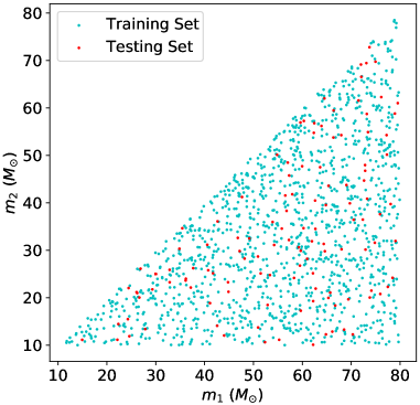
Figure 4: Mass distribution in Dataset 1.1. We use $m_{1}\geq m_{2}$ as a convention to randomly sample mass parameters. Cyan points are the training set samples and red points are the testing set samples.

Table 2: Parameters for Testing Datasets.

Dataset	$m_{1}$ $(M_{\odot})$	$m_{2}$ $(M_{\odot})$	$\chi_{1,2}$	SNR
1	$[10,80]$	$[10,80]$	0	$[7,0.5,15]$
2	$[10,10,80]$	$[10,10,80]$	0	8
3	30	45	$[-0.998,0.25,0.998]$	8
4	$[10,80]$	$[10,80]$	$[-0.998,0.998]$	$[7,15]$
5	$[10,80]$	$[10,80]$	$[-0.998,0.998]$	$[7,0.5,15]$

The parameter settings of Testing Datasets are shown in Table 2. As shown above, the parameters used to construct each sub-dataset are given in the $[{\tt min},{\tt step},{\tt max}]$ format, where ${\tt min}$ and ${\tt max}$ define the overall sampling range of the parameter, and each sub-dataset is constructed with a uniform ${\it step}$ size. Take the Testing Dataset 1 as an example, which consists of 16 sub-datasets. The SNR parameter sampling range of the first sub-dataset is $[7,7.5]$. Each parameter is randomly sampled within this range, and the number of samples is 500. The Testing Dataset will be used to investigate the detection ability of the model in different parameter intervals and explore model robustness with the change of parameter values.

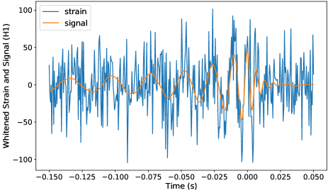
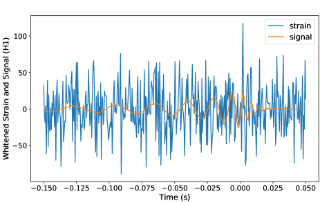
Figure 5: Examples for the simulated GW strain: $(m_{1},m_{2})=(75.61\,M_{\odot},18.64\,M_{\odot})$ and $\rho=14.56$ (upper); $(m_{1},m_{2})=(67.98\,M_{\odot},27.73\,M_{\odot})$ and $\rho=7.41$ (lower). The orange line is the normalized GW signal in the sample strain.

IV Improving Techniques

IV.1 Model Baseline

After preliminary experiments with parameters on networks with different depths and hyperparameter values, we decide to use the network structure similar to that of George and Huerta (2018) as the baseline CNN model. Its structure is shown in Fig. 6.

The model receives GW strain as input and outputs the discriminant value of classification. In the model, the classification threshold is set to 0.5, that is, a sample with a discriminant value greater than 0.5 is judged as a positive sample (i.e., containing a GW signal), otherwise it is judged as a negative one (i.e., pure noise). The baseline model contains three convolutional layers. The number of channels of each convolutional layer is 16, 32, and 64, and the size of the convolution kernel for them is 16, 8, and 8, respectively. After each convolutional layer, a pooling layer and an activation layer are provided. The pooling layer uses maximum pooling with a pooling window of 4 and a step size of 4, which means that the feature sequence is down-sampled to a quarter of the original sequence length and retains the feature with the largest value. The active layer uses the ReLU function shown in Eq. (2). Subsequently, the feature sequences extracted by the convolution structure are input to the fully connected layer to achieve discriminative classification. The model outputs discriminant values to determine whether the sequence contains a GW signal.

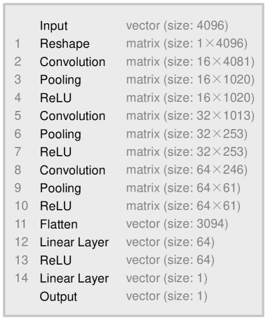
Figure 6: Basic CNN model architecture that is used in this work George and Huerta (2018).

In this work, cross entropy is used as the loss function to update the gradient. Cross entropy is an important concept proposed by Shannon (1948) in information theory. It is often used to measure the difference between the predicted distribution and the true distribution Shannon (1948). Let the label of each sample be $y$ and the discriminant value given by the model be $p$. The cross entropy is,

$$J=-\big{(}y\cdot\log p+(1-y)\cdot\log(1-p)\big{)}\,.$$ (6)

We use ADAM Kingma and Ba (2014) as a gradient descent strategy to update our model parameters. This strategy inputs the samples into the model in batches to calculate the gradient and updates the parameters. After trying batch number values of 5, 10, 25, 50, 100, 200, 250, and 500, we take the value 25, on which the model has the highest accuracy. The learning rate is set to $5\times 10^{-5}$, and the training rate is reduced 10 times every 20 epochs to avoid overfitting the model.

The code implementation of our work is based on the Pytorch framework Paszke et al. (2019), which uses the CUDA deep learning library (cuDNN) Chetlur et al. (2014) to accelerate the GPU’s model operation. Our work deploys experiments on NVIDIA TITAN X GPU.

IV.2 Improving Techniques

We now discuss several improvements—dropout, batch normalization, and the $1\times 1$ convolution—that we experiment on the model of George and Huerta (2018).

Dropout was first proposed by  Hinton et al. (2012) in 2012 to improve the overfitting problem of neural networks. Subsequently, dropout has become one of the widely used techniques in deep learning Srivastava et al. (2014). Its basic idea is that, in each batch of training, the probability $p$ is artificially specified, so that the neurons in the fully connected layer stop working with the probability $p$, and set their parameter values are set to zero.

The advantages of dropout are the following Hinton et al. (2012). First, in the training process of each batch, because the neurons of each layer are inactivated with probability $p$, the network structure of each training is different. The overall model training is equivalent to the joint decision-making process between multiple neural networks with different structures, which helps to improve the problem of overfitting. Second, dropout results in that, two neurons do not necessarily appear in the same network structure each time so that the parameter update no longer depends on the joint decision of some neurons with fixed relationships. At the feature level, this technique prevents decision-making from over-dependence on certain features and forces the model to learn more robust feature representations Goodfellow et al. (2016).

Batch normalization is a neural network training technique proposed by Ioffe and Szegedy (2015) in 2015. Its specific idea is the following. In the training process of each batch, after the data passes through the activation layer, the activation value of each batch of data is normalized. That is, the average value of the sample data of each batch is normalized to 0, and the variance is normalized to 1. In a batch of data of length $m$, the activated data are set to $\mathcal{B}=\left\{x_{1},\cdots,x_{m}\right\}$, and the batch normalized data are set to $\boldsymbol{y}=\left\{y_{1},\cdots,y_{m}\right\}$. Then the batch normalized algorithm is expressed as Ioffe and Szegedy (2015)

$$\mu_{\mathcal{B}} \leftarrow\frac{1}{m}\sum_{i=1}^{m}x_{i}\,,$$ (7)

$$\sigma_{\mathcal{B}}^{2} \leftarrow\frac{1}{m}\sum_{i=1}^{m}\left(x_{i}-\mu_{\mathcal{B}}\right)^{2}\,,$$ (8)

$$\widehat{x}_{i} \leftarrow\frac{x_{i}-\mu_{\mathcal{B}}}{\sqrt{\sigma_{\mathcal{B}}^{2}+\epsilon}}\,,$$ (9)

$$y_{i} \leftarrow\gamma\widehat{x}_{i}+\beta\,,$$ (10)

where $\gamma$ and $\beta$ in the algorithm are the parameters learned in the gradient update. The purpose of this step is to make the result of batch normalization be the same as the original input data, which maintains a possibility to retain the original structure. The parameter $\epsilon$ in Eq. (9) is used to prevent invalid calculation when the variance $\sigma_{\mathcal{B}}^{2}$ is zero.

The batch normalization technique makes the mean and variance of the input data distribution of each layer in the CNN within a certain range. Thus, each layer of the network does not need to adapt to the change in the distribution of input data, which is conducive to accelerating the learning speed of the model and speeding up the simulation Goodfellow et al. (2016). At the same time, batch normalization suppresses the problem that small changes in parameters are amplified with the deepening of the network layers, making the network more adaptable to model parameters and more stable gradient updates. Besides, due to the use of dropout technique, the number of effective neurons in the model decreases, and the fitting speed of network slows down Ioffe and Szegedy (2015). Considering that batch normalization has a significant improvement effect on the fitting speed of the model, dropout and batch normalization techniques are often introduced into the structure of the neural network at the same time Li et al. .

The $1\times 1$ convolution, also known as “network in network”, was proposed by Lin et al. (2013) in 2014. The $1\times 1$ convolution is a convolution kernel of size $1\times 1$. In one-dimensional convolution, it is a convolution kernel in which the window length is 1. The $1\times 1$ convolution is similar to the traditional convolutional layer. After receiving the input data, the operation is gradually performed to obtain the output feature map representation. Its setting parameters commonly used are the number of input channels and the number of output channels Paszke et al. (2019). The number of input channels is the feature dimension of the original data. The number of output channels is the same as the number of convolution kernels, which is the feature dimension of the output data.

The $1\times 1$ convolution recombines multi-dimensional features of the original data without changing the length of them. It enhances the model’s ability to express data features Lin et al. (2013). In addition, if the number of input channels is fewer than the number of output channels, then the $1\times 1$ convolution can be seen as an ascending dimension operation of the original data to increase the feature dimension. This is similar to the effect of data passing through a fully connected layer. Through $1\times 1$ convolution, the interaction and reorganization of multi-dimensional features of the original data are realized, and the model’s ability to represent data features is enhanced Goodfellow et al. (2016).

V Simulation Results

Table 3: The extended techniques used for each model.

Model	Dropout	Batch norm.	$1\times 1$ conv.
ConvNet1
ConvNet2	$\surd$
ConvNet3		$\surd$
ConvNet4			$\surd$
ConvNet5	$\surd$	$\surd$
ConvNet6	$\surd$	$\surd$	$\surd$

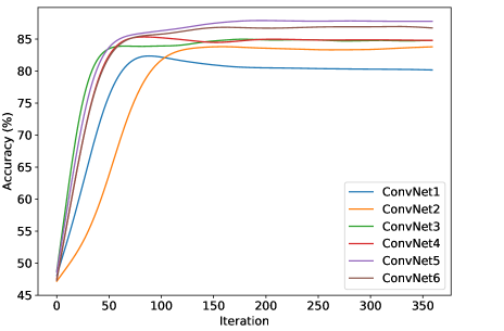
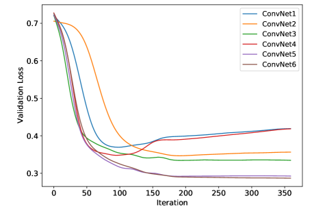
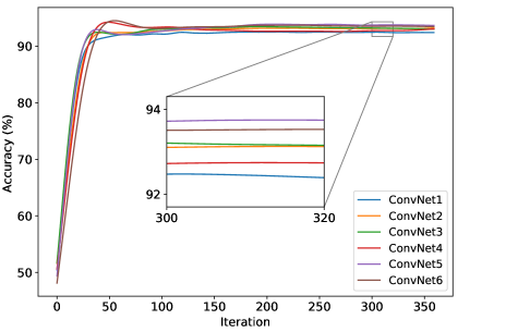
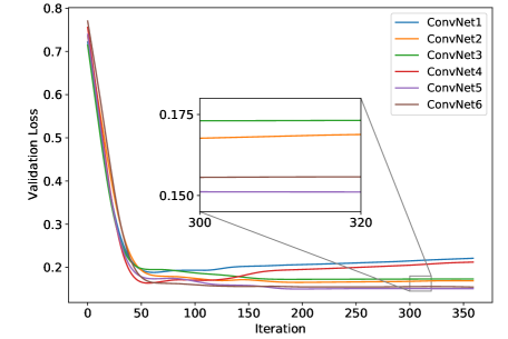
Figure 7: Model comparison on Datasets 1.1 (upper panels) and 1.2 (lower panels). ConvNet1 to ConvNet6 are the models shown in Table 3. We use the accuracy (fraction of samples correctly classified) and the validation loss (loss function value in the validation set) as our metrics to track the model performance in the training process.

Based on the enhanced techniques, we extend the basic model of CNN described in Sec. IV.1. Dropout, batch normalization, and the $1\times 1$ convolution are successively added to the basic model. We test these models with Datasets 1.1 and 1.2. In the Dataset 1.1, the SNR range of GW signals is $\rho\in[7,7.5]$, which makes the signal hard to be detected, representing the edge cases for detection on low SNR signals. The SNR range of Dataset 1.2 is $\rho\in[7,15]$, reflecting the detection capability of the model with relatively loud events. The extended models are shown in Table 3. Considering that dropout and batch normalization have complementary performance in the overfitting problem, we combine these two techniques in our multi-technique models.

The training set and the testing set of the model are based on Datasets 1.1 and 1.2 of Training Datasets described in Sec. III.2. Model parameters and learning strategies are consistent with Sec. IV. We divide 500 samples from the training set as the validation set, which is used to verify the model effect during the training process. When the validation set is input into the model, it does not participate in the gradient update, but is only used to calculate the accuracy and loss function value.

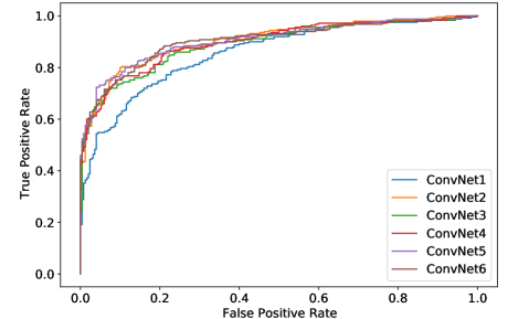
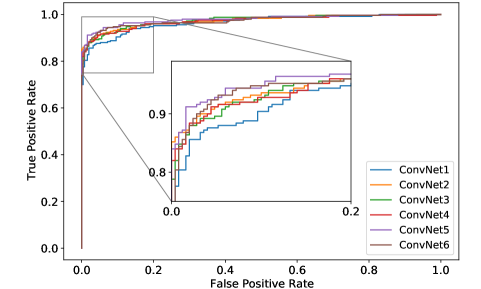
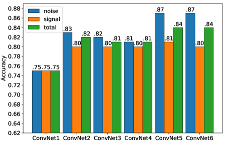
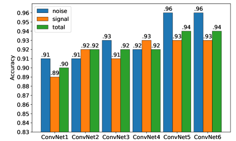
Figure 8: Results on the testing sets of Datasets 1.1 (left panels) and 1.2 (right panels). We use both ROC and the accuracy as our evaluation metrics. As seen in lower panels, the accuracy in identifying noise and signal, as well as the total accuracy, are illustrated separately.

Table 4: AUC scores on Dataset 1.1 and 1.2. The highest value in each column is highlighted.

Dataset	1.1	1.2
ConvNet1	0.86	0.96
ConvNet2	0.90	0.97
ConvNet3	0.89	0.97
ConvNet4	0.90	0.97
ConvNet5	0.91	0.98
ConvNet6	0.91	0.97

The validation results of each model in the training process are shown in Fig. 7. As shown in the figure, based on Dataset 1.1 (low SNR), the accuracy of each extended network model is significantly improved compared with that of the basic model (ConvNet1). The validation results show that the final accuracy of each network is stable at $83\%$–$87\%$, while the accuracy of the basic model is below $80\%$. Among them, ConvNet5, which uses dropout and batch normalization, achieves the highest accuracy in the stable stage after enough iterations. ConvNet6, which uses all improving techniques—namely dropout, batch normalization, and $1\times 1$ convolution—has an accuracy slightly lower than ConvNet5. ConvNet4, which only uses the $1\times 1$ convolution, achieves a high accuracy similar to ConvNet6 in the early stage of training, but decreases later on.

Observing the change in the value of the loss function of the validation set, we find that, in the stable stage, ConvNet6 reaches the lowest value in loss, and the loss of ConvNet5 is slightly higher than ConvNet6. Similarly, the minimum values of the loss function of extended models are all smaller than that of the basic model (ConvNet1). Specifically, after applying the dropout to the model, the decline of the loss function values of ConvNet2 is significantly later than the basic model, and in the stable stage, the validation loss of ConvNet2 is lower than that of the basic model. This shows that the dropout technique indeed slows down the fitting speed of network and reduces the overfitting problem. The loss function value of ConvNet3 with batch normalization decreases faster. This means that the fitting speed of the model is accelerated. At the same time, its loss in validation in the late training stage is relatively stable. ConvNet4 with the $1\times 1$ convolution has a faster fitting speed among the extended models with a single technique, but its late-stage model performance is unstable. In addition, it has the overfitting problem similar to the basic model. ConvNet5 with dropout and batch normalization, and ConvNet6 which uses all three techniques, perform similarly. They both achieve the optimal results in the stable stage. ConvNet6 performs slightly better than ConvNet5 in the stable stage of training.

In Dataset 1.2, the SNR of the GW signal is larger than that in Dataset 1.1, which makes the signal detection much easier and reduces the difference between models. In this situation, the extended model is still superior to the basic model. In terms of accuracy, ConvNet5 reaches the optimal value in the stable stage of the late training epoch. Its performance is slightly better than that of ConvNet6. In terms of the value of loss function, ConvNet5 and ConvNet6 have similar results in the stable stage. Actually, ConvNet5 is slightly better than ConvNet6 in the stable stage. In addition, as the SNR distribution range of the dataset expands, the differences between the samples increase so that the overfitting problem of the model is reduced.

After training, the models are provided to the testing sets for final evaluation. The testing results are shown in Fig. 8. ROC curve is a graphical plot that illustrates the diagnostic ability of a binary classifier system as its discrimination threshold is varied Fawcett ; see Sec. IV.1. When the threshold changes, the curve reflects the fraction of positive samples correctly identified (True Positive Rate) versus the fraction of negative samples incorrectly identified (False Positive Rate) Powers (2008). The area under the curve (annotated as AUC) is equal to the probability that a model ranks a randomly chosen positive sample higher than a negative one Fawcett .

The AUC scores of different models on Datasets 1.1 and 1.2 are shown in Table 4. It can be seen that on Dataset 1.1, ConvNet5 ans ConvNet6 both achieve the highest accuracy and AUC score, but the classification rate of GW signals of ConvNet6 is slightly lower than that of ConvNet5 (shown in Fig. 8). On Dataset 1.2, ConvNet5 achieves both the highest accuracy and AUC score.

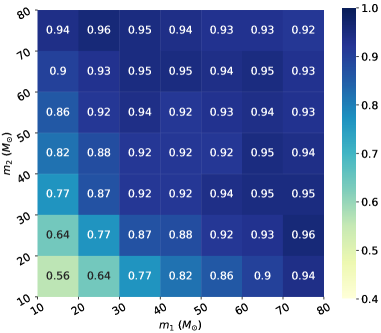
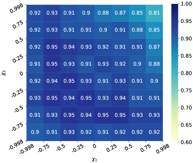
Figure 9: Model robustness on BBH masses (left) and spins (right). The colorbar and numbers are the accuracy of the model tested on different sub-datasets (in specific mass/spin ranges) of Testing Datasets. The mirror part of $m_{2}\geq m_{1}$ is also plotted.

Based on the above study, we find that the dropout, batch normalization, and $1\times 1$ convolution techniques can improve the performance of the basic model of CNNs George and Huerta (2018). Among them, the extended model using multiple techniques achieve better results than using a single technique extension. In this work, ConvNet5 using dropout and batch normalization achieves satisfactory results on both datasets. Therefore, we will use this model in the following analysis.

VI Generalization and Robustness

In the work of George and Huerta (2018), who firstly introduced the CNN structure into the field of GW data processing, the generalization ability of deep learning algorithms in the task of GW signal detection was discussed. Subsequent studies have pointed out that this ability is a major advantage of deep learning algorithms over the matched filtering Gabbard et al. (2018); Gebhard et al. (2019). As mentioned in Sec. II.2, generalization ability refers to the ability of the detection algorithm to respond to signals that are outside of the distribution of training data Mohri et al. . We here are the first to study the generalization ability of the CNN model in the task of GW signal detection, including the generalization characteristics of the CNN model in multiple parameter ranges such as masses and aligned spins.

From the discussion in Sec. V, we use ConvNet5 for our following experiments, and hereinafter we refer it as “the model”. Considering that the discussion in Sec. V is based only on the performance of the model on the dataset where spins are set to zero, we conduct a further test on the ConvNet5 model on Dataset 4.1. Dataset 4.1 introduces spin parameters on the basis of Dataset 1.2, which is used to test the overall performance of the model in the GW detection task. After 30 epochs of training on Dataset 4.1, the model reaches an accuracy of $93\%$, which proves that the model still has a good ability to detect GW signals when considering the spin parameters. In the following subsections, we will test the generalization ability of the model in masses, spins, and the generalization ability of the nonspinning model with spinning data.

VI.1 Mass Parameters

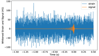
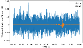
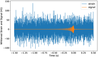
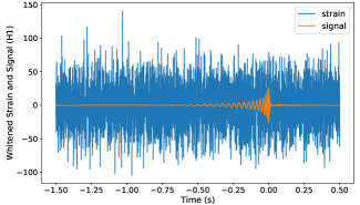
Figure 10: Simulated GW strain examples of different masses and spins. The upper panels are the strain examples of increasing masses from left to right: $(10\,M_{\odot},10\,M_{\odot})$, $(45\,M_{\odot},45\,M_{\odot})$, and $(80\,M_{\odot},80\,M_{\odot})$. The lower panels contain examples of different spins (from left to right): $(0.998,0.998)$, $(0,0)$, and $(-0.998,-0.998)$.

To simplify the investigation, we first study the generalization ability of the model in the GW detection task that only considers mass parameters. The Training Dataset used in this section is Dataset 2.1 (see Table 1). In this dataset, the SNR of the GW signal is 8, the mass sampling range of the BBH is $\left[30\,M_{\odot},60\,M_{\odot}\right]$, and the spins are set to zero. After 30 epochs of training, the accuracy on the testing set is $93\%$. Subsequently, we use the Testing Dataset 2 to test the model on the sub-datasets with the mass sampling range of $\left[10\,M_{\odot},80\,M_{\odot}\right]$. The accuracy is shown in the left panel of Fig. 9.

We find that the model works better on sub-datasets within the original training parameter range of $\left[30\,M_{\odot},60\,M_{\odot}\right]$. For most of sub-datasets beyond the training parameter range (i.e., outside of the range $\left[30\,M_{\odot},60\,M_{\odot}\right]$), high accuracy is still achieved, indicating that the model does have a certain generalization ability in the mass parameter. It can be seen from the data in the figure that the model is more effective for BBHs of high masses, and the accuracy for low-mass BBHs is lower. Studying the signal pattern corresponding to the mass parameter, we find that this is caused by the fact that the model is easier to identify data fluctuations introduced by short signals. As the mass decreases, the GW signal in band becomes longer, which is relatively closer to the characteristics of random noise. This is harder to identify with our CNN model. We show example waveforms of different masses and spins in Fig. 10. It is clear from the upper panels that GW signals of smaller masses are longer, thus they are harder to be detected in our CNN models. We leave the discussion of further improvement of our CNN models in this parameter space to future studies.

VI.2 Spin Parameters

Now we discuss the generalization ability of the model in spin parameters. We use Dataset 3.1 as an illustration. The SNR of this dataset is 8, the masses of the BBH are $30\,M_{\odot}$ and $45\,M_{\odot}$, and the range of the spin parameter $\chi$ is $\chi_{i}\in[-0.5,0.5]$ ($i=1,2$). After 30 epochs of training with the model, the accuracy on the testing set is $92\%$. Similarly, we use Testing Dataset 3 (see Table 2) to test the model on each sub-dataset with the spin parameter $\chi$ ranging in $[-0.998,0.998]$.

The accuracy is shown in the right panel of Fig. 9. Similar to the generalization ability in the mass parameter, the model performs well on the sub-datasets in the original parameter range. It also has good accuracy on the sub-datasets beyond the parameter range. Among them, the model performs slightly worse on the sub-datasets with larger positive spins. This is also consistent with the case in Sec. VI.1. As shown in the lower panels of Fig. 10, the spin parameters of the BBHs are taken as $(0.998,0.998)$, $(0,0)$, $(-0.998,-0.998)$, respectively, from left to right. It is clear that with the increase of the $\chi$ value, the GW signals become longer (the “hang-up” effect), thus harder to be detected with our CNN model. Further improvements in this aspect will be subject to future studies.

VI.3 Robustness of Nonspinning Model on Spinning Data

What if the model is only trained with nonspinning GW signals, and it is tested with spinning signals? We use the Dataset 1.2 (see Table 1) for training that only uses the mass parameters. After 30 epochs of training, we test the model on the Testing Dataset 4 (see Table 2) which contains spin parameters as well. We obtain an accuracy of $\sim 92\%$. The accuracy of the model is only slightly reduced compared to the accuracy of $\sim 94\%$ in the Dataset 1.2 where only the mass parameter is included. It shows the generalization ability of the model that is only trained with nonspinning GWs, but tested in data containing spin parameters.

We further use the Testing Dataset 5 (see Table 2) to test the model on sub-datasets with different SNR distribution. The result is shown in Fig. 11. As shown in the figure, the model has the best detection efficiency on data with high SNR and it is slightly worse on data with low SNR. However, on the sub-dataset of testing data with SNR in the range of $[7.0,7.5]$, the model still maintains an accuracy of $\sim 83\%$. This shows that the CNN model which was trained only with nonspinning data is robust to data containing nonzero spin parameters.

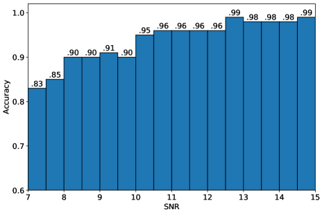
Figure 11: Robustness of CNN models that are only trained with nonspinning GWs on the spinning GW data for different SNRs.

VI.4 Conclusion

From the above study, it can be seen that the CNN model shows good generalization ability for data of different parameter ranges, which is a major advantage over the matched filtering method in using the CNN model. The matched filtering method is based on the existing template bank. Its search and response to GW signals are limited to the existing waveforms. The GW signals beyond the existing waveforms cannot be easily detected. The generalization ability of the CNN model in the task of GW signal detection will help us to discover signals beyond the existing templates. It may also be able to detect signals that imprint orbital eccentricity Liu et al. (2020), orbital precession Babak et al. (2017), and deviations from general relativity Shao et al. (2017). Such a generalization ability will undoubtedly play an essential role in searches of GW signals beyond what we have in the template bank. More studies are needed along this direction.

VII Discussion

For the first time, this work specifically studied the effects on CNN models brought by the improving techniques—such as dropout, batch normalization, and $1\times 1$ convolution—in the task of GW signal detection. Comparisons of models with the combination of different improving techniques were made. Our simplified experiments show that dropout, batch normalization, and the $1\times 1$ convolution can significantly improve the accuracy of the basic model George and Huerta (2018). In addition, we conducted specific experiments and discussed the generalization ability of CNNs in GW signal detection tasks. Experiments show that, the CNN model has good generalization ability over multiple parameter ranges, including masses and aligned spins. It is a major advantage of the deep learning models compared with the matched-filtering method.

In recent years, with the rapid development in the field of deep learning, deep learning models and algorithms have emerged one after another. CNN is only a basic model in the market of deep learning though, it has shown excellent performance in many fields such as image recognition and signal detection Goodfellow et al. (2016). As the difficulty of the task continues to increase, the requirements for feature extraction and processing are getting higher and higher. The network depth of the CNN is limited by the gradient propagation problem, resulting in a limitation on its performance Goodfellow et al. (2016). The proposal of the residual network structure greatly alleviates the problem of gradient propagation in CNNs and makes the depth limit of CNN models rapidly expand He et al. (2016). In the field of time series processing, the “Long Short Term Memory” model is widely used in multiple tasks such as speech processing and stock price prediction, and has achieved excellent results Hochreiter and Schmidhuber (1997). At present, some studies have introduced the above structure into the process of GW data processing Dreissigacker et al. (2019); Shen et al. (2019). However, in the task of GW signal detection, there is still a lack of unified investigation on these models. Comparing these models (including CNN models) on GW signal detection tasks, such as the recognition rate, model size, running time and other indicators, is crucial to find an optimal model structure suitable for real-world task. It is a worthwhile direction for future studies.

For the sake of simplifying the investigation, this work only uses simulated white noise to construct GW sample data. In order to make the model more in line with the characteristics of reality detection, real noise construction from aLIGO/Virgo data can be conducted. At the same time, the data used in this article are only for experimental purposes, so the amount of data is limited. By increasing the number of samples in the dataset, the performance of the model can be further improved. Ensemble learning is also an optimization technique that is worth considering, where the basic idea is to train multiple neural network models, and to use voting and other common decision-making strategies in order to make up for the decision-making defects of a single model and to improve the decision-making ability of the overall model Opitz and Maclin (1999). These aspects deserve detailed studies on their own.