SeasonDepth: Cross-Season Monocular Depth Prediction Dataset and Benchmark under Multiple Environments

Abstract

Different environments pose a great challenge to the outdoor robust visual perception for long-term autonomous driving, and the generalization of learning-based algorithms on different environments is still an open problem. Although monocular depth prediction has been well studied recently, few works focus on the robustness of learning-based depth prediction across different environments, e.g. changing illumination and seasons, owing to the lack of such a multi-environment real-world dataset and benchmark. To this end, the first cross-season monocular depth prediction dataset and benchmark, SeasonDepth, is introduced to benchmark the depth estimation performance under different environments. We investigate several state-of-the-art representative open-source supervised and self-supervised depth prediction methods using newly-formulated metrics. Through extensive experimental evaluation on the proposed dataset and cross-dataset evaluation with current autonomous driving datasets, the performance and robustness against the influence of multiple environments are analyzed qualitatively and quantitatively. We show that long-term monocular depth prediction is still challenging and believe our work can boost further research on the long-term robustness and generalization for outdoor visual perception. The dataset is available on https://seasondepth.github.io, and benchmark toolkit is available on https://github.com/SeasonDepth/SeasonDepth.

1 Introduction

Perception and localization for autonomous driving and mobile robotics have made significant progress due to the boost of deep neural networks [17, 52, 44, 97, 96] in recent years. However, since the outdoor environmental conditions are changing because of different seasons, weather and daytime [56, 70, 53], the pixel-level appearance is drastically affected, which casts a big challenge for robust long-term visual perception and localization. Monocular depth prediction plays a critical role in long-term visual perception and localization [109, 46, 34, 31, 63, 95] and is also significant to safe applications such as self-driving cars under different environmental conditions. Although some depth prediction datasets [14, 66, 1] include different environments for diversity, it is still not clear what kind of algorithm is more robust to adverse conditions and how they influence depth prediction performance. Besides, the generalization of learning-based depth prediction methods on different weather and illumination effects is still an open problem. Therefore, building a new dataset and benchmark under multiple environments is needed to study this problem systematically. To the best of our knowledge, we are the first to study the generalization of learning-based depth prediction under changing environments, which is essential and significant to both robust machine learning algorithms and practical applications like autonomous driving.

The outdoor high-quality dense depth maps are not easy to obtain using LiDAR or laser scanner projection [21, 73, 1, 15], or stereo matching [14, 90, 91], let alone collections under multiple environments. We adopt Structure from Motion (SfM) and Multi-View Stereo (MVS) pipeline with RANSAC followed by careful manual post-processing to build a scaleless dense depth prediction dataset SeasonDepth with multi-environment traverses based on the urban part of CMU Visual Localization dataset [70, 3]. Some examples in the dataset are shown in Fig. 1.

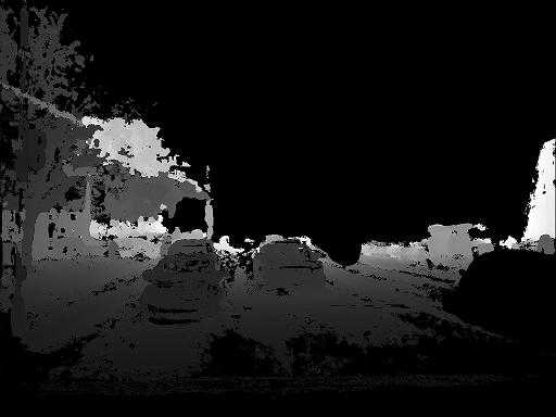
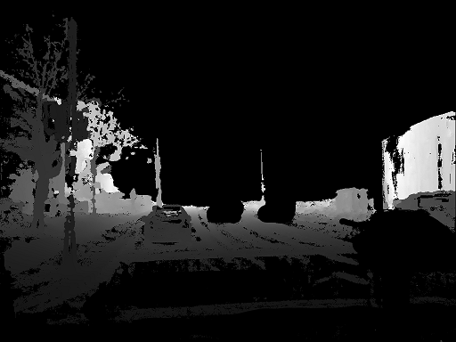
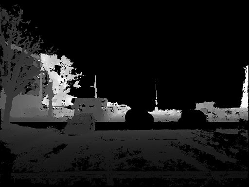
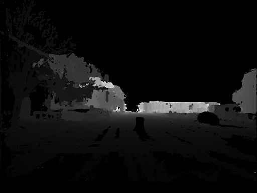
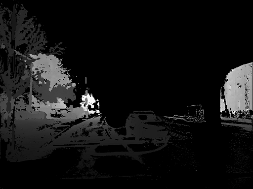
Figure 1: SeasonDepth samples with depth maps under Cloudy + Foliage, Low Sun + Foliage, Cloudy + Mixed Foliage, Overcast + Mixed Foliage and Low Sun + Mixed Foliage.

For the benchmark on the proposed dataset, several statistical metrics are proposed for the experimental evaluation of the representative and state-of-the-art open-source methods from KITTI leaderboard [21, 84]. The typical baselines we choose include supervised [17, 47, 99, 50, 49, 65], stereo training based self-supervised [23, 89, 83], monocular video based self-supervised [110, 25, 22, 67, 40, 108, 88, 92, 37, 98] and domain adaptation [2, 105, 103] algorithms. Through thoroughly analyzing benchmark results, we find that most well-tuned methods cannot present satisfactory performance in terms of both mean and variance under multiple environments. Besides, through cross-dataset evaluations, current KITTI pretrained models cannot generalize well on our dataset while the models tuned on our dataset perform better on KITTI [21] compared to models tuned on Cityscapes [14]. Furthermore, the performance under each adverse environment is investigated both qualitatively and quantitatively to show hints to address robust perception against challenging environments.

For the open problem of generalizability of learning-based depth prediction methods on different environmental conditions, our dataset is the first one that contains real-world RGB images with multiple environments under the same routes so that fair cross-environment evaluation and comparison can be conducted, giving hints to the future research on robust perception in changing environments. In summary, our contributions in this work are listed as follows.

• A new monocular depth prediction dataset SeasonDepth with the same multi-traverse routes under changing environments is introduced through SfM and MVS pipeline and is publicly available to the community.

• We benchmark best and representative open-sourced supervised and self-supervised prediction methods on SeasonDepth using several new statistical metrics.

• From the extensive cross-environment and cross-dataset evaluation, we find that long-term robust depth prediction is still challenging and our dataset and benchmark can give future research direction by pointing out how adversary environments affect the performance with some promising hints to enhance robustness.

The rest of the paper is structured as follows. Sec. 2 analyzes the related work about depth prediction datasets and algorithms. Sec. 3 presents the process of building SeasonDepth. Sec. 4 introduces the metrics and benchmark setup. The experimental evaluation and analysis are shown in Sec. 5. Finally, in Sec. 6 we give the conclusions.

Table 1: Comparison between SeasonDepth and Other Datasets

Name	Scene	Real or Virtual	Depth Value	Sparse or Dense	Multiple Traverses	Different Environments
NYUV2 [77]	Indoor	Real	Absolute	Dense	$\times$	$\times$
DIML [39]	Indoor	Real	Absolute	Dense	$\times$	$\times$
iBims-1 [41]	Indoor	Real	Absolute	Dense	$\times$	$\times$
Make3D [73]	Outdoor & Indoor	Real	Absolute	Sparse	$\times$	$\times$
ReDWeb [90]	Outdoor & Indoor	Real	Relative	Dense	$\times$	$\times$
WSVD [86]	Outdoor & Indoor	Real	Relative	Dense	$\times$	$\times$
HR-WSI [91]	Outdoor & Indoor	Real	Absolute	Dense	$\times$	$\times$
DIODE [85]	Outdoor & Indoor	Real	Absolute	Dense	$\times$	$\times$
OASIS [11]	Outdoor & Indoor	Real	Relative	Dense	$\times$	$\times$
3D Movies [66]	Outdoor & Indoor	Real	Relative	Dense	$\times$	$\checkmark$
KITTI [21]	Outdoor	Real	Absolute	Sparse	$\times$	$\times$
Cityscapes [14]	Outdoor	Real	Absolute	Dense	$\times$	$\checkmark$
DIW [10]	Outdoor	Real	Relative	Sparse	$\times$	$\times$
MegaDepth [50]	Outdoor	Real	Relative	Dense	$\times$	$\times$
DDAD [25]	Outdoor	Real	Absolute	Dense	$\times$	$\times$
MPSD [1]	Outdoor	Real	Absolute	Dense	$\times$	$\checkmark$
V-KITTI [19]	Outdoor	Virtual	Absolute	Dense	$\checkmark$	$\checkmark$
SYNTHIA [68]	Outdoor	Virtual	Absolute	Dense	$\times$	$\times$
TartanAir [87]	Outdoor & Indoor	Virtual	Absolute	Dense	$\checkmark$	$\checkmark$
DeepGTAV [59]	Outdoor	Virtual	Absolute	Dense	$\checkmark$	$\checkmark$
SeasonDepth	Outdoor	Real	Relative	Dense	$\checkmark$	$\checkmark$

2 Related Work

2.1 Monocular Depth Prediction Datasets

Depth prediction plays an important role in the perception and localization of autonomous driving and other computer vision applications. Many indoor datasets are built through calibrated RGBD cameras [77, 39, 41], expensive laser scanners [73, 85] and web stereo photos [86, 90, 91, 66, 43]. However, outdoor depth maps as ground truth are more complex to get, e.g. projecting 3D point cloud data onto the image plane [21, 73, 1] for sparse maps and using stereo matching to calculate inaccurate and limited-scope depth [14, 66, 90]. Another way to get the depth map is through SfM [10, 50, 11, 1] from monocular sequences. Although this method is time-consuming, it generates pretty accurate relatively-scaled dense depth maps , which is more general for depth prediction under different scenarios. For the long-term robust perception under changing environments, though some real-world datasets [14, 1, 66] include some environmental changes, there are still no multi-environment traverses with the same routes, which is essential and necessary for the fair evaluation of robustness across different environments. Since graphical rendering is becoming more and more realistic, some virtual synthetic datasets [19, 68, 87, 59, 81] contain multi-environment traverses. But the rendered RGB images are still different from real-world ones due to the domain gap and cannot be used to benchmark real-world cross-environment performance. The details of the comparison between datasets are shown in Tab. 1 and Sec. 3.2. The closest work to ours is the Ithaca365 [15], where images and point clouds are collected from multiple environments for different perception tasks. But they do not involve the task of monocular depth prediction but only stereo disparity estimation with LiDAR points as ground truth.

2.2 Monocular Depth Prediction Algorithms

The monocular depth prediction task aims to predict the dense depth map in an active way given one single RGB image. Early studies including CRF [93, 101] and other graph models [72, 73, 51] largely depend on man-made descriptors, constraining the performance of depth prediction. Afterward, studies based on CNNs [17, 16, 44, 78, 38] and Transformers [65, 49, 5] have shown promising results for monocular depth estimation. Eigen et al. [17] first predict depth maps using CNN model, while [44] introducing fully convolutional neural networks to regress the depth value. After that, supervised methods for monocular depth prediction have been well studied through normal estimation [99, 42, 60], the supervision of depth maps and stereo disparity ground truth [50, 18, 47, 91, 64]. However, since outdoor depth map ground truth is expensive and time-consuming to obtain, self-supervised depth estimation methods have appeared using stereo geometric left-right consistency [20, 23, 55, 89, 83, 24], egomotion-pose constraint through monocular video [110, 57, 9, 25, 22, 69, 111, 58, 26, 76, 29, 104, 79, 108, 88] and multi-task learning with optical flow, motion and semantics segmentation [100, 112, 67, 40, 37, 48] inside monocular video training pipeline as secondary supervisory signals. Furthermore, some problems posed by self-supervised learning strategies, such as dynamic objects[71, 48, 12], and scale consistency[102, 6, 7, 35], have also been well studied. Besides, to avoid using expensive real-world depth ground truth, other algorithms are trained on synthetic virtual datasets [19, 68, 87, 59] to leverage high-quality depth maps with zero cost. Such methods [105, 2, 13, 103, 8, 27] confront the domain adaptation from synthetic to real-world domain only supervised by virtual images for model training.

3 SeasonDepth Dataset

Our proposed dataset SeasonDepth is derived from CMU Visual Localization dataset [3] through SfM algorithm. The original CMU Visual Localization dataset covers over one year in Pittsburgh, USA, including 12 different environmental conditions. Images were collected from two identical cameras on the left and right of the vehicle along a route of 8.5 kilometers. And this dataset is also derived for long-term visual localization [70] by calculating the 6-DoF camera pose of images with more appropriate categories about the weather, vegetation and area. To be consistent with the content of driving scenes in other datasets like KITTI, we adopt images from Urban areas categorized in [70] to build our dataset. More details about the dataset can be found in Appendix Sec. A.

3.1 Dense Reconstruction and Post-processing

We reconstruct the dense model for each traversal under every environmental condition through SfM and MVS pipeline [75], which is commonly used for depth reconstruction [25, 50] and most suitable for multi-environment dense reconstruction for 3D mapping [45, 70] and show advantage on the aspects of high dense quality despite of huge computational efforts compared to active sensing from LiDAR. Specifically, similar to MegaDepth [50], COLMAP [74, 75] with SIFT descriptor [54] is used to obtain the depth maps through photometric and geometric consistency from sequential images.

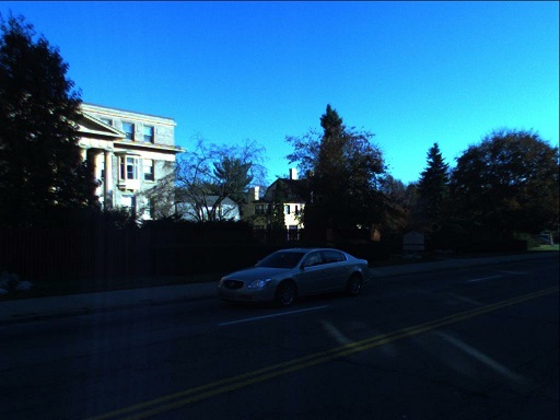
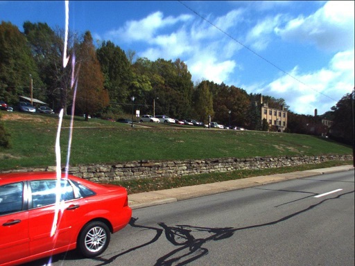
RGB Images

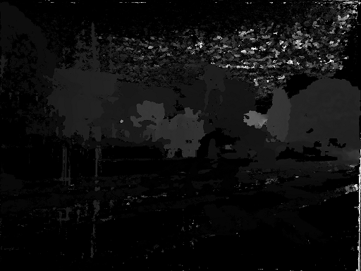
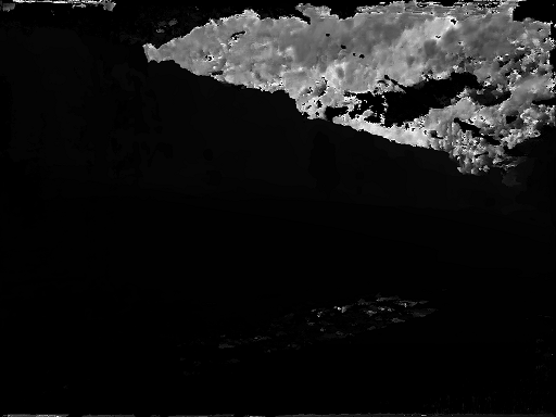
After SfM

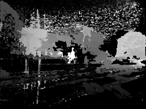
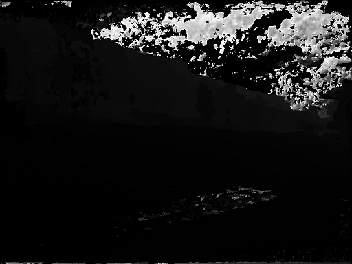
Range Filtering

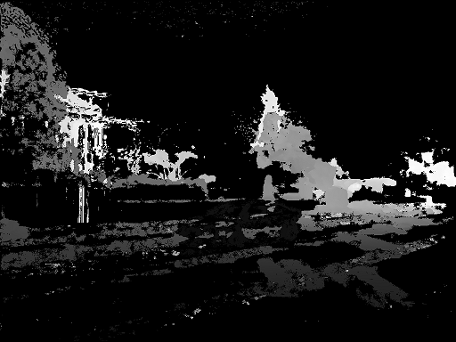
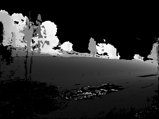
HSV Filtering

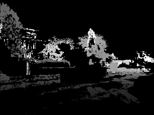
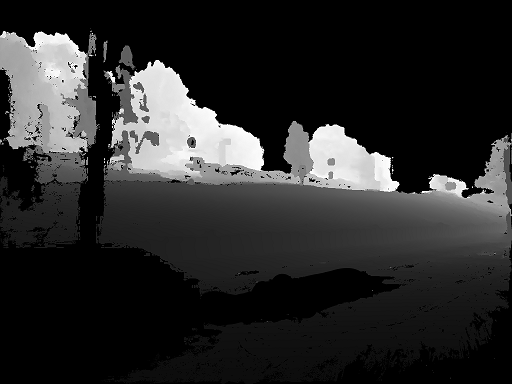
Post-processing

Figure 2: The illustration of depth map processing.

Furthermore, we adopt RANSAC algorithm in the SfM to remove the inaccurate values of dynamic objects in the images through effective modification in SIFT matching triangulation based on the original COLMAP, where dynamic objects with additional motion besides relative camera motion do not obey the multi-view geometry constraint and should be removed as noise via RANSAC in bundle adjustment optimization. Besides, from our justification experiments in Sec. 5.4, it is validated that using relative depth values and removing dynamic noise will not significantly influence the training and the performance of depth prediction models. Because the MVS algorithm generates the depth maps with error pixel values that are out of range or too close, like the cloud in the sky or noisy points on a very near road, we filter those outside the normal range of the depth map.

After the reconstruction, based on the observation of noise distribution in the HSV color space, e.g. blue pixels always appear in the sky and dark pixels always appear in the shade of the low sun, which tend to be noise in most cases, we remove the noisy values in the HSV color space given some specific thresholds. Though outliers are set to be empty in RANSAC, instance segmentation is adopted through MaskRCNN [28] to fully remove the noise of dynamic objects. However, since it is difficult to generate accurate segmentation maps only for dynamic objects under drastically changing environments, we leverage human annotation as the last step to finally check the depth map. The data processing is shown in Fig.2 with normalization after each step. Since we are rigorous and serious to the quality of valid depth pixels which are used for benchmark, we set most noise to be invalid (which causes some “holes” on the boundary from appearance) to avoid any possible pollution to the following benchmark, ensuring the reliable evaluation and benchmark results. More details can be found in Appendix Sec. A.1.

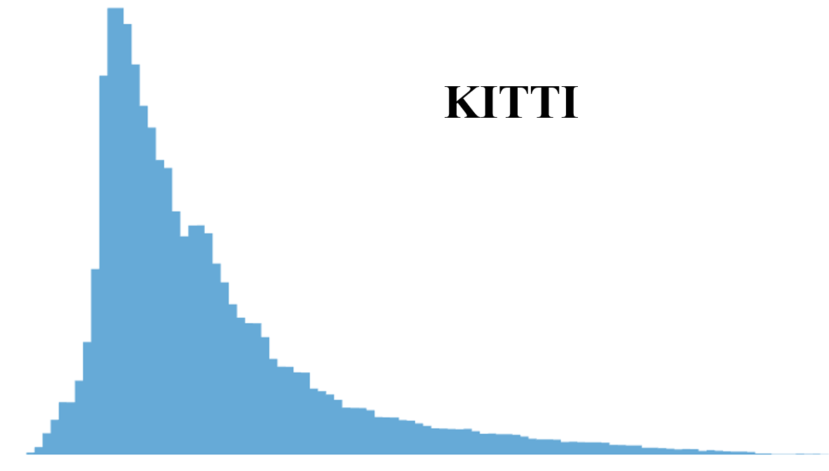
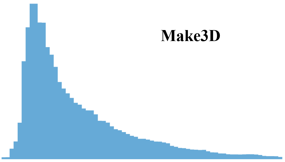
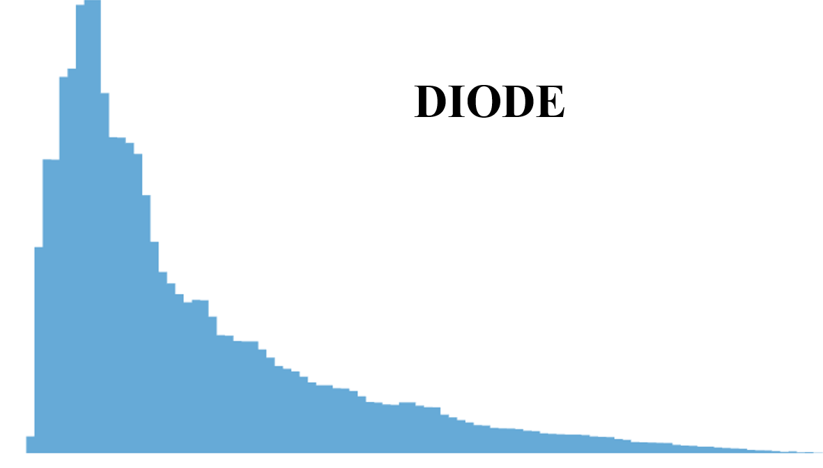
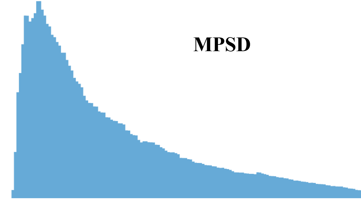
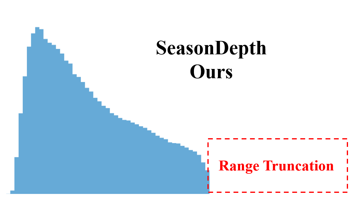
Figure 3: Comparison of relative depth distributions of several datasets.

3.2 Comparison with Other Datasets

The current datasets are introduced in Sec. 2.1. The comparison between SeasonDepth and current datasets is shown in Tab. 1. The distinctive feature of the proposed dataset is that SeasonDepth contains comprehensive outdoor real-world multi-environment sequences with repeated scenes, just like virtual synthetic datasets [19, 59, 87, 81] but they are rendered from computer graphics and suffer from the huge domain gap. Though real-word datasets [1, 66, 14, 80] include different environments, they lack the same-route traverses under different conditions so they are not able to fairly evaluate the performance across changing environments. Similar to outdoor datasets [10, 50, 11], the depth maps of ours are scaleless with relative depth values, where the metrics should be designed for evaluation as the following section shows. The depth map ground truth from SfM is dense compared to LiDAR-based sparse depth maps. Besides, the comparison of depth value distribution is shown in Fig. 3. Note that the values of our dataset are scaleless and relative, so the x-axes of other datasets are also omitted for a fair comparison. We normalize the depth values for all the environments to mitigate the influence of the aggregation from relative depth distributions under different environments to get the final distribution map. The details of implementation can be found in Appendix Sec. A.2. From Fig. 3, it can be seen that our dataset also follows the long-tail distribution [36] which is the same as other datasets, with a difference of missing large-depth part due to range truncation during the building process in Sec. 3.1.

4 Benchmark Setup

4.1 Evaluation Metrics

The challenge for the design of evaluation metrics lies in two folds. One is to cope with scaleless and partially-valid dense depth map ground truth, and the other is to fully measure the depth prediction average performance and the stability or robustness across different environments. Due to the scaleless ground truth of relative depth value, some common metrics [84] cannot be used for evaluation directly. Since the focal lengths of two cameras are close enough to generate similarly-distributed depth values, unlike [110, 50, 11], we align the distribution of depth prediction to depth ground truth via mean value and variance for a fair evaluation. The other key point for multi-environment evaluation lies in the reflection of robustness to changing environments for same-route sequences, which has not been studied in the previous work to the best of our knowledge. We formulate our metrics below.

First, for each pair of predicted and ground truth depth maps, the valid pixels $D^{i,j}_{valid_{predicted}}$ of the predicted depth map $D_{valid_{predicted}}$ are determined by non-empty valid pixels $D^{i,j}_{valid_{GT}}$ of the depth map ground truth. And then the valid mean and variance of both $D_{valid_{GT}}$ and $D_{valid_{predicted}}$ are calculated as $Avg_{GT}$,$Avg_{pred}$ and $Var_{GT}$,$Var_{pred}$. Then we adjust the predicted depth map $D_{adj}$ to get the same distribution with $D_{valid_{GT}}$,

$${D_{adj}}=({D_{pred}}-Av{g_{pred}})\times\sqrt{{{Va{r_{GT}}}\mathord{\left/{\vphantom{{Va{r_{GT}}}{Va{r_{pred}}}}}\right.\kern-1.2pt}{Va{r_{pred}}}}}+Av{g_{GT}}$$

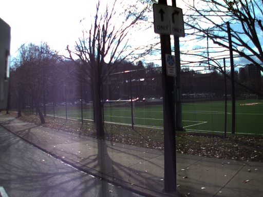
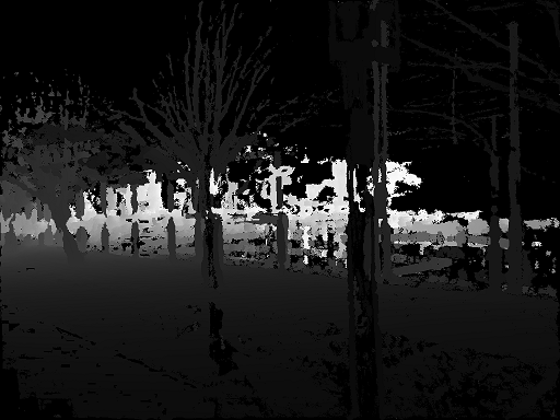
RGB and ground truth

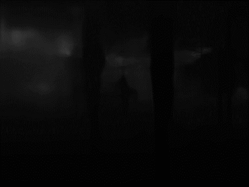
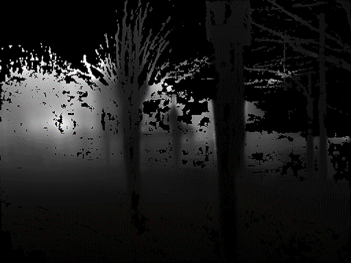
PackNet [25]

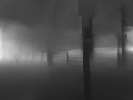
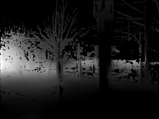
VNL [99]

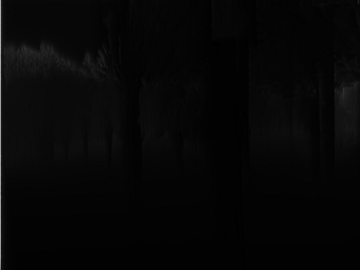
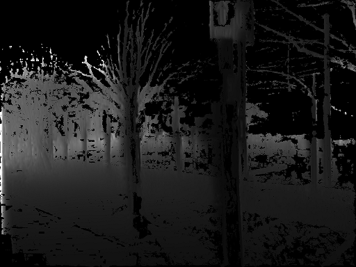
GASDA [103]

Figure 4: The examples of depth adjustment (from the first to second row) for prediction results.

The examples of adjusted depth prediction are shown in Fig. 4. After this operation, we can eliminate scale difference for depth prediction across datasets, which makes this zero-shot evaluation on SeasonDepth reliable and applicable to all the models even though they predict absolute depth values, showing generalization ability on new datasets and robustness across different environments. Denote the adjusted valid depth prediction $D_{adj}$ as $D_{P}$ in the following formulation. To measure the depth prediction performance, we choose the most distinguishable metrics under multiple environments from commonly-used metrics in [84], AbsRel and $\delta<1.25$ ($a_{1}$). For environment $k$, we have,

$$AbsRel^{k}=\frac{1}{n}\sum\limits_{i,j}^{n}{{{\left|{{D_{P}}{{{}^{k}}_{i,j}}-{D_{GT}}{{{}^{k}}_{i,j}}}\right|}\mathord{\left/{\vphantom{{\left|{{D_{P}}{{{}^{k}}_{i,j}}-{D_{GT}}{{{}^{k}}_{i,j}}}\right|}{{D_{GT}}{{{}^{k}}_{i,j}}}}}\right.\kern-1.2pt}{{D_{GT}}{{{}^{k}}_{i,j}}}}}$$

$$a_{1}^{k}=\frac{1}{n}\sum\limits_{i,j}^{n}{\mathbbm{1}(max\{\frac{{D_{P}}{{{}^{k}}_{i,j}}}{{D_{GT}}{{{}^{k}}_{i,j}}},\frac{{D_{GT}}{{{}^{k}}_{i,j}}}{{D_{P}}{{{}^{k}}_{i,j}}}\}<1.25})$$

For the evaluation under different environments, 6 secondary metrics are derived based on original metrics,

$$AbsRel^{avg}=\frac{1}{m}\sum\limits_{k}{{AbsRel^{k}}},a_{1}^{avg}=\frac{1}{m}\sum\limits_{k}{{a_{1}^{k}}}$$

$$AbsRel^{var}=\frac{1}{m}{\sum\limits_{k}{\left|{{AbsRel^{k}}-\frac{1}{m}\sum\limits_{k}{{AbsRel^{k}}}}\right|}^{2}}$$

$$a_{1}^{var}=\frac{1}{m}{\sum\limits_{k}{\left|{{a_{1}^{k}}-\frac{1}{m}\sum\limits_{k}{{a_{1}^{k}}}}\right|}^{2}}$$

where $avg$ terms $AbsRel^{avg}$, $a_{1}^{avg}$ and $var$ terms $AbsRel^{var}$, $a_{1}^{var}$ come from Mean and Variance in statistics, indicating the average performance and the fluctuation around the mean value across multiple environments.

Considering the depth prediction applications, it should be more rigorous to prevent better results fluctuation than worse results under changing conditions. Therefore, we use the Relative Range terms $AbsRel^{relRng}$, $a_{1}^{relRng}$ to calculate the relative difference of maximum and minimum for all the environments.

$$AbsRe{l^{relRng}}=\frac{\max\{AbsRe{l^{k}}\}-\min\{AbsRe{l^{k}}\}}{\frac{1}{m}\sum\limits_{k}{AbsRe{l^{k}}}}$$

$$a_{1}^{relRng}=\frac{\max\{1-a_{1}^{k}\}-\min\{1-a_{1}^{k}\}}{\frac{1}{m}\sum\limits_{k}{(1-a_{1}^{k})}}$$

Relative Range terms for AbsRel and $1-a_{1}$ are more strict than the Variance terms $AbsRel^{var}$, $a_{1}^{var}$ and note that $1-a_{1}$ instead of $a_{1}$ is used to calculate $a_{1}^{relRng}$ to make relative range fluctuation more distinguishable for better methods.

4.2 Benchmark Design and Algorithms

In the experiment, we aim to first benchmark the well-tuned performance on SeasonDepth using state-of-the-art algorithms and then present the cross-dataset performance with other datasets using representative baselines of each category. More details can be found in Appendix Sec. B.1 and B.3.

We first split the split training set, validation set, and test set with 11407, 17225 and 3944 images respectively. Note that the detailed analysis for each environment is based on the validation set which requires more images. For the benchmark on SeasonDepth, though there is no limit to other datasets or pre-trained models to obtain the best performance, since SeasonDepth only has monocular images as the training set, we categorize the state-of-the-art evaluated algorithms as supervised methods and self-supervised methods with monocular video training. Specifically, DepthFormer [49], BTS [47] are DPT [65] are supervised baselines, while SUB-Depth [108],VADepth [92], Monodepth2 [22], SfMLearner [110] and ManyDepth [88] are self-supervised baselines.

Table 2: SeasonDepth Benchmark ($\downarrow$: Lower Better, $\uparrow$: Higher Better, Best for each category)

		Average		Variance$(10^{-2})$		Relative Range
Category	Method	$AbsRel$ $\downarrow$	$a_{1}$ $\uparrow$	$AbsRel$ $\downarrow$	$a_{1}$ $\downarrow$	$AbsRel$ $\downarrow$	$1-a_{1}$ $\downarrow$
	DepthFormer [49]	0.135	0.835	0.0210	0.120	0.294	0.576
	BTS [47]	0.242	0.587	0.0222	0.0632	0.220	0.220
Supervised	DPT [65]	0.152	0.790	0.0286	0.1574	0.364	0.637
	SUB-Depth [108]	0.095	0.920	0.008	0.015	0.398	0.668
	VADepth [92]	0.131	0.852	0.006	0.024	0.247	0.397
	Monodepth2 [22]	0.144	0.824	0.011	0.046	0.305	0.502
	SfMLearner [110]	0.325	0.482	0.107	0.155	0.298	0.236
Self-supervised Monocular Video Training	ManyDepth [88]	0.227	0.649	0.080	0.262	0.486	0.549

Table 3: Cross-dataset Generalization from KITTI to SeasonDepth ($\downarrow$: Lower Better, $\uparrow$: Higher Better, Best for each category)

		KITTI Eigen Split		SeasonDepth: Average		Variance$(10^{-2})$		Relative Range
Category	Method	$AbsRel$ $\downarrow$	$a_{1}$ $\uparrow$	$AbsRel$ $\downarrow$	$a_{1}$ $\uparrow$	$AbsRel$ $\downarrow$	$a_{1}$ $\downarrow$	$AbsRel$ $\downarrow$	$1-a_{1}$ $\downarrow$
	Eigen et al. [17]	0.203	0.702	1.093	0.340	0.346	0.0170	0.206	0.0746
	BTS [47]	0.060	0.955	0.676	0.209	0.545	0.0650	0.405	0.129
	MegaDepth [50]	0.220	0.632	0.515	0.417	0.0874	0.0285	0.200	0.107
Supervised	VNL [99]	0.072	0.938	0.306	0.527	0.126	0.166	0.400	0.290
	Monodepth [23]	0.148	0.803	0.436	0.455	0.0475	0.0213	0.198	0.104
	adareg [89]	0.126	0.840	0.507	0.405	0.0630	0.0474	0.178	0.0137
Self-supervised Stereo Training	monoResMatch [83]	0.096	0.890	0.487	0.389	0.286	0.0871	0.414	0.160
	SfMLearner [110]	0.181	0.733	0.360	0.495	0.0801	0.0628	0.269	0.182
	PackNet [25]	0.116	0.865	0.722	0.421	0.187	0.0705	0.186	0.155
	Monodepth2 [22]	0.106	0.874	0.256	0.624	0.0311	0.0532	0.235	0.229
	CC [67]	0.140	0.826	0.648	0.479	0.223	0.0881	0.280	0.241
	SGDepth [40]	0.113	0.879	0.648	0.480	0.0987	0.0498	0.197	0.169
	FSRE-Depth [37]	0.105	0.886	0.256	0.624	0.0288	0.0283	0.227	0.158
	CADepth-Net [98]	0.105	0.892	0.257	0.625	0.0447	0.0725	0.265	0.278
Self-supervised Monocular Video Training	VADepth [92]	0.104	0.892	0.230	0.667	0.0158	0.0215	0.205	0.179
	Atapour et al. [2]	0.110	0.923	0.687	0.300	0.224	0.0220	0.231	0.0622
	T2Net [105]	0.169	0.769	0.827	0.391	0.399	0.0799	0.286	0.146
Syn-to-real Domain Adaptation	GASDA [103]	0.143	0.836	0.438	0.411	0.121	0.0665	0.271	0.145

For the cross-dataset performance with other datasets, we choose the other two popular autonomous driving datasets KITTI and Cityscapes together with SeasonDepth. To analyze the performance under each environment, we report the results on the validation set of SeasonDepth. We first present generalization performance from KITTI to SeasonDepth. Following the category introduced in Sec. 2.2, some representative baseline models on KITTI leaderboard [84] are chosen to evaluate the performance on the SeasonDepth dataset without fine-tuning. These methods include supervised methods (Eigen et al. [17], BTS [47], MegaDepth [50] and VNL [99]), self-supervised methods with stereo training (Monodepth [23], adareg [89], monoResMatch [83]), self-supervised methods with monocular video training (SfMLearner [110], Monodepth2 [22], PackNet [25], CC [67], SGDepth [40], FSRE-Depth [37] CADepth-Net [98] VADepth [92]), and domain adaptation methods (Atapour et al. [2], T2Net [105], GASDA [103]) trained on the virtual dataset with multiple environments.

We then introduce cross-dataset comparison evaluation to justify that the depth accuracy and the ground truth are good enough for the dataset usage of autonomous driving for model training in spite of the lack of dynamic objects. Specifically, inspired by cross-dataset transfer degradation evaluation in [66], we compare our dataset with the stereo depth dataset Cityscapes [14] in terms of the degraded performance on KITTI dataset after cross-dataset fine-tuning. Based on the pre-trained models on KITTI, we fine-tune BTS [47] and SfMLearner [110] models on SeasonDepth and Cityscapes dataset with the same amount of images for 50 epochs, and evaluate the depth prediction on KITTI validation set using the metrics of $MAE$, $absErrorRel$, $iMAE$, $iRMSE$, $sqErrorRel$ from [84] and report the mean and standard deviation from the last 10 training epochs.

5 Experimental Evaluation Results

5.1 SeasonDepth Benchmark Results

In this section, we present the evaluation results on the test set of SeasonDepth in Tab. 2. The models are well tuned on SeasonDepth training set and have impressive performance on the test set, especially for $Average$ performance. We can see that self-supervised methods do not perform worse than supervised ones after well-tuning. It can be found that DepthFormer [49] and SUB-Depth[108] perform the best on $Average$ but not satisfactory on $Variance$ or $RelativeRange$, showing that even the well-tuned models cannot perform well consistently across different environments. Therefore, there is still a long way to go even for the state-of-the-art methods towards long-term robust depth estimation.

RGB

Ground Truth

BTS[47]
Supervised

VNL[99]
Supervised

Monodepth
S-Sup-S [23]

adareg[89]
S-Sup-S

PackNet[25]
S-Sup-M

Monodepth2
S-Sup-M [22]

SGDepth[40]
S-Sup-M

T2Net[105]
Syn-to-Real

GASDA[105]
Syn-to-Real

Figure 5: Comparison among supervised, self-supervised stereo based (S-Sup-S), self-supervised monocular video based (S-Sup-M) and domain adaptation (Syn-to-Real) methods.

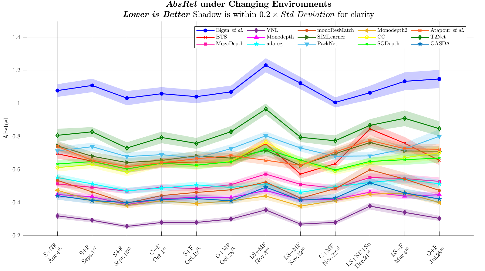
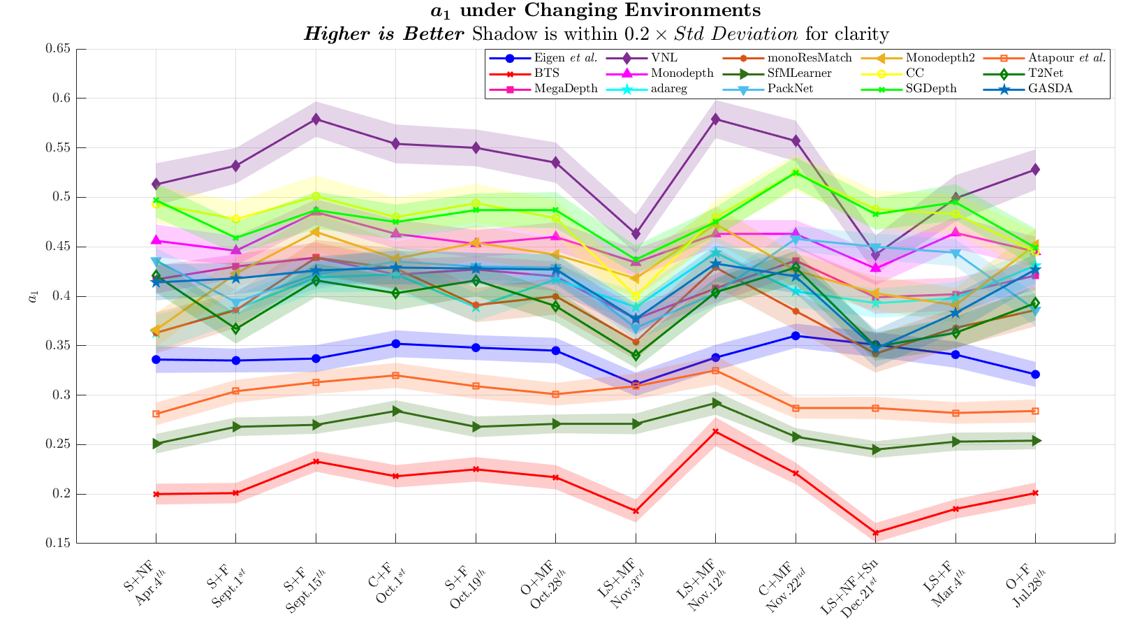
Figure 6: Results on SeasonDepth dataset under 12 different environments with dates. The shadows indicate error bars around mean values with $0.2\times Standard$ $Deviation$ for more clarity.

Table 4: Influence of fine-tuning from KITTI to SeasonDepth
($\downarrow$: Lower Better, $\uparrow$: Higher Better)

	Average		Variance$(10^{-2})$		Relative Range
Method	$AbsRel$ $\downarrow$	$a_{1}$ $\uparrow$	$AbsRel$ $\downarrow$	$a_{1}$ $\downarrow$	$AbsRel$ $\downarrow$	$1-a_{1}$ $\downarrow$
BTS [47]	0.676	0.209	0.545	0.0650	0.405	0.129
BTS [47] (fine-tuned)	0.339	0.479	0.0425	0.0389	0.203	0.117
SfMLearner [110]	0.360	0.495	0.0801	0.0628	0.269	0.182
SfMLearner [110] (fine-tuned)	0.413	0.440	0.0502	0.0290	0.178	0.100

5.2 Cross-dataset Generalization Results

In this section, we show the generalization performance from KITTI to SeasonDepth in Tab. 3. First we can see that in the zero-shot cross-dataset generalization setting, self-supervised methods show more robustness to different environments than supervised ones, which suffer from large values of $Variance$ and $RelativeRange$ and more sensitive. Also, the gap between KITTI results and SeasonDepth $Average$ results is clear, showing that the generalization without fine-tuning is challenging especially in different environments. Interestingly, supervised methods with good $Variance$ performance are not consistent with those with good $Average$ performance, which indicates that algorithms tend to work well in specific environments instead of being robust to all conditions, validating the significance of the cross-environment study with SeasonDepth dataset.

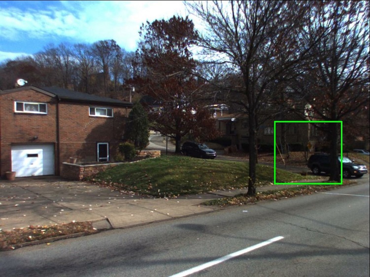
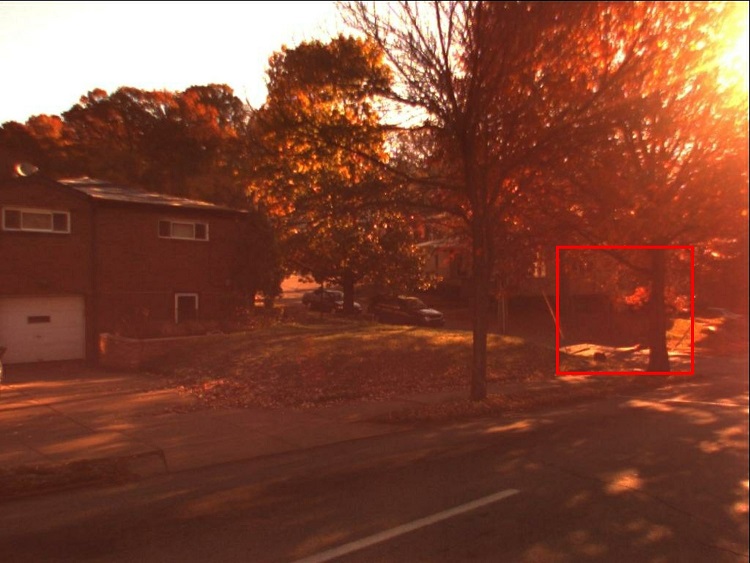
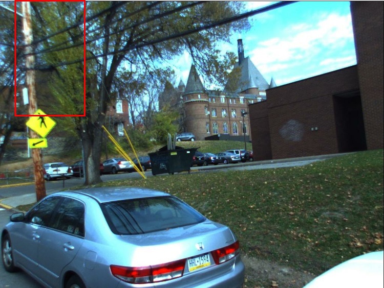
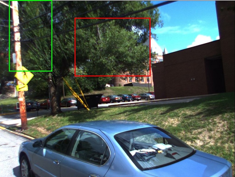
RGB

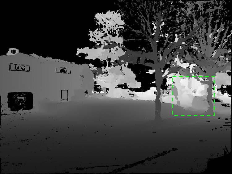
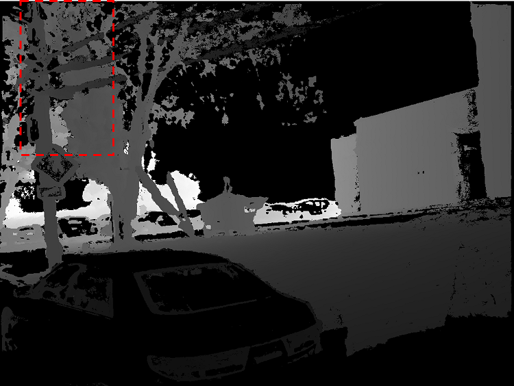
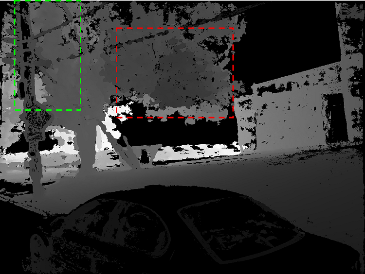
Ground Truth

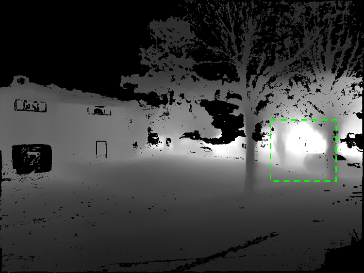
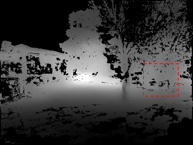
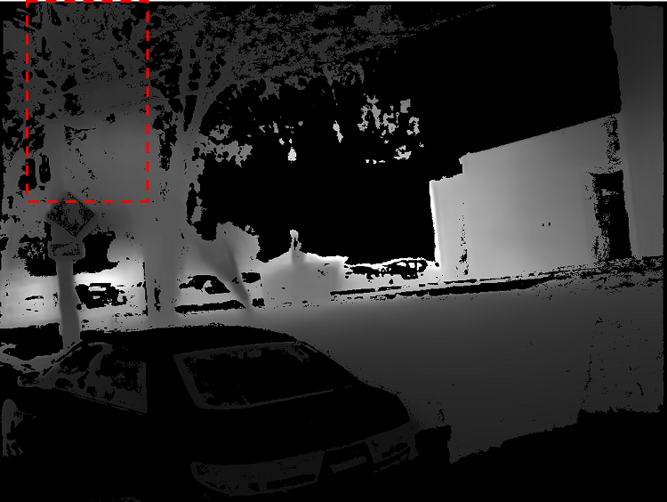
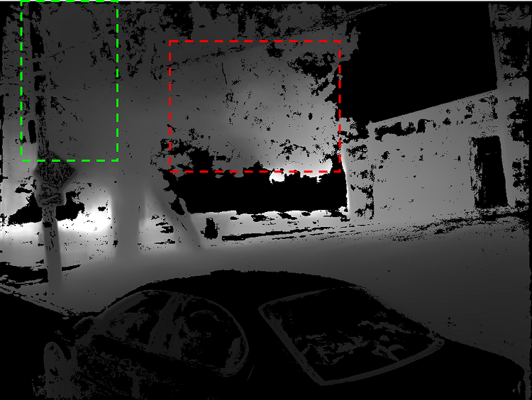
VNL [99]

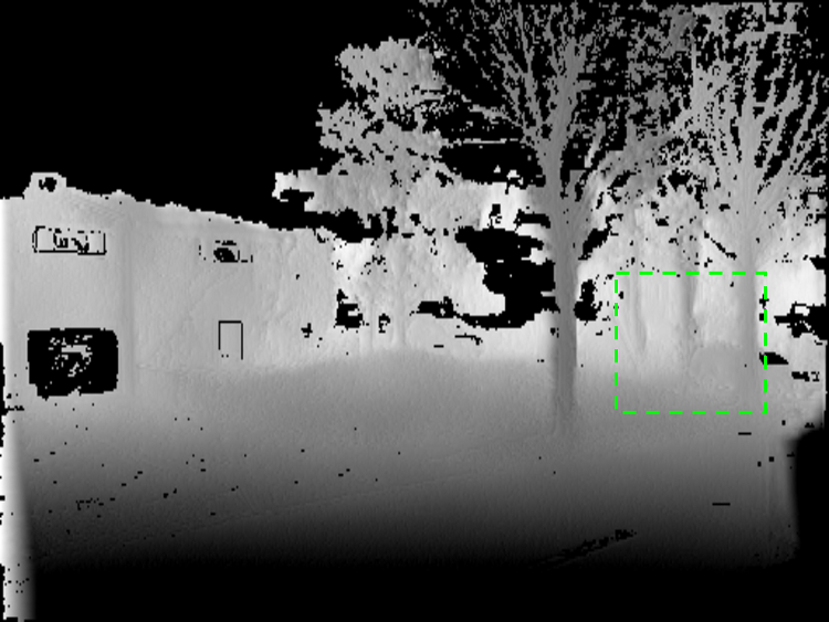
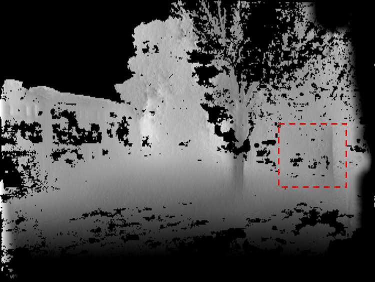
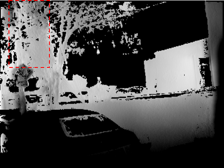
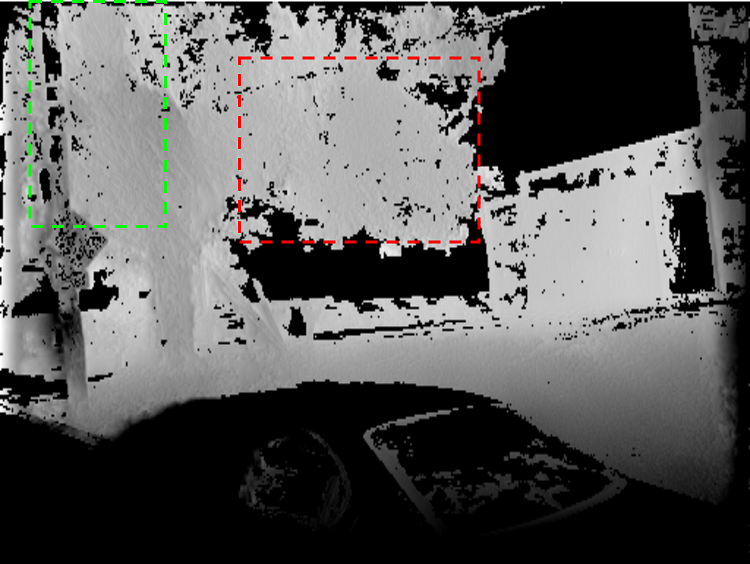
adareg [89]

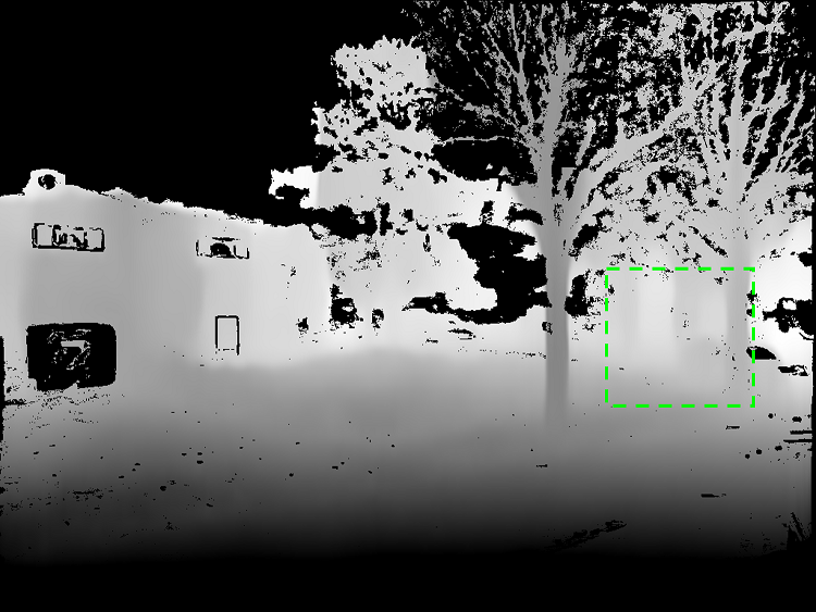
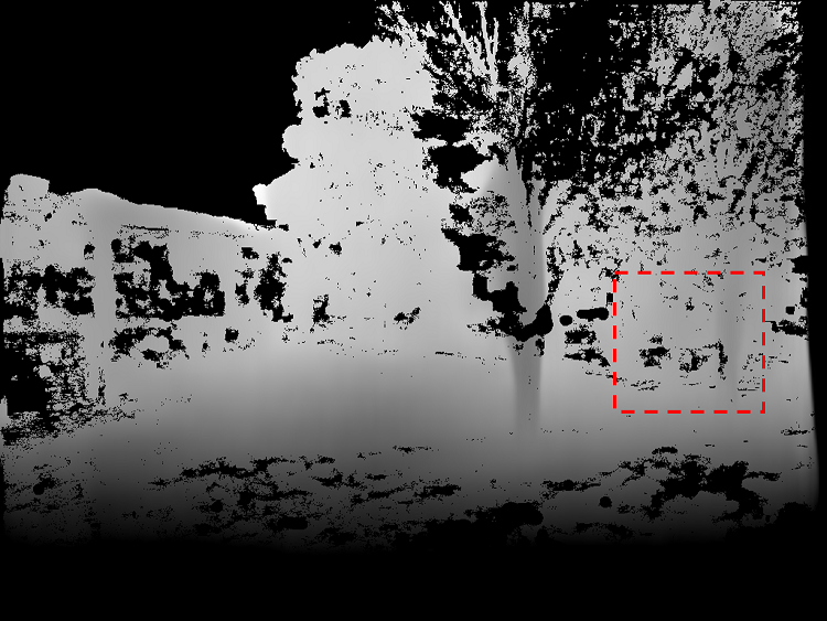
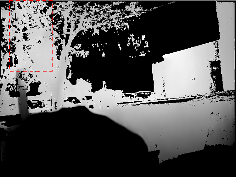
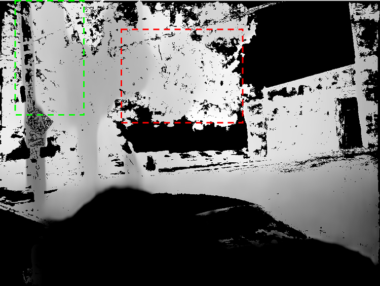
Monodepth2 [22]

Figure 7: Qualitative comparison results with illumination or vegetation changes. The conditions from top to down are C+MF, Nov. $22^{nd}$, LS+MF, Nov. $3^{rd}$, C+MF, Nov. $22^{nd}$ and C+F, Oct. $1^{st}$. Green blocks indicate good performance while red blocks are for bad results.

Then we investigate the fine-tuned models from KITTI to SeasonDepth and compare it with generalization without fine-tuning in Tab. 4. It can be seen that although most metrics are improved through fine-tuning, the improvement is still limited compared to other zero-shot evaluation results in Tab. 3, indicating that solely increasing the variability of training data cannot address the challenge of environmental changes. Qualitative results for different types of baselines are shown in Fig. 5. It can be seen that supervised methods BTS [47] and VNL [99] suffer from overfitting through the predicted pattern where the top and bottom areas are dark while the central areas are light, even for buildings.

Table 5: Cross-dataset performance on KITTI [84] with models fine-tuned on SeasonDepth and Cityscapes [14].

Method	MAE $\downarrow$	absErrorRel $\downarrow$	iMAE $\downarrow$	iRMSE $\downarrow$	sqErrorRel $\downarrow$
BTS [47] tuned on Cityscapes [14]	4.21±0.411	0.29±0.030	0.032±0.003	0.048±0.005	0.20±0.051
BTS [47] tuned on SeasonDepth (ous)	5.36±0.200	0.32±0.019	0.030±0.004	0.037±0.005	0.19±0.022
SfMLearner [110] tuned on Cityscapes [14]	6.40±0.202	0.42±0.019	0.045±0.003	0.060±0.004	0.38±0.05
SfMLearner [110] tuned on SeasonDepth (ous)	6.31±0.270	0.38±0.023	0.032±0.003	0.041±0.003	0.30±0.0338

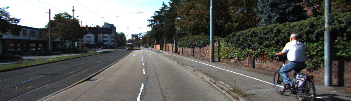
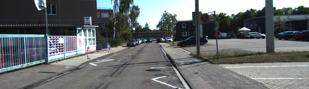
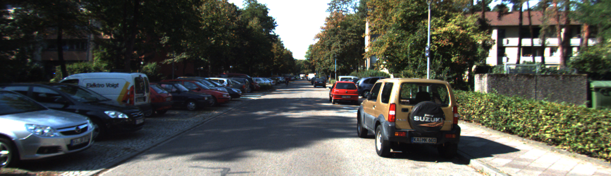
RGB

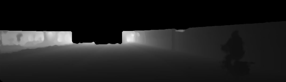
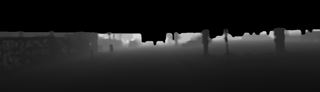
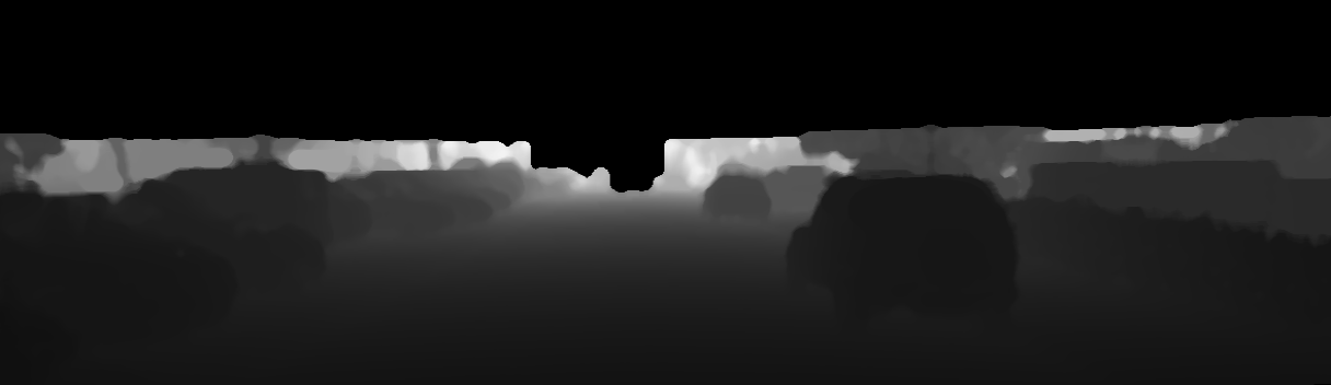
Ground Truth

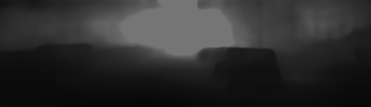
BTS [47] fine-tuned
on Cityscapes [14]

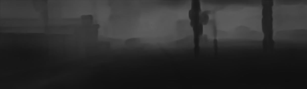
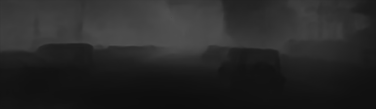
BTS [47] fine-tuned
on SeasonDepth

SfMLearner [110] fine-tuned on Cityscapes [14]

SfMLearner [110] fine-tuned on SeasonDepth

Figure 8: Qualitative comparison on KITTI [84] with depth prediction models fine-tuned on SeasonDepth and Cityscapes [14]

5.3 Influence of Challenging Environments

In this section, we further investigate which environment is more difficult to the current depth prediction models. The abbreviations of environments in Fig. 6 are S for Sunny, C for Cloudy, O for Overcast, LS for Low Sun, Sn for Snow, F for Foliage, NF for No Foliage, and MF for Mixed Foliage. From Fig. 6, we can see that dusk scenes in LS+MF, Nov. $3^{rd}$ and snowy scenes in LS+NF+Sn, Dec. $21^{st}$ pose great challenge for most algorithms, which points out directions for future research and safe applications. Besides, the consistent error bar in Fig. 6 shows such adverse environments always result in large deviations for all algorithms.

Under these adverse environmental conditions, promising algorithms can also be found. For the dusk or snowy scenes, some domain adaptation methods [2, 105] present impressive robustness under adverse scenes due to the various appearances of synthetic images. For the snowy scenes, self-supervised models are less influenced compared to supervised methods. Qualitative experimental results in Fig. 7 show how extreme illumination or vegetation changes affect depth prediction. From the top two rows, it can be seen that the illumination change of low sun makes the depth prediction of tree trunks less clear under the same vegetation condition as green and red blocks show. Also, no foliage tends to make telephone poles and tree trunks less distinguishable by comparing red and green blocks from the last two rows, while the depth prediction of heavy vegetation is difficult as red blocks show on the fourth row given the same illumination and weather condition. More results can be found in Appendix Sec. B.2.

5.4 Cross-dataset Comparison with Cityscapes

From the quantitative results in Tab. 5, the KITTI performance from models fine-tuned on SeasonDepth is mostly better than models fine-tuned on Cityscapes with similar fluctuation of model performance. Based on the qualitative performance in Fig. 8, we can find that models fine-tuned on SeasonDepth perform better than those fine-tuned on Cityscapes on the unseen KITTI dataset. Consequently, although the depth maps of SeasonDepth are reconstructed from structure from motion and do not contain dynamic objects, the ground truth accuracy is eligible to be used for model training compared to the stereo depth dataset Cityscapes, justifying our ground truth accuracy is adequate to be beneficial to cross-dataset generalization ability.

5.5 Further Discussion

In this section, we will discuss how to improve the robustness across multiple environments to boost more research on long-term robust visual perception. The key problem of long-term robust perception is the real-world out-of-distribution robustness of machine learning models [30], where images from changing environments act as samples from different distribution with respect to the training distribution. Since real-world environments are very hard to quantify using specific distribution distance, the robust perception is very challenging. Empirically, research about long-term performance under changing environments stems from visual place recognition and localization. Most of deep learning based methods leverage environmentally-insensitive perceptual auxiliary information like semantic [94, 4, 32], geometric [61, 62],or learn the domain-invariant representation [33, 107, 82] or image translation [34, 106] in multi-domain setting to deal with changing environments. Viewing the monocular depth prediction as pixel-level regression, we believe SeasonDepth will facilitate future research theoretically and empirically.

6 Conclusion

In this paper, a new dataset SeasonDepth is built for monocular depth prediction under different environments, and supervised and self-supervised state-of-the-art open-source algorithms are evaluated. From the experimental results, we find that there is still a long way to go to achieve robustness for long-term depth prediction and several promising avenues are given, pointing out self-supervised methods are more robust to changing environments. Through studying how adverse environments influence, our findings via this dataset and benchmark will impact the research on long-term robust perception and related applications.

Appendix A Building SeasonDepth Dataset

In this section, we present more details about the process of building SeasonDepth dataset and statistical analysis of depth maps in each environment.

A.1 Details in Building Dataset

We adopt the categorized slices of the Urban part according to [70] as original images after rectification through the camera intrinsic file. Specifically, we use slice2, slice3, slice7, slice8 as the split validation slices for cross-dataset evaluation and benchmark, slices slice4, slice5, slice6 are intended to treat as training sets, and slice9 is used as the test set for the evaluation of well-tuned methods. Note that since not all images from the original dataset are appropriate for depth prediction due to huge noise, e.g., a moving truck covering almost all the pixels, we remove such images in the final version. The numbers of images under all the environments for all slices in training, validation, and test set are shown in Tab. 6. The abbreviations of environments are S for Sunny, C for Cloudy, O for Overcast, LS for Low Sun, Sn for Snow, F for Foliage, NF for No Foliage, and MF for Mixed Foliage. It could be seen that the total number of validation set is larger than that of the training set with more different slices, which helps to make the benchmark results more accurate and reliable. Also, the training set can be used to fine-tune pre-trained models, which do not need too many images. Images from the left and right cameras are merged together in the same slice for calculation.

Table 6: Numbers of Images under All the Environments for All Slices

Environments	Training Set				Validation Set					Test Set
	slice4	slice5	slice6	All Slices	slice2	slice3	slice7	slice8	All Slices	slice9
S+NF Apr. 4th	221	129	543	893	382	450	190	449	1471	380
S+F Sept. 1st	116	230	190	536	385	464	249	490	1588	334
S+F Sept. 15th	202	213	526	941	335	329	462	457	1583	283
C+F Oct. 1st	406	205	626	1237	347	438	350	244	1379	338
S+F Oct. 19th	288	192	558	1038	301	439	412	230	1382	166
O+MF Oct. 28th	394	194	536	1124	333	418	362	442	1555	338
LS+MF Nov. 3rd	445	198	399	1042	335	447	203	416	1401	351
LS+MF Nov. 12th	0	221	552	762	352	500	357	501	1710	366
C+MF Nov. 22nd	323	163	578	1064	298	436	380	423	1537	321
LS+NF+Sn Dec. 21st	241	14	592	847	284	512	56	147	999	346
LS+F Mar. 4th	175	19	498	692	354	222	0	512	1088	382
O+F Jul. 28th	458	212	560	1230	256	425	384	467	1532	309
All Environments	3269	1980	6158	11407	3962	5080	3405	4778	17225	3944

We adopt COLMAP’s MVS pipeline [74, 75] to find the 3D structure and depth map. We follow the instruction on https://colmap.github.io/ with sequential SIFT matching with RANSAC, sparse reconstruction, and dense reconstruction. Some important detailed hyperparameters can be found in Tab. 7, while others are with the default configuration. To make full use of the image sequences, we adjust the sequential matching overlap to be 15 instead of the whole sequence, improving the local optimization with less noise. During each iteration of RANSAC algorithm in triangulation, the minimum inlier ratio for SIFT matching is set to be 0.65 for the consideration that most pixels of a single image are static in most cases. The maximum SIFT matching distance is 0.55 to adapt the distance of dynamic objects and improve efficiency. The image samples after SfM can be found in Fig. 9-(b)

The valid pixels of the original depth map are between the lower threshold and upper threshold to filter most noise pixels. For one thing, since the fields, forests, and cloud in the far distance away from the camera matter little to the depth prediction applications for autonomous driving, we truncate the depth values over 92% (80% in some cases) of the whole image to focus more on the near roads, vehicles, buildings, vegetation, etc. For another, due to the camera placement on both sides of the car, the very near descriptors of the road cannot be correctly matched during SfM and reconstructed for a dense depth map, which should be removed by filtering the pixel values less than 5% of the whole depth map. Besides, in the special cases where all the near-road noises appear on the bottom of the images, we directly filter the pixels with depth values greater than a threshold in that rectangular bottom area of the images. The samples after depth range truncation can be seen in Fig. 9-(c).

Although depth range truncation removes some pixels with too large depth values, there are still misrecontructed pixels of sky, cloud or shadow with normal depth values. We use PowerToys from https://github.com/microsoft/PowerToys to pick up typical HSV values for further refinement and denoising. As Tab. 8 shows, the minimal and maximal HSV values are given for some typical noises, including sky, cloud, reflections and shadows. For the clear or cloudy sky, Value tends to be high around 200 and Hue is usually blue or white. However, for those areas in the shadow of low sun, Saturation and Value are extremely low to be about 10% so the depth map pixels are too hard to be correctly reconstructed, which need to be filtered. The samples after HSV refinement are shown in Fig. 9-(d).

Though RANSAC algorithm inside the SfM and MVS pipeline largely removes pixels of the dynamic objects to ensure the accuracy of overall depth values, the dynamic pixels cannot be fully eliminated and the contours of objects are not clear as well. Therefore, we employ MaskRCNN [28] with pre-trained models from Detectron2 on https://github.com/facebookresearch/detectron2. We adopt the pre-trained model with configuration file of COCO-InstanceSegmentation/mask_rcnn_R50_FPN_3x.yaml and modify the MODEL.ROI_HEADS.SCORE_THRESH_TEST to be 0.5 to find the instance segmentation with the class of car, person and bus. To process the image directly, we modify the visualization part in the official colab notebook, omitting boxes, keypoints and labels and letting $\alpha=1$ in draw_polygon function to set the pixels of the target objects to be black. But semantic or instance segmentation cannot distinguish dynamic objects that need to be removed, we use human annotation to check whether segmented vehicles or pedestrians are moving or not, relabeling the missing dynamic objects and correcting the mislabeled objects. The depth map samples after all the post-processing can be found in Fig. 9-(e). Note that since there are often more mis-reconstructed depth pixels around thin objects like branches and poles, we manually filter some of them in the processing for accuracy and reliable evaluation.

Table 7: Some Important Hyperparameters for COLMAP

Process	Hyperparameter	Value
Sequential SIFT Matching	min_inlier_ratio	0.65
	max_distance	0.55
	min_num_inliers	50
	overlap_num	15
RANSAC	dyn_num_trials_multiplier	3.0
	confidence	0.99
	min_inlier_ratio	0.1
Sparse Reconstucion	abs_pose_min_inlier_ratio	0.25
	filter_max_reproj_error	4.0
	filter_min_tri_angle	1.5
Dense Reconstucion	geom_consistency_max_cost	3.0
	geom_consistency_regularizer	0.3

Table 8: Some Typical Noises and HSV Thresholds

Noise Source and Type	minimal threshold (H, S, V)	maximal threshold (H, S, V)
Blue Sky	(172, 5%, 40%)	(240, 90%, 100%)
White Cloud and Bright Reflections from Windows	(0, 0%, 100%)	(360, 100%, 100%)
Dark and Black Shadows	(0,0%,0%)	(0,0%,0)%
Dusk Cloud and Refections from Roads and Cars	(0,0%,70%)	(90,20%,100%)
Dusk Sky	(140, 11%, 40%)	(160, 50%, 100%)

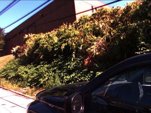
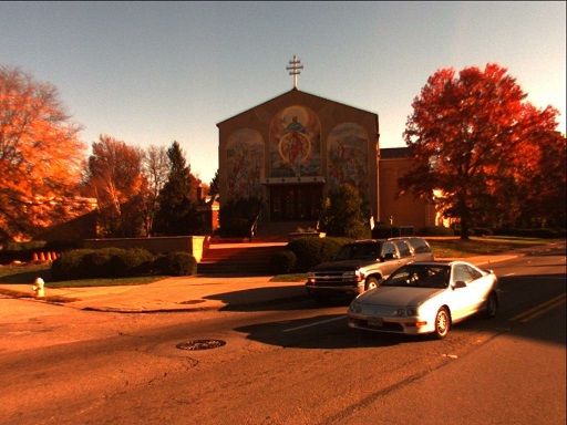
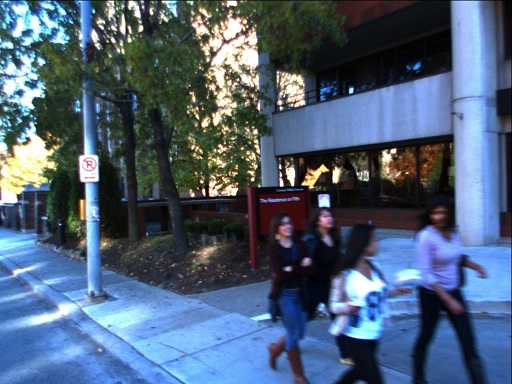
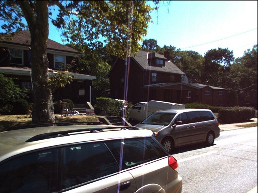
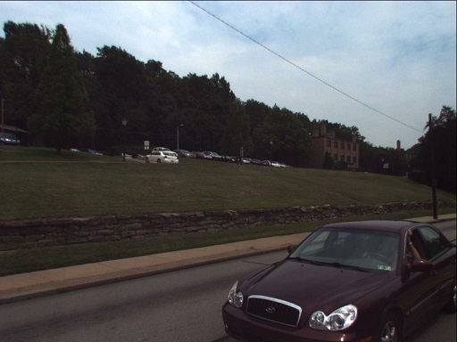
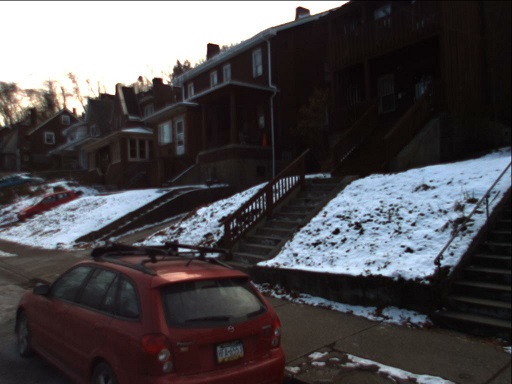
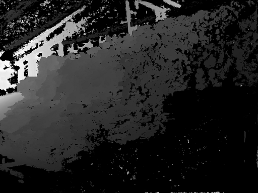
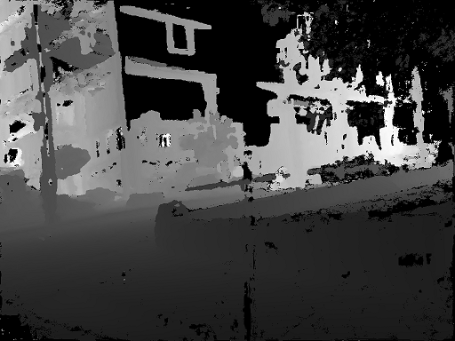
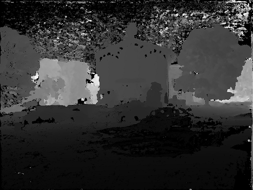
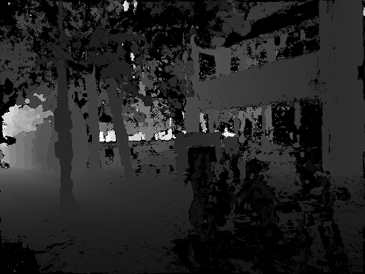
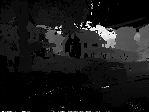
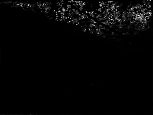
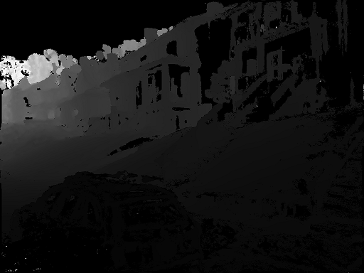
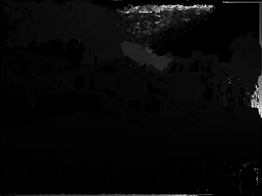
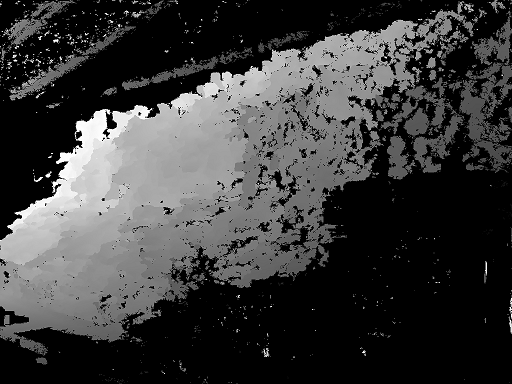
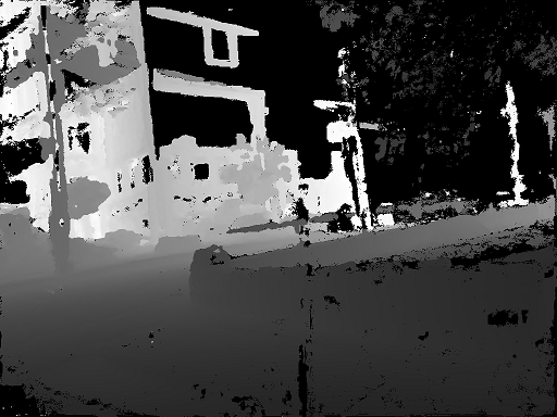
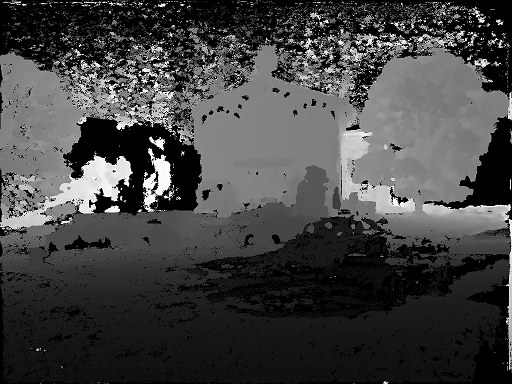
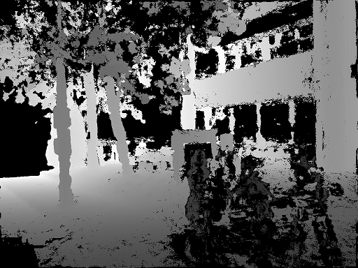
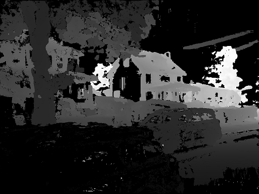
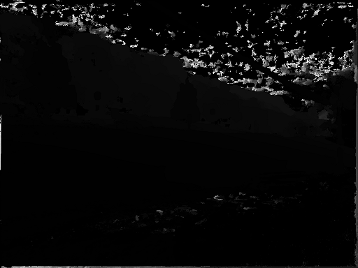
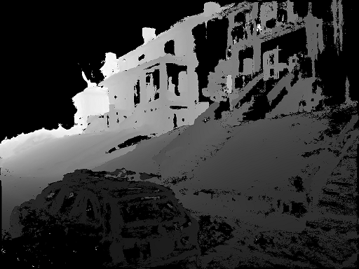
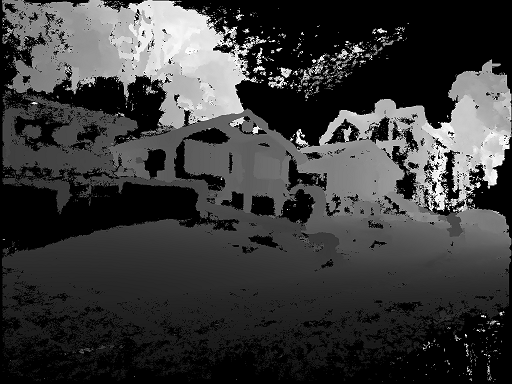
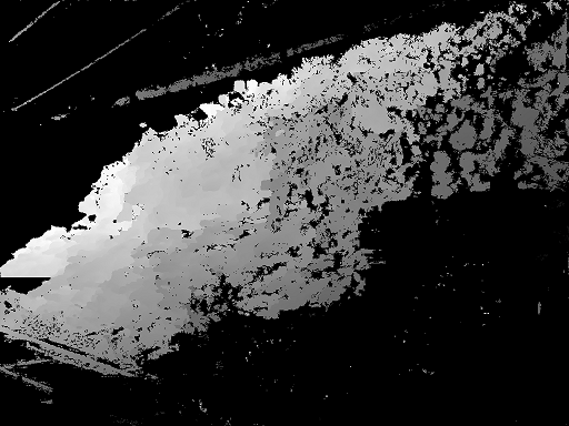
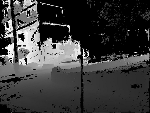
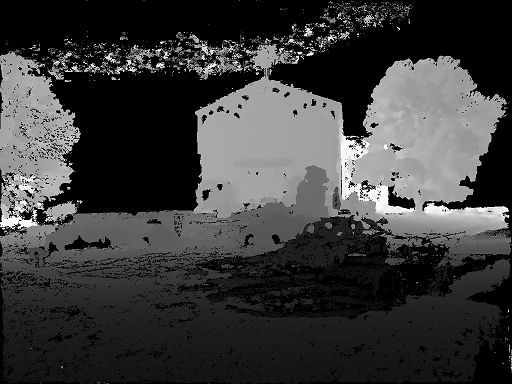
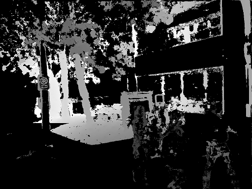
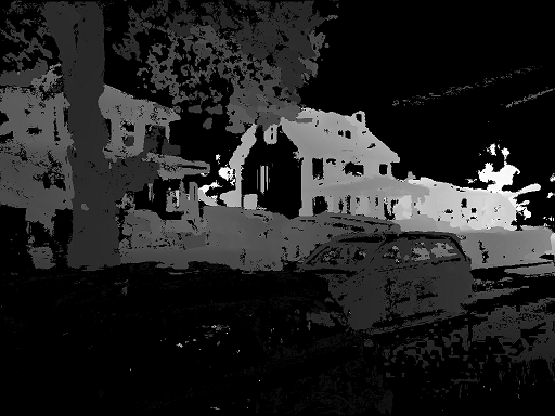
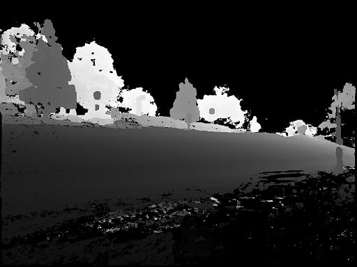
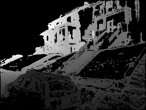
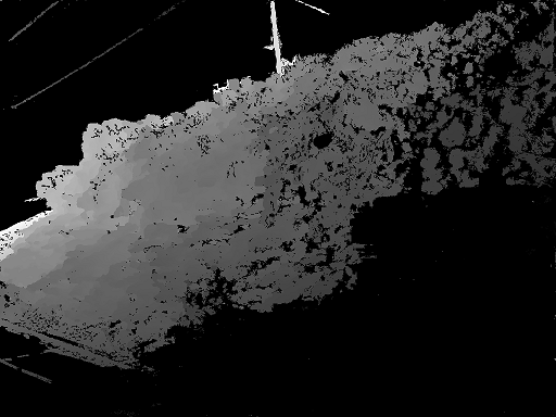
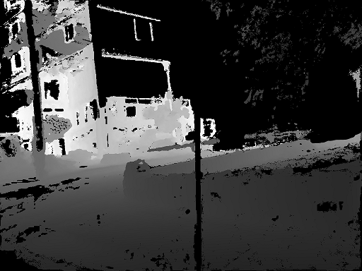
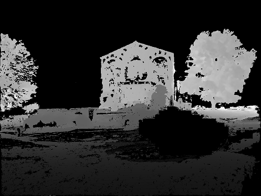
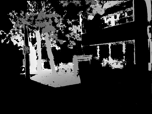
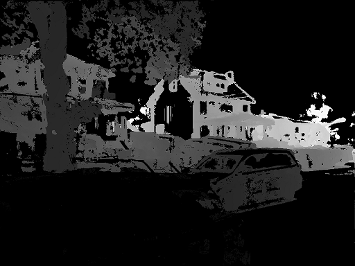
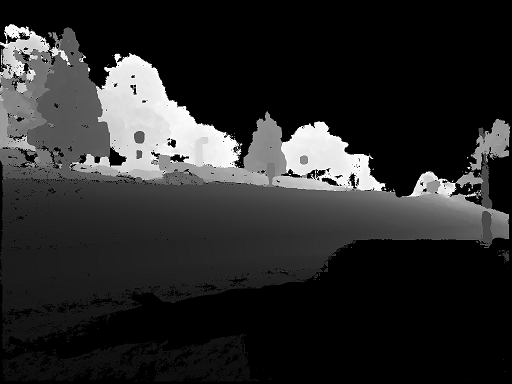
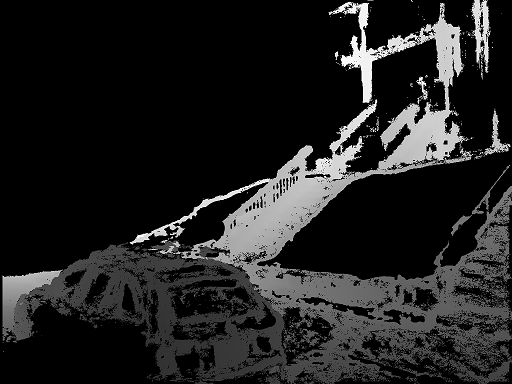
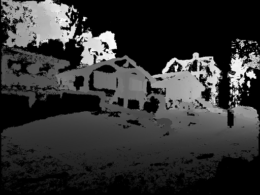
Figure 9: The processing samples given RGB image followed by normalized depth maps for clear visualization of (a) dense reconstruction, (b) range filtering, (c) HSV-based refinement and (d) manual post-processing.

A.2 Statistics and Analysis of Depth Map for Each Environment

Here we give the statistical analysis of the proposed SeasonDepth dataset for each environment. Since all the depth values are scale-free and not absolute for distance, it is not applicable to directly find the pixel value distribution for the dataset as [25, 85] do. However, the depth values of sequential frames in similar urban scenes under the same environment are similarly distributed, i.e. the depth values of images along similar streets and blocks are consistent. Then the key point is to align the distribution of each environment to the mean of all environments, obtaining the normalized whole distribution map and dismissing the scale discrepancy.

Therefore, we first find the original depth value distribution $p_{D_{i}}(x)$ for all the slices under each environment $i$. Then lower quartile $Q_{1}$ (25%), median $Q_{2}$ (50%) and upper quartile $Q_{3}$ (75%) are calculated for the original distribution of every environment and the mean value of quartiles can be found as reference quartiles$Q_{{1_{ref}}},Q_{{2_{ref}}},Q_{{3_{ref}}}$ for all $n$ environments,

$${Q_{{1_{ref}}}}=\frac{1}{n}\sum\limits_{i=1}^{n}{{Q_{{1_{i}}}}},{Q_{{2_{ref}}}}=\frac{1}{n}\sum\limits_{i=1}^{n}{{Q_{{2_{i}}}}},{Q_{{3_{ref}}}}=\frac{1}{n}\sum\limits_{i=1}^{n}{{Q_{{3_{i}}}}}$$

To find the scale normalization ratio $r_{i}$, we use arithmetic mean to measure the ratio of reference quartiles $Q_{{1_{ref}}},Q_{{2_{ref}}},Q_{{3_{ref}}}$ and other quartiles $Q_{{1_{i}}},Q_{{2_{i}}},Q_{{3_{i}}}$,

$$r_{i}=\frac{1}{3}(\frac{{{Q_{{1_{ref}}}}}}{{{Q_{{1_{i}}}}}}+\frac{{{Q_{{2_{ref}}}}}}{{{Q_{{2_{i}}}}}}+\frac{{{Q_{{3_{ref}}}}}}{{{Q_{{3_{i}}}}}})$$ (1)

Then the distribution $p_{D_{i}}(x)$ can be normalized to mean reference environment to obtain $p_{D\_norm_{i}}(x)$,

$$p_{D\_norm_{i}}(x)=r_{i}p_{D_{i}}(x)$$ (2)

After that, the normalized distribution of all the environments can be added directly to get the whole distribution. The distribution map of each environment can be found in Fig. 10. It can be seen that all the pixels follow a similar long-tail distribution, and the average y-axis numbers of per-image pixels overcome the bias caused by unbalanced image quantities across different environments. The normalization makes each distribution aligned on the x-axis, which can be directly added to obtain the total distribution map, as Fig. 3 shows.

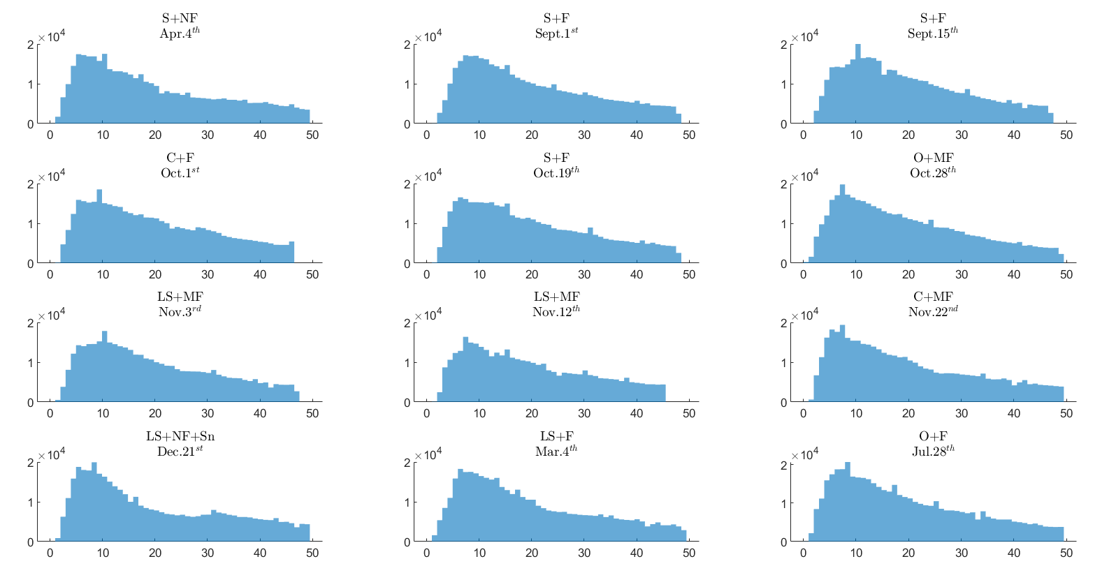
Figure 10: The normalized depth map distribution under all environments. The values of y-axes are the number of pixels with the value of abscissa on each image on average.

Appendix B SeasonDepth Benchmark

B.1 Details about Evaluated Models

For fairness in evaluating the performance algorithms under changing environments, we present the SeasonDepth benchmark with the well-tuned models on our training data and with no limit to the pretrained state-of-the-art models for the best results. Since there are only monocular videos with depth maps in our dataset, we report the results of some supervised learning methods and monocular video based self-supervised learning methods and leave other categories in the cross-dataset generalization benchmark. Specifically, the following supervised learning models are evaluated, DepthFormer [49] with implementation of https://github.com/zhyever/Monocular-Depth-Estimation-Toolbox/tree/main/configs/depthformer, BTS [47] with the implementation of https://github.com/cleinc/bts and DPT [65] with pretrained models on https://github.com/intel-isl/DPT/releases/download/1_0/dpt_hybrid-midas-501f0c75.pt from https://github.com/isl-org/DPT after fine-tuning over 60 epochs with our training set.

For the well-tuned self-supervised models on SeasonDepth benchmakr, we evaluate SUB-Depth [108] with ResNet18 as the backbone for 5 epochs using learning rate 0.0001, VADepth [92] from https://github.com/xjixzz/vadepth-net, Monodepth2 [22] from https://github.com/nianticlabs/monodepth2, SfMLearner [110] from https://github.com/ClementPinard/SfmLearner-Pytorch and ManyDepth [88] from https://github.com/nianticlabs/manydepth as baselines.

For the cross-dataset evaluation for the generalization of depth prediction, we further benchmark the representative supervised, self-supervised, and domain adaptation models from the well-known KITTI leaderboard [84], which are with open-source codes and pre-trained models for a fair comparison. Here are some important details for all the evaluated baselines. Our experiments are conducted on two NVIDIA 2080Ti cards with 64G RAM on Ubuntu 18.04 system. The evaluation metrics are modified based on development kit [84] on http://www.cvlibs.net/datasets/kitti/eval_depth.php?benchmark=depth_prediction.

For the supervised methods, we evaluate four representative methods, Eigen et al. [17], BTS [47], MegaDepth [50] VNL [99]. Eigen et al. propose the first CNNs-based depth prediction method and introduce the famous Eigen split of KITTI dataset for depth prediction benchmark. We hence evaluate this representative method using the PyTorch implementation through https://github.com/DhruvJawalkar/Depth-Map-Prediction-from-a-Single-Image-using-a-Multi-Scale-Deep-Network with the improved image gradient component in the newer loss to see the performance across multiple environments. Supervised work BTS ranks $4th$ on the KITTI benchmark and we test it on https://github.com/cogaplex-bts/bts using the pre-trained model DenseNet161 on Eigen split. We further fine-tune this pre-trained model of BTS on our training set for 20 epochs with a batch size of 16. The best performance of $Average$ metric is obtained from epoch 20. Due to the scaleless and partially validated ground truth, we only calculate the non-zero pixels and conduct alignment using the mean value for loss when fine-tuning. Note that focal value does not influence the experimental results due to the relative scale of the depth metrics. We test the MegaDepth method according to https://www.cs.cornell.edu/projects/megadepth/ with the MegaDepth pre-trained models as described in the paper and all the hyperparameters are set as default. VNL is evaluated using https://github.com/YvanYin/VNL_Monocular_Depth_Prediction with the pre-trained model of ResNext101_32x4d backbone and trained on KITTI dataset.

Table 9: $AbsRel$ Results (Lower Better) under Each Environment: Mean(Standard Deviation)

Method	S+NF Apr. 4th	S+F Sept. 1st	S+F Sept. 15th	C+F Oct. 1st	S+F Oct. 19th	O+MF Oct. 28th	LS+MF Nov. 3rd	LS+MF Nov. 12th	C+MF Nov. 22nd	LS+NF+Sn Dec. 21st	LS+F Mar. 4th	O+F Jul. 28th
Eigen et al. [17]	1.080(0.39)	1.111(0.40)	1.034(0.43)	1.061(0.40)	1.043(0.40)	1.072(0.38)	1.233(0.43)	1.125(0.37)	1.008(0.32)	1.067(0.42)	1.136(0.54)	1.150(0.55)
BTS [47]	0.697(0.29)	0.652(0.24)	0.605(0.24)	0.641(0.29)	0.647(0.27)	0.646(0.28)	0.758(0.35)	0.574(0.27)	0.637(0.27)	0.848(0.36)	0.761(0.38)	0.657(0.28)
MegaDepth [50]	0.514(0.20)	0.494(0.16)	0.471(0.17)	0.494(0.18)	0.486(0.18)	0.510(0.18)	0.574(0.21)	0.512(0.18)	0.489(0.19)	0.553(0.26)	0.547(0.25)	0.530(0.24)
VNL [99]	0.321(0.16)	0.294(0.13)	0.257(0.11)	0.281(0.14)	0.281(0.13)	0.302(0.16)	0.357(0.20)	0.271(0.14)	0.282(0.14)	0.380(0.21)	0.342(0.21)	0.306(0.15)
Monodepth [23]	0.450(0.19)	0.437(0.16)	0.389(0.14)	0.424(0.18)	0.434(0.18)	0.432(0.16)	0.475(0.20)	0.418(0.17)	0.421(0.16)	0.465(0.21)	0.441(0.20)	0.449(0.20)
adareg [89]	0.553(0.22)	0.515(0.16)	0.473(0.18)	0.489(0.20)	0.509(0.19)	0.493(0.19)	0.515(0.17)	0.463(0.18)	0.498(0.20)	0.523(0.20)	0.543(0.29)	0.515(0.25)
monoResMatch [83]	0.536(0.31)	0.466(0.24)	0.398(0.19)	0.444(0.27)	0.463(0.25)	0.479(0.31)	0.526(0.28)	0.428(0.25)	0.486(0.28)	0.600(0.40)	0.544(0.39)	0.475(0.26)
SfMLearner [110]	0.745(0.29)	0.682(0.26)	0.644(0.27)	0.657(0.28)	0.684(0.29)	0.671(0.28)	0.718(0.35)	0.627(0.27)	0.698(0.27)	0.765(0.32)	0.714(0.29)	0.713(0.31)
PackNet [25]	0.715(0.27)	0.740(0.23)	0.680(0.26)	0.692(0.26)	0.672(0.24)	0.728(0.27)	0.806(0.27)	0.732(0.22)	0.682(0.25)	0.684(0.22)	0.727(0.36)	0.803(0.43)
Monodepth2 [22]	0.476(0.18)	0.414(0.15)	0.383(0.17)	0.412(0.17)	0.396(0.17)	0.412(0.17)	0.441(0.23)	0.380(0.16)	0.414(0.16)	0.452(0.20)	0.459(0.20)	0.402(0.16)
CC [67]	0.613(0.23)	0.633(0.23)	0.587(0.25)	0.640(0.24)	0.627(0.27)	0.652(0.24)	0.768(0.25)	0.649(0.23)	0.593(0.24)	0.644(0.28)	0.673(0.34)	0.703(0.39)
SGDepth [40]	0.635(0.24)	0.650(0.21)	0.605(0.23)	0.640(0.23)	0.628(0.23)	0.649(0.24)	0.726(0.26)	0.659(0.20)	0.599(0.19)	0.651(0.23)	0.661(0.31)	0.671(0.29)
Atapour et al. [2]	0.741(0.27)	0.658(0.22)	0.619(0.24)	0.643(0.27)	0.667(0.27)	0.686(0.29)	0.658(0.28)	0.627(0.29)	0.708(0.27)	0.778(0.32)	0.728(0.29)	0.724(0.30)
T2Net [105]	0.809(0.39)	0.830(0.29)	0.732(0.34)	0.796(0.35)	0.760(0.33)	0.831(0.35)	0.968(0.33)	0.797(0.29)	0.776(0.33)	0.869(0.37)	0.912(0.48)	0.849(0.45)
GASDA [103]	0.443(0.24)	0.414(0.20)	0.402(0.21)	0.420(0.26)	0.426(0.24)	0.412(0.22)	0.495(0.26)	0.416(0.24)	0.429(0.24)	0.521(0.29)	0.460(0.26)	0.423(0.26)

Table 10: $a_{1}$ Results (Higher Better) under Each Environment: Mean(Standard Deviation)

Method	S+NF Apr. 4th	S+F Sept. 1st	S+F Sept. 15th	C+F Oct. 1st	S+F Oct. 19th	O+MF Oct. 28th	LS+MF Nov. 3rd	LS+MF Nov. 12th	C+MF Nov. 22nd	LS+NF+Sn Dec. 21st	LS+F Mar. 4th	O+F Jul. 28th
Eigen et al. [17]	0.336(0.14)	0.335(0.12)	0.337(0.14)	0.352(0.14)	0.348(0.13)	0.345(0.13)	0.311(0.12)	0.338(0.13)	0.360(0.12)	0.351(0.13)	0.341(0.13)	0.321(0.13)
BTS [47]	0.200(0.11)	0.201(0.10)	0.233(0.10)	0.218(0.11)	0.225(0.12)	0.217(0.12)	0.183(0.12)	0.263(0.15)	0.221(0.11)	0.161(0.10)	0.185(0.10)	0.201(0.11)
MegaDepth [50]	0.417(0.14)	0.430(0.13)	0.439(0.15)	0.422(0.16)	0.427(0.13)	0.420(0.15)	0.377(0.13)	0.408(0.15)	0.436(0.15)	0.399(0.17)	0.402(0.17)	0.421(0.15)
VNL [99]	0.513(0.21)	0.532(0.18)	0.579(0.18)	0.554(0.20)	0.550(0.19)	0.535(0.20)	0.463(0.20)	0.579(0.19)	0.557(0.21)	0.442(0.19)	0.499(0.23)	0.528(0.21)
Monodepth [23]	0.456(0.17)	0.446(0.15)	0.485(0.13)	0.463(0.15)	0.453(0.14)	0.460(0.15)	0.434(0.14)	0.463(0.14)	0.463(0.14)	0.428(0.17)	0.464(0.16)	0.445(0.15)
adareg [89]	0.363(0.18)	0.387(0.14)	0.419(0.15)	0.422(0.17)	0.389(0.14)	0.417(0.15)	0.389(0.15)	0.444(0.16)	0.405(0.17)	0.393(0.15)	0.398(0.16)	0.431(0.18)
monoResMatch [83]	0.363(0.21)	0.386(0.18)	0.439(0.18)	0.428(0.20)	0.391(0.17)	0.400(0.19)	0.354(0.18)	0.429(0.20)	0.385(0.19)	0.342(0.19)	0.368(0.20)	0.386(0.17)
SfMLearner [110]	0.251(0.10)	0.268(0.09)	0.270(0.09)	0.284(0.11)	0.268(0.11)	0.271(0.10)	0.271(0.11)	0.292(0.12)	0.258(0.09)	0.245(0.09)	0.253(0.09)	0.254(0.09)
PackNet [25]	0.436(0.13)	0.394(0.13)	0.422(0.15)	0.435(0.15)	0.430(0.14)	0.429(0.14)	0.368(0.13)	0.403(0.12)	0.458(0.13)	0.450(0.13)	0.444(0.14)	0.386(0.17)
Monodepth2 [22]	0.366(0.17)	0.423(0.16)	0.465(0.19)	0.438(0.17)	0.454(0.18)	0.442(0.16)	0.418(0.19)	0.473(0.18)	0.426(0.17)	0.403(0.17)	0.391(0.18)	0.452(0.16)
CC [67]	0.493(0.19)	0.478(0.18)	0.501(0.21)	0.480(0.20)	0.494(0.19)	0.479(0.19)	0.400(0.15)	0.480(0.18)	0.525(0.18)	0.488(0.19)	0.483(0.20)	0.445(0.21)
SGDepth [40]	0.497(0.17)	0.459(0.16)	0.487(0.19)	0.475(0.18)	0.487(0.17)	0.487(0.18)	0.437(0.14)	0.475(0.15)	0.525(0.15)	0.483(0.16)	0.495(0.18)	0.449(0.19)
Atapour et al. [2]	0.281(0.12)	0.304(0.12)	0.313(0.12)	0.320(0.13)	0.309(0.13)	0.301(0.11)	0.309(0.13)	0.325(0.15)	0.287(0.11)	0.287(0.11)	0.282(0.11)	0.284(0.12)
T2Net [105]	0.421(0.17)	0.367(0.15)	0.416(0.17)	0.403(0.17)	0.416(0.16)	0.390(0.16)	0.340(0.13)	0.404(0.15)	0.429(0.17)	0.349(0.14)	0.363(0.16)	0.393(0.17)
GASDA [103]	0.414(0.18)	0.418(0.16)	0.426(0.14)	0.429(0.17)	0.428(0.16)	0.427(0.15)	0.377(0.16)	0.433(0.18)	0.420(0.17)	0.347(0.19)	0.383(0.19)	0.427(0.16)

For self-supervised methods, we further categorize them and choose baselines respectively, i.e. Monodepth [23], adareg [89] and monoResMatch [83] for stereo geometry based methods, SfMLearner [110], Monodepth2 [22] and PackNet [25] for monocular video SfM based methods, and CC [67] and SGDepth [40] for multi-task learning with monocular SfM unsupervised pipeline. We also report the results of FSRE-Depth [37] CADepth-Net [98] VADepth [92] from recent work [92], which uses our validation set for the generalization evaluation from KITTI pretrained models. For stereo geometry based unsupervised methods, Monodepth method is evaluated using https://github.com/OniroAI/MonoDepth-PyTorch, which is able to reproduce similar results to those in the paper on Eigen split. We test the model of adareg from https://github.com/alexklwong/adareg-monodispnet pre-trained with Eigen split. monoResMatch is tested through https://github.com/fabiotosi92/monoResMatch-Tensorflow with KITTI pretrined model with default hyperparameters. For sequence SfM based unsupervised methods, we adopt https://github.com/ClementPinard/SfmLearner-Pytorch to benchmark SfMLearner for better performance than original repo with slight modification. We further fine-tune the pre-trained models of dispnet_model_best and exp_pose_model_best on our training set using default configuration file with sequence length of 5 for 20 epochs to get the best performance on $Average$ metric at epoch 20. We use the model of ResNet18 pre-trained on ImageNet and fine-tuned on KITTI with the resolution of $640\times 192$ to test PackNet on https://github.com/TRI-ML/packnet-sfm. Similarly, in order to incorporate stereo geometric constraint into the monocular SfM framework, we use the model of mono+stereo pre-trained on ImageNet and KITTI with the resolution of $640\times 192$ to evaluate the performance of Monodepth2 on https://github.com/nianticlabs/monodepth2. For the multi-task SfM unsupervised learning methods, CC is evaluated with DispNet, PoseNet, MaskNet and FlowNet pre-trained model on KITTI through https://github.com/anuragranj/cc. We also test another work SGDepth on https://github.com/ifnspaml/SGDepth with the full model of semantic segmentation and depth prediction with the resolution of $640\times 192$.

Since synthetic datasets like V-KITTI include multiple environments in spite of existing domain gap, we additionally evaluate the performance of three domain adaptation methods from KITTI benchmark, Atapour et al. [2], T2Net [105] and GASDA [103]. We follow the instruction on https://github.com/atapour/monocularDepth-Inference to evaluate the method proposed by Atapour et al. with the model pre-trained on KITTI and DeepGTAV [59]. T2Net is tested on https://github.com/lyndonzheng/Synthetic2Realistic with the weakly-supervised pre-trained model for outdoor scenes of KITTI and V-KITTI. We then evaluate the performance of GASDA on https://github.com/sshan-zhao/GASDA with the model pre-trained on V-KITTI and KITTI using self-supervised stereo geometric information.

B.2 Detailed Evaluation Results and Analysis

B.2.1 Cross-Dataset Performance under Different Environments

In this section, the detailed results with mean values and standard deviations across multiple environments are shown in Tab. 10 and Tab. 10, it can be seen that models with larger mean values tend to have more significant deviation for each environment. However, though there are some large standard deviations in Tab. 10 and Tab. 10, the quality of depth map ground truths is assured. So we attribute it to the poor generalization ability of those algorithms since not all the methods present such poor results with too large variances, which cannot be correctly analyzed.

Moreover, all the evaluated baselines are visualized after adjustment under typical challenging environments, including dark illumination, snowy scene, and complex vegetation. See Fig. 11 for more details. From the results of supervised methods, it can be seen that the patterns of predicted depth maps are similar, especially for BTS [47] and VNL [99], where the top and bottom areas are dark while the middle areas are bright due to overfitting, see buildings as examples. But VNL [99] shows the advantage in depth details (e.g. telephone poles and vegetation) in the middle areas which accounts for the best average performance.

Stereo training involved self-supervised methods (including Monodepth2 [22] and GASDA [103]) perform best continuous depth results for the same entity under all environments, e.g. depth values of buildings. Monocular video-based self-supervised methods do better in distinguishing relative depth from far and near areas, e.g. depth values for objects along different directions of roads, especially for multi-task learning ones CC [67] and SGDepth [40]. Besides, domain adaptation methods still suffer from domain gaps, which shows that synthetic multi-environment images help little to improve performance under real-world changing environments.

O+MF

Oct. 28th

LS+NF+Sn

Dec. 21st

S+F

Sept. 15th

S+NF

Apr. 4th

LS+MF

Nov. 3rd

LS+MF

Nov. 12th

To be continued

O+MF

Oct. 28th

LS+NF+Sn

Dec. 21st

S+F

Sept. 15th

S+NF

Apr. 4th

LS+MF

Nov. 3rd

LS+MF

Nov. 12th

Figure 11: Qualitative results for all the baselines with multiple illuminations, vegetation and weather conditions.

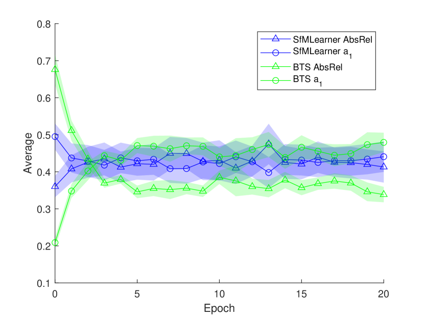
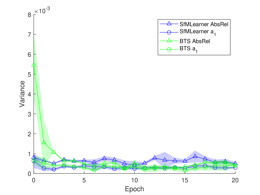
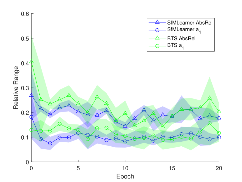
Figure 12: Performance evolution after fine-tuning on SeasonDepth training set from KITTI pretrained models.

B.2.2 Analysis of Performance of Fine-tuned Models

As the comparison of zero-shot cross-dataset evaluation from KITTI to SeasonDepth on the validation set, we use our training set to fine-tune one supervised [47] and one self-supervised model [110] from KITTI, which initially perform poor zero-shot results, to alleviate the impact of dataset bias between KITTI and SeasonDepth. Since our dataset does not contain stereo images, segmentation ground truth, and KITTI-like scenarios, just like in V-KITTI, the stereo training based, semantic segmentation involved multi-task training and domain adaptation models are omitted for the sake of fairness.

Besides results in Tab. 4, we present the evaluation results along training epochs with shadows of cross-slice standard deviation after zooming 0.5, 0.2, and 0.5 times in Fig. 12. It can be seen that after the fine-tuning, overall performance is improved while some $Variance$ and $RelativeRange$ results still perform badly, especially for SfMLearner [110], showing that the naive fine-tuning with more data will not help too much compared to other zero-shot evaluations in Tab. 3.

B.3 Cross-dataset Comparison with Cityscapes

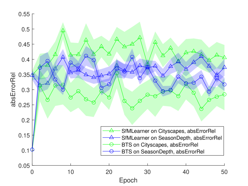
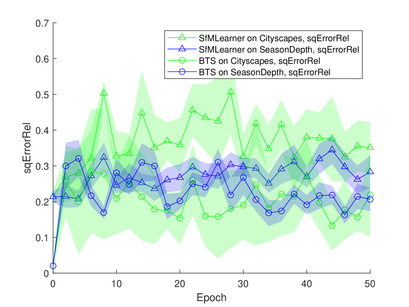
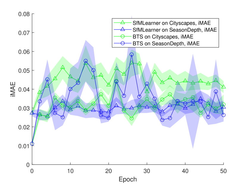
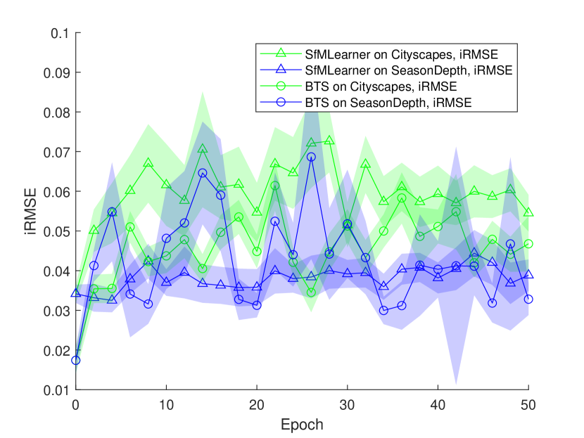
Figure 13: Cross-dataset performance evolution on KITTI validation set [84] with models fine-tuned on SeasonDepth and Cityscapes [14].

In this section, we present more details about the cross-dataset comparison experiment with Cityscapes to justify our depth quality for model training. As it is introduced in Sec. B.1, we choose the KITTI pre-trained models for BTS and SfMLearner methods, and fine-tune them on our training set and Cityscapes [14] for 50 epochs, respectively. Finally, we evaluate the cross-dataset transfer performance on the KITTI validation set [84] using development kit from http://www.cvlibs.net/datasets/kitti/eval_depth.php?benchmark=depth_prediction. We choose 11407 images from train_extra in Cityscapes [14] to fine-tune the models, which is exactly the same amount of images in our training set to make the comparison fair.

To fine-tune the self-supervised model of SfMLearner, we set batch_size to be 4, epoch_size to be 1000 and sequence_length to be 1000. Along with the instructions to train with own data https://github.com/ClementPinard/SfmLearner-Pytorch/issues/108, we crop a quarter of the bottom in the image and resize it to be $416\times 128$ to remove the car logo in Cityscapes dataset. We change the intrinsic parameters accordingly to make them consistent with cropped images. For a fair comparison, we also conduct such cropping for the images from the SeasonDepth dataset. When testing the KITTI validation set, we resize the images to $416\times 128$ before feeding them into the networks.

When fine-tuning the supervised BTS model, we set batch_size to be 16, input_size to be $256\times 192$ for SeasonDepth images and $256\times 128$ for Cityscapes images. For depth ground truth, we directly adopt the depth maps in Cityscapes as supervision signals while for the SeasonDepth dataset, we only consider the non-zero pixels and conduct alignment using mean value to the ground truth to construct loss when fine-tuning. The experimental results show that such alignment to construct supervised loss is effective using our dataset for supervised model training.

Besides the results in Tab. 5, we present the KITTI performance evolution over epochs with models fine-tuned on SeasonDepth and Cityscapes in Fig. 13. We can see that although the performance will be degraded compared to the KITTI pre-trained models due to domain shift when fine-tuning, the performance fine-tuned on SeasonDepth is better than models fine-tuned on Cityscapes, especially for SfMLearner method and $iMAE$ and $iRMSE$ metrics. Besides, the fluctuation of models fine-tuned on SeasonDepth is much less than those fine-tuned on Cityscapes in terms of $absErrorRel$ and $sqErrorRel$ metrics. Consequently, although the depth maps of SeasonDepth are reconstructed from structure from motion and do not contain dynamic objects, the ground truth accuracy is eligible to be used for model training compared to the stereo depth dataset Cityscapes, justifying our ground truth accuracy is adequate though it is not perfect.

Appendix C Limitation and Discussion

In this section, we discuss the limitation of our work. As mentioned before, our SeasonDepth dataset is built based on the CMU Visual Localization dataset, which was initially collected for visual localization and contained multiple scenes but without challenging night scenes. Although it is different from the dataset for autonomous driving like KITTI, which causes concern about the evaluation due to the domain gap. However, based on the experimental evidence, it is acceptable that fine-tuned models only provide limited help in terms of $Variance$ and $RelativeRange$. Although dynamic objects are not included in the dataset to ensure accuracy and reliability, it does not affect the evaluation for real driving applications because it cannot be distinguished whether the objects are dynamic or static given a single monocular image when testing. And the cross-dataset justification experiment also shows that missing dynamic objects do not influence the model training too much. Consequently, the evaluation of the depth prediction of static objects can reveal the performance of dynamic objects, although they are not involved in the ground truth.

Besides, though normalizing the scale of evaluation metrics through alignment of mean and variance can also be done through quantile alignment shown in Sec A.2, it is more sensitive to noise to adopt quantile-based alignment of every single image for evaluation. Although we try our best to survey and test the open-source representative models as much as possible, it is impossible to involve all the monocular depth prediction methods in our benchmark. So we release the training, validation and test set, and benchmark toolkit to make up for it. Another limitation is that it is not straightforward to train models on the dataset because of the ground truths of scaleless relative values, but it can be trained after the mean value alignment to the ground truth just as the fine-tuned BTS does. It can also reflect how environmental changes affect depth prediction models and give hints of what kind of method is more promising to this problem.

Appendix D Discussion on Societal Impacts

To our best knowledge, we are the first work focusing on changing environments on monocular depth prediction tasks, which has great significance to long-term or lifelong autonomous driving and outdoor mobile robotics. The robustness of the depth prediction algorithm is important to the safety of vehicles and pedestrians from the long-run perspective.

However, there are also some potential negative societal impacts. First, our dataset is not that general because the original dataset CMU Visual Localization dataset is only collected in one city, which may mislead the algorithm to overfit on similar scenes, leading to instability and risks when used in complex scenes for applications. Second, privacy is another problem. Although the dataset is secondarily derived and there are many licenses on it, malicious and unintended uses may still happen, e.g. collect the human faces or properties of the locals, which may violate the privacy right and cause other problems.

Dismissing such concerns needs the efforts of research, industry, and other social organizations. For example, researchers and engineers should thoroughly evaluate the performance and robustness of algorithms with environmental changes despite using our dataset to ensure the safety of autonomous driving. Social organizations should also keep an eye on such open-source real-world datasets to avoid illegal use.

References

- [1] Manuel López Antequera, Pau Gargallo, Markus Hofinger, Samuel Rota Bulò, Yubin Kuang, and Peter Kontschieder. Mapillary planet-scale depth dataset. In European Conference on Computer Vision, pages 589–604. Springer, 2020.
- [2] Amir Atapour-Abarghouei and Toby P Breckon. Real-time monocular depth estimation using synthetic data with domain adaptation via image style transfer. In Proceedings of the IEEE Conference on Computer Vision and Pattern Recognition, pages 2800–2810, 2018.
- [3] Hernán Badino, Daniel Huber, and Takeo Kanade. Visual topometric localization. In 2011 IEEE Intelligent Vehicles Symposium (IV), pages 794–799. IEEE, 2011.
- [4] Assia Benbihi, Matthieu Geist, and Cédric Pradalier. Image-based place recognition on bucolic environment across seasons from semantic edge description. 2020.
- [5] Shariq Farooq Bhat, Ibraheem Alhashim, and Peter Wonka. Adabins: Depth estimation using adaptive bins. In Proceedings of the IEEE/CVF Conference on Computer Vision and Pattern Recognition, pages 4009–4018, 2021.
- [6] Jiawang Bian, Zhichao Li, Naiyan Wang, Huangying Zhan, Chunhua Shen, Ming-Ming Cheng, and Ian Reid. Unsupervised scale-consistent depth and ego-motion learning from monocular video. Advances in neural information processing systems, 32, 2019.
- [7] Jia-Wang Bian, Huangying Zhan, Naiyan Wang, Zhichao Li, Le Zhang, Chunhua Shen, Ming-Ming Cheng, and Ian Reid. Unsupervised scale-consistent depth learning from video. International Journal of Computer Vision, 129(9):2548–2564, 2021.
- [8] Behzad Bozorgtabar, Mohammad Saeed Rad, Dwarikanath Mahapatra, and Jean-Philippe Thiran. Syndemo: Synergistic deep feature alignment for joint learning of depth and ego-motion. In Proceedings of the IEEE International Conference on Computer Vision, pages 4210–4219, 2019.
- [9] Vincent Casser, Soeren Pirk, Reza Mahjourian, and Anelia Angelova. Depth prediction without the sensors: Leveraging structure for unsupervised learning from monocular videos. In Proceedings of the AAAI Conference on Artificial Intelligence, volume 33, pages 8001–8008, 2019.
- [10] Weifeng Chen, Zhao Fu, Dawei Yang, and Jia Deng. Single-image depth perception in the wild. In Advances in neural information processing systems, pages 730–738, 2016.
- [11] Weifeng Chen, Shengyi Qian, David Fan, Noriyuki Kojima, Max Hamilton, and Jia Deng. Oasis: A large-scale dataset for single image 3d in the wild. In Proceedings of the IEEE/CVF Conference on Computer Vision and Pattern Recognition, pages 679–688, 2020.
- [12] Xingyu Chen, Ruonan Zhang, Ji Jiang, Yan Wang, Ge Li, and Thomas H Li. Self-supervised monocular depth estimation: Solving the edge-fattening problem. arXiv preprint arXiv:2210.00411, 2022.
- [13] Yuhua Chen, Wen Li, Xiaoran Chen, and Luc Van Gool. Learning semantic segmentation from synthetic data: A geometrically guided input-output adaptation approach. In Proceedings of the IEEE Conference on Computer Vision and Pattern Recognition, pages 1841–1850, 2019.
- [14] Marius Cordts, Mohamed Omran, Sebastian Ramos, Timo Rehfeld, Markus Enzweiler, Rodrigo Benenson, Uwe Franke, Stefan Roth, and Bernt Schiele. The cityscapes dataset for semantic urban scene understanding. In Proceedings of the IEEE conference on computer vision and pattern recognition, pages 3213–3223, 2016.
- [15] Carlos A Diaz-Ruiz, Youya Xia, Yurong You, Jose Nino, Junan Chen, Josephine Monica, Xiangyu Chen, Katie Luo, Yan Wang, Marc Emond, et al. Ithaca365: Dataset and driving perception under repeated and challenging weather conditions. In Proceedings of the IEEE/CVF Conference on Computer Vision and Pattern Recognition, pages 21383–21392, 2022.
- [16] David Eigen and Rob Fergus. Predicting depth, surface normals and semantic labels with a common multi-scale convolutional architecture. In Proceedings of the IEEE international conference on computer vision, pages 2650–2658, 2015.
- [17] David Eigen, Christian Puhrsch, and Rob Fergus. Depth map prediction from a single image using a multi-scale deep network. In Advances in neural information processing systems, pages 2366–2374, 2014.
- [18] Huan Fu, Mingming Gong, Chaohui Wang, Kayhan Batmanghelich, and Dacheng Tao. Deep ordinal regression network for monocular depth estimation. In Proceedings of the IEEE Conference on Computer Vision and Pattern Recognition, pages 2002–2011, 2018.
- [19] Adrien Gaidon, Qiao Wang, Yohann Cabon, and Eleonora Vig. Virtual worlds as proxy for multi-object tracking analysis. In Proceedings of the IEEE conference on computer vision and pattern recognition, pages 4340–4349, 2016.
- [20] Ravi Garg, Vijay Kumar BG, Gustavo Carneiro, and Ian Reid. Unsupervised cnn for single view depth estimation: Geometry to the rescue. In European Conference on Computer Vision, pages 740–756. Springer, 2016.
- [21] Andreas Geiger, Philip Lenz, and Raquel Urtasun. Are we ready for autonomous driving? the kitti vision benchmark suite. In 2012 IEEE Conference on Computer Vision and Pattern Recognition, pages 3354–3361. IEEE, 2012.
- [22] Clément Godard, Oisin Mac Aodha, Michael Firman, and Gabriel J Brostow. Digging into self-supervised monocular depth estimation. In Proceedings of the IEEE International Conference on Computer Vision, pages 3828–3838, 2019.
- [23] Clément Godard, Oisin Mac Aodha, and Gabriel J Brostow. Unsupervised monocular depth estimation with left-right consistency. In Proceedings of the IEEE Conference on Computer Vision and Pattern Recognition, pages 270–279, 2017.
- [24] Juan Luis GonzalezBello and Munchurl Kim. Forget about the lidar: Self-supervised depth estimators with med probability volumes. Advances in Neural Information Processing Systems, 33, 2020.
- [25] Vitor Guizilini, Rares Ambrus, Sudeep Pillai, Allan Raventos, and Adrien Gaidon. 3d packing for self-supervised monocular depth estimation. In Proceedings of the IEEE/CVF Conference on Computer Vision and Pattern Recognition, pages 2485–2494, 2020.
- [26] Vitor Guizilini, Rare\textcommabelows Ambru\textcommabelows, Dian Chen, Sergey Zakharov, and Adrien Gaidon. Multi-frame self-supervised depth with transformers. In Proceedings of the IEEE/CVF Conference on Computer Vision and Pattern Recognition, pages 160–170, 2022.
- [27] Akhil Gurram, Ahmet Faruk Tuna, Fengyi Shen, Onay Urfalioglu, and Antonio M López. Monocular depth estimation through virtual-world supervision and real-world sfm self-supervision. IEEE Transactions on Intelligent Transportation Systems, 2021.
- [28] Kaiming He, Georgia Gkioxari, Piotr Dollár, and Ross Girshick. Mask r-cnn. In Proceedings of the IEEE international conference on computer vision, pages 2961–2969, 2017.
- [29] Mu He, Le Hui, Yikai Bian, Jian Ren, Jin Xie, and Jian Yang. Ra-depth: Resolution adaptive self-supervised monocular depth estimation. In European Conference on Computer Vision, pages 565–581. Springer, 2022.
- [30] Dan Hendrycks, Steven Basart, Norman Mu, Saurav Kadavath, Frank Wang, Evan Dorundo, Rahul Desai, Tyler Zhu, Samyak Parajuli, Mike Guo, et al. The many faces of robustness: A critical analysis of out-of-distribution generalization. In Proceedings of the IEEE/CVF International Conference on Computer Vision, pages 8340–8349, 2021.
- [31] Hanjiang Hu, Zhijian Qiao, Ming Cheng, Zhe Liu, and Hesheng Wang. Dasgil: Domain adaptation for semantic and geometric-aware image-based localization. IEEE Transactions on Image Processing, 30:1342–1353, 2020.
- [32] Hanjiang Hu, Zhijian Qiao, Ming Cheng, Zhe Liu, and Hesheng Wang. Dasgil: Domain adaptation for semantic and geometric-aware image-based localization. IEEE Transactions on Image Processing, 30:1342–1353, 2021.
- [33] Hanjiang Hu, Hesheng Wang, Zhe Liu, Chenguang Yang, Weidong Chen, and Le Xie. Retrieval-based localization based on domain-invariant feature learning under changing environments. In 2019 IEEE/RSJ International Conference on Intelligent Robots and Systems (IROS). IEEE, 2019.
- [34] Tomas Jenicek and Ondrej Chum. No fear of the dark: Image retrieval under varying illumination conditions. In Proceedings of the IEEE International Conference on Computer Vision, pages 9696–9704, 2019.
- [35] Peizhe Jiang, Wei Yang, Xiaoqing Ye, Xiao Tan, and Meng Wu. Detaching and boosting: Dual engine for scale-invariant self-supervised monocular depth estimation. IEEE Robotics and Automation Letters, 7(4):12094–12101, 2022.
- [36] Jianbo Jiao, Ying Cao, Yibing Song, and Rynson Lau. Look deeper into depth: Monocular depth estimation with semantic booster and attention-driven loss. In Proceedings of the European conference on computer vision (ECCV), pages 53–69, 2018.
- [37] Hyunyoung Jung, Eunhyeok Park, and Sungjoo Yoo. Fine-grained semantics-aware representation enhancement for self-supervised monocular depth estimation. In Proceedings of the IEEE/CVF International Conference on Computer Vision, pages 12642–12652, 2021.
- [38] Doyeon Kim, Woonghyun Ga, Pyungwhan Ahn, Donggyu Joo, Sehwan Chun, and Junmo Kim. Global-local path networks for monocular depth estimation with vertical cutdepth. arXiv preprint arXiv:2201.07436, 2022.
- [39] Youngjung Kim, Hyungjoo Jung, Dongbo Min, and Kwanghoon Sohn. Deep monocular depth estimation via integration of global and local predictions. IEEE transactions on Image Processing, 27(8):4131–4144, 2018.
- [40] Marvin Klingner, Jan-Aike Termöhlen, Jonas Mikolajczyk, and Tim Fingscheidt. Self-supervised monocular depth estimation: Solving the dynamic object problem by semantic guidance. In European Conference on Computer Vision, pages 582–600. Springer, 2020.
- [41] Tobias Koch, Lukas Liebel, Friedrich Fraundorfer, and Marco Körner. Evaluation of cnn-based single-image depth estimation methods. In Laura Leal-Taixé and Stefan Roth, editors, European Conference on Computer Vision Workshop (ECCV-WS), pages 331–348. Springer International Publishing, 2018.
- [42] Uday Kusupati, Shuo Cheng, Rui Chen, and Hao Su. Normal assisted stereo depth estimation. In Proceedings of the IEEE/CVF Conference on Computer Vision and Pattern Recognition (CVPR), June 2020.
- [43] Po Kong Lai, Shuang Xie, Jochen Lang, and Robert Laganière. Real-time panoramic depth maps from omni-directional stereo images for 6 dof videos in virtual reality. In 2019 IEEE Conference on Virtual Reality and 3D User Interfaces (VR), pages 405–412. IEEE, 2019.
- [44] Iro Laina, Christian Rupprecht, Vasileios Belagiannis, Federico Tombari, and Nassir Navab. Deeper depth prediction with fully convolutional residual networks. In 2016 Fourth international conference on 3D vision (3DV), pages 239–248. IEEE, 2016.
- [45] Mans Larsson, Erik Stenborg, Lars Hammarstrand, Marc Pollefeys, Torsten Sattler, and Fredrik Kahl. A cross-season correspondence dataset for robust semantic segmentation. In Proceedings of the IEEE Conference on Computer Vision and Pattern Recognition, pages 9532–9542, 2019.
- [46] Mans Larsson, Erik Stenborg, Carl Toft, Lars Hammarstrand, Torsten Sattler, and Fredrik Kahl. Fine-grained segmentation networks: Self-supervised segmentation for improved long-term visual localization. In Proceedings of the IEEE International Conference on Computer Vision, pages 31–41, 2019.
- [47] Jin Han Lee, Myung-Kyu Han, Dong Wook Ko, and Il Hong Suh. From big to small: Multi-scale local planar guidance for monocular depth estimation. arXiv preprint arXiv:1907.10326, 2019.
- [48] Seokju Lee, Sunghoon Im, Stephen Lin, and In So Kweon. Learning monocular depth in dynamic scenes via instance-aware projection consistency. In Proceedings of the AAAI Conference on Artificial Intelligence, volume 35, pages 1863–1872, 2021.
- [49] Zhenyu Li, Zehui Chen, Xianming Liu, and Junjun Jiang. Depthformer: Exploiting long-range correlation and local information for accurate monocular depth estimation. arXiv preprint arXiv:2203.14211, 2022.
- [50] Zhengqi Li and Noah Snavely. Megadepth: Learning single-view depth prediction from internet photos. In Proceedings of the IEEE Conference on Computer Vision and Pattern Recognition, pages 2041–2050, 2018.
- [51] Beyang Liu, Stephen Gould, and Daphne Koller. Single image depth estimation from predicted semantic labels. In 2010 IEEE Computer Society Conference on Computer Vision and Pattern Recognition, pages 1253–1260. IEEE, 2010.
- [52] Fayao Liu, Chunhua Shen, Guosheng Lin, and Ian Reid. Learning depth from single monocular images using deep convolutional neural fields. IEEE transactions on pattern analysis and machine intelligence, 38(10):2024–2039, 2015.
- [53] Zhe Liu, Shunbo Zhou, Chuanzhe Suo, Peng Yin, Wen Chen, Hesheng Wang, Haoang Li, and Yun-Hui Liu. Lpd-net: 3d point cloud learning for large-scale place recognition and environment analysis. In Proceedings of the IEEE International Conference on Computer Vision, pages 2831–2840, 2019.
- [54] David G Lowe. Distinctive image features from scale-invariant keypoints. International journal of computer vision, 60(2):91–110, 2004.
- [55] Yue Luo, Jimmy Ren, Mude Lin, Jiahao Pang, Wenxiu Sun, Hongsheng Li, and Liang Lin. Single view stereo matching. In Proceedings of the IEEE Conference on Computer Vision and Pattern Recognition, pages 155–163, 2018.
- [56] Will Maddern, Geoffrey Pascoe, Chris Linegar, and Paul Newman. 1 year, 1000 km: The oxford robotcar dataset. The International Journal of Robotics Research, 36(1):3–15, 2017.
- [57] Reza Mahjourian, Martin Wicke, and Anelia Angelova. Unsupervised learning of depth and ego-motion from monocular video using 3d geometric constraints. In Proceedings of the IEEE Conference on Computer Vision and Pattern Recognition, pages 5667–5675, 2018.
- [58] Armin Masoumian, Hatem A Rashwan, Saddam Abdulwahab, Julian Cristiano, M Salman Asif, and Domenec Puig. Gcndepth: Self-supervised monocular depth estimation based on graph convolutional network. Neurocomputing, 2022.
- [59] Aitor Ruano Miralles. An open-source development environment for self-driving vehicles. http://openaccess.uoc.edu/webapps/o2/bitstream/10609/63765/6/aruanomTFM0617memory.pdf, 2017.
- [60] Vaishakh Patil, Christos Sakaridis, Alexander Liniger, and Luc Van Gool. P3depth: Monocular depth estimation with a piecewise planarity prior. In Proceedings of the IEEE/CVF Conference on Computer Vision and Pattern Recognition, pages 1610–1621, 2022.
- [61] Nathan Piasco, Désiré Sidibé, Valérie Gouet-Brunet, and Cedric Demonceaux. Learning scene geometry for visual localization in challenging conditions. In 2019 International Conference on Robotics and Automation (ICRA), pages 9094–9100. IEEE, 2019.
- [62] Nathan Piasco, Désiré Sidibé, Valérie Gouet-Brunet, and Cédric Demonceaux. Improving image description with auxiliary modality for visual localization in challenging conditions. International Journal of Computer Vision, pages 1–18, 2020.
- [63] Nathan Piasco, Desire Sidibe, Valerie Gouet-Brunet, and Cedric Demonceaux. Improving image description with auxiliary modality for visual localization in challenging conditions. International Journal of Computer Vision, 129(1):185–202, 2021.
- [64] Siyuan Qiao, Yukun Zhu, Hartwig Adam, Alan Yuille, and Liang-Chieh Chen. Vip-deeplab: Learning visual perception with depth-aware video panoptic segmentation. 2021.
- [65] René Ranftl, Alexey Bochkovskiy, and Vladlen Koltun. Vision transformers for dense prediction. In Proceedings of the IEEE/CVF International Conference on Computer Vision, pages 12179–12188, 2021.
- [66] René Ranftl, Katrin Lasinger, David Hafner, Konrad Schindler, and Vladlen Koltun. Towards robust monocular depth estimation: Mixing datasets for zero-shot cross-dataset transfer. IEEE Transactions on Pattern Analysis and Machine Intelligence, 2020.
- [67] Anurag Ranjan, Varun Jampani, Lukas Balles, Kihwan Kim, Deqing Sun, Jonas Wulff, and Michael J Black. Competitive collaboration: Joint unsupervised learning of depth, camera motion, optical flow and motion segmentation. In Proceedings of the IEEE/CVF Conference on Computer Vision and Pattern Recognition, pages 12240–12249, 2019.
- [68] German Ros, Laura Sellart, Joanna Materzynska, David Vazquez, and Antonio M Lopez. The synthia dataset: A large collection of synthetic images for semantic segmentation of urban scenes. In Proceedings of the IEEE conference on computer vision and pattern recognition, pages 3234–3243, 2016.
- [69] Patrick Ruhkamp, Daoyi Gao, Hanzhi Chen, Nassir Navab, and Beniamin Busam. Attention meets geometry: Geometry guided spatial-temporal attention for consistent self-supervised monocular depth estimation. In 2021 International Conference on 3D Vision (3DV), pages 837–847. IEEE, 2021.
- [70] Torsten Sattler, Will Maddern, Carl Toft, Akihiko Torii, Lars Hammarstrand, Erik Stenborg, Daniel Safari, Masatoshi Okutomi, Marc Pollefeys, Josef Sivic, et al. Benchmarking 6dof outdoor visual localization in changing conditions. In Proceedings of the IEEE Conference on Computer Vision and Pattern Recognition, pages 8601–8610, 2018. https://www.visuallocalization.net/.
- [71] Kieran Saunders, George Vogiatzis, and Luis J Manso. Dyna-dm: Dynamic object-aware self-supervised monocular depth maps. arXiv preprint arXiv:2206.03799, 2022.
- [72] Ashutosh Saxena, Sung H Chung, and Andrew Y Ng. Learning depth from single monocular images. In Advances in neural information processing systems, pages 1161–1168, 2006.
- [73] Ashutosh Saxena, Min Sun, and Andrew Y Ng. Make3d: Learning 3d scene structure from a single still image. IEEE transactions on pattern analysis and machine intelligence, 31(5):824–840, 2008.
- [74] Johannes L Schonberger and Jan-Michael Frahm. Structure-from-motion revisited. In Proceedings of the IEEE Conference on Computer Vision and Pattern Recognition, pages 4104–4113, 2016.
- [75] Johannes L Schönberger, Enliang Zheng, Jan-Michael Frahm, and Marc Pollefeys. Pixelwise view selection for unstructured multi-view stereo. In European Conference on Computer Vision, pages 501–518. Springer, 2016.
- [76] Chang Shu, Kun Yu, Zhixiang Duan, and Kuiyuan Yang. Feature-metric loss for self-supervised learning of depth and egomotion. In European Conference on Computer Vision, pages 572–588. Springer, 2020.
- [77] Nathan Silberman, Derek Hoiem, Pushmeet Kohli, and Rob Fergus. Indoor segmentation and support inference from rgbd images. In European conference on computer vision, pages 746–760. Springer, 2012.
- [78] Minsoo Song, Seokjae Lim, and Wonjun Kim. Monocular depth estimation using laplacian pyramid-based depth residuals. IEEE transactions on circuits and systems for video technology, 31(11):4381–4393, 2021.
- [79] Jaime Spencer, Richard Bowden, and Simon Hadfield. Defeat-net: General monocular depth via simultaneous unsupervised representation learning. In Proceedings of the IEEE/CVF Conference on Computer Vision and Pattern Recognition, pages 14402–14413, 2020.
- [80] Pei Sun, Henrik Kretzschmar, Xerxes Dotiwalla, Aurelien Chouard, Vijaysai Patnaik, Paul Tsui, James Guo, Yin Zhou, Yuning Chai, Benjamin Caine, et al. Scalability in perception for autonomous driving: Waymo open dataset. In Proceedings of the IEEE/CVF conference on computer vision and pattern recognition, pages 2446–2454, 2020.
- [81] Tao Sun, Mattia Segu, Janis Postels, Yuxuan Wang, Luc Van Gool, Bernt Schiele, Federico Tombari, and Fisher Yu. Shift: A synthetic driving dataset for continuous multi-task domain adaptation. In Proceedings of the IEEE/CVF Conference on Computer Vision and Pattern Recognition, pages 21371–21382, 2022.
- [82] Li Tang, Yue Wang, Qianhui Luo, Xiaqing Ding, and Rong Xiong. Adversarial feature disentanglement for place recognition across changing appearance. In 2020 IEEE International Conference on Robotics and Automation (ICRA), pages 1301–1307. IEEE, 2020.
- [83] Fabio Tosi, Filippo Aleotti, Matteo Poggi, and Stefano Mattoccia. Learning monocular depth estimation infusing traditional stereo knowledge. In Proceedings of the IEEE Conference on Computer Vision and Pattern Recognition, pages 9799–9809, 2019.
- [84] Jonas Uhrig, Nick Schneider, Lukas Schneider, Uwe Franke, Thomas Brox, and Andreas Geiger. Sparsity invariant cnns. In International Conference on 3D Vision (3DV), 2017.
- [85] Igor Vasiljevic, Nick Kolkin, Shanyi Zhang, Ruotian Luo, Haochen Wang, Falcon Z Dai, Andrea F Daniele, Mohammadreza Mostajabi, Steven Basart, Matthew R Walter, et al. Diode: A dense indoor and outdoor depth dataset. arXiv preprint arXiv:1908.00463, 2019.
- [86] Chaoyang Wang, Simon Lucey, Federico Perazzi, and Oliver Wang. Web stereo video supervision for depth prediction from dynamic scenes. In 2019 International Conference on 3D Vision (3DV), pages 348–357. IEEE, 2019.
- [87] Wenshan Wang, Delong Zhu, Xiangwei Wang, Yaoyu Hu, Yuheng Qiu, Chen Wang, Yafei Hu, Ashish Kapoor, and Sebastian Scherer. Tartanair: A dataset to push the limits of visual slam. In 2020 IEEE/RSJ International Conference on Intelligent Robots and Systems (IROS), pages 4909–4916, 2020.
- [88] Jamie Watson, Oisin Mac Aodha, Victor Prisacariu, Gabriel Brostow, and Michael Firman. The temporal opportunist: Self-supervised multi-frame monocular depth. In Proceedings of the IEEE/CVF Conference on Computer Vision and Pattern Recognition, pages 1164–1174, 2021.
- [89] Alex Wong and Stefano Soatto. Bilateral cyclic constraint and adaptive regularization for unsupervised monocular depth prediction. In Proceedings of the IEEE Conference on Computer Vision and Pattern Recognition, pages 5644–5653, 2019.
- [90] Ke Xian, Chunhua Shen, Zhiguo Cao, Hao Lu, Yang Xiao, Ruibo Li, and Zhenbo Luo. Monocular relative depth perception with web stereo data supervision. In The IEEE Conference on Computer Vision and Pattern Recognition (CVPR), June 2018.
- [91] Ke Xian, Jianming Zhang, Oliver Wang, Long Mai, Zhe Lin, and Zhiguo Cao. Structure-guided ranking loss for single image depth prediction. In Proceedings of the IEEE/CVF Conference on Computer Vision and Pattern Recognition, pages 611–620, 2020.
- [92] Jie Xiang, Yun Wang, Lifeng An, Haiyang Liu, Zijun Wang, and Jian Liu. Visual attention-based self-supervised absolute depth estimation using geometric priors in autonomous driving. IEEE Robotics and Automation Letters, 7(4):11998–12005, 2022.
- [93] Dan Xu, Elisa Ricci, Wanli Ouyang, Xiaogang Wang, and Nicu Sebe. Multi-scale continuous crfs as sequential deep networks for monocular depth estimation. In Proceedings of the IEEE conference on computer vision and pattern recognition, pages 5354–5362, 2017.
- [94] Jian Xu, Chunheng Wang, Chengzuo Qi, Cunzhao Shi, and Baihua Xiao. Unsupervised semantic-based aggregation of deep convolutional features. IEEE Transactions on Image Processing, 28(2):601–611, 2018.
- [95] Runsheng Xu, Zhengzhong Tu, Hao Xiang, Wei Shao, Bolei Zhou, and Jiaqi Ma. Cobevt: Cooperative bird’s eye view semantic segmentation with sparse transformers. arXiv preprint arXiv:2207.02202, 2022.
- [96] Runsheng Xu, Hao Xiang, Zhengzhong Tu, Xin Xia, Ming-Hsuan Yang, and Jiaqi Ma. V2x-vit: Vehicle-to-everything cooperative perception with vision transformer. arXiv preprint arXiv:2203.10638, 2022.
- [97] Runsheng Xu, Hao Xiang, Xin Xia, Xu Han, Jinlong Li, and Jiaqi Ma. Opv2v: An open benchmark dataset and fusion pipeline for perception with vehicle-to-vehicle communication. In 2022 International Conference on Robotics and Automation (ICRA), pages 2583–2589. IEEE, 2022.
- [98] Jiaxing Yan, Hong Zhao, Penghui Bu, and YuSheng Jin. Channel-wise attention-based network for self-supervised monocular depth estimation. In 2021 International Conference on 3D Vision (3DV), pages 464–473. IEEE, 2021.
- [99] Wei Yin, Yifan Liu, Chunhua Shen, and Youliang Yan. Enforcing geometric constraints of virtual normal for depth prediction. In Proceedings of the IEEE International Conference on Computer Vision, pages 5684–5693, 2019.
- [100] Zhichao Yin and Jianping Shi. Geonet: Unsupervised learning of dense depth, optical flow and camera pose. In Proceedings of the IEEE conference on computer vision and pattern recognition, pages 1983–1992, 2018.
- [101] Weihao Yuan, Xiaodong Gu, Zuozhuo Dai, Siyu Zhu, and Ping Tan. New crfs: Neural window fully-connected crfs for monocular depth estimation. arXiv preprint arXiv:2203.01502, 2022.
- [102] Sen Zhang, Jing Zhang, and Dacheng Tao. Towards scale-aware, robust, and generalizable unsupervised monocular depth estimation by integrating imu motion dynamics. In European Conference on Computer Vision, pages 143–160. Springer, 2022.
- [103] Shanshan Zhao, Huan Fu, Mingming Gong, and Dacheng Tao. Geometry-aware symmetric domain adaptation for monocular depth estimation. In Proceedings of the IEEE Conference on Computer Vision and Pattern Recognition, pages 9788–9798, 2019.
- [104] Wang Zhao, Shaohui Liu, Yezhi Shu, and Yong-Jin Liu. Towards better generalization: Joint depth-pose learning without posenet. In Proceedings of the IEEE/CVF Conference on Computer Vision and Pattern Recognition, pages 9151–9161, 2020.
- [105] Chuanxia Zheng, Tat-Jen Cham, and Jianfei Cai. T2net: Synthetic-to-realistic translation for solving single-image depth estimation tasks. In Proceedings of the European Conference on Computer Vision (ECCV), pages 767–783, 2018.
- [106] Ziqiang Zheng, Yang Wu, Xinran Han, and Jianbo Shi. Forkgan: Seeing into the rainy night. In The IEEE European Conference on Computer Vision (ECCV), August 2020.
- [107] Huabing Zhou, Jiayi Ma, Chiu C Tan, Yanduo Zhang, and Haibin Ling. Cross-weather image alignment via latent generative model with intensity consistency. IEEE Transactions on Image Processing, 29:5216–5228, 2020.
- [108] Hang Zhou, Sarah Taylor, and David Greenwood. Sub-depth: Self-distillation and uncertainty boosting self-supervised monocular depth estimation. arXiv preprint arXiv:2111.09692, 2021.
- [109] Qunjie Zhou, Torsten Sattler, and Laura Leal-Taixe. Patch2pix: Epipolar-guided pixel-level correspondences. 2021.
- [110] Tinghui Zhou, Matthew Brown, Noah Snavely, and David G Lowe. Unsupervised learning of depth and ego-motion from video. In Proceedings of the IEEE Conference on Computer Vision and Pattern Recognition, pages 1851–1858, 2017.
- [111] Zhongkai Zhou, Xinnan Fan, Pengfei Shi, and Yuanxue Xin. R-msfm: Recurrent multi-scale feature modulation for monocular depth estimating. In Proceedings of the IEEE/CVF International Conference on Computer Vision, pages 12777–12786, 2021.
- [112] Yuliang Zou, Zelun Luo, and Jia-Bin Huang. Df-net: Unsupervised joint learning of depth and flow using cross-task consistency. In Proceedings of the European conference on computer vision (ECCV), pages 36–53, 2018.