Neutrino mass and asymmetric dark matter: study with inert Higgs doublet and high scale validity

Abstract

We consider an inert Higgs doublet (IHD) extension of the Standard Model accompanied with three right handed neutrinos and a dark sector, consisting of a singlet fermion and a scalar, in order to provide a common framework for dark matter, leptognesis and neutrino mass. While the Yukawa coupling of the right handed neutrinos with IHD (having mass in the intermediate regime: 80-500 GeV) is responsible for explaining the observed baryon asymmetry through leptogenesis, its coupling with the dark sector explains the dark matter relic density. The presence of IHD also explains the neutrino mass through radiative correction. We find that study of the high scale validity of the model in this context becomes crucial as it restricts the parameter space significantly. It turns out that there exists a small, but non-zero contribution to the relic density of DM from IHD too. Considering all the constraints from dark matter, leptogenesis, neutrino mass and high scale validity of the model, we perform a study to find out the viable parameter space.

I Introduction

Despite its overwhelming success, the Standard Model (SM) of particle physics is yet unable to provide answers to several questions involving modern day particle physics and cosmology originated from the results of many terrestrial experiments and cosmological observations. Among them, some of the most astounding ones involve explanation of tiny neutrino masses and mixing Fukuda et al. (1998); Ahmad et al. (2002); Hsu (2006); Ahn et al. (2003), existence and nature of dark matter Julian (1967)-Tegmark et al. (2004) and origin of the baryon asymmetry of the Universe Riotto and Trodden (1999)-Dine and Kusenko (2003). All these indicate that the SM needs to be extended in order to address resolutions of these problems. It would be interesting to further investigate whether these problems can have any common framework or origin.

Among various extensions of the SM leading to such a common framework, one interesting possibility is to have an inert Higgs doublet (IHD) along with three right handed (RH) neutrinos. Provided the dark matter (DM) is identified with the lightest neutral component of the IHD, whose stability is guaranteed by an imposed $Z_{2}$ symmetry, it can also generate light neutrino mass through radiative correction Ma (2006). Simultaneously, the out-of-equilibrium decay of the lightest RH neutrino can also be responsible for explaining the baryon asymmetry through leptogenesis Fukugita and Yanagida (1986); Buchmuller et al. (2005a); Anisimov et al. (2008); Davidson et al. (2008); Baek et al. (2013); Buchmuller et al. (2005b); Davoudiasl and Zhang (2015); Guo et al. (2017); Hernández et al. (2016); Narendra et al. (2018a); Dolan et al. (2018); Ipek et al. (2018); Das et al. (2020a); Domcke et al. (2020); Das et al. (2020b); Chen et al. (2020). The same Yukawa couplings involved in this asymmetry generation are also present in the radiative mass of light neutrinos. It was shown in Kashiwase and Suematsu (2012) that in such a scenario, sufficient lepton asymmetry can be generated with heavy RH neutrinos $\gtrsim 10^{8}$ GeV. For a lighter RH neutrinos, the asymmetry generation requires the use of resonant leptogenesis Pilaftsis (1997); Pilaftsis and Underwood (2004); Dev et al. (2018a) in this framework. Now turning back to DM status, separate studies of IHD model alone Barbieri et al. (2006); Cirelli et al. (2006); Lopez Honorez et al. (2007); Cao et al. (2007); Majumdar and Ghosal (2008); Lundstrom et al. (2009); Dolle and Su (2009); Lopez Honorez and Yaguna (2010, 2011); Chowdhury et al. (2012); Arhrib et al. (2014); Plascencia (2015); Borah and Gupta (2017) suggest that there mainly exists two mass ($m_{\rm DM}$) ranges of dark matter where the relic density and direct detection (DD) limits are satisfied: one is below 80 GeV and other is above 500 GeV. Presence of heavy RH neutrinos and neutrino Yukawa coupling (between RH neutrino and IHD) would not have significant effect on this conclusion Borah and Gupta (2017).

In view of the above discussion, we pose a question: the lightest neutral component of IHD being in the intermediate mass range, i.e. 80 - 500 GeV Borah and Gupta (2017)-Biswas and Shaw (2017) what could be an extension or modification of the IHD assisted with radiative neutrino mass generation that can account for DM, neutrino mass and baryon asymmetry of the Universe? Note that this intermediate region is otherwise interesting from collider search point of view, although ruled out the possibility of being a DM that satisfies the required relic density.

It is to be noted that the baryon asymmetry can perhaps be best explained by Leptogenesis scenario in which out-of-equilibrium decay of RH neutrinos take place. Moreover, the ratio of the baryon density to dark matter density $\sim$1/5 indicates that they may have a common origin. In fact in ref Falkowski et al. (2011), it was shown a RH neutrino decay can simultaneously produce lepton asymmetries in two different sectors: in the SM sector and in a hidden DM sector. Finally asymmetric components of the SM and dark sector lepton asymmetries would be converted into baryon asymmetry and DM number density respectively. This scenario is different from the standard asymmetric dark matter (ADM) Kaplan et al. (2009); Zurek (2014); Hamze et al. (2015); Kitabayashi and Kurosawa (2016); Frandsen and Shoemaker (2016); Murase and Shoemaker (2016); Agrawal et al. (2017); Nagata et al. (2017); Baldes and Petraki (2017); Gresham et al. (2018a); HajiSadeghi et al. (2019); Tsao (2018); Gresham et al. (2018b); Narendra et al. (2018b); Ibe et al. (2018); Van Dong et al. (2019); Narendra et al. (2019a) scenario where the asymmetry is generated in one sector and then it is transferred to the other sector. Different models of ADM simultaneously generating visible sector and dark sector asymmetry have been explored extensively An et al. (2010); Arina and Sahu (2012); Josse-Michaux and Molinaro (2011); Arina (2014); Gu (2017); Fornal et al. (2017); Yang (2019); Biswas et al. (2019); Narendra et al. (2019b).

Now returning to the question we have raised above, we consider here the existence of a dark hidden sector (secluded from the SM one), the RH neutrinos couple to this hidden dark sector as well as the IHD extended SM sector. Such a construction can be fulfilled in an economic way if we consider the dark sector comprised of a SM singlet fermion and scalar as in Falkowski et al. (2011). A different $Z_{2}$ charge prevails in the dark sector under which the dark fermion and scalar are charged and all other particles remain even. This way, the lightest among them can be a stable dark matter candidate. Since RH neutrinos carry a lepton number, a lepton number conserving interaction of it with dark sector fermion indicates that we also need to assign a lepton number to the dark fermion field. This initiates the possibility that a CP violating decay of the RH neutrinos generate lepton number asymmetries in both the sectors similar to the two-sector leptogenesis by Falkowski et al. (2011). With the remaining asymmetry being different in two sectors, this will finally lead to an asymmetric dark matter and baryon asymmetry of the Universe.

Note that our construction has some interesting differences from the one in Falkowski et al. (2011). For example, the usual Yukawa coupling involving SM lepton doublet, the Higgs doublet and RH neutrino in Falkowski et al. (2011) is absent in this construction.Instead the lepton asymmetry progresses through the decay of RH neutrinos into SM lepton doublet and IHD. This IHD is also involved in achieving radiative neutrino mass. The absence of neutrino Yukawa interaction involving SM lepton doublet, the Higgs and the RH neutrinos is also beneficial from electroweak (EW) vacuum stability point of view as such interaction may pose a threat Ghosh et al. (2018); Bhattacharya et al. (2020a); Jangid et al. (2020) to it . On the other hand, the presence of such interaction involving IHD (as in the present setup) does no harm to the stability of the electroweak vacuum. In fact, the presence of IHD turns out to be useful in keeping the Higgs quartic coupling positive till a large scale such that electroweak Vacuum stability can be achieved. Although IHD can be a candidate for dark matter by itself, being in the intermediate mass region in this work, its contribution to the relic density is expected to be sub-dominant. One could make this contribution as negligible one by considering sufficiently large mass splitting among the components of the IHD so as to obtain the asymmetric dark matter component as the sole contribution to the relic. However with such large splitting, it turns out that the high scale validity of the framework ($i.e.$ the stability of the electroweak vacuum and the perturbativity of the couplings involved) experiences a challenge as some of the parameters may become non-perturbative way before the Planck scale. Hence in this work, we plan to find out the relevant parameter space which would not only validate the dark matter, leptogenesis and neutrino mass but also be consistent with the high scale validity. In doing so, it is found that the IHD contributes to dark matter abundance to a negligible but non-zero extent in addition to the ADM resulting a multi-particle dark matter scenario Borah et al. (2019); Bhattacharya et al. (2020a, b); Dutta Banik et al. (2020) with symmetric and asymmetric components.

The paper is organized as follows. We introduce our dark matter model in Sec. II where the particle spectrum of our model and charges under different symmetry groups have been discussed. Various theoretical and experimental constraints in our model are presented in Sec. III. In Sec. IV we discuss how asymmetries (lepton and dark sector) in two sectors and radiative neutrino masses are generated in the model. The Boltzmann equations that produces the final lepton and dark matter asymmetry is presented in Sec. V. In Sec. VI, we briefly explain the strategy to evaluate asymmetries using neutrino parameters consistent with the vacuum stability constraints and relic abundance of symmetric dark matter is reported. In Sec. VII we discuss our results by evaluating asymmetry in visible and dark sector for different set of parameters considered. Bounds from dark matter direct detection and flavour violating decay is also discussed in Sec. VII. Finally in Sec. VIII we conclude.

II The Model

We consider an extension of the SM by an IHD ($\Phi$), and three RH neutrinos ($N_{i=1,2,3}$), which can accommodate radiatively generated light neutrinos mass Ma (2006). A $Z_{2}$ symmetry is imposed under which both $\Phi$ and $N_{i}$ are odd while all SM fields are even. This prohibits the Yukawa coupling involving lepton doublets ($l_{L}$), $N_{i}$ and the SM Higgs doublet $H$ and hence the neutrino Dirac mass term is absent. We also consider the existence of a dark sector which is composed of a SM singlet Dirac fermion $\Psi$ and a real singlet scalar $S$. This sector is secluded by an additional $Z^{\prime}_{2}$ symmetry under which only these dark sector fields remain odd. Charge assignments of the various fields involved are shown in Table 1.

	$l_{L}$	$e_{R}$	$H$	$\Phi$	$S$	$N_{i}$	$\Psi$
$SU(2)$	2	1	2	2	1	1	1
$U(1)_{Y}$	$-\frac{1}{2}$	-1	$\frac{1}{2}$	$\frac{1}{2}$	0	0	0
$Z_{2}$	+	+	+	-	-	-	+
${Z_{2}^{{}^{\prime}}}$	+	+	+	+	-	+	-

Table 1: Particles and their charges under different symmetries.

The Lagrangian describing the Yukawa interaction between the additional fields and the SM ones is then given by

$$\mathcal{L}_{\rm{Int}}=m_{\Psi}\bar{\Psi}\Psi+\frac{1}{2}M_{i}\bar{N}^{c}_{i}N_{i}+Y_{i\alpha}\bar{N}_{i}\tilde{\Phi}^{\dagger}l_{L\alpha}+\lambda_{D_{i}}\bar{N}_{i}S\Psi+h.c.\,\,,$$ (1)

with indices $i,\alpha$ run as 1,2,3 (generation indices) and $\lambda_{D}$ denotes the coupling among the dark sector and the RH neutrinos. In the above Lagrangian, we also include the masses for heavy RH Majorana neutrinos and dark sector Dirac fermion as $M_{i}$ and $m_{\Psi}$ respectively. For simplicity, we consider the RH neutrino mass matrix to be diagonal. With the above construction, these heavy RH neutrinos couple not only with the IHD extended SM but also with the dark sector (consisting of $S$ and $\Psi$). Therefore, RHNs in the present model serve as the mediator between these two sectors. Being heavy, it can decay into both the sectors and can in principle be responsible for lepton asymmetry in case the associated Yukawa couplings are complex. We assume that the charged lepton mass matrix is diagonal. Note that due to the presence of other $Z^{\prime}_{2}$, direct interaction of $\Psi$ with IHD extended SM is forbidden. The construction has a global $B-L$ symmetry under which the RHNs are charged as -1 and the dark sector field $\Psi$ (${\bar{\Psi}}$) is also charged as -1 (1). However introduction of Majorana mass for the RH neutrinos break this symmetry explicitly.

The scalar sector of the present model consists of the SM Higgs doublet $H$, inert Higgs doublet $\Phi$ and the real singlet scalar $S$. Therefore the most general potential, invariant under the chosen symmetry, can be written as

$$V = -\mu_{H}^{2}{H}^{\dagger}{H}+\mu_{\Phi}^{2}{\Phi}^{\dagger}\Phi+\frac{1}{2}\mu_{s}^{2}S^{2}+\lambda_{H}(H^{\dagger}{H})^{2}+\lambda_{\Phi}({\Phi}^{\dagger}{\Phi})^{2}+\lambda_{1}(H^{\dagger}H)(\Phi^{\dagger}\Phi)$$ (2)

$$+ \lambda_{2}(\Phi^{\dagger}H)(H^{\dagger}\Phi)+\frac{1}{2}\lambda_{3}[(\Phi^{\dagger}H)^{2}+(H^{\dagger}\Phi)^{2}]+\frac{\lambda_{HS}}{2}S^{2}(H^{\dagger}H)+\frac{\lambda_{\Phi S}}{2}S^{2}(\Phi^{\dagger}\Phi)$$

$$+ \frac{1}{4!}\lambda_{S}S^{4}.$$

After electroweak symmetry breaking (EWSB) of the SM, the SM Higgs doublet and the IHD can be written as

$$H=\left(\begin{array}[]{c}0\\ \frac{1}{\sqrt{2}}(v+h)\end{array}\right)\,, \Phi=\left(\begin{array}[]{c}\Phi^{+}\\ \frac{1}{\sqrt{2}}(\Phi_{0}+iA_{0})\end{array}\right)\,\,,$$ (7)

where $v=246$ GeV. Masses of different physical scalars are given as

$$m_{h}^{2} = 2\lambda_{H}v^{2},$$

$$m^{2}_{\Phi^{\pm}} = \mu_{\Phi}^{2}+\lambda_{1}\frac{v^{2}}{2},$$

$$m_{\Phi_{0}}^{2} = \mu_{\Phi}^{2}+(\lambda_{1}+\lambda_{2}+\lambda_{3})\frac{v^{2}}{2},$$

$$m_{A_{0}}^{2} = \mu_{\Phi}^{2}+(\lambda_{1}+\lambda_{2}-\lambda_{3})\frac{v^{2}}{2},$$

$$m_{S}^{2} = \mu_{s}^{2}+\frac{\lambda_{HS}}{2}v^{2}\,\,.$$ (8)

We consider all the couplings in the expression of potential in Eq. (2) are real with $\mu_{H}^{2},\mu_{\Phi}^{2},\mu_{S}^{2}>0$ and $\lambda_{3}<0$ such that $\Phi_{0}$ is the lightest among inert particles. We define $\lambda_{L}\equiv\frac{\lambda_{1}+\lambda_{2}+\lambda_{3}}{2}$, which denote the Higgs portal couplings of $\Phi_{0}$. For our analysis purpose, we choose the following sets of independent parameters:

$$(m_{\Phi_{0}},m_{A_{0}},m_{\Phi^{+}},m_{S},M_{i},m_{\Psi},\lambda_{L},\lambda_{HS},\lambda_{\Phi S},\lambda_{D_{i}}).$$

III Constraints

III.1 Theoretical constraints

• Stability: In view of stability of the scalar potential as mentioned in Eq. (2), the quartic couplings involved there are required to satisfy the co-positivity conditions Kannike (2012); Chakrabortty et al. (2014) as below:

  $$\rm{cpc}(1,2,3):~{}~{}~{}~{}~{}~{}~{}~{}~{}~{}~{}~{}~{}~{}~{}\lambda_{\it{H}},\,\lambda_{\Phi},\,\lambda_{\it{S}}\geq 0,$$

  $$\rm{cpc}(4):~{}~{}~{}~{}~{}~{}~{}~{}~{}~{}~{}~{}~{}~{}~{}~{}~{}\lambda_{1}+2\sqrt{\lambda_{\it{H}}\lambda_{\Phi}} \geq 0,$$

  $$\rm{cpc}(5,6):~{}~{}~{}\lambda_{1}+\lambda_{2}-|\lambda_{3}|+2\sqrt{\lambda_{\it{H}}\lambda_{\Phi}} \geq 0,$$

  $$\rm{cpc}(7):~{}~{}~{}~{}~{}~{}~{}~{}~{}~{}~{}~{}~{}~{}~{}\lambda_{\it{HS}}+\sqrt{\frac{2}{3}\lambda_{\it{H}}\lambda_{\it{S}}} \geq 0,$$

  $$\rm{cpc}(8):~{}~{}~{}~{}~{}~{}~{}~{}~{}~{}~{}~{}~{}~{}~{}\lambda_{\Phi\it{S}}+\sqrt{\frac{2}{3}\lambda_{\Phi}\lambda_{\it{S}}} \geq 0\$$ (9)

  where cpc(i) denotes $i^{th}$ copositivity condition.

• Perturbativity: In order to keep the model parameter perturbative one expects:

  $$|\lambda_{i}|<4\pi~{}{\rm{and}}~{}|g_{i}|,|Y_{i\beta}|,|\lambda_{D_{i}}|<\sqrt{4\pi}.$$ (10)

  where $\lambda_{i}$ represents the scalar quartic couplings involved in the present setup whereas $g_{i}$ denotes the SM gauge couplings and finally, $Y_{i\beta}$ and $\lambda_{D_{i}}$ denote the Yukawa couplings respectively. We will investigate the perturbativity of the couplings present in the model by employing the renormalisation group equations (RGE).

III.2 Experimental constraints

• Electroweak precision parameters: For a multi-Higgs scenario, the strongest constraint is imposed by the $T$ Peskin and Takeuchi (1992); Grimus et al. (2008); Arhrib et al. (2012). More precisely, this restricts the mass splitting between the scalars belonging to an $SU(2)_{L}$ multiplet. The contribution coming from the IHD is expressed as given by Grimus et al. (2008); Arhrib et al. (2012):

  $$\Delta T = \frac{g^{2}}{64\pi^{2}m_{W}^{2}\alpha}\bigg{[}F(m_{\Phi^{+}}^{2},m_{\phi_{0}}^{2})+F(m_{\Phi^{+}}^{2},m_{A_{0}}^{2})-F(m_{A_{0}}^{2},m_{\phi_{0}}^{2})\bigg{]}$$

  . (11)

  where $F(x,y)=\frac{1}{2}(x+y)-\frac{xy}{x-y}\rm{ln}(\frac{x}{y})$ for $x\neq y$ and $F(x,y)=0$ for $x=y$. We use the latest bound Tanabashi et al. (2018) as $\Delta T=0.07\pm 0.12.$

• LHC diphoton signal strength: Due to the presence of the interactions among the SM Higgs and the IHD (see Eq. (2)), the charged component $\Phi^{\pm}$ of the IHD provides a significant contribution to the $h\rightarrow\gamma\gamma$ at one loop in addition to the SM contribution. The analytic expression of the entire contribution can be expressed as Arhrib et al. (2012); Swiezewska and Krawczyk (2013)

  $$\Gamma(h\rightarrow\gamma\gamma)_{\rm{IHD+SM}} = \frac{G_{f}\alpha^{2}m_{h}^{3}}{128\sqrt{2}\pi^{3}}\bigg{|}\frac{4}{3}\mathcal{A}_{1/2}(x_{i})+\mathcal{A}_{1}(x_{i})+\frac{\lambda_{1}v^{2}}{2m_{\Phi^{\pm}}^{2}}\mathcal{A}_{0}(x_{i})\bigg{|}^{2},$$ (12)

  where $G_{f}$, is the Fermi constant. The form factors $\mathcal{A}_{1/2}(x_{i}),\mathcal{A}_{1}(x_{i})~{}{\rm and}~{}\mathcal{A}_{0}(x_{i}),$ are induced by top quark, $W$ gauge boson and $\Phi^{\pm}$ loop respectively. The formula for the form factors are listed below:

  $$\mathcal{A}_{1/2}(x_{i}) = 2[x_{i}+(x_{i}-1)f(x_{i})]x_{i}^{-2},$$ (13a)

  $$\mathcal{A}_{1}(x_{i}) = -[3x_{i}+2x_{i}^{2}+3(2x_{i}-1)f(x_{i})]x_{i}^{-2},$$ (13b)

  $$\mathcal{A}_{0}(x_{i}) = -[x_{i}-f(x_{i})]x_{i}^{-2},$$ (13c)

  where $x_{i}=\frac{m_{h}^{2}}{4m_{i}^{2}}$ and $f(x)=(\sin^{-1}\sqrt{x})^{2}$.

  The Higgs to diphoton signal strength is conventionally parametrized as

  $$\mu_{\gamma\gamma} = \frac{\Gamma(h\rightarrow\gamma\gamma)_{\rm{IHD+SM}}}{\Gamma(h\rightarrow\gamma\gamma)_{\rm{SM}}}.$$ (14)

  In order to ensure that $\mu_{\gamma\gamma}$ lies within the experimental uncertainties, the analysis should respect the latest signal strength from LHC as given by $\mu_{\gamma\gamma}=0.99\pm 0.14$ from ATLAS Aaboud et al. (2018) and $\mu_{\gamma\gamma}=1.17\pm 0.10$ from CMS Sirunyan et al. (2018).

• Baryon asymmetry of the Universe: The baryon asymmetry of the Universe is usually expressed in terms $Y_{\Delta B}$ which is the ratio of the baryon density $n_{\Delta B}$ to the entropy density $s$ of the Universe measured today. The present bound on this ratio is Tanabashi et al. (2018):

  $$Y_{\Delta B}=\frac{n_{\Delta B}}{s}\simeq(8.24-9.38)\times 10^{-11}\,,$$ (15)

  where $n_{\Delta B}=n_{B}-n_{\bar{B}}$.

• Relic density and Direct detection of DM: The relic density bound obtained from the Planck experiment Aghanim et al. (2018) is given by

  $$\Omega_{\rm DM}h^{2}=0.120{\pm 0.001}\,,$$ (16)

  which is used to restrict the parameter space of the current setup. In addition, the parameter space can be further restricted by applying bounds on the DM direct detection cross-section coming from various experiments like LUX Akerib et al. (2017), XENON-1T Aprile et al. (2018), PandaX-II Tan et al. (2016); Cui et al. (2017).

• Neutrino mass and mixing Global fits to neutrino oscillation parameters (in terms of light neutrino masses and mixing) are summarized in Table 2 Tanabashi et al. (2018).

  Parameters	Normal Hierarchy (NH)	Inverted Hierarchy (IH)
  $\frac{\Delta m_{21}^{2}}{10^{-5}\text{eV}^{2}}$	$6.79-8.01$	$6.79-8.01$
  $\frac{|\Delta m_{31}^{2}|}{10^{-3}\text{eV}^{2}}$	$2.427-2.625$	$2.412-2.611$
  $\sin^{2}\theta_{12}$	$0.275-0.350$	$0.275-0.350$
  $\sin^{2}\theta_{23}$	$0.418-0.627$	$0.423-0.629$
  $\sin^{2}\theta_{13}$	$0.02045-0.02439$	$0.02068-0.02463$
  $\delta(^{\circ})$	$125-392$	$196-360$

  Table 2: Global fit $3\sigma$ values of neutrino oscillation parameters Tanabashi et al. (2018).

• Lepton flavour violation (LFV): It is to be noted that the present setup includes right handed neutrinos and inert Higgs doublet which may enhance flavour violating decays Ma and Raidal (2001); Toma and Vicente (2014); Baek et al. (2014); Das et al. (2017). Flavour violating decays are highly suppressed in Standard Model of particle physics. Therefore it is necessary to ensure that such processes do not get enhanced significantly. The primary contribution to such flavour violating decays in the present set-up originates from the exchange of right handed neutrino $N_{k}$ and charged inert scalar $\Phi^{\pm}$ at one loop. The branching ratio of such decays involving the lepton sector Yukawa interactions are given by Baek et al. (2014):

  $$Br(\mu\rightarrow e\gamma)=\frac{3\alpha_{em}}{64\pi G_{F}^{2}m_{\Phi^{\pm}}^{4}}|\sum_{k}Y_{k\mu}Y^{*}_{ke}F(M_{k}^{2}/m_{\Phi^{\pm}}^{2})|^{2}\,,$$ (17)

  with $\alpha_{em}$ = $e^{2}/4\pi$ the electromagnetic fine structure constant, $G_{F}$ is the Fermi constant and $F(x)$ = $(1-6x+3x^{2}+2x^{3}-6x^{2}\rm{ln}\textit{x})/6(1-\textit{x})^{4}$Ma and Raidal (2001). As mentioned earlier, non-observation of these flavour violating decay imposes a strong upper bound on the branching ratio of these decay modes. The present upper bound on the $Br(\mu\rightarrow e\gamma)$ reported by the MEG collaboration Baldini et al. (2016) is $Br(\mu\rightarrow e\gamma)<4.2\times 10^{-13}$ at $90\%$ C.L.

IV Asymmetric dark matter, leptogenesis and neutrino mass

The model is constructed primarily with an aim to realize dark matter and lepton asymmetry through the so-called ‘two-sector leptogenesis’ scenario as proposed in Falkowski et al. (2011) and to include radiative generation of neutrino masses. Now in view of the detailed construction based on the imposed symmetries, we find that the decay of the lightest RH neutrino can be responsible for such a realization. The lightest RH neutrino $N_{1}$ decays into $S$ and $\Psi$ through the Yukawa interaction proportional to $\lambda_{D_{1}}$. The $Z^{\prime}_{2}$ odd fermion field $\Psi$ is the dark matter candidate and its stability is ensured by assuming the scalar $S$ to be heavier than $\Psi$. Simultaneously, $N_{1}$ decays into the IHD and the SM lepton doublet through the other Yukawa interaction (proportional to $Y$). Assuming the presence of complex Yukawa couplings (in $Y$ and/or $\lambda_{D}$), such decays can produce (a) lepton asymmetry in IHD extended SM sector and (b) a dark matter number asymmetry. Assuming the symmetric component of the DM being washed out, it is the asymmetry in number densities of DM particles ($n_{\Psi}-n_{{\bar{\Psi}}}$) which would determine the relic density of DM. A typical characteristic of such an asymmetric DM model is found to be: as the DM particle $\Psi$ carries a lepton number, lepton asymmetries are generated in both the sectors. The relative difference in these two asymmetries will however depend on the branching ratio of the $N_{1}$ decay and the wash-out effects discussed later in Sec. V while solving the Boltzmann equations. Below we provide a brief discussion on the expressions for asymmetries as well as light neutrino mass.

As already stated, we consider the RH neutrino mass matrix as diagonal with $M_{1}<<M_{{2,3}}$ and $Y$ is the Yukawa coupling defined in basis where the charged lepton mass matrix is also diagonal.

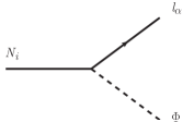
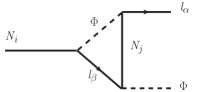
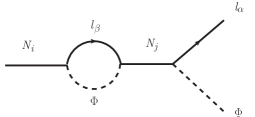
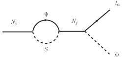
Figure 1: Tree level, vertex and the self energy diagrams required for the generation of the asymmetry in the lepton sector

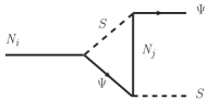
Figure 2: Tree level, vertex and the self energy diagrams required for the generation of the asymmetry in the dark sector

In Fig. 1 and Fig. 2 we present the corresponding diagrams that produce these asymmetries from RH neutrino decay. Below we express the asymmetries produced in the two sectors from the decay of the lightest RH neutrino $N_{1}$ given by,

$$\epsilon_{L} = \frac{\sum_{\alpha}[\Gamma(N_{1}\rightarrow l_{\alpha}+\Phi)-\Gamma(N_{1}\rightarrow\bar{l_{\alpha}}+\Phi^{*})]}{\Gamma_{1}}$$ (18)

$$\simeq \frac{M_{1}}{8\pi}\frac{{\rm Im}[(3Y^{*}Y^{T}+\lambda_{D}^{*}\lambda_{D}^{T})M^{-1}YY^{\dagger}]_{11}}{[2YY^{\dagger}+\lambda_{D}\lambda_{D}^{\dagger}]_{11}}\,,$$ (19)

and

$$\epsilon_{\Psi} = \frac{\Gamma(N_{1}\rightarrow\Psi+S)-\Gamma(N_{1}\rightarrow\bar{\Psi}+S^{*})}{\Gamma_{1}}$$ (20)

$$\simeq \frac{M_{1}}{8\pi}\frac{{\rm Im}[(Y^{*}Y^{T}+\lambda_{D}^{*}\lambda_{D}^{T})M^{-1}\lambda_{D}\lambda_{D}^{\dagger}]_{11}}{[2YY^{\dagger}+\lambda_{D}\lambda_{D}^{\dagger}]_{11}}\,,$$ (21)

where $\Gamma_{1}=\frac{M_{1}}{16\pi}(2YY^{\dagger}+\lambda_{D}\lambda_{D}^{\dagger})_{11}$ is the total decay width of $N_{1}$ and we have employed Eq.(1). Since we have a single generation of $\Psi$, a $3\times 3$ structure of $\lambda_{D}$ matrix can be taken to be of the form,

$${\lambda_{D}}=\left(\begin{array}[]{ccc}\lambda_{D1}&0\,~{}0\\ \lambda_{D2}&0\,~{}0\\ \lambda_{D3}&0\,~{}0\\ \end{array}\right).\,\,$$ (25)

Note that in the expression for $\epsilon_{L}$ and $\epsilon_{\Psi}$, the Yukawa couplings involved ($Y$) are also part of light neutrino mass matrix which is generated by one loop radiative correctionMa (2006) as shown in Fig. 3.

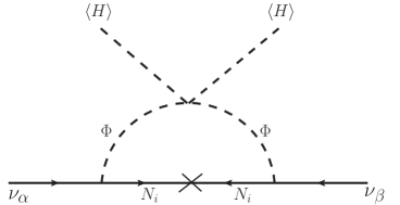
Figure 3: One-loop generation of neutrino mass.

The light neutrino mass in our set-up is given by Ahriche et al. (2018)

$$(m_{\nu})_{\alpha\beta}=\sum_{i}\frac{Y_{i\alpha}Y_{i\beta}M_{i}}{{32}\pi^{2}}\bigg{[}\frac{m_{\Phi_{0}}^{2}}{m_{\Phi_{0}}^{2}-M_{i}^{2}}{\rm{ln}}\frac{m_{\Phi_{0}}^{2}}{M_{i}^{2}}-\frac{m_{A_{0}}^{2}}{m_{A_{0}}^{2}-M_{i}^{2}}{\rm{ln}}\frac{m_{A_{0}}^{2}}{M_{i}^{2}}\bigg{]},$$ (26)

where expressions of $m_{\Phi_{0}}$ and $m_{A_{0}}$ can be obtained from Eq. (8). The mass eigenvalues and mixing are then obtained by diagonalizing the light neutrino mass matrix as:

$$m_{\nu}=U^{*}(m_{\nu}^{d})U^{\dagger}$$

with $m_{\nu}^{d}={\rm{diag}}(m_{1},m_{2},m_{3})$ consisting of mass eigenvalues and $U$ is the Pontecorvo-Maki-Nakagawa-Sakata (PMNS) matrix Maki et al. (1962) (the charged lepton mass matrix is considered to be diagonal) which can be written as:

$$U=\left(\begin{array}[]{ccc}c_{12}c_{13}&c_{13}s_{12}&e^{-i\delta_{CP}}s_{13}\\ -c_{23}s_{12}-e^{i\delta_{CP}}c_{12}s_{13}s_{23}&c_{12}c_{23}-e^{i\delta_{CP}}s_{12}s_{13}s_{23}&c_{13}s_{23}\\ s_{12}s_{23}-e^{i\delta_{CP}}c_{12}c_{23}s_{13}&-e^{i\delta_{CP}}c_{23}s_{12}s_{13}-c_{12}s_{23}&c_{13}c_{23}\\ \end{array}\right)\times{\rm{diag}}(e^{i\alpha_{1}/2},e^{i\alpha_{2}/2},1),$$

where $\theta_{12},\theta_{23},\theta_{13}$ are the mixing angles ($c_{ij}=\cos\theta_{ij},s_{ij}=\sin\theta_{ij}$). Dirac CP phase is $\delta_{CP}$ and Majorana CP phases are denoted by $\alpha_{1},\alpha_{2}$. For simplicity we will consider the Majorana phases to be zero. The best fit values of these parameters along with their 3$\sigma$ ranges are mentioned in Table 2.

V Boltzmann Equations

In this section we present the Boltzmann equations that lead to the final lepton asymmetry and dark matter abundance. As we have mentioned earlier, asymmetries in both the sectors are generated from the decay of the lightest right handed Majorana neutrinos $N_{1}$ (in this work the right handed Majorana neutrinos follow a hierarchical structure $M_{1}<M_{2}<M_{3}$). Once the lepton and dark matter asymmetries ($\epsilon_{L}$ and $\epsilon_{\Psi}$) are obtained via Eqs. (19) and (21), their evolution can be studied by a set of Boltzmann equations involving all the relevant interactions. This is represented by the abundance yields $Y_{j}=\frac{n_{j}}{s}$ ($j=N_{1},x$ with $x=l,\Psi$), $n_{j}$ being the respective number density of particle $j$ and $s$ is the entropy density at certain temperature $T$. Then denoting $Y_{\Delta L}=Y_{l}-Y_{\bar{l}}$ and $Y_{\Delta\Psi}=Y_{\Psi}-Y_{\bar{\Psi}}$, the Boltzmann equations involving the corresponding quantities become Falkowski et al. (2011)

$$\frac{dY_{N_{1}}}{dz} = -z\frac{\Gamma_{1}}{H_{1}}\frac{K_{1}(z)}{K_{2}(z)}\left(Y_{N_{1}}-Y_{N_{1}}^{\rm eq}\right)\,\,,$$ (28)

$$\frac{dY_{\Delta x}}{dz} = \frac{\Gamma_{1}}{H_{1}}\left(\epsilon_{x}z\frac{K_{1}(z)}{K_{2}(z)}(Y_{N_{1}}-Y_{N_{1}}^{eq})-Br_{x}\frac{z^{3}K_{1}(z)}{4}Y_{\Delta x}\right)\,,(x=L,\Psi).$$ (29)

Here $Y_{N_{1}}^{\rm eq}$ represents the equilibrium abundance of $N_{1}$ and $z$ is given by $z=\frac{M_{1}}{T}$. $H_{1}$ is the Hubble parameter at $T=M_{1}$. $K_{i}(z),~{}i=1,2$ are the modified Bessel functions of first and second kinds respectively and $Br_{x}$ denotes the branching ratios of $N_{1}$ decay into the SM and dark sectors.

The evolution of the lightest RHN $N_{1}$ abundance due to its decay and inverse decay is described by Eq. (28). Here, $\frac{\Gamma_{1}}{H_{1}}$ illustrates the strength of these interactions and controls the departure of $N_{1}$ from thermal equilibrium. Eq. (29) describes the evolution of the asymmetries generated in both visible as well as the dark sectors. The term proportional to $\epsilon_{L(\Psi)}$ is responsible for the production of the asymmetry $Y_{\Delta L({\Delta\Psi})}$ once $N_{1}$ drops out of thermal equilibrium whereas the second term (in the first bracketed term of r.h.s of Eq. (29)) proportional to $Br_{L(\Psi)}$ is responsible for the washout of the asymmetries due to the inverse decay of $N_{1}$.

In principle, the final yields of lepton (matter) as well as dark matter should be obtained by solving the coupled Boltzmann equations. However here they turn out to be independent (see Eq. (29)) due to our consideration of narrow width approximation. Using the relevant neutrino Yukawa coupling (turns out to be below $\mathcal{O}(1)$) and so with $\lambda_{D1}$ (see Sec. VI for detail), we find that $\frac{\Gamma_{1}}{M_{1}}<<1$ with RH neutrino mass $M_{1}$ being $10^{9}$ GeV or above. We further find that with sufficiently large RH neutrino mass $M_{1}\sim 10^{12}~{}\rm{GeV}$ (as in this work), the other requirement for realizing narrow width approximation, $i.e.$, $\frac{\Gamma_{1}^{2}}{M_{1}H_{1}}<1$ is also satisfied. Such a choice of heavy RH neutrino mass is also consistent with Davidson Ibarra (DI) bound Davidson and Ibarra (2002) and allows us not to consider the flavor effects in the analysis. Within this approximation, the $2\leftrightarrow 2$ transfer ($l\Phi\leftrightarrow\bar{\Psi}S,~{}l\Phi\leftrightarrow\Psi S,~{}\bar{l}\Phi^{\dagger}\leftrightarrow\bar{\Psi}S,~{}\bar{l}\Phi^{\dagger}\leftrightarrow\Psi S$ and washout terms ($l\Phi\leftrightarrow\bar{l}\Phi^{\dagger},~{}\bar{\Psi}S\leftrightarrow\Psi S$, where $S$ is a real scalar) mediated by RHNs are neglected. Therefore, transfer of asymmetries between the SM and dark sectors are absent. However the presence of $2\rightarrow 1$ inverse decay processes ( $l\Phi,\bar{l}\Phi^{\dagger}\rightarrow N_{1}$ and $\Psi S,~{}\bar{\Psi}S\rightarrow N_{1}$) are included through the term proportional to $Br_{x}$, which corresponds to the washout of asymmetries.

Finally a part of the lepton asymmetry (yield $Y_{\Delta L}$) is further converted into the baryon asymmetry ($i.e.$ to the yield of $Y_{\Delta B}$) via Sphaleron transition (see Davidson et al. (2008) and references therein). On the other hand, since Sphaleron does not interact with dark sector, dark sector asymmetry will not be converted. Considering the Spahleron is in equilibrium above the electroweak phase transition (EWPT) temperature Davidson et al. (2008)-Buchmuller et al. (2005b), the net baryon asymmetry can be expressed as Davidson et al. (2008)

$$Y_{\Delta B}=\frac{8}{23}Y_{\Delta L}\,.$$ (30)

We now denote the final yields of the lepton and the dark sector (obtained by solving the Boltzmann equations) at present temperature $T_{0}$ by $Y_{\Delta L}^{0}$ and $Y_{\Delta\Psi}^{0}$ respectively. In order to satisfy the observed baryon asymmetry in the Universe $Y_{\Delta B}^{0}=(8.24-9.38)\times 10^{-11}$Tanabashi et al. (2018), $Y_{\Delta L}^{0}$ must be within the range $(2.37-2.70)\times 10^{-10}$. The relic abundance of dark matter follows the relation Edsjo and Gondolo (1997)

$$\Omega_{\Psi}h^{2}=2.755\times 10^{8}\left(\frac{m_{\Psi}}{{\rm{GeV}}}\right)Y_{\Delta\Psi}^{0}\,.$$ (31)

The asymmetric dark matter candidate $\Psi$ has no other interaction except the one in Eq. (1) and therefore it decouples from thermal bath once the decay of right handed neutrino completed. However, the other decay products of $N_{1}$ such as the scalar $S$ and inert Higgs doublet remain in thermal equilibrium. It is to be noted that any asymmetry in the inert Higgs doublet (as a decay product) is expected to be restored fast due to its copious interactions and hence its number density reaches equilibrium satisfying the condition $n^{eq}_{\Phi}=n^{eq}_{\Phi^{\dagger}}$. Also, $S$ being a real scalar, any asymmetry in $S$ is redundant. However as the temperature of the Universe decreases, it may leave us a symmetric dark matter component ($\Phi_{0}$) too which decouples at some lower temperature from the thermal bath when thermal annihilation freezes out. Such a contribution would provide an additional contribution to the relic in the set-up.

The relic abundance of the symmetric dark matter can be obtained by solving Boltzmann equation

$$\frac{dY_{\Phi_{0}}}{dz^{\prime}} = -\frac{1}{z^{\prime 2}}\langle\sigma v_{\Phi_{0}\Phi_{0}\rightarrow XX}\rangle\left(Y_{\Phi_{0}}^{2}-(Y_{\Phi_{0}}^{eq})^{2}\right)\,,$$ (32)

where $z^{\prime}=m_{\Phi_{0}}/T$ and $Y_{\Phi_{0}}^{eq}$ denotes equilibrium number density of $\Phi_{0}$. The relic density of inert scalar $\Phi_{0}$ is then expressed as

$$\Omega_{\Phi_{0}}h^{2}=2.755\times 10^{8}\left(\frac{m_{\Phi_{0}}}{{\rm{GeV}}}\right)Y_{\Phi_{0}}^{0}\,.$$ (33)

Therefore in the present framework, one must satisfy the condition for total DM relic abundance

$$\Omega_{\rm DM}h^{2}=\Omega_{\Psi}h^{2}+\Omega_{\Phi_{0}}h^{2}\,.$$ (34)

VI Strategy for evaluating $\epsilon_{L}$ and $\epsilon_{\Psi}$

In order to obtain initial values of $\epsilon_{L}$ and $\epsilon_{\Psi}$ via Eqs. (19) and (21), we note that evaluations of $Y$ matrix, $\lambda_{D_{i}}$ and $M_{1}$ are required. The same $Y$ being involved in neutrino mass matrix $m_{\nu}$ via Eq. (26) must be evaluated so as to obey the constraints on neutrino parameters (see section III). On the other hand, $\lambda_{D_{i}}$ turn out to be free parameters. For simplicity, we consider the source of CP violation to follow only from the complex neutrino Yukawa coupling ($Y$). Hence $\lambda_{D_{i}}$ are considered to be real. We further assume all three $\lambda_{D_{i}}$ are same, denoted by $\lambda_{D}$. As discussed before, to generate lepton asymmetry, dark matter and neutrino mass, we rely here on heavy RH neutrinos having mass $\sim 10^{9}$ GeV and above so as to satisfy the narrow width approximation and the DI bound.

The remaining ingredient is to find out whether the asymmetric component is the sole contribution to the dark matter relic or there could be a subdominant, but non-negligible, symmetric contribution to follow from IHD. In determining this, we note that the relic abundance $\Phi_{0}$ depends on mass splitting between the particles of the inert multiplet: $\Delta M=m_{(\Phi^{\pm},A^{0})}-m_{\Phi_{0}}$. Keeping in mind that we mostly focus on the intermediate mass range for the IHD, it results under-abundance of relic density with $\Delta M\sim\mathcal{O}(1)$ GeV. As a limiting case, with sufficiently large $\Delta M$, the contribution seems to be negligible and we may end up having the dark matter abundance constituted only by the asymmetric component from $\Psi$. However as we will see below that such a large $\Delta M$ poses a threat to the high scale validity. Hence a balance is required in choosing $\Delta M$ in our scenario so as to keep the IHD’s contribution to relic small and simultaneously the stability of the set-up till a large scale can be achieved.

VI.1 Determination of $Y$

We understand that the neutrino Yukawa coupling $Y$ plays vital role in determining the neutrino mass as well as asymmetries $\epsilon_{L}$ and $\epsilon_{\Psi}$. The neutrino mass expressed in Eq. (26), can be redefined as

$$({m_{\nu}})_{\alpha\beta}=(Y\Lambda Y^{T})_{\alpha\beta}\,\,$$ (35)

where $\Lambda=\rm{diag}(\Lambda_{1},\Lambda_{2},\Lambda_{3})$ and $\Lambda_{i}$ (for i=1,2,3) is expressed by

$$\Lambda_{i} = \bigg{[}\frac{M_{i}}{{32}\pi^{2}}\bigg{(}\frac{m_{\Phi_{0}}^{2}}{m_{\Phi_{0}}^{2}-M_{i}^{2}}{\rm{ln}}\frac{m_{\Phi_{0}}^{2}}{M_{i}^{2}}-\frac{m_{A_{0}}^{2}}{m_{A_{0}}^{2}-M_{i}^{2}}{\rm{ln}}\frac{m_{A_{0}}^{2}}{M_{i}^{2}}\bigg{)}\bigg{]}.$$ (36)

Note that within $\Lambda$, parameters $m_{\Phi_{0}},m_{A_{0}}$ are part of the DM phenomenology. Therefore with their fixed values, $\Lambda$ would only be a function of $M_{i}$ which can be evaluated with a choice of $M_{1}$ and a fixed mass ratio of RHNs (we consider hierarchical RHNs). Afterward, we use the Casas-Ibarra (CI) parametrization Casas and Ibarra (2001) to evaluate the Yukawa couplings via

$$Y = \sqrt{\Lambda^{-1}}R\sqrt{m^{d}_{\nu}}U^{\dagger},\,$$ (37)

where $R$ is a complex orthogonal matrix $R^{T}R=1$, taken as

$$R=\begin{pmatrix}0&\cos{z}&\sin{z}\\ 0&-\sin{z}&\cos{z}\\ 1&0&0\\ \end{pmatrix}\hskip 14.22636pt \text{for NH}\,, \hskip 28.45274ptR=\begin{pmatrix}\cos{z}&-\sin{z}&0\\ \sin{z}&\cos{z}&0\\ 0&0&1\\ \end{pmatrix}\hskip 14.22636pt$$ for IH , (38)

with $z=z_{R}+iz_{I}$, a complex number. In order to obtain $m_{\nu}^{d}=diag(m_{1},m_{2},m_{3})$, we consider the lightest neutrino mass eigenvalue to be zero with $m_{1}=0$ ($m_{1}<m_{2}<m_{3}$) for NH and $m_{3}=0$ ($m_{3}<m_{1}<m_{2}$) for IH. Then $m_{\nu}^{d}$ is calculable using the best fit values of solar and atmospheric mass splittings of Table 2. Therefore, elements of Yukawa coupling matrix, $Y_{i\alpha}$, for a specific $z$ value can be easily obtained for different choices of model parameters $m_{\Phi_{0}},~{}\Delta M,~{}M_{1}$, ratio of RHN masses etc.

VI.2 Fixing $\Delta M$

By knowing the elements of neutrino Yukawa coupling, $Y_{i\alpha}$, we are now able to calculate initial asymmetries, $\epsilon_{\Psi}$ and $\epsilon_{L}$. Now following the discussion in the beginning of this section, we plan to discuss the suitable choice of $\Delta M$ as it controls the high scale validity, $i.e.$ perturbativity and vacuum stability, of the present construction. In doing that, we recall that the top Yukawa coupling $y_{t}\sim\mathcal{O}(1)$, drags the Higgs quartic coupling towards the negative value at a scale around $10^{10}$ GeV in the SM Buttazzo et al. (2013); Degrassi et al. (2012); Tang (2013); Ellis et al. (2009); Elias-Miro et al. (2012) which is suggestive of a metastable EW vacuum within the present $3\sigma$ limits of $m_{t}$ Tanabashi et al. (2018). Involvement of the new scalar degree of freedoms like IHD and scalar singlet in the present scenario can modify the fate of EW vacuum as the running of the Higgs quartic coupling $\lambda_{H}$ would be affected by their presence. On the other hand, due to the presence of heavy RHNs, we must ensure that the couplings involved should obey the stability and pertubativity conditions (see Eq. (9), $\lambda_{i}<4\pi$) at least up to the highest RHN mass scale. As we will see, choice of $\Delta M$ would be crucial in this regard.

VI.2.1 Vacuum stability

For this purpose, we first study the running of different couplings of the model. Beta functions of all such coupling are provided in Appendix A. The modification of the beta function of $\lambda_{H}$ (through their Higgs portal coupling) can be expressed (at one loop) as:

$$\beta_{\lambda_{H}} =\beta_{\lambda_{H}}^{\rm{SM}}+\beta_{\lambda_{H}}^{\rm{IHD}}+\beta_{\lambda_{H}}^{\rm{S}}~{}=~{}\beta_{\lambda_{H}}^{\rm{SM}}+2\lambda_{1}^{2}+2\lambda_{1}\lambda_{2}+\lambda_{2}^{2}+\lambda_{3}^{2}+\frac{1}{2}\lambda^{2}_{HS}$$ (39)

The condition, $\lambda_{H}>0$ till the Planck scale ($M_{Pl}$) ensures the absolute stability of the EW vacuum, if violated at any scale below $M_{Pl}$ the EW vacuum can become metastable or unstable. Now, if the Higgs quartic coupling $\lambda_{H}(\mu)$ turns negative at any scale (as happens for SM at $\mu\sim 10^{9-10}$ GeV), there may exist another deeper minimum other than the EW one. In such a scenario, one requires to confirm the metastability of the Higgs vacuum by estimating the tunneling probability $\mathcal{P}_{T}$ of the EW vacuum to the second minimum such that the associated decay time is longer than the age of the Universe. The tunneling probability is given by Isidori et al. (2001); Buttazzo et al. (2013),

$$\mathcal{P}_{T}=T^{4}_{U}\mu_{B}^{4}e^{-\frac{8\pi^{2}}{3|\lambda_{H}(\mu_{B})|}},$$ (40)

where $T_{U}$ is the age of the Universe, $\mu_{B}$ is the scale at which the tunneling probability is maximized, determined from $\beta_{\lambda_{H}}(\mu_{B})=0$. Solving the above equation, the metastability requires: $\lambda_{H}(\mu_{B})>-0.065/[1-\rm{ln}\big{(}\frac{v}{\mu_{B}}\big{)}]$.

At high energies, one can write the RG improved effective potential as Degrassi et al. (2012)

$$V^{\rm{eff}}_{H} = \frac{\lambda^{\rm{eff}}_{H}(\mu)}{4}h^{4},$$ (41)

where $\lambda^{\rm{eff}}_{H}(\mu)=\lambda^{\rm{SM,eff}}_{H}(\mu)+\lambda^{\rm{IHD},\rm{eff}}_{H}(\mu)+\lambda^{\rm{S,eff}}_{H}(\mu)$. Here, $\lambda^{\rm{SM,eff}}_{H}(\mu)$ is the contribution coming from the SM fields to $\lambda_{H}$ whereas $\lambda^{\rm{IHD,eff}}_{H}(\mu)$ and $\lambda^{\rm{S,eff}}_{H}(\mu)$ are contribution to the $\lambda_{H}$ coming from the IHD ($\Phi$) and the scalar singlet ($S$) in the current setup. These new contributions can be expressed as:

$$\lambda^{\rm{IHD,eff}}_{H}(\mu) = e^{4\Gamma(h=\mu)}\frac{1}{16\pi^{2}}\bigg{[}2\frac{\lambda_{1}^{2}}{4}\bigg{(}\rm{ln}\frac{\lambda_{1}}{2}-\frac{3}{2}\bigg{)}+\frac{(\lambda_{1}+\lambda_{2}+\lambda_{3})^{2}}{4}\bigg{(}\rm{ln}\frac{\lambda_{1}+\lambda_{2}+\lambda_{3}}{2}-\frac{3}{2}\bigg{)}$$ (42a)

$$+ \frac{(\lambda_{1}+\lambda_{2}-\lambda_{3})^{2}}{4}\bigg{(}\rm{ln}\frac{\lambda_{1}+\lambda_{2}-\lambda_{3}}{2}-\frac{3}{2}\bigg{)}\bigg{]},$$

$$\lambda^{\rm{S,eff}}_{H}(\mu) = e^{4\Gamma(h=\mu)}\frac{1}{16\pi^{2}}\bigg{[}\frac{\lambda^{2}_{HS}}{4}\bigg{(}\rm{ln}\frac{\lambda_{HS}}{2}-\frac{3}{2}\bigg{)}\bigg{]}.$$ (42b)

Here, $\Gamma(h)=\int_{m_{t}}^{h}\gamma(\mu)~{}\rm{d~{}ln(\mu)}$ and $\gamma(\mu)$ is the anomalous dimension of the Higgs field Buttazzo et al. (2013).

Scale	$\lambda_{H}$	$y_{t}$	$g_{1}$	$g_{2}$	$g_{3}$
$\mu=m_{t}$	$0.125932$	$0.93610$	$0.357606$	$0.648216$	$1.16655$

Table 3: Values of the relevant SM couplings (top-quark Yukawa $y_{t}$ , gauge couplings $g_{i}(i=1,2,3)$ and Higgs quartic coupling $\lambda_{H}$ ) at energy scale $\mu=m_{t}=173.2$ GeV with $m_{h}=125.09$ GeV and $\alpha_{S}(m_{Z})=0.1184$.

For the stability analysis purpose, we choose $\mu=m_{t}$ as an initial scale and the running of the scalar couplings (inclusive of $\lambda_{H}$ and other relevant scalar couplings in the set-up) is done at two-loops till $M_{Pl}$. Since RHNs do not couple to the SM Higgs, it does not affect the running of $\lambda_{H}$ and other scalar couplings significantly and hence for this part of analysis, we do not consider the presence of RHNs. In table 3, we provide the initial conditions of relevant SM couplings at $\mu=m_{t}$ Buttazzo et al. (2013). Here, we consider $m_{h}=125.09$ GeV, $m_{t}=173.2$ GeV, and $\alpha_{S}(m_{Z})=0.1184$. For scalar couplings such as $\lambda_{1,2,3}$ we use the following relations of them with the mass parameters (see Eq. (8)) given by,

$$\lambda_{1} = 2\lambda_{L}+\frac{2(m_{\Phi^{+}}^{2}-m_{\Phi_{0}}^{2})}{v^{2}},$$ (43a)

$$\lambda_{2} = \frac{m_{\Phi_{0}}^{2}+m_{A_{0}}^{2}-2m_{\Phi^{+}}^{2}}{v^{2}},$$ (43b)

$$\lambda_{3} = \frac{(m^{2}_{\Phi_{0}}-m^{2}_{A_{0}})}{v^{2}}.$$ (43c)

Note that the mass splitting $\Delta M$ controls the values of these scalar couplings (we consider $\lambda_{2}=\lambda_{3}$). Since we are interested in keeping the IHD’s mass in the intermediate range, we choose $m_{\Phi_{0}}$ to be 300 GeV and $\lambda_{L}=0.01$ as a benchmark values and consider $\Delta M$ as the parameter to be varied. We consider portal couplings $\lambda_{HS}=\lambda_{\Phi S}=0.001$ so that effect of $\Delta M$ on the running of $\lambda_{H}$ and the other quartic couplings becomes prominent.

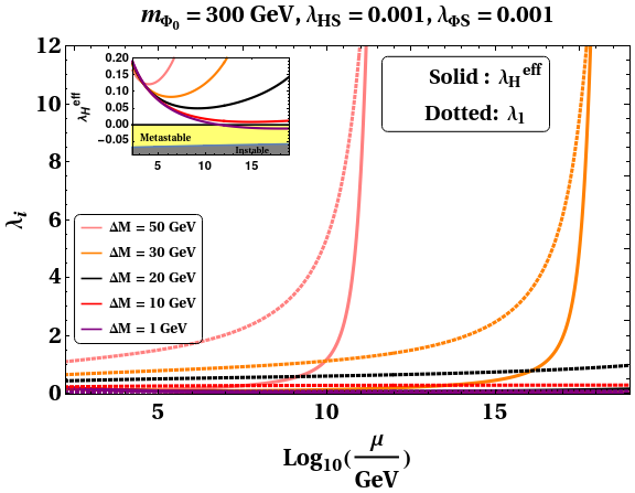
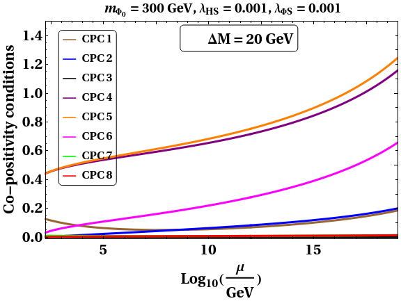
Figure 4: Left panel: Evolution of effective Higgs quartic coupling ($\lambda_{H}^{\rm eff}$) and $\lambda_{1}$ against the scale $\mu$, Right panel: Evolution of all the copositivity conditions (Eq.9) against the scale $\mu$ . In both the plots we have kept $m_{\Phi_{0}}=300$ GeV, $\lambda_{L}=0.01$, $\lambda_{HS}=0.001$ and $\lambda_{\Phi S}=0.001$ .

In Fig.4 (a), we show the evolution of the couplings $\lambda_{H}^{\rm eff}$ (solid line) and $\lambda_{1}$ (dotted line) with the energy scale $\mu$ for the different choices of mass splittings: $\Delta M$ = 50 GeV (pink), 30 GeV (orange), 20 GeV (black), 10 GeV (red) and 1 GeV (purple). One finds that for $\Delta M=30$ GeV and above, the coupling $\lambda_{1}$ becomes non-perturbative ($\lambda_{1}(\mu)>4\pi$) well before the $M_{pl}$. This is because for $\Delta M=30$ GeV itself, $\lambda_{1}$ turns out to be quite large, $\sim\mathcal{O}(0.6)$ at $\mu=m_{t}$. However, the values of the coupling $|\lambda_{2}|$ (or $|\lambda_{3}|$) is found to be $\sim\mathcal{O}(0.3)$ at $m_{t}$ and it remains perturbative till $M_{pl}$. In this plot, we also provide evolution of the effective Higgs quartic coupling $\lambda_{H}^{\rm eff}$. Due to the involvement of term proportional to $\lambda_{1}^{2}$ (also significant contribution follows from $\lambda_{2,3}^{2}$) as seen in Eq. (39), the rapid increase of $\lambda_{H}^{\rm eff}$ is observed for $\Delta M=30$ GeV (and above). This observation suggests that we need to keep our choice of $\Delta M$ below 30 GeV. Note that with $\Delta M$ below 10 GeV, the EW vacuum remains metastable (yellow shade region) as shown in the inset figure of the left panel. In the right panel, Fig.4 (b), we show that all the co-positivity conditions (discussed in Eq. (9)) are maintained till the Planck scale with a choice $\Delta M=20$ GeV.

VI.2.2 Relic contribution from IHD

As we have already discussed, we aim for asymmetric DM in this work to satisfy the entire relic. However, involvement of the IHD in the set-up naturally puts the question whether there can be any symmetric DM contribution to the relic. In this regard we know that the relic of the IHD doublet remains under abundant in the mass regime we are interested in, $i.e.~{}80-500$ GeV. This is due to the fact that IHD being a $SU(2)$ doublet it can annihilate into the SM gauge bosons ($W^{+},Z$) with a large cross-section. Beyond this range, the relic satisfaction by the lightest component of IHD happens with small $\Delta M\sim\mathcal{O}(1)$ GeV.

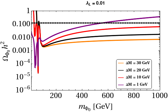
Figure 5: Variation of the relic density $\Omega_{\Phi_{0}}h^{2}$ of the IHD with its mass $m_{\Phi_{0}}$ keeping $\lambda_{L}=0.01$ for different values of $\Delta M$.

In Fig 5, we show the variation of the relic density ($\Omega_{\Phi_{0}}h^{2}$) with its mass $m_{\Phi_{0}}$ for different values of $\Delta M$. It is seen that with the increase of $\Delta M$, its contribution towards the total relic of the dark matter decreases. More precisely, we note that with $\Delta M$ = 20 GeV (30 GeV), it can contribute maximum of $6\%$ ($3\%$) towards the total relic density of the dark matter at $m_{\Phi_{0}}=300$ GeV. Hence combining our understanding related to vacuum stability issue and to minimize the symmetric contribution from IHD to DM relic, we choose to work with $\Delta M$ range: 10-30 GeV. Effect of $\Delta M$ in having the lepton asymmetry and asymmetric DM generation are part of our study in the following section.

It is also interesting to point out that in an IHD scenario DM mass below 400 GeV is ruled out by Fermi-LAT constraints Borah and Gupta (2017). However, IHD being the less abundant DM candidate as in this work, effective IHD annihilation cross-section for indirect detection is rescaled by a factor $\left(\frac{\Omega_{\Phi_{0}}h^{2}}{\Omega_{\rm DM}h^{2}}\right)^{2}$ Borah et al. (2019); Bhattacharya et al. (2020a) and as a result limits from Fermi-LAT becomes insignificant.

VII Results and discussion

In this section, we present the results for the final yields of the lepton and the dark asymmetries obtained by solving the Boltzmann equations and investigate whether it can provide the required baryon asymmetry and dark matter abundance in order to satisfy the observed bounds. Simultaneously, we study how things change with different neutrino mass hierarchies. For this purpose, we use the neutrino Yukawa couplings obtained using CI parametrization with (i) given values of heavy right handed neutrino masses, and (ii) inert doublet parameters: $m_{{\Phi}_{0}}$ and $\Delta M$. The other coupling required to solve the Boltzmann equations are the dark sector Yukawa couplings $\lambda_{Di},~{}i=1,2,3$. As already stated, we assume $\lambda_{D_{i}}$ to be real and same, denoted by $\lambda_{D}$. It is interesting to mention that although we consider $\lambda_{D}$ to be real, a finite asymmetry in the dark sector $\epsilon_{\Psi}$ follows from the involvement of complex neutrino Yukawa couplings $Y$. As a result of it, there will not be any contribution from Fig. 2(b) and  2(d). Under this circumstances, the Eq. (21) reduces to

$$\epsilon_{\Psi}=\frac{M_{1}}{8\pi}\frac{{\rm Im}[Y^{*}Y^{T}M^{-1}\lambda_{D}\lambda_{D}^{\dagger}]_{11}}{[2YY^{\dagger}+\lambda_{D}\lambda_{D}^{\dagger}]_{11}}\,.$$ (44)

As stated in Sec.VI, for a given set of neutrino parameters given in Table 2 (normal or inverted hierarchy), one can obtain Yukawa couplings $Y_{i\alpha}$ for different choices of model parameters $\Delta M,~{}m_{\Phi_{0}}$, RHN mass and CI parameter $z$ using Eqs. (35-38). Varying the other parameter $\lambda_{D}$ (dark sector coupling), asymmetries in lepton and dark sectors $\epsilon_{L,\Psi}$ (using Eqs. (19) and (21)), total decay width of lightest RHN $\Gamma_{1}$ and its branching ratios to visible and dark sectors, $Br_{L,\Psi}$ are obtained. We then use $\epsilon_{L,\Psi}$, $\Gamma_{1}$ and $Br_{L,\Psi}$ to solve the Boltzmann equations (Eqs. (28-29)) and obtain the final comoving density $Y^{0}_{\Delta B,\Delta\Psi}$ at present temperature $T_{0}$ for each value of $\lambda_{D}$.

Our aim is to find out the relevant parameter space of the model which satisfies the correct baryon number density and dark matter relic abundance. This helps us to identify the corresponding allowed ranges of dark matter mass. While investigating the yields of lepton and dark asymmetries against $\lambda_{D}$ variation, we keep on changing other parameters as well, however one at a time, $i.e.$ changing a) mass splitting $\Delta M$, and b) different RHNs mass ratio.

VII.1 Case of NH

Using the prescription stated above, we first evaluate Yukawa couplings for NH case for a specific set of parameters

$$z_{R}=0.030,~{}z_{I}=-0.086,~{}m_{\Phi_{0}}=300~{}{\rm GeV},M_{1}=10^{12}~{}{\rm GeV}.$$ (45)

Note that, as stated before, this benchmark value of $m_{\Phi_{0}}$ is motivated by the fact that we are interested to keep the IHD within the intermediate mass range. We also consider heavy RHNs and $10^{12}$ GeV is only a representative value. However, choosing such high value, we can safely ignore the flavor effects Abada et al. (2006a); Nardi et al. (2006); Abada et al. (2006b); Blanchet and Di Bari (2007); Blanchet et al. (2007); Dev et al. (2018b). Then with $\Delta M=20$ GeV and a fixed ratio of RHN masses, $M_{1}:M_{2}:M_{3}=1:10:100$, using Eq. (37) we obtain,

$$Y=\begin{pmatrix}0.0388759-0.00119665i&0.0545874-0.0042563i&-0.0314376-0.00486761i\\ -0.0423476-0.0692572i&0.343607+0.00173362i&0.405694-4.97426\times 10^{-6}i\end{pmatrix}.\hskip 14.22636pt$$ (46)

We will also choose different sets of $\Delta M$ and mass ratio and correspondingly different $Y$ matrix would follow. Throughout the work, solution to Boltzmann equations are obtained with $\lambda_{D}$ range $10^{-4}-10^{-1}$. We note that condition for narrow width approximation, $\frac{\Gamma_{1}^{2}}{M_{1}H_{1}}\ll 1$, mentioned in Sec. V is valid for such chosen range of $\lambda_{D}$.

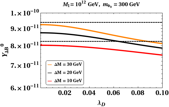
(a) Lepton Sector

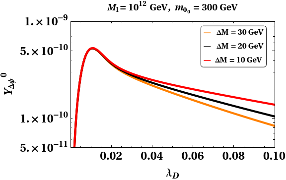
(b) Dark Sector

Figure 6: Variation of asymptotic yield $Y_{\Delta B}^{0}$ and $Y_{\Delta\Psi}^{0}$ with the dark sector Yukawa coupling $\lambda_{D}$ for $\Delta M=10~{}{\rm GeV},~{}20~{}{\rm GeV},~{}30~{}{\rm GeV}$.

In Fig. 6(a) and (6b), we plot the variation $Y_{\Delta B}^{0}$ ($Y_{\Delta\Psi}^{0}$) against $\lambda_{D}$ (after solving the Boltzmann equations) for different set of values of $\Delta M$ = 10, 20 and 30 GeV associated with the above benchmark set of parameters in Eq. (45). Here ratio of the RHN masses is taken as $M_{1}:M_{2}:M_{3}=1:10:100$. The horizontal black dashed lines in Fig. 6(a) represents the correct abundance yield of $Y_{\Delta B}^{0}$ today followed from the observed baryon asymmetry in the UniverseAde et al. (2016). From Fig. 6(a), we notice that for $\Delta M=20$ GeV ($\Delta M=30$ GeV) baryon abundance in Universe is satisfied with $\lambda_{D}\leq 0.065$ ($\lambda_{D}\leq 0.09$). However, for $\Delta M=10$ GeV, $Y_{\Delta B}^{0}$ turns out to be inadequate for the entire range of $\lambda_{D}$ considered. Similarly, in the right panel we provide plots of variation of $Y_{\Delta\Psi}^{0}$ against $\lambda_{D}$ with different values of $\Delta M$.

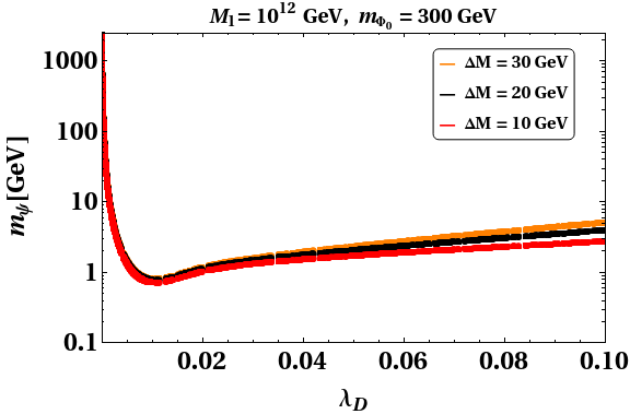
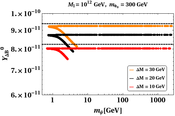
Figure 7: Left panel: Variation the asymmetric dark matter mass $m_{\Psi}$ with the dark sector Yukawa coupling $\lambda_{D}$, Right panel: Variation of asymptotic yield $Y_{\Delta B}^{0}$ with the dark matter mass $m_{\Psi}$. Both the plots are shown for $\Delta M=10~{}{\rm GeV},~{}20~{}{\rm GeV},~{}30~{}{\rm GeV}$.

In order to understand the patterns observed in Fig. 6, we first note that r.h.s of the Boltzmann equation for $Y_{\Delta L}$ (see Eq. (29)) contains two terms, one is $\epsilon_{L}$ dependent and the other one is washout related, proportional to $Br_{\Psi}$. Since $Y$ is fixed, the nature of $Y_{\Delta B}^{0}$ against $\lambda_{D}$ is mostly governed by the $\epsilon_{L}$-related (first) term. Now from the expression of $\epsilon_{L}$ as in Eq. (20), we note its variation with $\lambda_{D}$ is insignificant due to the presence of $\lambda_{D}$ in both numerator and denominator. Hence a near to flatness is observed in left panel of Fig. 6(a). On the other hand, in case of dark sector, although the first term in the r.h.s. of corresponding Boltzmann equation for $Y_{\Delta L}$ dominates over the second term for small $\lambda_{D}$, the contribution form second term (proportional to $Br_{\Psi}$) increases with increasing $\lambda_{D}$ leading to large washout effects. As a result, when washout effect is negligible in dark sector, $Y_{\Delta\Psi}^{0}$ increases rapidly with increasing $\lambda_{D}$ as expected from Eq. (44). This situation alters with higher $\lambda_{D}$ (beyond $\lambda_{D}\sim 0.01$) where a significant washout happens with further increase of $\lambda_{D}$ (associated to larger $Br_{\Psi}$). This produces an overall mild falling nature of $Y_{\Delta\Psi}^{0}$ against $\lambda_{D}$ as observed in Fig. 6(b) (for $\lambda_{D}>0.01$) which now becomes distinguishable for different $\Delta M$ values.

In Fig. 7(a), we plot the correlation between $m_{\Psi}$ and $\lambda_{D}$ for different choices of $\Delta M$. This correlation is simply obtained from the right panel of Fig. 6 by taking into account: (i) the required asymmetric contribution to DM relic from $\Psi$ ($\Omega_{\Psi}h^{2}$) corresponding to any value of $\lambda_{D}$ through Eq. (16) and (34) as the presence of IHD also provides a small but nonzero symmetric contribution to relic associated to specific choice of $\Delta M$; (ii) then from Fig. 6(b), we find the respective $Y_{\Delta\Psi}^{0}$ and using Eq. (31) the corresponding value of $m_{\Psi}$ is obtained. The typical nature (parabolic) of this correlation plot observed here is inherited from the right panel of Fig. 6 considering the reciprocity relation between $m_{\Psi}$ and $Y_{\Delta\Psi}^{0}$ as in Eq. (31).

Then in Fig. 7(b), we plot the correlation between dark matter mass $m_{\Psi}$ and $Y_{\Delta B}^{0}$ obtained directly from Fig. 6(a) and Fig. 7(a) for a given $\lambda_{D}$. From Fig. 6(a) and 6(b), it is observed that for $\lambda_{D}\gtrsim 0.05$ order of magnitudes of dark matter abundance and baryon asymmetry are almost similar, $Y_{\Delta\Psi}^{0}\sim Y_{\Delta B}^{0}$ and they do not change significantly with the increase of $\lambda_{D}$ beyond 0.05 resulting $m_{\Psi}\sim\mathcal{O}$ (GeV) as seen from Fig. 7(a). On the other hand, for $\lambda_{D}<0.05$, we have noticed a sharp variation in $Y_{\Delta\Psi}^{0}$ against $\lambda_{D}$ whereas $Y_{\Delta B}^{0}$ continues to exhibit the same moderate variation as observed by comparing Fig. 6(a) and 6(b) resulting in a wider range of DM masses in this case: from GeV to TeV. This is also visible from Fig. 7(a). Hence for this regime of DM mass (above GeV), $Y_{\Delta B}^{0}$ is effectively insensitive to the increase in $m_{\Psi}$ as seen in Fig. 7(b). This finding that two regions of $\lambda_{D}$ (below and above 0.05) shows different dependency on $m_{\Psi}$ is due to the interplay between the generation and wash-out of asymmetries (as discussed before) both being functions of $\lambda_{D}$ and in line with observation in Falkowski et al. (2011), a characteristic of two-sector leptogenesis.

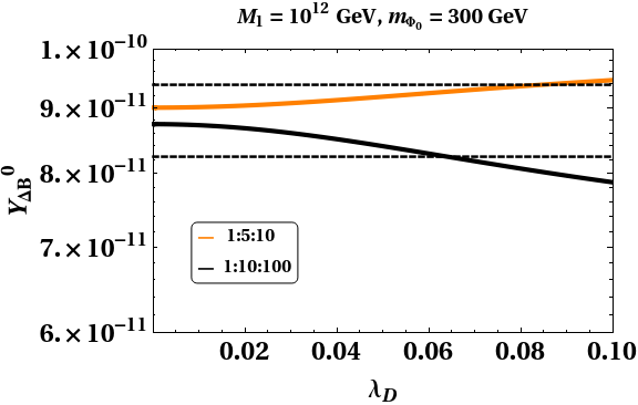
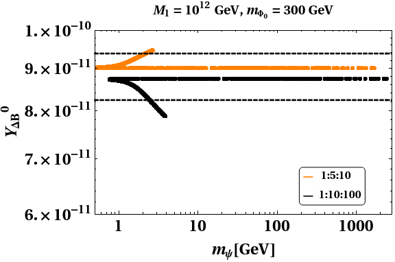
Figure 8: (a)Variation of asymptotic yield $Y_{\Delta B}^{0}$ with dark sector Yukawa coupling $\lambda_{D}$ for $\Delta M=20$ GeV (b) $Y_{\Delta B}^{0}$ vs $m_{\Psi}$ plot satisfying DM relic abundance. In both the plots the variation is shown with two different RHN mass ratios $i.e.$ 1:5:10 and 1:10:100

We now investigate how $Y_{\Delta L,\Delta\Psi}^{0}$ change with RHN mass ratio $i.e.~{}M_{1}:M_{2}:M_{3}$. We first find the $Y$ matrix for a fixed choice of $\Delta M=20$ GeV while considering $M_{1}:M_{2}:M_{3}=1:5:10$ keeping other parameters fixed as in Eq. (45). Then solve the Boltzmann equations (Eqs. (28-29) and results are shown in Fig. 8(a) (Fig. 8(b)) which are similar to Fig. 6(a) (Fig. 7(b)) where we also include the results for earlier mass ratio ($M_{1}:M_{2}:M_{3}=1:10:100$) for comparison purpose. Study of Boltzmann equations indicate that similar to the earlier observations made in Fig. 6(a), here also the first term of Eq. (29) corresponding to $\epsilon_{L}$ dominates over the washout term for visible sector. Whereas, variation of $m_{\Psi}$ with $Y_{\Delta B}^{0}$ in Fig. 8(b) directly reflects from Fig. 8(a). Since $Y_{\Delta B}^{0}$ increases (decreases) with $\lambda_{D}$ for $M_{1}:M_{2}:M_{3}=1:5:10$ ($M_{1}:M_{2}:M_{3}=1:10:100$), behaviour of $m_{\Psi}$ versus $Y_{\Delta B}^{0}$ plots in Fig. 8(b) are different. The parabolic nature of plots in Fig. 8(b) clearly refers to presence strong washout in dark sector as emphasized in earlier discussions. In both the cases of RHN mass ratio considered, observed ADM mass ranges from few GeV to TeV, similar to the ones shown in Fig. 7(b).

VII.2 Study with Inverted Hierarchy

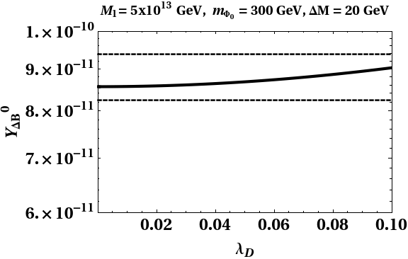
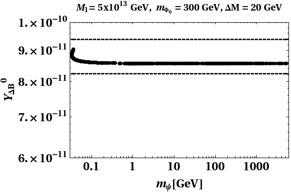
Figure 9: (a)Variation of asymptotic yield $Y_{\Delta B}^{0}$ with dark sector Yukawa coupling $\lambda_{D}$ for $\Delta M=20$ GeV (b) $Y_{\Delta B}^{0}$ vs $m_{\Psi}$ plot satisfying DM relic abundance for the inverted hierarchy.

So far, in Figs. 6 - 8, we have performed our calculations of lepton and dark sector asymmetry assuming normal hierarchy of neutrino mass. In this section, we repeat the study for IH case. Considering the value of $z_{R}=0.78$, $z_{I}=-0.13$, $\Delta M=20$ GeV$,M_{1}=10^{13}$ GeV with rest of the parameters kept fixed as stated while discussing the NH case, $\lambda_{D}$ versus $Y_{\Delta B}^{0}$ ($m_{\Psi}$ versus $Y_{\Delta B}^{0}$) plots are generated in Fig. 9(a) (Fig.9(b)) by solving Boltzmann equations. We do not notice any significant change in the plots of Fig. 9(a)-(b) when compared with NH case and find that for the specific range of $\lambda_{D}$, ADM mass $m_{\Psi}$ goes beyond GeV (to TeV as shown in the present figure). In this regime of $m_{\Psi}$ (from GeV to TeV), the one to one correspondence between $m_{\Psi}$ and $Y_{\Delta B}^{0}$ via $\lambda_{D}$ is lost as observed in case of normal hierarchy too. Such a feature is reminiscent of the combined effect of production and washout of asymmetry being a function of $\lambda_{D}$.

VII.3 Limits from experimental searches

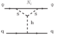
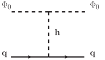
Figure 10: Left panel: Loop suppressed interactions of the dark matter ($\Psi$) with quarks (nucleons) for direct search experiments. Right panel: Direct detection of IHD candidate $\Phi_{0}$.

In this section, we briefly discuss the direct detection limits for the dark matter candidate as well as experimental bounds from LFV and Higgs signal strength. Since we consider $m_{\Phi^{+}}=m_{A_{0}}$, oblique parameter do not impose any constraint in the model and $\Delta T=0$ (see Eq. (11)). Direct detection diagram of asymmetric dark matter $\Psi$ and sub-dominant component $\Phi_{0}$ are shown in Fig. 10. In the present model of asymmetric dark matter, although the dark matter candidate $\Psi$ does not couple directly to the Standard Model Higgs boson or the gauge boson ($Z$), but it acquires an effective vertex $h\Psi\Psi$ at one loop. Hence, the primary scattering interaction for direct interaction is highly suppressed. Therefore, in the present framework, the asymmetric dark matter evades all the direct detection bounds. In a similar manner, one can calculate the direct detection of symmetric dark matter component $\Phi_{0}$. The expression for spin independent direct detection cross-section for $\Phi_{0}$ is expressed as

$$\sigma_{\rm{\Phi_{0}}}^{\rm{SI}}=\frac{\lambda_{L}^{2}}{16\pi}\frac{1}{m_{h}^{4}}f^{2}\frac{m_{N}^{4}}{(m_{\Phi_{0}}+m_{N})^{2}}\,,$$ (47)

where $m_{N}$ denotes the mass of the nucleon and $f\sim 0.32$ Giedt et al. (2009) is Higg-nucleon coupling. It is to be noted that in presence of multi-particle nature (recall that $\Phi_{0}$ contributes 3-6 $\%$ to the relic only), the effective cross-section of $\Phi_{0}$ becomes: $[\frac{\Omega_{\Phi_{0}}h^{2}}{\Omega_{\rm DM}h^{2}}]\sigma_{\rm{\Phi_{0}}}^{\rm{SI}}$. Due to the suppression factor arising out of the ratio ($\frac{\Omega_{\Phi_{0}}h^{2}}{\Omega_{\rm DM}h^{2}}$), it satisfies direct detection bounds Borah et al. (2019); Bhattacharya et al. (2020a, b); Dutta Banik et al. (2020) from XENON1T, LUX.

$M_{1}~{}\rm{[GeV]}$	$m_{\Phi_{0}}~{}\rm{[GeV]}$	$\Delta M~{}\rm{[GeV]}$	$\sigma_{\Phi_{0}}^{eff}($pb$)$	$Br(\mu\rightarrow e\gamma)$	$\mu_{\gamma\gamma}$
$10^{12}$	$300$	$20$	$2.3\times 10^{-12}$	$4.1\times 10^{-54}$	$0.0987$

Table 4: Benchmark values allowed by the direct detection experiments (for $\Phi_{0}$) , $Br(\mu\rightarrow e\gamma)$, Higgs signal strength ($\mu_{\gamma\gamma}$).

In order to discuss the predictions for certain observables in the present set-up, like LFV decays and Higgs signal strength ($\mu_{\gamma\gamma}$), we select a benchmark set of values of parameters for $M_{1},m_{\Phi_{0}}$ and $\Delta M$ as shown in Table 4. Then corresponding to this set of parameters, we provide values for effective direct detection cross-section of $\Phi_{0}$, $\mu_{\gamma\gamma}$ and $Br(\mu\rightarrow e\gamma)$ in the same table which satisfy all the constraints. We calculate the values of $\mu_{\gamma\gamma}$ and ($Br(\mu\rightarrow e\gamma)$) using Eq. (12) (Eq. (17)). We found that the quantity $Br(\mu\rightarrow e\gamma)$ comes out to be many orders of magnitude smaller ($\mathcal{O}(10^{-54})$) (see Table 4) than that of the present experimental bound ($\mathcal{O}(4.1\times 10^{-13})$) as the ratio $\frac{M_{N_{k}}^{2}}{m_{\Phi^{\pm}}^{2}}$ is very large ($\mathcal{O}(10^{20})$ GeV) Toma and Vicente (2014). From Table 4, we conclude that the present asymmetric dark matter model is in agreement with the observed experimental bounds mentioned in Sec. III.

VIII Conclusion

In this framework, we explore a possibility of having a common origin of the dark matter, leptogenesis and neutrino mass by incorporating an inert Higgs doublet ($\Phi$), three right handed neutrinos ($N_{i}$) and a dark sector consisting of a singlet scalar ($S$) and a singlet fermion ($\Psi$). While the interaction of the RHNs with the IHD is responsible for generating the neutrino mass at one loop, its simultaneous decay to the visible (SM leptons and the IHD) and the dark sectors (singlet fermion and scalar) generates asymmetries in both the sectors. A fraction of lepton asymmetry is converted to baryon asymmetry via Sphaleron transition while the asymmetric component of $\Psi$ survives and accounts for the dark matter relic. We particularly focus on the intermediate mass range of the IHD, $i.e.~{}80-500$ GeV as in this regime, its contribution to the relic density of the DM remains sub-dominant and can further be reduced by increasing the mass splitting ($\Delta M$) among its components. In such a scenario where the IHD contributes negligibly to the relic density of the DM, we show that the asymmetric dark matter component of $\Psi$ can provide an explanation for the present day DM abundance of the Universe.

The fate of the present framework at high scale is also tested by doing the RG evolution of all the couplings involved. One finds that the mass splitting, $\Delta M$ of IHD, plays a non trivial role in constraining the allowed parameter space form the high scale validity of the model and at the same time it also restricts the parameter space which explains the present day baryon asymmetry and the DM abundance of the Universe. We show that the $\Delta M\sim\mathcal{O}$(20 GeV) can make the EW vacuum stable while keeping the quartic couplings perturbative till the Planck scale. It turns out that with $\Delta M\sim\mathcal{O}$(20 GeV) there exists a small, but non-zero contribution to the relic density of DM from IHD, making the current framework effectively a two-component dark matter scenario.

We show in the present model that the asymmetries generated in the visible sector can provide an explanation for observed baryon asymmetry of the Universe via leptogenesis whereas the asymmetry generated in the dark sector is responsible for the present DM abundance of the Universe. We perform our analysis for both the normal and the inverted hierarchy of the light neutrino masses. For both NH and IH scenario, the present setup provide a large range of the asymmetric dark matter mass, $m_{\Psi}$ from few GeV to TeV which remains consistent with the correct dark matter abundance of the Universe. We also discuss possible constraints on the model from charged lepton flavor violating decay like $\mu\rightarrow e\gamma$ arising from Yukawa interactions of the RHNs with IHD responsible for neutrino mass generation at one loop. We show that with the chosen set of model parameter $Br(\mu\rightarrow e\gamma)$ comes out to be many orders of magnitude smaller than that of the present experimental bound. We also find that the present model is consistent with various experimental observables such as Higgs signal strength ($\mu_{\gamma\gamma}$) and oblique parameters along with direct and indirect search constraints on IHD. In the present context the RHNs being heavy $\sim\mathcal{O}(10^{12})$ GeV, the effects of flavour in Boltzmann equations have been neglected. However, for the detailed study of leptogenesis with smaller values of RHN mass for which washout effects are significant and hence flavour effects can be relevant. This is expected to be pursued in a different work.

Acknowledgments : Work of ADB and AS was initially supported by Department of Science and Technology, Government of India, under PDF/2016/002148. Work of ADB is also supported in part by National Science Foundation of China (11422545, 11947235). RR would like to thank Arghyajit Datta and Devabrat Mahanta for various useful discussions during the course of this work.

Appendix A 1-loop $\beta-$functions

Below we provide the 1-loop $\beta$-functions for all the couplings involved in the present setup. While generating the $\beta-$functions we have considered one IHD, one scalar singlet, 3 RHNs and a singlet Dirac fermion together with the SM particle spectrum. Since the new particles do not carry any colour charges and the Yukawa interactions of these particles with the SM Higgs are forbidden due to the symmetry assignment of the setup, no modification is observed in the $\beta-$function of the strong coupling $g_{3}$ and the top Yukawa coupling $y_{t}$. The hypercharge for all the BSM fields apart from the IHD is zero , whereas IHD being doublet, also carries a $SU(2)$ charge, this increase in the number of particles carrying a hyper charge and the $SU(2)$ charge leads to modification in the $\beta-$function of $g_{1}$ and $g_{2}$ in comparison to that of the $\beta^{\rm{SM}}_{g_{2}}$ and $\beta^{\rm{SM}}_{g_{2}}$.

A.0.1 SM Couplings

$$\beta_{g_{1}} =\beta_{g_{1}}^{\rm{SM}}+\beta_{g_{1}}^{\rm{IHD}}~{}=~{}\beta_{g_{1}}^{\rm{SM}}+\frac{g_{1}^{3}}{10}$$ (48)

$$\beta_{g_{2}} =\beta_{g_{2}}^{\rm{SM}}+\beta_{g_{2}}^{\rm{IHD}}~{}=~{}\beta_{g_{2}}^{\rm{SM}}+\frac{g_{2}^{3}}{6}$$ (49)

$$\beta_{g_{3}} =\beta_{g_{3}}^{\rm{SM}}$$ (50)

$$\beta_{y_{t}} =\beta_{y_{t}}^{\rm{SM}}$$ (51)

$$\beta_{\lambda_{H}} =\beta_{\lambda_{H}}^{\rm{SM}}+\beta_{\lambda_{H}}^{\rm{IHD}}+\beta_{\lambda_{H}}^{\rm{S}}~{}=~{}\beta_{\lambda_{H}}^{\rm{SM}}+2\lambda_{1}^{2}+2\lambda_{1}\lambda_{2}+\lambda_{2}^{2}+\lambda_{3}^{2}+\frac{1}{2}\lambda^{2}_{HS}$$ (52)

A.0.2 BSM couplings

$$\beta_{\lambda_{S}} =3\Big{(}4\lambda_{HS}^{2}+4\lambda_{\Phi S}^{2}+\lambda_{S}^{2}\Big{)}-48\lambda_{D}^{4}+8\lambda_{S}\lambda_{D}^{2}$$ (53)

$$\beta_{\lambda_{HS}} =-\frac{9}{10}g_{1}^{2}\lambda_{HS}-\frac{9}{2}g_{2}^{2}\lambda_{HS}+4\lambda_{HS}^{2}+4\lambda_{1}\lambda_{\Phi S}+2\lambda_{2}\lambda_{\Phi S}+\lambda_{HS}\lambda_{S}+12\lambda_{HS}\lambda+4\lambda_{HS}\lambda_{D}^{2}$$

$$+6\lambda_{HS}~{}y_{t}^{2}$$ (54)

$$\beta_{\lambda_{\Phi S}} =+4\lambda_{1}\lambda_{HS}+2\lambda_{2}\lambda_{HS}-\frac{9}{10}g_{1}^{2}\lambda_{\Phi S}-\frac{9}{2}g_{2}^{2}\lambda_{\Phi S}+12\lambda_{\Phi}\lambda_{\Phi S}+4\lambda_{\Phi S}^{2}+\lambda_{\Phi S}\lambda_{S}+4\lambda_{\Phi S}\lambda_{D}^{2}$$

$$-8\lambda_{D}^{2}Y^{\dagger}Y+2\lambda_{\Phi S}\mbox{Tr}\Big{(}{YY^{\dagger}}\Big{)}$$ (55)

$$\beta_{\lambda_{\Phi}} =+\frac{27}{200}g_{1}^{4}+\frac{9}{20}g_{1}^{2}g_{2}^{2}+\frac{9}{8}g_{2}^{4}-\frac{9}{5}g_{1}^{2}\lambda_{\Phi}-9g_{2}^{2}\lambda_{\Phi}+24\lambda_{\Phi}^{2}+2\lambda_{1}^{2}+2\lambda_{1}\lambda_{2}+\lambda_{2}^{2}+\lambda_{3}^{2}+\frac{1}{2}\lambda_{\Phi S}^{2}$$

$$+4\lambda_{2}\mbox{Tr}\Big{(}{YY^{\dagger}}\Big{)}-2\mbox{Tr}\Big{(}{YY^{\dagger}YY^{\dagger}}\Big{)}$$ (56)

$$\beta_{\lambda_{1}} =\frac{27}{100}g_{1}^{4}-\frac{9}{10}g_{1}^{2}g_{2}^{2}+\frac{9}{4}g_{2}^{4}-\frac{9}{5}g_{1}^{2}\lambda_{1}-9g_{2}^{2}\lambda_{1}+12\lambda_{\Phi}\lambda_{1}+4\lambda_{1}^{2}+4\lambda_{\Phi}\lambda_{2}+2\lambda_{2}^{2}+2\lambda_{3}^{2}$$

$$+\lambda_{HS}\lambda_{\phi S}+12\lambda_{1}\lambda_{H}+4\lambda_{2}\lambda_{H}+6\lambda_{1}y_{t}^{2}+2\lambda_{1}\mbox{Tr}\Big{(}{YY^{\dagger}}\Big{)}$$ (57)

$$\beta_{\lambda_{2}} =\frac{9}{5}g_{1}^{2}g_{2}^{2}-\frac{9}{5}g_{1}^{2}\lambda_{2}-9g_{2}^{2}\lambda_{2}+4\lambda_{\Phi}\lambda_{2}+8\lambda_{1}\lambda_{2}+4\lambda_{2}^{2}+8\lambda_{3}^{2}+4\lambda_{2}\lambda_{H}+6\lambda_{2}y_{t}^{2}+2\lambda_{2}\mbox{Tr}\Big{(}{YY^{\dagger}}\Big{)}$$ (58)

$$\beta_{\lambda_{3}} =-\frac{9}{5}g_{1}^{2}\lambda_{3}-9g_{2}^{2}\lambda_{3}+4\lambda_{\Phi}\lambda_{3}+8\lambda_{1}\lambda_{3}+12\lambda_{2}\lambda_{3}+4\lambda_{3}\lambda_{H}+6\lambda_{3}y_{t}^{2}+2\lambda_{3}\mbox{Tr}\Big{(}{YY^{\dagger}}\Big{)}$$ (59)

$$\beta_{Y} =\frac{1}{20}\Big{(}10\Big{(}3{YY^{\dagger}Y}+\lambda_{D}^{2}Y+Y\Big{(}20\mbox{Tr}\Big{(}{YY^{\dagger}}\Big{)}-9\Big{(}5g_{2}^{2}+g_{1}^{2}\Big{)}\Big{)}\Big{)}$$ (60)

$$\beta_{\lambda_{D}} =5\lambda_{D}^{3}+Y^{T}Y\lambda_{D}$$ (61)

References

- Fukuda et al. (1998) Y. Fukuda et al. (Super-Kamiokande), Phys. Rev. Lett. 81, 1562 (1998), eprint hep-ex/9807003.
- Ahmad et al. (2002) Q. Ahmad et al. (SNO), Phys. Rev. Lett. 89, 011301 (2002), eprint nucl-ex/0204008.
- Hsu (2006) L. Hsu, Nucl. Phys. B Proc. Suppl. 155, 158 (2006).
- Ahn et al. (2003) M. Ahn et al. (K2K), Phys. Rev. Lett. 90, 041801 (2003), eprint hep-ex/0212007.
- Julian (1967) W. H. Julian, Astrophys. J. 148, 175 (1967).
- Tegmark et al. (2004) M. Tegmark et al. (SDSS), Phys. Rev. D 69, 103501 (2004), eprint astro-ph/0310723.
- Riotto and Trodden (1999) A. Riotto and M. Trodden, Ann. Rev. Nucl. Part. Sci. 49, 35 (1999), eprint hep-ph/9901362.
- Dine and Kusenko (2003) M. Dine and A. Kusenko, Rev. Mod. Phys. 76, 1 (2003), eprint hep-ph/0303065.
- Asaka et al. (2005) T. Asaka, S. Blanchet, and M. Shaposhnikov, Phys. Lett. B 631, 151 (2005), eprint hep-ph/0503065.
- Asaka and Shaposhnikov (2005) T. Asaka and M. Shaposhnikov, Phys. Lett. B 620, 17 (2005), eprint hep-ph/0505013.
- Ma (2006) E. Ma, Phys. Rev. D 73, 077301 (2006), eprint hep-ph/0601225.
- Fukugita and Yanagida (1986) M. Fukugita and T. Yanagida, Phys. Lett. B 174, 45 (1986).
- Buchmuller et al. (2005a) W. Buchmuller, P. Di Bari, and M. Plumacher, Annals Phys. 315, 305 (2005a), eprint hep-ph/0401240.
- Anisimov et al. (2008) A. Anisimov, S. Blanchet, and P. Di Bari, JCAP 04, 033 (2008), eprint 0707.3024.
- Davidson et al. (2008) S. Davidson, E. Nardi, and Y. Nir, Phys. Rept. 466, 105 (2008), eprint 0802.2962.
- Baek et al. (2013) S. Baek, P. Ko, and W.-I. Park, JHEP 07, 013 (2013), eprint 1303.4280.
- Buchmuller et al. (2005b) W. Buchmuller, R. Peccei, and T. Yanagida, Ann. Rev. Nucl. Part. Sci. 55, 311 (2005b), eprint hep-ph/0502169.
- Davoudiasl and Zhang (2015) H. Davoudiasl and Y. Zhang, Phys. Rev. D 92, 016005 (2015), eprint 1504.07244.
- Guo et al. (2017) H.-K. Guo, Y.-Y. Li, T. Liu, M. Ramsey-Musolf, and J. Shu, Phys. Rev. D 96, 115034 (2017), eprint 1609.09849.
- Hernández et al. (2016) P. Hernández, M. Kekic, J. López-Pavón, J. Racker, and J. Salvado, JHEP 08, 157 (2016), eprint 1606.06719.
- Narendra et al. (2018a) N. Narendra, N. Sahoo, and N. Sahu, Nucl. Phys. B 936, 76 (2018a), eprint 1712.02960.
- Dolan et al. (2018) M. J. Dolan, T. P. Dutka, and R. R. Volkas, JCAP 06, 012 (2018), eprint 1802.08373.
- Ipek et al. (2018) S. Ipek, A. D. Plascencia, and J. Turner, JHEP 12, 111 (2018), eprint 1806.00460.
- Das et al. (2020a) P. Das, M. K. Das, and N. Khan, JHEP 03, 018 (2020a), eprint 1911.07243.
- Domcke et al. (2020) V. Domcke, M. Drewes, M. Hufnagel, and M. Lucente (2020), eprint 2009.11678.
- Das et al. (2020b) P. Das, M. K. Das, and N. Khan (2020b), eprint 2010.13084.
- Chen et al. (2020) S.-L. Chen, A. Dutta Banik, and Z.-K. Liu, JCAP 03, 009 (2020), eprint 1912.07185.
- Kashiwase and Suematsu (2012) S. Kashiwase and D. Suematsu, Phys. Rev. D 86, 053001 (2012), eprint 1207.2594.
- Pilaftsis (1997) A. Pilaftsis, Phys. Rev. D 56, 5431 (1997), eprint hep-ph/9707235.
- Pilaftsis and Underwood (2004) A. Pilaftsis and T. E. Underwood, Nucl. Phys. B 692, 303 (2004), eprint hep-ph/0309342.
- Dev et al. (2018a) B. Dev, M. Garny, J. Klaric, P. Millington, and D. Teresi, Int. J. Mod. Phys. A 33, 1842003 (2018a), eprint 1711.02863.
- Barbieri et al. (2006) R. Barbieri, L. J. Hall, and V. S. Rychkov, Phys. Rev. D 74, 015007 (2006), eprint hep-ph/0603188.
- Cirelli et al. (2006) M. Cirelli, N. Fornengo, and A. Strumia, Nucl. Phys. B 753, 178 (2006), eprint hep-ph/0512090.
- Lopez Honorez et al. (2007) L. Lopez Honorez, E. Nezri, J. F. Oliver, and M. H. Tytgat, JCAP 02, 028 (2007), eprint hep-ph/0612275.
- Cao et al. (2007) Q.-H. Cao, E. Ma, and G. Rajasekaran, Phys. Rev. D 76, 095011 (2007), eprint 0708.2939.
- Majumdar and Ghosal (2008) D. Majumdar and A. Ghosal, Mod. Phys. Lett. A 23, 2011 (2008), eprint hep-ph/0607067.
- Lundstrom et al. (2009) E. Lundstrom, M. Gustafsson, and J. Edsjo, Phys. Rev. D 79, 035013 (2009), eprint 0810.3924.
- Dolle and Su (2009) E. M. Dolle and S. Su, Phys. Rev. D 80, 055012 (2009), eprint 0906.1609.
- Lopez Honorez and Yaguna (2010) L. Lopez Honorez and C. E. Yaguna, JHEP 09, 046 (2010), eprint 1003.3125.
- Lopez Honorez and Yaguna (2011) L. Lopez Honorez and C. E. Yaguna, JCAP 01, 002 (2011), eprint 1011.1411.
- Chowdhury et al. (2012) T. A. Chowdhury, M. Nemevsek, G. Senjanovic, and Y. Zhang, JCAP 02, 029 (2012), eprint 1110.5334.
- Arhrib et al. (2014) A. Arhrib, Y.-L. S. Tsai, Q. Yuan, and T.-C. Yuan, JCAP 06, 030 (2014), eprint 1310.0358.
- Plascencia (2015) A. D. Plascencia, JHEP 09, 026 (2015), eprint 1507.04996.
- Borah and Gupta (2017) D. Borah and A. Gupta, Phys. Rev. D 96, 115012 (2017), eprint 1706.05034.
- Biswas and Shaw (2017) A. Biswas and A. Shaw (2017), [Erratum: JCAP 07, E01 (2019)], eprint 1709.01099.
- Falkowski et al. (2011) A. Falkowski, J. T. Ruderman, and T. Volansky, JHEP 05, 106 (2011), eprint 1101.4936.
- Kaplan et al. (2009) D. E. Kaplan, M. A. Luty, and K. M. Zurek, Phys. Rev. D 79, 115016 (2009), eprint 0901.4117.
- Zurek (2014) K. M. Zurek, Phys. Rept. 537, 91 (2014), eprint 1308.0338.
- Hamze et al. (2015) A. Hamze, C. Kilic, J. Koeller, C. Trendafilova, and J.-H. Yu, Phys. Rev. D 91, 035009 (2015), eprint 1410.3030.
- Kitabayashi and Kurosawa (2016) T. Kitabayashi and Y. Kurosawa, Phys. Rev. D 93, 033002 (2016), eprint 1509.05564.
- Frandsen and Shoemaker (2016) M. T. Frandsen and I. M. Shoemaker, JCAP 05, 064 (2016), eprint 1603.09354.
- Murase and Shoemaker (2016) K. Murase and I. M. Shoemaker, Phys. Rev. D 94, 063512 (2016), eprint 1606.03087.
- Agrawal et al. (2017) P. Agrawal, C. Kilic, S. Swaminathan, and C. Trendafilova, Phys. Rev. D 95, 015031 (2017), eprint 1608.04745.
- Nagata et al. (2017) N. Nagata, K. A. Olive, and J. Zheng, JCAP 02, 016 (2017), eprint 1611.04693.
- Baldes and Petraki (2017) I. Baldes and K. Petraki, JCAP 09, 028 (2017), eprint 1703.00478.
- Gresham et al. (2018a) M. I. Gresham, H. K. Lou, and K. M. Zurek, Phys. Rev. D 97, 036003 (2018a), eprint 1707.02316.
- HajiSadeghi et al. (2019) S. HajiSadeghi, S. Smolenski, and J. Wudka, Phys. Rev. D 99, 023514 (2019), eprint 1709.00436.
- Tsao (2018) K.-H. Tsao, J. Phys. G 45, 075001 (2018), eprint 1710.06572.
- Gresham et al. (2018b) M. I. Gresham, H. K. Lou, and K. M. Zurek, Phys. Rev. D 98, 096001 (2018b), eprint 1805.04512.
- Narendra et al. (2018b) N. Narendra, S. Patra, N. Sahu, and S. Shil, Phys. Rev. D 98, 095016 (2018b), eprint 1805.04860.
- Ibe et al. (2018) M. Ibe, A. Kamada, S. Kobayashi, and W. Nakano, JHEP 11, 203 (2018), eprint 1805.06876.
- Van Dong et al. (2019) P. Van Dong, D. Huong, D. A. Camargo, F. S. Queiroz, and J. W. Valle, Phys. Rev. D 99, 055040 (2019), eprint 1805.08251.
- Narendra et al. (2019a) N. Narendra, N. Sahu, and S. Shil (2019a), eprint 1910.12762.
- An et al. (2010) H. An, S.-L. Chen, R. N. Mohapatra, and Y. Zhang, JHEP 03, 124 (2010), eprint 0911.4463.
- Arina and Sahu (2012) C. Arina and N. Sahu, Nucl. Phys. B 854, 666 (2012), eprint 1108.3967.
- Josse-Michaux and Molinaro (2011) F.-X. Josse-Michaux and E. Molinaro, Phys. Rev. D 84, 125021 (2011), eprint 1108.0482.
- Arina (2014) C. Arina, J. Phys. Conf. Ser. 485, 012039 (2014), eprint 1209.1288.
- Gu (2017) P.-H. Gu, JHEP 04, 159 (2017), eprint 1611.03256.
- Fornal et al. (2017) B. Fornal, Y. Shirman, T. M. P. Tait, and J. R. West, Phys. Rev. D 96, 035001 (2017), eprint 1703.00199.
- Yang (2019) W.-M. Yang, Nucl. Phys. B, 114643 (2019), eprint 1807.03036.
- Biswas et al. (2019) A. Biswas, S. Choubey, L. Covi, and S. Khan, JHEP 05, 193 (2019), eprint 1812.06122.
- Narendra et al. (2019b) N. Narendra, S. Patra, N. Sahu, and S. Shil, Springer Proc. Phys. 234, 335 (2019b).
- Ghosh et al. (2018) P. Ghosh, A. K. Saha, and A. Sil, Phys. Rev. D 97, 075034 (2018), eprint 1706.04931.
- Bhattacharya et al. (2020a) S. Bhattacharya, P. Ghosh, A. K. Saha, and A. Sil, JHEP 03, 090 (2020a), eprint 1905.12583.
- Jangid et al. (2020) S. Jangid, P. Bandyopadhyay, P. Bhupal Dev, and A. Kumar, JHEP 08, 154 (2020), eprint 2001.01764.
- Isidori et al. (2001) G. Isidori, G. Ridolfi, and A. Strumia, Nucl. Phys. B609, 387 (2001), eprint hep-ph/0104016.
- Greenwood et al. (2009) E. Greenwood, E. Halstead, R. Poltis, and D. Stojkovic, Phys. Rev. D 79, 103003 (2009), eprint 0810.5343.
- Ellis et al. (2009) J. Ellis, J. R. Espinosa, G. F. Giudice, A. Hoecker, and A. Riotto, Phys. Lett. B679, 369 (2009), eprint 0906.0954.
- Elias-Miro et al. (2012) J. Elias-Miro, J. R. Espinosa, G. F. Giudice, G. Isidori, A. Riotto, and A. Strumia, Phys. Lett. B709, 222 (2012), eprint 1112.3022.
- Alekhin et al. (2012) S. Alekhin, A. Djouadi, and S. Moch, Phys. Lett. B716, 214 (2012), eprint 1207.0980.
- Degrassi et al. (2012) G. Degrassi, S. Di Vita, J. Elias-Miro, J. R. Espinosa, G. F. Giudice, G. Isidori, and A. Strumia, JHEP 08, 098 (2012), eprint 1205.6497.
- Buttazzo et al. (2013) D. Buttazzo, G. Degrassi, P. P. Giardino, G. F. Giudice, F. Sala, A. Salvio, and A. Strumia, JHEP 12, 089 (2013), eprint 1307.3536.
- Anchordoqui et al. (2013) L. A. Anchordoqui, I. Antoniadis, H. Goldberg, X. Huang, D. Lust, T. R. Taylor, and B. Vlcek, JHEP 02, 074 (2013), eprint 1208.2821.
- Tang (2013) Y. Tang, Mod. Phys. Lett. A28, 1330002 (2013), eprint 1301.5812.
- Salvio (2015) A. Salvio, Phys. Lett. B 743, 428 (2015), eprint 1501.03781.
- Salvio (2019) A. Salvio, Phys. Rev. D 99, 015037 (2019), eprint 1810.00792.
- Dutta Banik et al. (2018) A. Dutta Banik, A. K. Saha, and A. Sil, Phys. Rev. D 98, 075013 (2018), eprint 1806.08080.
- Bhattacharya et al. (2020b) S. Bhattacharya, N. Chakrabarty, R. Roshan, and A. Sil, JCAP 04, 013 (2020b), eprint 1910.00612.
- Borah et al. (2020) D. Borah, R. Roshan, and A. Sil, Phys. Rev. D 102, 075034 (2020), eprint 2007.14904.
- Jangid and Bandyopadhyay (2020) S. Jangid and P. Bandyopadhyay, Eur. Phys. J. C 80, 715 (2020), eprint 2003.11821.
- Bandyopadhyay et al. (2020) P. Bandyopadhyay, S. Jangid, and M. Mitra (2020), eprint 2008.11956.
- Borah et al. (2019) D. Borah, R. Roshan, and A. Sil, Phys. Rev. D 100, 055027 (2019), eprint 1904.04837.
- Dutta Banik et al. (2020) A. Dutta Banik, R. Roshan, and A. Sil (2020), eprint 2009.01262.
- Kannike (2012) K. Kannike, Eur. Phys. J. C 72, 2093 (2012), eprint 1205.3781.
- Chakrabortty et al. (2014) J. Chakrabortty, P. Konar, and T. Mondal, Phys. Rev. D89, 095008 (2014), eprint 1311.5666.
- Peskin and Takeuchi (1992) M. E. Peskin and T. Takeuchi, Phys. Rev. D46, 381 (1992).
- Grimus et al. (2008) W. Grimus, L. Lavoura, O. M. Ogreid, and P. Osland, Nucl. Phys. B801, 81 (2008), eprint 0802.4353.
- Arhrib et al. (2012) A. Arhrib, R. Benbrik, and N. Gaur, Phys. Rev. D85, 095021 (2012), eprint 1201.2644.
- Tanabashi et al. (2018) M. Tanabashi et al. (Particle Data Group), Phys. Rev. D98, 030001 (2018).
- Swiezewska and Krawczyk (2013) B. Swiezewska and M. Krawczyk, Phys. Rev. D88, 035019 (2013), eprint 1212.4100.
- Aaboud et al. (2018) M. Aaboud et al. (ATLAS), Phys. Rev. D98, 052005 (2018), eprint 1802.04146.
- Sirunyan et al. (2018) A. M. Sirunyan et al. (CMS), JHEP 11, 185 (2018), eprint 1804.02716.
- Aghanim et al. (2018) N. Aghanim et al. (Planck) (2018), eprint 1807.06209.
- Akerib et al. (2017) D. Akerib et al. (LUX), Phys. Rev. Lett. 118, 021303 (2017), eprint 1608.07648.
- Aprile et al. (2018) E. Aprile et al. (XENON), Phys. Rev. Lett. 121, 111302 (2018), eprint 1805.12562.
- Tan et al. (2016) A. Tan et al. (PandaX-II), Phys. Rev. Lett. 117, 121303 (2016), eprint 1607.07400.
- Cui et al. (2017) X. Cui et al. (PandaX-II), Phys. Rev. Lett. 119, 181302 (2017), eprint 1708.06917.
- Ma and Raidal (2001) E. Ma and M. Raidal, Phys. Rev. Lett. 87, 011802 (2001), [Erratum: Phys.Rev.Lett. 87, 159901 (2001)], eprint hep-ph/0102255.
- Toma and Vicente (2014) T. Toma and A. Vicente, JHEP 01, 160 (2014), eprint 1312.2840.
- Baek et al. (2014) S. Baek, H. Okada, and T. Toma, Phys. Lett. B 732, 85 (2014), eprint 1401.6921.
- Das et al. (2017) A. Das, T. Nomura, H. Okada, and S. Roy, Phys. Rev. D 96, 075001 (2017), eprint 1704.02078.
- Baldini et al. (2016) A. Baldini et al. (MEG), Eur. Phys. J. C 76, 434 (2016), eprint 1605.05081.
- Ahriche et al. (2018) A. Ahriche, A. Jueid, and S. Nasri, Phys. Rev. D 97, 095012 (2018), eprint 1710.03824.
- Maki et al. (1962) Z. Maki, M. Nakagawa, and S. Sakata, Prog. Theor. Phys. 28, 870 (1962).
- Davidson and Ibarra (2002) S. Davidson and A. Ibarra, Phys. Lett. B 535, 25 (2002), eprint hep-ph/0202239.
- Edsjo and Gondolo (1997) J. Edsjo and P. Gondolo, Phys. Rev. D 56, 1879 (1997), eprint hep-ph/9704361.
- Hugle et al. (2018) T. Hugle, M. Platscher, and K. Schmitz, Phys. Rev. D 98, 023020 (2018), eprint 1804.09660.
- Mahanta and Borah (2019) D. Mahanta and D. Borah, JCAP 11, 021 (2019), eprint 1906.03577.
- Mahanta and Borah (2020) D. Mahanta and D. Borah, JCAP 04, 032 (2020), eprint 1912.09726.
- Casas and Ibarra (2001) J. Casas and A. Ibarra, Nucl. Phys. B 618, 171 (2001), eprint hep-ph/0103065.
- Staub (2014) F. Staub, Comput. Phys. Commun. 185, 1773 (2014), eprint 1309.7223.
- Abada et al. (2006a) A. Abada, S. Davidson, F.-X. Josse-Michaux, M. Losada, and A. Riotto, JCAP 04, 004 (2006a), eprint hep-ph/0601083.
- Nardi et al. (2006) E. Nardi, Y. Nir, E. Roulet, and J. Racker, JHEP 01, 164 (2006), eprint hep-ph/0601084.
- Abada et al. (2006b) A. Abada, S. Davidson, A. Ibarra, F.-X. Josse-Michaux, M. Losada, and A. Riotto, JHEP 09, 010 (2006b), eprint hep-ph/0605281.
- Blanchet and Di Bari (2007) S. Blanchet and P. Di Bari, JCAP 03, 018 (2007), eprint hep-ph/0607330.
- Blanchet et al. (2007) S. Blanchet, P. Di Bari, and G. Raffelt, JCAP 03, 012 (2007), eprint hep-ph/0611337.
- Dev et al. (2018b) P. S. B. Dev, P. Di Bari, B. Garbrecht, S. Lavignac, P. Millington, and D. Teresi, Int. J. Mod. Phys. A 33, 1842001 (2018b), eprint 1711.02861.
- Ade et al. (2016) P. Ade et al. (Planck), Astron. Astrophys. 594, A13 (2016), eprint 1502.01589.
- Giedt et al. (2009) J. Giedt, A. W. Thomas, and R. D. Young, Phys. Rev. Lett. 103, 201802 (2009), eprint 0907.4177.