SuperDeConFuse: A Supervised Deep Convolutional Transform based Fusion Framework for Financial Trading Systems

Pooja Gupta
Indraprastha Institute of Information Technology, Delhi, India
poojag@iiitd.ac.in
Angshul Majumdar
Indraprastha Institute of Information Technology, Delhi, India
angshul@iiitd.ac.in
Emilie Chouzenoux
CVN, Inria Saclay, CentraleSupélec, Gif-sur-Yvette, France
emilie.chouzenoux@centralesupelec.fr
Giovanni Chierchia
LIGM, Université Gustave Eiffel, CNRS, ESIEE Paris, Noisy-le-Grand, France
giovanni.chierchia@esiee.fr

Abstract

This work proposes a supervised multi-channel time-series learning framework for financial stock trading. Although many deep learning models have recently been proposed in this domain, most of them treat the stock trading time-series data as 2-D image data, whereas its true nature is 1-D time-series data. Since the stock trading systems are multi-channel data, many existing techniques treating them as 1-D time-series data are not suggestive of any technique to effectively fusion the information carried by the multiple channels. To contribute towards both of these shortcomings, we propose an end-to-end supervised learning framework inspired by the previously established (unsupervised) convolution transform learning framework. Our approach consists of processing the data channels through separate 1-D convolution layers, then fusing the outputs with a series of fully-connected layers, and finally applying a softmax classification layer. The peculiarity of our framework, that we call SuperDeConFuse (SDCF), is that we remove the nonlinear activation located between the multi-channel convolution layers and the fully-connected layers, as well as the one located between the latter and the output layer. We compensate for this removal by introducing a suitable regularization on the aforementioned layer outputs and filters during the training phase. Specifically, we apply a logarithm determinant regularization on the layer filters to break symmetry and force diversity in the learnt transforms, whereas we enforce the non-negativity constraint on the layer outputs to mitigate the issue of dead neurons. This results in the effective learning of a richer set of features and filters with respect to a standard convolutional neural network. Numerical experiments confirm that the proposed model yields considerably better results than state-of-the-art deep learning techniques for the real-world problem of stock trading.

1 Introduction

Financial time series forecasting, and particularly stock price forecasting, requires to determine the future value of a company’s stock or any other form of a financial instrument traded on exchange as per the company. It plays a significant role in trading strategies to identify opportunities to buy and sell a stock and this process is known as stock trading. This future movement prediction of stock could capitulate the significant profit.

However, the problem of stock trading has been one of the most difficult problems for the researchers in finance data processing, and speculators. Struggles are mainly due to the uncertainties and noises of the samples. These samples are generated as a consequence of historical market behaviors. But their generation is also affected by other factors such as macroeconomy and investor feelings, hence it is not only dependent on historical information [Sezer & Ozbayogl, 2018]. Two famous hypotheses emphasize how difficult it is to accurately predict a stock price. First, the efficient market hypothesis introduced in [Fama & Malkiel, 1970] states that the current price of an asset always reflects all previous information available for it instantly. Second, the random-walk hypothesis [Malkiel, 1973] claims that stock price changes independently from its history. In other words, tomorrow’s price will only depend on tomorrow’s information regardless of today’s price. Hence, automating the prediction of stock trends/movements is a very challenging task.

In past works, feature engineering played a key role in the prediction process. Features were extracted from the original stock data using technical analysis/indicators, which are in general used for analysing the stock market data. Traditional statistical methods such as linear regression, autoregressive moving average (ARMA), and GARCH, were much beneficial for financial time series forecasting due to their interpretability. These statistical models were thus used on the extracted features, processed using technical indicators related to historical data for future value prediction [Shynkevich et al., 2017]. Previous works have also used the extracted features as input to machine learning models like Naive Bayes (NB), Logistic Regression (LR), Random Forest (RF), and k-nearest neighbors (kNN) [Patel et al., 2015a, Sen & Chaudhuri, 2017, Ballings et al., 2015].

In the last decade, deep learning based models/techniques have gained attention in multiple domains, and financial stock trading is one such domain. Owing to the success of Convolutional Neural Networks (CNNs), there are previous studies that have used this model for the future prediction of the stock value. In [Sezer & Ozbayogl, 2018], the features extracted using technical indicators for stock data are fed as a 2-D “image” matrix to the CNN, where each column represents shifted windows of the data. The work [Long et al., 2019] utilizes long short-term memory (LSTM), deemed most suitable for time series analysis as they were supposed to mimic memory, and CNN for the stock trading task. However, it is likely that the most natural and thus efficient way to process time-series is to consider its original form as 1-D data rather than a 2-D matrix. It is worth mentioning that, up to our knowledge, despite its multi-channel form, the problem of financial stock trading has been rarely treated as a fusion problem. We can only mention [Yang et al., June 2015a, Yao et al., April 2017] where a fusion framework is proposed, but only at the feature level rather than at the raw level.

In this work, motivated by the success of CNNs, we propose an end-to-end supervised fusion framework for multi-channel time-series based financial trading systems that makes use of our recently introduced convolutional transform learning (CTL) approach [Maggu et al., Dec 2018]. We call this framework -SuperDeConFuse (SDCF). Our framework has the following contributions:

• It is an end-to-end framework that treats the multi-channel time-series stock data as univariate data corresponding to every channel, thus overcoming both the aforementioned issues present in the previous works solving the problem of stock trading.

• It promotes the learning of unique filters and hence a richer set of features, that was not guaranteed with CNNs, due to a “logarithm determinant” penalty applied to the transforms/filters.

• A non-negativity constraint on coefficients/features mitigates the dead neurons issue by removing the nonlinear activation of the fully-connected layers and the last convolution layer.

The remainder of this paper is organized as follows. Section 2 summarizes related works in the field of machine learning and deep learning that have been proposed for solving the stock trading problem/ stock market prediction.

Since our work focuses on a supervised multi-channel fusion framework, we will also review recent machine learning approaches for information fusion. Section 3 introduces the details of our proposed SuperDeConFuse (SDCF) approach, the mathematical tools involved and the training strategy that is retained. Section 4 discusses the considered dataset, data labeling, data preprocessing and the training methodology used. Section 5 provides the experimental results. Finally, Section 6 concludes this work.

2 Literature Review

2.1 Financial stock data analysis

In literature, different methodologies have been applied to the stock data for predicting future trading strategies (eg, buy and sell decisions). These include statistical methods, machine learning algorithms like Support Vector Machine (SVM) and Artificial Neural Networks (ANN), feature extraction approaches, deep learning models (eg, CNN, LSTM), that we briefly review in this section.

Statistical methods are probably the methods among others that are universally used for the prediction of financial stock trading strategies. In particular, many studies rely on the use of sequential statistical models, such as ARMA [Kocak, 2017], ARCH [Zumbach & Fernndez, 2014], GARCH [Lin, 2018] and [lk et al., 2017], Kalman filter [Bisoi & Dash, 2014].

Feature-based techniques are also considered as state-of-the-art. Technical indicators like Exponential moving average (EMA), Moving average convergence and divergence (MACD), Williams %R, etc. have been used in past studies to extract the features from the data. Text mining can be used to process financial analysis from newspapers [Ming et al., 2014]. The features are then used as input to machine learning models, for example, SVM, ANN, kNN [Shynkevich et al., 2017]. Another work [Royo & Guijarro, 2019] compares various off-the-shelf machine learning tools for stock prediction. Further studies have proposed hybrid machine learning models, based on the use of multiple types of base classifiers that operate on a common input and a meta classifier that learns from base classifiers’ outputs to obtain a more precise stock return and risk predictions. In the work [Garcia et al., 2018], the authors study the performance of financial technical indicators when used as inputs instead of machine learning based features for a neuro-fuzzy classifier. The study by [Tsinaslanidis & Guijarro, 2020] uses a sophisticated version of template matching called chart pattern recognition to identify profitable stocks. Strategies such as Bagging, Boosting and AdaBoost, can be also applied to create diversity in classifier combinations [Barak et al., 2017, Weng et al., 2018]. For example, a hybrid weighted SVM and weighted KNN model for predicting stock market indices is proposed in [Chen & Hao, 2017]. Similarly, a technique that combines Support Vector Regression (SVR), Random Forests and ANNs for predicting stock market index, is introduced in [Patel et al., 2015b]. Another study [Ticknor, 2013] combines the statistical and probabilistic Bayesian Learning and the machine learning model ANN for the same. However, in all the aforementioned techniques, the relationship built between historical data and future value prediction may lack interpretation because of their “black-box” property and, thus, the performance of these methods are directly related to the quality of the features. Moreover, with machine learning techniques, overfitting is a major issue owing to their capability of non-linear mapping and fitting.

Deep learning based models have also been extensively used for solving stock forecasting problems. Recurrent Neural Networks (RNNs) are considered to be the most appropriate models for time-series analysis. LSTM is one such RNN which is regarded as the memory-mimicking model. Some studies use LSTM for the time-series stock forecasting [Nelson et al., 2017]. Another work uses LSTM on the technical indicators for the prediction [Tingwei & Yueting, 2018]. However, despite the great performance obtained, the time complexity of training RNN via backpropagation has encouraged the users for searching for more tractable models and solutions. CNNs constitute another important deep learning model, apart from RNNs, which have been used profusely and have performed well in the stock time-series forecasting, especially 2-D CNNs. In [Sezer & Ozbayogl, 2018], the said techniques have been used on stock prices for forecasting. A slightly different input is used in [Tsantekidis et al., July 2017], instead of using the standard variables (opening, closing, high, low and NAV), it uses high frequency data for forecasting major points of inflection in the financial market. In another work [Gudelek et al., November 2017], a similar approach is used for modeling exchange traded fund (ETF). The 2-D CNN model performs similarly as LSTM or the standard multi-layer perceptron [Persio & Honchar, 2016, Hiransha et al., 2018] while being simpler to train. This apparent lack of performance improvement may be owing to the incorrect choice of CNN model, since these studies model an inherently 1D time series as an image.

2.2 Information Fusion

Many real world domains raise problems pertaining to the need for the fusion of information from multiple sources. Consider the problem of demand forecasting which requires estimating the power consumption at a future point given the available information until the current instant. At the building level forecasting, the inputs are usually power consumption, weather (temperature, humidity), and occupancy. This is a crucial problem in smart grids that ranges from planning electricity generation to preventing non-technical losses. Another area is biomedical signal analysis, for example, the problem of blood pressure estimation. The inputs are usually from two sources, namely the electrocardiogram (ECG) and pulsepleithismogram (PPG) [Yoon et al., 2009], and the goal is to estimate the systolic and diastolic pressures. Transportation is also one such domain that needs the fusion of information from many sources to build intelligent transportation systems (ITS) [El Faouzi et al., 2011, Saadi et al., 2018]. This is needed to improve passenger safety, reduced transportation time and fuel consumption, etc.

Image fusion is another area where the information from two or more images of an object has to be integrated into a single image that is more informative and appropriate for visual perception or computer analysis. It finds great application in medical imaging. One can mention for instance the fusion of MRI (Magnetic Resonance Imaging) and PET (Positron Emission Tomography) images using IHS (Intensity Hue Saturation) and RIM (Retina-Inspired Models) fusion methods to improve the functional and spatial information content of the PET images [Daneshvar & Ghassemian, 2010].

Deep learning has been widely used for analyzing multi-channel / multi-sensor signals. In such studies, all the sensors are stacked one after the other to form a matrix using 2-D CNN further to analyze these signals. For example, [Yang et al., June 2015b] uses the same explained model to analyze human activity recognition from multiple body sensors. Note that it must be distinguished from the studies mentioned before [Sezer & Ozbayogl, 2018, Tsantekidis et al., July 2017, Gudelek et al., November 2017, Persio & Honchar, 2016, Hiransha et al., 2018], as the images in [Yang et al., June 2015b] are not formed from stacking windowed signals from the same signal one after the other, they are formed by stacking signals from different sensors. Note, however, that [Yang et al., June 2015b] does not account for any temporal modeling. This is rectified in [Yao et al., April 2017] where 2-D CNN is used on a time series window. The different windows are finally processed by GRU, thus explicitly incorporating time series modeling. In the aforesaid studies, there is however no explicit fusion framework. The information from raw signals is fused to form matrices and treated by 2-D convolutions. A true fusion framework was proposed in [Zheng et al., June 2014]. Here, the fusion was happening at the feature level and not in the raw signal level as was in [Yang et al., June 2015b, Yao et al., April 2017].

Multi-modal data processing is another area that makes use of deep learning based fusion techniques. Although this problem is not multi-channel data processing per se, we will briefly review here some studies on this topic. In [Ngiam et al., 2011] a fusion scheme is proposed for audio-visual analysis, that uses a fusion scheme for deep belief network (DBN) and stacked autoencoder (SAE) for fusing the audio and video channels. Each of the said channels is processed separately and connected by a fully connected layer to produce fused features. These fused features are further processed for inference. The problem of video based action recognition is addressed in [Feichtenhofer et al., 2016]. It does not require audio data for the task; rather it proposes a fusion scheme for incorporating temporal information (processed by CNN) and spatial information (also processed by CNN). Experiments were carried out with different levels of early and late fusion. The fusion of multi-channel image dataset has also been investigated. In [Eitel et al., September 2015], a fusion scheme is proposed for processing color and depth information (via 3-D and 2-D convolutions, respectively) with the objective of action recognition. In [Chen et al., 2017], the authors consider fusing hyperspectral data (high spatial resolution) with Lidar (depth information), with the consequence of better classification results. In [Antropova et al., 2017], it was shown that by fusing deeply learnt features (from CNN) with handcrafted features via a fully connected layer, can improve analysis tasks.

It is worthy to point out that the aforementioned time-series data based fusion studies do not process the time-series data as 1-D but as 2-D image/matrix. In the context of financial time-series, the state-of-the-art methods seem mostly based either on statistical and machine learning models or CNNs. For the former, the relationship built between historical data and future value prediction may lack interpretation because of their “black-box” property; and hence, the performance of the methods is directly related to the quality of the features. While in the latter case of CNNs, there is no guarantee of unique filters learnt. In this work, we propose a novel framework that can tackle those issues.

3 Proposed Technique

This paper introduces a novel supervised framework for multi-channel data representation learning. A crucial element of the latter is our recently introduced CTL [Maggu et al., Dec 2018]. For clarity, we first recall the important steps of the CTL technique. Then, we propose an extension of this approach in order to handle a multi-layer architecture. Finally, we present the overall SuperDeConFuse (SDCF) architecture.

3.1 Convolutional Transform Learning

As introduced in our seminal paper [Maggu et al., Dec 2018], CTL learns some filters $\left(t_{m}\right)_{1\leq m\leq M}$ operated on samples $\left(s^{(k)}\right)_{1\leq k\leq K}$ to generate the features $\big{(}x_{m}^{(k)}\big{)}_{1\leq m\leq M,1\leq k\leq K}$. The inherent learning model is expressed by convolution operations (assuming suitable padding) defined as

$$(\forall m\in\{1,\ldots,M\}\;,\forall k\in\{1,\ldots,K\})\qquad{t_{m}}*{s^{(k)}}=x_{m}^{(k)}.$$ (1)

A regularization is imposed on the filters to improve the representation ability and limit the overfitting issues, following from the original study on transform learning [Ravishankar & Bresler, 2012]. Also, non-negativity constraint is imposed on the features, as it is commonly done in CNNs. The convolutional filters and the representation coefficients are learnt from the data during training. This is expressed as the following optimization problem:

$$\underset{\begin{subarray}{c}{{(t_{m})_{m}},(x_{m}^{(k)})_{m,k}}\end{subarray}}{\textrm{minimize}}\;\;\frac{1}{2}\sum\limits_{k=1}^{K}{\sum_{m=1}^{M}\Big{(}{\big{\|}{{t_{m}}*{s^{(k)}}-x_{m}^{(k)}}\big{\|}_{2}^{2}}}+\psi(x_{m}^{(k)})\Big{)}\\ +\mu\sum_{m=1}^{M}\left\|t_{m}\right\|_{2}^{2}-\lambda\log\det\big{(}[{{t_{1}}\;\ldots\;{t_{M}}}]\big{)},$$ (2)

where $\psi$ is a suitable penalization function, and $(\mu,\lambda)$ are positive hyperparameters. It should be noted that the regularization term promotes unique filters to be learnt, something that is not easy to guarantee in CNNs. We can rewrite equivalently Equation (2) in matrix notation as

$$F(T,X)=\frac{1}{2}\left\|T\star S-X\right\|_{F}^{2}+\Psi(X)+\mu\left\|T\right\|_{F}^{2}-\lambda\log\det\left(T\right),$$ (3)

where $T=\begin{bmatrix}t_{1}&\dots&t_{M}\end{bmatrix}$, $S=\begin{bmatrix}s^{(1)}&\dots&s^{(K)}\end{bmatrix}^{\top}$, $X=\begin{bmatrix}x_{1}^{(k)}&\dots&x_{M}^{(k)}\end{bmatrix}_{1\leq k\leq K}$,

$$T\star S=\begin{bmatrix}t_{1}*s^{(1)}&\dots&t_{M}*s^{(1)}\\ \vdots&\ddots&\vdots\\ t_{1}*s^{(K)}&\dots&t_{M}*s^{(K)},\end{bmatrix}$$ (4)

and $\Psi$ amounts to applying the penalty term $\psi$ column-wise on $X$ and summing.

A local minimizer to (3) can be reached efficiently using the alternating proximal algorithm [Attouch et al., Feb 2011, Chouzenoux et al., 2016, Bolte et al., 2014], which alternates between proximal updates on variables $T$ and $X$. The proximity operator [Combettes & Pesquet, 2011] at $\tilde{x}\in\mathcal{H}$, with $(\mathcal{H},\|\cdot\|)$ a Hilbert space, of a proper lower-semi-continuous convex function $\varphi:\mathcal{H}\to]-\infty,+\infty]$ is defined as

$$\operatorname{prox}_{\varphi}(\tilde{x})=\mathop{\arg\min}\limits_{x\in\mathcal{H}}\varphi(x)+\frac{1}{2}\left\|{x-\tilde{x}}\right\|^{2}.$$ (5)

Then, the alternating proximal algorithm for CTL reads:

$$\begin{array}[]{l}{\rm{For\ }}{n}=0,1,...\\ \left\lfloor\begin{array}[]{rl}T^{[n+1]}&=\operatorname{prox}_{\gamma_{1}F(\cdot,X^{[n]})}\left(T^{[n]}\right)\\ X^{[n+1]}&=\operatorname{prox}_{\gamma_{2}F(T^{[n+1]},\cdot)}\left(X^{[n]}\right)\end{array}\right.\end{array}$$ (6)

with initializations $T^{[0]}$, $X^{[0]}$ of suitable dimensions, and ${\gamma_{1}},{\gamma_{2}}$ some positive constants. For more details on the derivations and the convergence guarantees, the readers can refer to [Maggu et al., Dec 2018].

3.2 Deep Convolutional Transform Learning

Deep CTL consists in stacking multiple convolutional layers on top of each other to generate the features, as shown in Figure 1. Deep CTL depends on the key property that the solution $\widehat{X}$ to the CTL problem, assuming fixed filters $T$, can be reformulated as the simple application of an element-wise activation function. That is:

$$\operatorname*{argmin}_{X}F(T,X)=\Phi\big{(}T\star S\big{)},$$ (7)

with $\Phi$ the proximity operator of $\Psi$ [Combettes & Pesquet, 2018]. It is interesting to remark that, if $\Psi$ is the indicator function of the positive orthant, then $\Phi$ identifies with the famous rectified linear unit (ReLU) activation function. Many other examples of mapping between proximity operators and activation functions are provided in [Combettes & Pesquet, 2018]. Consequently, we propose to compute deep features by stacking many such layers:

$$(\forall\ell\in\{1,\dots,L-1\})\qquad X_{\ell}=\Phi_{\ell}(T_{\ell}\star X_{\ell-1}),$$ (8)

where we set $X_{0}=S$. Deep CTL consists of solving the problem

$$\underset{\begin{subarray}{c}{T_{1},\dots,T_{L},X}\end{subarray}}{\textrm{minimize}}\;\;F_{\rm conv}(T_{1},\dots,T_{L},X\,|\,S)$$ (9)

with

$$F_{\rm conv}(T_{1},\dots,T_{L},X\,|\,S) =\frac{1}{2}\|T_{L}\star\Phi_{L-1}(T_{L-1}\star\dots\Phi_{1}(T_{1}\star S))-X\|_{F}^{2}$$

$$+\Psi(X)+\sum_{\ell=1}^{L}\big{(}\mu||T_{\ell}||^{2}_{F}-\lambda\log\det(T_{\ell})\big{)}.$$ (10)

Deep CTL can thus be viewed as a natural and simple extension of the one-layer CTL formulation in (3).

Figure 1: Deep CTL architecture for $L=2$ layers.

3.3 Our Proposed Approach - SuperDeConFuse

We now present our novel approach, SuperDeConFuse (SDCF), which is a supervised fusion framework for multi-channel time-series stock data. This framework takes the channels of input data samples to separate branches of convolutional layers, leading to multiple sets of channel-wise features. The features obtained are thus decoupled. In order to couple (i.e., fuse) them, these are concatenated and passed to a fully-connected layer, which yields a set of unique coupled features via transform learning. These features are then fed to another linear fully-connected layer. This provides features that are finally inputted to the softmax layer that yields the probabilities for the classes. The complete architecture, called SuperDeConFuse (SDCF), is shown in Figure 2.

Figure 2: SuperDeConfuse Architecture. The architecture is tested for $L=1,2,3,4$ layers. Here $P_{1}\times 1,\ldots,P_{L}\times 1$ represents the kernel size used in each layer $\ell\in\{1,\ldots,L\}$. Here, maxpooling is not performed after layer $4$ due to the small window size/input sequence length.

As the data considered is multi-channel, we learn a different set of convolutional filters $T^{(c)}_{1},\ldots,T^{(c)}_{L}$ and features $X^{(c)}$ for each channel $c\in\{1,\ldots,C\}$. We also learn the (not convolutional) linear transform $\widetilde{T}=(\widetilde{T_{c}})_{1\leq c\leq C}$ to fuse the channel-wise features $X=(X^{(c)})_{1\leq c\leq C}$, along with the corresponding fused features $Z$ at the same time. The latter task is carried out by the cost function

$$F_{\rm fusion}(\widetilde{T},Z,X)=\frac{1}{2}\Big{\|}Z-\sum^{C}_{c=1}{\rm flat}(X^{(c)})\widetilde{T}_{c}\Big{\|}^{2}_{F}+\Psi(Z)+\sum_{c=1}^{C}\Big{(}\mu\Big{\|}\widetilde{T_{c}}\Big{\|}^{2}_{F}-\lambda\log\det(\widetilde{T_{c}})\Big{)}$$ (11)

where the operator “$\operatorname{flat}$” transforms $X^{(c)}$ into a matrix where each row contains the “flattened” features of a sample.

Further, we learn the weight matrix $\theta$ of a multiclass classifier which takes the input features $Z$ and yields the class probabilities. The cross-entropy (CE) loss associated with the final classification is given by

$$F_{\textrm{CE}}(\theta,Z\,|\,y)=\sum_{k=1}^{K}\log\Big{(}\sum_{v=1}^{V}e^{z_{k}^{\top}(\theta_{v}-\theta_{y_{k}})}\Big{)},$$ (12)

where $V$ is the number of classes, $\theta_{v}$ is the $v$-th column of matrix $\theta$, $z_{k}^{\top}$ is the $k$-th row of matrix $Z$, and $y_{k}\in\{1,\dots,V\}$ is the label of the $k$-th sample. This finally leads to the joint optimization problem defined as

$$\underset{\begin{subarray}{c}{(T,X,\widetilde{T},Z,\theta)}\end{subarray}}{\textrm{minimize}}\;\;\underbrace{\sum_{c=1}^{C}F_{\rm conv}(T_{1}^{(c)},\ldots,T_{L}^{(c)},X^{(c)}|S^{(c)})+F_{\rm fusion}(\widetilde{T},Z,X)+F_{\rm CE}(\theta,Z\,|\,y).}_{J(T,X,\widetilde{T},Z,\theta)}$$ (13)

Conclusively, our formulation aims at jointly training the channel-wise convolutional filters $T_{l}^{(c)}$, the fusion coefficients $\widetilde{T}$, and the multiclass classifier $\theta$ in an end-to-end fashion. We explicitly learn the features $X$ and $Z$ subject to the regularization $\Psi$, so as to avoid the problem of dead neurons. Moreover, the “log-det” regularization on both $T_{l}^{(c)}$ and $\widetilde{T}$ breaks the symmetry and enforces the diversity in the learnt transforms, whereas the Frobenius regularization keeps the transform coefficients bounded.

3.4 Optimization algorithm

We propose to find a local minimizer to the nonconvex Problem (13) through the projected (sub)gradient descent, whose iterations read:

$$\begin{array}[]{l}{\rm{For\ }}{n}=0,1,...\\ \;\left\lfloor\begin{array}[]{rl}T^{[n+1]}&=T^{[n]}-\gamma\nabla_{T}J(T^{[n]},X^{[n]},\widetilde{T}^{[n]},Z^{[n]},\theta^{[n]})\\ X^{[n+1]}&=\mathcal{P}_{+}\big{(}X^{[n]}-\gamma\nabla_{X}J(T^{[n]},X^{[n]},\widetilde{T}^{[n]},Z^{[n]},\theta^{[n]})\big{)}\\ \widetilde{T}^{[n+1]}&=\widetilde{T}^{[n]}-\gamma\nabla_{\widetilde{T}}J(T^{[n]},X^{[n]},\widetilde{T}^{[n]},Z^{[n]},\theta^{[n]})\\ Z^{[n+1]}&=\mathcal{P}_{+}\big{(}Z^{[n]}-\gamma\nabla_{Z}J(T^{[n]},X^{[n]},\widetilde{T}^{[n]},Z^{[n]},\theta^{[n]})\big{)}\\ \theta^{[n+1]}&=\theta^{[n]}-\gamma\nabla_{\theta}J(T^{[n]},X^{[n]},\widetilde{T}^{[n]},Z^{[n]},\theta^{[n]})\\ \end{array}\right.\end{array}$$ (14)

with $\mathcal{P}_{+}=\max\{\cdot,0\}$ (applied element-wise). In practice, we initialize it with some random matrices $T^{[0]},X^{[0]},\widetilde{T}^{[0]},Z^{[0]},\theta^{[0]}$, we choice a suitable stepsize $\gamma>0$, and we evaluate numerically the gradient step with the accelerated scheme initially introduced for the ADAM method in [Kingma & Ba, 2015].

There are two remarkable advantages of the proposed optimization approach. Firstly, we depend on automatic differentiation [Paszke et al., 2017] and stochastic gradient approximations to efficiently solve Problem (13). Secondly, any sub-differentiable activation function $\Phi$ in (7) can be plugged into our model, for instance SELU [Klambauer et al., 4-9 Dec. 2017] or Leaky ReLU [Mass et al., 2013]. This flexibility will play a key role in the performance, as shown in the experimental section.

3.5 Computational Complexity of Proposed Framework - SuperDeConFuse(SDCF)

Table 1 summarizes the computational complexity of SuperDeconFuse(SDCF) architecture, both for training and test phases. We report the cost incurred for one input sample, either at an iteration of the training algorithm or at the testing phase. It is to be noted that the computational complexity of SDCF architecture is comparable to that of a standard CNN. The log-det regularization is the only addition that requires to compute the truncated singular value decomposition of $T_{\ell}^{(c)}$ and $\widetilde{T}_{c}$. However, as the size of these matrices is determined by the filter size, the number of filters, and the number of output features per sample, the training complexity is not worse than that of a CNN.

Table 1: Time complexity in training and test phases (for one input sample)

Phase	Steps	Time	Dimension
		Complexity	Description
Training	1. Convolution layers	$\mathcal{O}(P_{\ell}D_{\ell}M_{\ell}C)$
	2. Fully-connected (f.-c.) layer	$\mathcal{O}(I^{2}C^{2})$	$S^{(c)}\in\mathbb{R}^{K\times D}$
	3. Frobenius norm on conv. layers	$\mathcal{O}\big{(}P_{\ell}M_{\ell}C\big{)}$	$T_{\ell}^{(c)}\in\mathbb{R}^{P_{\ell}\times M_{\ell}}$
	4. Frobenius norm on f.-c. layer	$\mathcal{O}(I^{2}C^{2})$	${\rm flat}(X^{(c)})\in\mathbb{R}^{K\times I}$
	5. log-det on conv. layers	$\mathcal{O}(P_{\ell}^{2}M_{\ell}C)$	$\widetilde{T_{c}}\in\mathbb{R}^{I\times O}$
	6. log-det on f.-c. layer	$\mathcal{O}(I^{3}C^{2})$	$Z\in\mathbb{R}^{K\times O}$
	7. output layer (classifier)	$\mathcal{O}(V)$	$\theta\in\mathbb{R}^{O\times V}$
Test	Step 1 + Step 2 + Step 7.	See above.

• $D$ = input sample size – $K$ = num. of samples – $C$ = num. of channels – $L$ = num. of layers

• $P_{\ell}$ = filter size at layer $\ell$ – $M_{\ell}$ = num. of filters at layer $\ell$ – $D_{\ell}$ = output sample size at layer $\ell$

• $I=D_{L}M_{L}$ is the num. of output features per sample and per channel at last convolution layer

• $O=\alpha IC$ (with $\alpha\in]0,1]$) is the num. of output features per sample at the fully-connected layer

• $V$ = num. of classes

4 Methodology

4.1 Dataset Description

The dataset consists of 15 Indian stocks that fall under the National Stock Exchange (NSE) and the Bombay Stock Exchange (BSE). The stock symbols end with .NS if fall under NSE and .BO for BSE otherwise. These stock symbols are taken from Yahoo finance symbols data available publicly. The data is made of day-wise readings for the past 22 years i.e. from 1998 - 2019 is collected using the in-built python module web and the Yahoo API end-point internally. At the time of data collection, the data for the year 2019 was not a complete year’s data, so that there were some missing values for some raw features. Thus, we have not used the data for 2019 in our experiments for the sake of simplicity. The dataset includes stocks from multiple sectors such as Indian consumer products manufacturers (e.g., HINDUNILVR.NS), oil and gas (e.g. CAIRN.NS), pharmaceuticals (e.g. AUROPHARMA.NS, DRREDDY.NS), mining and metal industry (e.g. NATIONALUM.BO).

4.2 Labeling

After curating the dataset for 15 stocks with values for the features - date, symbol, adjusted (adj.) close price, opening price, low price, high price, and net asset value, we have labeled the data. We will call the adj. close price as Close Price in the rest of the paper. In the labeling phase, we manually assign the labels to the daily close prices as Buy (0), Hold (1), Sell (2). The labels are determined by performing a grid search on the list of holding percentages to identify the percentage change for which the stocks should be held to maximize the annualized returns for the company. Algorithm 1 gives the details of the labeling process.

Algorithm 1 Labelling Method

Input : CP - Array of Closing Prices, S - stock/symbol
Parameter : X - array of K holding percentages,
          NUMDAYS - number of days for the current symbol or len(CP)
Labels - 2D array of size K x NUMDAYS
Output : FinalLabels - Labelled Dataset for S

1:  AR = [ ] //it is of size K

2:  for $k=0,1,2,\ldots,K-1$ do

3:     for $n=0,\ldots,NUMDAYS-1$ do

4:        change = abs$(({CP[n+1]-CP[n]}/CP[n])*100)$ //where CP[n+1] is the next day closing price

5:        if change $>$ X[k] then

6:           if $CP[n+1]>CP[n]$ then

7:              label == “Sell”

8:           else

9:              label == “Buy”

10:           end if

11:        else

12:           label == “Hold”

13:        end if

14:        Labels[k].append(label)

15:     end for

16:     ar = AnnualisedReturn(Labels[k],CP)

17:     AR.append(ar)

18:  end for

19:  maxAr = Max(AR), maxIndex = index(Max(AR))

20:  HoldPercentage = X[maxIndex]

21:  FinalLabels = Labels[maxIndex]

22:  return FinalLabels

23:  Repeat all steps till 22 for all the Stocks/Symbols in the dataset.

4.3 Training Details

We use the sliding walk forward validation technique which is used as the cross-validation technique in case of time-series data also shown in Figure 3. As can be seen from Figure 3, we use 10 years of data for training and the subsequent 1 year data for testing, i.e., the stock data from 1998-2007 is for training and the year 2008 for testing. Then we slide the training window by 1 year which implies that we next train it from 1999-2008 and test it on the following year 2009 data and this period is called as horizon. In general, we train for 10 years, test it for the following year and then slide it by a 1 year horizon and again train and test and so on till the year 2018. Thus, 11 years of data from 2008 - 2018 are used as test data. This way, we have 11 models and we select the set of hyperparameters that give the best results across all the 11 models. The set of hyperparameters that we tune includes $\mu,\lambda$, kernel sizes, number of filters/kernels, learning rate, weight decay of the Adam optimizer, batch size, and number of epochs. Additionally, we randomly initialize the weights for each stock’s training. This appears here as a very efficient technique to analyse the robustness of the architecture. In other words, we calculate the model performance every time a year’s data becomes available for testing and we use previous 1 year test data for training. We standardize the training and the test data using Normalizer from Python library as prices and the NAV features/channels have a varied range of values.

Figure 3: Sliding walk-forward validation technique used for hyperparameters tuning

5 Experimental Evaluation

We carry out experiments on the real world problem of stock trading. Stock trading is a classification problem, where the decision whether to buy or hold or sell a stock has to be taken at each time. The problem makes a decision that if the price of a stock at a later date is expected to increase, the stock must be bought; and if the stock price is expected to go down, the stock must be sold; and if there is no change in the price then it should be held, i.e., do nothing until the price increases. This is done in a way so as to maximize the annualized returns from the stock for the company’s profit as mentioned in the labeling process.

We use the five raw inputs for both the tasks, namely open price, close price, high, low and net asset value (NAV). We chose to stay with the raw values. However, one could compute technical indicators based on the raw inputs [Sezer & Ozbayogl, 2018] but raw values allow here to keep up with the essence of the true nature of representation learning. Each of the five inputs is processed by a separate 1D processing pipeline. Each of these pipelines produces a flattened output (Figure 2). These flattened outputs are then concatenated and fed for fusion into the Transform Learning layer acting as the fully connected layer (Figure 2). Further, this is connected to another linear fully connected layer and finally, there is a softmax function. The softmax function gives the classification output which consists of the class probabilities for the three classes (BUY, HOLD and SELL).

We extend the architecture by adding CTL layers to 4 layers deep SDCF architectures. The details for all the four architectures are briefed in Table LABEL:architecture. Maxpooling halves the input sequence length/window size/Time Steps with its every operation. Thus, after 3 layers, the size is reduced to the value that it cannot be employed after the $4^{th}$ CTL layer; and, hence, the architecture with 4 CTL layers of SDCF will not have maxpooling operation after layer 4. This is due to the small window size. Also, for making predictions on any day, the past 10 days will be analysed through the model which are labeled as Time Steps shown in Figure 2. Additionally, to avoid the data leak, we do not predict the stock trading signal for the first 10 days of every test year. The predictions from every year totaling to 11 years will be saved and further, the metrics will be computed to analyse the performance of our model. We will compute two sets of metrics here, namely (i) classification metrics and (ii) financial metrics.

1. Classification Metrics - This set of metrics includes class-wise F1 score, Precision and Recall to assess the performance from a classification point of view. We also calculate the weighted F1 Score, Precision and Recall to account for the class imbalance for every stock. Note that, in such case, the F1 score is not equivalent to the harmonic mean of Precision and Recall since it is weighted.

2. Financial Metrics - We also evaluate the performance of our framework and state-of-the-art from the financial point of view. We calculate, in specific, the Annualized Returns(AR) which is calculated using the predictions from all the models. The AR value will be calculated as mentioned in [Sezer & Ozbayogl, 2018]. The starting capital will be Rs 10,00,00,000.0 and transaction charges will be Rs 10. We will use Indian currency to calculate the AR values since we have used all the Indian stocks. Note, however, that our metric is versatile and could be used to evaluate the model in any currency depending on the stocks analysed.

Table 2: Hyperparameters for the different instances of the proposed SDFC network (see Figure 2 for the general overview) used in the experimental section.

Method	Architecture Description	Other Parameters
SDCF 1L	$5\times\begin{cases}\textbf{layer1}:\textbf{1D Conv}(1,16,3,1,1){\textsuperscript{1}}\\ \textbf{Maxpool}(2,2){\textsuperscript{2}}\\ \end{cases}$ layer2 : Fully Connected (TL)3 layer3 : Fully Connected (Linear) Softmax	$LearningRate=0.001$, $\lambda=0.01,\mu=0.0001$ $epochs=100$, Optimizer Used: Adam *with parameters** $(\beta 1,\beta 2)=(0.9,0.999)$, weight_decay = 1e-4, epsilon = 1e-8
SDCF 2L	$5\times\begin{cases}\textbf{layer1}:\textbf{1D Conv}(1,8,3,1,1){\textsuperscript{1}}\\ \textbf{SELU}+\textbf{Maxpool}(2,2){\textsuperscript{2}}\\ \textbf{layer2}:\textbf{1D Conv}(8,16,3,1,1){\textsuperscript{1}}\\ \textbf{Maxpool}(2,2){\textsuperscript{2}}\\ \end{cases}$ layer3 : Fully Connected (TL)3 layer4 : Fully Connected (Linear) Softmax
SDCF 3L	$5\times\begin{cases}\textbf{layer1}:\textbf{1D Conv}(1,4,11,1,5){\textsuperscript{1}}\\ \textbf{SELU}+\textbf{Maxpool}(2,2){\textsuperscript{2}}\\ \textbf{layer2}:\textbf{1D Conv}(4,8,7,1,3){\textsuperscript{1}}\\ \textbf{SELU}+\textbf{Maxpool}(2,2){\textsuperscript{2}}\\ \textbf{layer3}:\textbf{1D Conv}(8,16,3,1,1){\textsuperscript{1}}\\ \textbf{Maxpool}(2,2){\textsuperscript{2}}\\ \end{cases}$ layer4 : Fully Connected (TL)3 layer5 : Fully Connected (Linear) Softmax
SDCF 4L	$5\times\begin{cases}\textbf{layer1}:\textbf{1D Conv}(1,4,13,1,6){\textsuperscript{1}}\\ \textbf{SELU}+\textbf{Maxpool}(2,2){\textsuperscript{2}}\\ \textbf{layer2}:\textbf{1D Conv}(4,8,11,1,5){\textsuperscript{1}}\\ \textbf{SELU}+\textbf{Maxpool}(2,2){\textsuperscript{2}}\\ \textbf{layer3}:\textbf{1D Conv}(8,16,9,1,4){\textsuperscript{1}}\\ \textbf{SELU}+\textbf{Maxpool}(2,2){\textsuperscript{2}}\\ \textbf{layer4}:\textbf{1D Conv}(16,32,5,1,2){\textsuperscript{1}}\\ \end{cases}$ layer5 : Fully Connected (TL)3 layer6 : Fully Connected (Linear) Softmax

• (in_planes, out_planes, kernel_size, stride, padding)

• (kernel_size, stride)

• TL - Transform Learning

• L - #CTL layers

We compare with three state-of-the-art time series based analysis models, out of which two techniques present the models proposed specifically for financial stock trading - CNN-TA [Sezer & Ozbayogl, 2018] and MFNN [Long et al., 2019]; and the last technique presents a generic model for time-series based data - FCN(Fully Convolutional Network) [Wang et al., 2017]. The latter is used as it helps understand how generic the proposed model is if compared against both specific stock trading based and general time-series models. In all the techniques, processing pipelines are based on CNN. Other than CNN, MFNN [Long et al., 2019] is also based on the RNN type of network - LSTM. In [Sezer & Ozbayogl, 2018], the data is not used raw but processed as technical indicator values and passed as an image, hence uses 2D CNN whereas, in FCN [Wang et al., 2017], the data is processed via 2D CNN. The same hyperparameters for the benchmark techniques are used as given in the study except for FCN which is best tuned for our data. We have also compared our model to the simple CNN with the architecture same as that of our framework i.e. $3$ convolutional layers deep architecture and used the same hyperparameters too except the kernel sizes of $P_{1}=11$, $P_{2}=9$ and $P_{3}=7$ for the convolutional layers $\ell=1,2$ and $3$ (padding size is $P_{\ell}/2$). The difference lies in the objective function of the convolutional learning in both the techniques i.e. our $3$ layers deep SDCF and $3$ layers deep simple 1D CNN. This is done to analyze the performance difference between the two supervised learning techniques. Additionally, we chose the architecture for CNN having $3$ convolutional layers, since the results depleted after $3$ convolutional layers for our framework and were best with $3$ layers.

5.1 Classification Analysis

As mentioned previously, we first look at the Classification performance of our models. We test the framework for shallow - 1 CTL layer and deeper versions - 2, 3 and 4 CTL layers. The generated features from the fully connected layers are passed to the softmax and we get the probabilities for all the classes. The one with the maximum probability is selected as the predicted label. The performance is calculated for every class. Specifically, metrics - F1 Score, Precision and Recall are calculated for BUY, HOLD and SELL classes. The results are detailed in Table LABEL:a_detailed_buy, LABEL:a_detailed_hold, LABEL:a_detailed_sell in A.

Certain results are highlighted in bold or red. The first set of results in bold are the ones where one or more techniques for each metric give the best/greater than or equal performance. Analysing it in detail, we find that there are 8 stocks for which our proposed model performs greater than or equal to when compared with benchmark techniques for F1 score in case of the BUY class. Following the same, we find that the SDCF gives greater than or equal to performance for 13 stocks for precision and 5 stocks for recall metrics under the BUY class. Similarly, 7 stocks for F1 score, 7 stocks for precision and 5 stocks for recall in case of HOLD class and 7 stocks for F1 score, 11 stocks for precision and 6 stocks for recall in case of SELL class. Since we analyze our performance difference to understand the technique that has better supervised learning, we specifically look at the performance with CNN. CNN gives greater than or equal to performance for 2 stocks for each metric under BUY class. Similarly, there are 6, 1 and 9 stocks for the HOLD class and 2 stocks each for the metrics F1 score, precision and recall under SELL class.

Additionally, the other set of results in red indicate the performance where one of our proposed model versions gives the similar/next best performance under 0.02 error difference - err_dif (let’s say) after one of the benchmarks i.e. $0.0<\text{err}\_{\text{dif}}\leq 0.02$. Adhering to the same, we observed that for BUY class, there is 1 stock each for metrics F1 score, precision and recall respectively. Likewise, for the HOLD class, there are 7, 4 and 5 stocks for F1 score, precision and recall metrics respectively; and for SELL class, we have 1 stock each for F1 score and recall metrics. We haven’t, although, highlighted the results for CNN when it gives similar/next best performance but we present the statistics for the same here. Analyzing for CNN, there are 2 and 3 stocks for F1 score and precision under HOLD class. Observing these statistics, they indicate that the performance with our model is better than CNN for all three BUY, HOLD and SELL classes.

Table 3: Summary of BUY Class Classification Results for Stock Trading

Method	Avg. BUY F1 Score	Avg. BUY Precision	Avg. BUY Recall
SDCF 1L	0.0645	0.2182	0.0475
SDCF 2L	0.0916	0.2356	0.0683
SDCF 3L	0.1091	0.2205	0.0854
SDCF 4L	0.1566	0.3242	0.1355
CNN	0.0688	0.1179	0.0551
FCN	0.0758	0.1446	0.0617
CNN-TA	0.1205	0.1611	0.1263
MFNN	0.0881	0.1672	0.2401

Table 4: Summary of HOLD Class Classification Results for Stock Trading

Method	Avg. HOLD F1 Score	Avg. HOLD Precision	Avg. HOLD Recall
SDCF 1L	0.7983	0.7091	0.9446
SDCF 2L	0.7912	0.7113	0.9164
SDCF 3L	0.7813	0.7113	0.8842
SDCF 4L	0.6684	0.5950	0.7960
CNN	0.7909	0.7090	0.9239
FCN	0.7825	0.7119	0.9051
CNN-TA	0.7686	0.7142	0.8557
MFNN	0.5161	0.6425	0.5718

Table 5: Summary of SELL Class Classification Results for Stock Trading

Method	Avg. SELL F1 Score	Avg. SELL Precision	Avg. SELL Recall
SDCF 1L	0.0423	0.1778	0.0285
SDCF 2L	0.0650	0.1752	0.0503
SDCF 3L	0.0759	0.1574	0.0635
SDCF 4L	0.1410	0.2139	0.1250
CNN	0.0481	0.0946	0.0379
FCN	0.0742	0.1658	0.0802
CNN-TA	0.0679	0.1768	0.0487
MFNN	0.0633	0.1034	0.1734

The summary results for individual classes corresponding to every metric are given in Tables 3, 4, 5 above. The average metric values for which the model gives the best performance are average F1 score and precision for BUY class, average F1 score and recall for HOLD class, average F1 score and precision for SELL class; where F1 score being important metric, as it is the harmonic mean of precision and recall, is the best with our model for all three classes.

As we can observe, the performance for HOLD class decrease when increasing the number of layers for our model. However, we can also see that there is an increase in correct identification for BUY and SELL points despite the fact that BUY and SELL points appear extremely less in case of every stock as compared to HOLD points. The latter identification capacity is actually more crucial for the financial system as it directly influences the financial gains or loss. Moreover, the overall individual class performance indicate that the model captures all three classes i.e. BUY, HOLD and SELL well. This is also indicated in the confusion matrices, given for each of the shallow and deeper versions of our framework in Figure 4. With an increase in layers, the model starts to more correctly identify the BUY and SELL points. The HOLD signal has more false positives with shallow architecture (SDCF 1L) that decreases with the increase in layer number, which is important for the system in order to correctly classify other class points. Additionally, the overall performance with our model is better than the CNN.

(a) CTL 1Layer

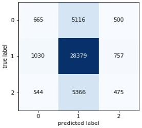
(b) CTL 2Layers

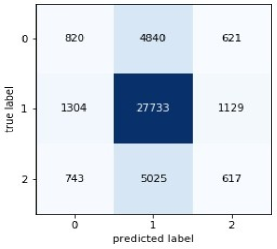
(c) CTL 3Layers

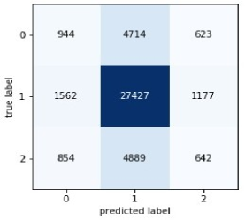
(d) CTL 4Layers

Figure 4: Confusion matrices corresponding to the different number of CTL layers of the architecture: a) 1 layer of CTL (shallow version), b) 2 layers of CTL (deep version), c) 3 layers of CTL (deep version) and d) 4 layers of CTL (deep version) where 0 - BUY, 1 - HOLD, 2 - SELL signals.

To better analyze the framework performance, we calculate the weighted F1 score, precision and recall metric values for all the stocks under consideration. We calculate the weighted values to incorporate the class imbalance for every stock. The detailed and summary results are given in Table LABEL:a_weighted_detailed in A and Table 6. Again, the results comprise two sets of values marked in bold or red with the same err_dif of 0.02. There are 6, 9, and 5 stocks with respect to the metrics F1 score, precision and recall for which the model performs greater than or equal to the performance given by the state-of-the-arts. Also, there are 6, 3 and 6 stocks for the metrics F1 score, precision and recall respectively for which the model gives the next best performance under 0.02 err_dif. Although the BUY and SELL classes performance with the 4 CTL Layers deep architecture is better than the benchmarks compared against, but the overall performance from the average weighted metric is suggestive of the good performance with the 3 layers deep architecture classification wisely. This is also suggested from the financial results explained later.

Again analyzing explicitly for CNN, we have 4, 2 and 7 stocks with greater than or equal performance; and 3, 2 and 3 stocks under similar/next best performance for the metrics F1 score, precision and recall respectively. As can be referenced from the statistics presented here, our model is giving better results with greater than or equal and the next best/similar performances except for the number of stocks for recall metric are slightly more with CNN under greater than or equal to performance. However, the next best performance statistic for the recall metric is much better than CNN. Overall performance on an average is good with our proposed model as compared to the benchmarks and CNN which can be also referred from Table 6. For a deeper understanding of the aforementioned statistics, please refer to Table LABEL:comparison in  C.

Table 6: Summary of Weighted Classification Results for Stock Trading

Method	Avg. F1 Score	Avg. Precision	Avg. Recall
SDCF 1L	0.6169	0.6216	0.6941
SDCF 2L	0.6229	0.6207	0.6867
SDCF 3L	0.6250	0.6146	0.6784
SDCF 4L	0.5345	0.5464	0.5890
CNN	0.6182	0.5907	0.6898
FCN	0.6090	0.6079	0.6725
CNN-TA	0.6148	0.6161	0.6575
MFNN	0.4162	0.5509	0.4676

5.2 Financial Analysis

It is very important to analyse the performance from a financial perspective to understand the quality of predictions made by our model. For this, as explained earlier, we have calculated the AR values with the predictions generated by each of the techniques for every stock over 11 years. We also calculate the AR values with the True labels for every stock over the same period. Finally, we calculate the absolute difference/error between the AR values from Predictions and the AR values from True labels. We average the absolute difference values for all stocks yielding the so-called Mean Absolute Error. The detailed results are given in Table LABEL:b_detailed. With our proposed model 5 stocks have the best performance whereas with CNN-TA there is 1 stock and 2 stocks under MFNN and FCN. On the whole, the performance is good with our proposed model as also evident from the summary results in Table 7 where we have a mean of the absolute difference/error(MAE) between the True AR and Predicted AR. Also, there are 3 stocks for which the proposed model gives an equal performance as the other benchmark techniques. Here, this set of results is illustrating that, despite the higher capability of identifying the BUY and SELL points with 4 layers deep CTL, the AR values are better predicted with the 3 layers deep CTL framework.

With respect to CNN, there are only 2 stocks for which CNN performs better than any benchmarks and our proposed models, and 3 stocks for which it gives an equal performance. Thus, from the combined (greater than or equal to and next best / similar), average and the financial results, the CNN results are less performant than our model. This also indicates that the quality of predictions made with our model is better than CNN as the identified class labels give AR values quite close to the True AR values. This remains true for all the benchmarks. The statistics presented here can be deduced from Table LABEL:comparison in  C for complete understanding.

Table 7: Summary of Financial Results for Stock Trading

Method	MAE AR
SDCF 1L	22.5613
SDCF 2L	20.7227
SDCF 3L	20.5067
SDCF 4L	22.8287
CNN	21.1140
FCN	23.7720
CNN-TA	22.1380
MFNN	22.3040

To further understand the better supervised learning for both regular CNN and our SDCF framework, we visualize channel-wise $X_{c}$ features for both the frameworks which are obtained after the last maxpool layer for the 3 convolutional layers deep framework. The following Figure 5 shows the visualizations of the features for one sample of the stock ‘BSELINFRA.BO’.

Features generated by the proposed SDCF network.
Features generated by a standard CNN with a similar architecture.

(a) Channel $X_{1}$ Close Price

(b) Channel $X_{2}$ Open Price

(c) Channel $X_{3}$ High Price

(d) Channel $X_{4}$ Low Price

(e) Channel $X_{5}$ NAV

Figure 5: Visualization of channel-wise features $X_{c}$ for SDCF versus a standard CNN, for one sample of stock BSELINFRA.BO (with 16x1 as the shape of the features obtained and resized to 8x2 for better visualization)

As can be seen from Figure 5, heatmap for each channel corresponding to the prices(Close, Open, High and Low) show no variation in the case of CNN as compared to the SDCF architecture. While it shows some variations for the features learnt corresponding to NAV, however, the features are still better learnt with SDCF. Also, darker the color in the heatmap, more it is indicative of the larger negative exponent values. In the case of CNN, hence, the values are very very small that are almost diminishing to zero. This also corroborates the fact that the filters learnt with our model are distinct due to the “log-det” term added which further gives different features with very less redundancy. Thus, the visualizations of these channel-wise features are also supportive of better supervised training with our framework than CNN.

In order to test our architecture’s capability further, we have performed experiments for two additional window sizes, namely 5 and 20. In order to avoid extensive space utilization, we present here only the comparative summary results - Weighted F1 Score(Classification Metric) and MAE AR(Financial metric) in Table 8 for window sizes 5 and 20 along with the summarized results for window size 10. Our method yields the best results on an aggregate. Even though CNN-TA yields better AR for a solo case (window size 20), it does not reach better results in terms of weighted F1 for the same scenario. Furthermore, CNN-TA cannot be run for all small window sizes (such as 5), hence cannot be deemed as an all-purpose go-to method. Small window sizes are crucial for highly non-stationary stocks and the inability of a method to handle such stocks is a major shortcoming. Overall, our model performs better than benchmarks and CNN both classification-wise and financially, specifically, it gives the best performance with 3 CTL layers deep SDCF framework of all the 4 SDCF architectures. We also display the empirical convergence plots for a few stocks, namely INDRAMEDCO.BO and NATIONALUM.BO in Figure 6 for both shallow and deeper versions. We can see that the training loss decreases to a point of stability for each example considered.

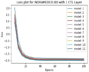
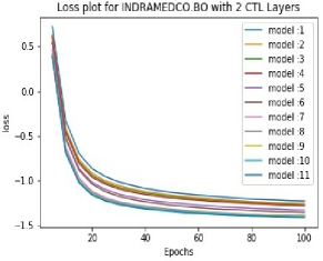
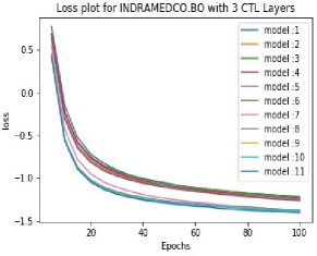
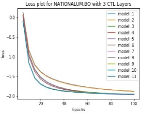
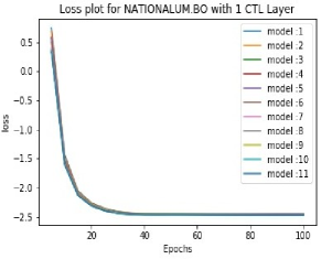
(a) CTL 1 layer

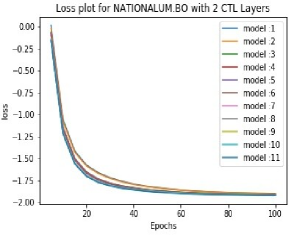
(b) CTL 2 layers

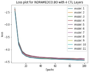
(c) CTL 3 layers

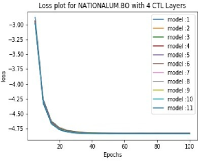
(d) CTL 4 layers

Figure 6: Evolution of the loss during training for few stock examples, of our proposed model with (a) CTL 1 layer, (b) CTL 2 layers, (c) CTL 3 layers and (d) CTL 4 layers.

Table 8: Comparative Summary Results for Stock Trading for window sizes 5,10,20

Method	Window Size 5		Window Size 10		Window Size 10
	F1	MAE AR	F1	MAE AR	F1	MAE AR
SDCF 1L	0.6141	22.4947	0.6169	22.5613	0.6194	22.4453
SDCF 2L	0.6148	24.3820	0.6229	20.7227	0.6242	25.0200
SDCF 3L	0.6207	20.9193	0.6250	20.5067	0.6262	25.7667
SDCF 4L	0.6157	21.5427	0.5345	22.8287	0.6254	26.1007
CNN	0.6095	22.0113	0.6182	21.1140	0.6217	22.9560
FCN	0.6131	23.3107	0.6090	23.7720	0.6120	24.2233
CNN-TA*	-	-	0.6148	22.1380	0.6246	20.3820
MFNN	0.4105	23.4820	0.4162	22.3040	0.4869	23.2620

• *CNN-TA cannot be run for window size 5 due to its inherent structure

6 Conclusion

In this work, we propose SDCF, a deep fusion end-to-end framework for the processing of stock trading data. Unlike other deep learning models, our framework is a fusion supervised framework. It relies on a novel deep version of our recently proposed CTL model. We have applied the proposed model for stock trading leading to very good performance. In particular, the classification results are better with the proposed SDCF model, than with the 1-D CNN approach. Also, the features $X_{c}$ visualized for each channel and each method indicate the better feature learning with SDCF. The results show that the proposed solution is superior to CNN and other state-of-the arts techniques in this problem.

We believe that the framework is generic enough to handle other multi-channel fusion problems as well. In the future, we plan to extend the application to other fusion 1-D as well as 2-D multi-channel problems to test its generality. For example, we plan to implement it in the biomedical domain to analyse PPG and ECG signals for the blood pressure estimation pertaining to the 1-D multi-channel problem. In case of 2-D problems, we would like to do multi-spectral image classification using this technique. Currently, the shortcoming with our model is that it takes slightly more time than CNN, for its training. Thus, we will investigate on the reduction of the time complexity of our framework in order to make it more efficient from this viewpoint.

The current purpose of our paper is to introduce our new algorithm and to show by means of several experiments that it is an effective tool for predicting stocks. However, stock price prediction may be seen as a too rudimentary problem in financial analytics. As a next step, we would like to investigate the use of our algorithm to study if it can emulate (human) expert-like suggestions. For example, fund managers suggest ‘buy stock XYZ at a price ABC’ or ‘sell stock ZYX at price CBA’. We would like to see if our algorithm can make such predictions given a time horizon. If possible, we would like to extend the algorithm to emulate more abstract financial operations such as ‘hedging (longs and shorts)’.

7 Acknowledgement

This work was supported by the CNRS-CEFIPRA project under grant NextGenBP PRC2017.

Appendix A Class-Wise Classification Results for Stock Trading

This section displays all the tables with the Classification Metrics results, both class-wise and weighted, for stock trading.

Table 9: Classification Results for BUY Class for Stock Trading

SYMBOL	Method	BUY F1 Score	BUY Precision	BUY Recall
ALKYLAMINE.BO	SDCF 1L	0.1022	0.2450	0.0646
	SDCF 2L	0.1708	0.2222	0.1387
	SDCF 3L	0.1670	0.2056	0.1407
	SDCF 4L	0.1880	0.2500	0.1507
	CNN	0.1678	0.2458	0.1274
	FCN	0.1131	0.2484	0.0732
	CNN-TA	0.0924	0.2308	0.0578
	MFNN	0.1205	0.1974	0.0867
AUROPHARMA.NS	SDCF 1L	0.0000	0.0000	0.0000
	SDCF 2L	0.0000	0.0000	0.0000
	SDCF 3L	0.0048	0.3333	0.0024
	SDCF 4L	0.0299	0.5000	0.0154
	CNN	0.0000	0.0000	0.0000
	FCN	0.0000	0.0000	0.0000
	CNN-TA	0.0814	0.2121	0.0504
	MFNN	0.0046	0.0625	0.0024
BPCL.NS	SDCF 1L	0.0238	0.3125	0.0124
	SDCF 2L	0.0318	0.3333	0.0167
	SDCF 3L	0.0054	0.1250	0.0028
	SDCF 4L	0.0988	0.4000	0.0563
	CNN	0.0000	0.0000	0.0000
	FCN	0.2275	0.2628	0.2006
	CNN-TA	0.0000	0.0000	0.0000
	MFNN	0.0107	0.1250	0.0056
BSELINFRA.BO	SDCF 1L	0.0000	0.0000	0.0000
	SDCF 2L	0.0000	0.0000	0.0000
	SDCF 3L	0.0000	0.0000	0.0000
	SDCF 4L	0.0000	0.0000	0.0000
	CNN	0.0000	0.0000	0.0000
	FCN	0.0000	0.0000	0.0000
	CNN-TA	0.0000	0.0000	0.0000
	MFNN	0.0000	0.0000	0.0000
CAIRN.NS	SDCF 1L	0.0744	0.3523	0.0416
	SDCF 2L	0.2201	0.3646	0.1577
	SDCF 3L	0.2348	0.3371	0.1802
	SDCF 4L	0.3179	0.4068	0.2609
	CNN	0.1212	0.3699	0.0725
	FCN	0.0313	0.2895	0.0165
	CNN-TA	0.2405	0.3023	0.1997
	MFNN	0.0453	0.4000	0.0240
DEEPAKSP.BO	SDCF 1L	0.1106	0.2293	0.0729
	SDCF 2L	0.1280	0.2213	0.0900
	SDCF 3L	0.1427	0.2305	0.1033
	SDCF 4L	0.1818	0.2895	0.1325
	CNN	0.1300	0.2243	0.0915
	FCN	0.1437	0.2450	0.1017
	CNN-TA	0.2590	0.2319	0.2933
	MFNN	0.0457	0.2679	0.0250
DRREDDY.NS	SDCF 1L	0.0134	0.1053	0.0072
	SDCF 2L	0.0227	0.3750	0.0117
	SDCF 3L	0.0148	0.1429	0.0078
	SDCF 4L	0.0755	0.5000	0.0408
	CNN	0.0000	0.0000	0.0000
	FCN	0.0148	0.1429	0.0078
	CNN-TA	0.1192	0.1769	0.0898
	MFNN	0.1790	0.0985	0.9805
HCC.NS	SDCF 1L	0.0238	0.0556	0.0152
	SDCF 2L	0.0274	0.1000	0.0159
	SDCF 3L	0.0290	0.1667	0.0159
	SDCF 4L	0.0800	1.0000	0.0417
	CNN	0.0000	0.0000	0.0000
	FCN	0.0471	0.0909	0.0317
	CNN-TA	0.0370	0.0197	0.3016
	MFNN	0.0392	0.0203	0.6032
HINDPETRO.NS	SDCF 1L	0.0000	0.0000	0.0000
	SDCF 2L	0.0000	0.0000	0.0000
	SDCF 3L	0.0000	0.0000	0.0000
	SDCF 4L	0.0000	0.0000	0.0000
	CNN	0.0000	0.0000	0.0000
	FCN	0.0377	0.0500	0.0303
	CNN-TA	0.0000	0.0000	0.0000
	MFNN	0.0543	0.0319	0.1818
INDRAMEDCO.BO	SDCF 1L	0.0744	0.3523	0.0416
	SDCF 2L	0.2201	0.3646	0.1577
	SDCF 3L	0.2474	0.3377	0.1952
	SDCF 4L	0.3358	0.5111	0.2500
	CNN	0.1212	0.3699	0.0725
	FCN	0.0313	0.2895	0.0165
	CNN-TA	0.2972	0.3446	0.2613
	MFNN	0.0143	0.4167	0.0073
IOC.BO	SDCF 1L	0.0976	0.5000	0.0541
	SDCF 2L	0.1026	0.5000	0.0571
	SDCF 3L	0.1026	0.5000	0.0571
	SDCF 4L	0.0000	0.0000	0.0000
	CNN	0.0000	0.0000	0.0000
	FCN	0.0533	0.0500	0.0571
	CNN-TA	0.0000	0.0000	0.0000
	MFNN	0.0267	0.0250	0.0286
KENNAMET.BO	SDCF 1L	0.3173	0.3137	0.3210
	SDCF 2L	0.2771	0.3303	0.2387
	SDCF 3L	0.2857	0.3160	0.2607
	SDCF 4L	0.3662	0.3611	0.3714
	CNN	0.3236	0.3131	0.3349
	FCN	0.2792	0.3078	0.2555
	CNN-TA	0.3558	0.3224	0.3969
	MFNN	0.0269	0.3667	0.0140
NATIONALUM.BO	SDCF 1L	0.0000	0.0000	0.0000
	SDCF 2L	0.0000	0.0000	0.0000
	SDCF 3L	0.0000	0.0000	0.0000
	SDCF 4L	0.0000	0.0000	0.0000
	CNN	0.0000	0.0000	0.0000
	FCN	0.0000	0.0000	0.0000
	CNN-TA	0.0000	0.0000	0.0000
	MFNN	0.0000	0.0000	0.0000
NATIONALUM.NS	SDCF 1L	0.0025	0.5000	0.0013
	SDCF 2L	0.0026	0.5000	0.0013
	SDCF 3L	0.1775	0.3516	0.1187
	SDCF 4L	0.3576	0.3253	0.3971
	CNN	0.0000	0.0000	0.0000
	FCN	0.0000	0.0000	0.0000
	CNN-TA	0.2471	0.3286	0.1980
	MFNN	0.4342	0.2987	0.7949
NITINALOY.BO	SDCF 1L	0.1272	0.3067	0.0803
	SDCF 2L	0.1708	0.2222	0.1387
	SDCF 3L	0.2242	0.2609	0.1965
	SDCF 4L	0.3172	0.3194	0.3151
	CNN	0.1678	0.2458	0.1274
	FCN	0.1587	0.1928	0.1349
	CNN-TA	0.0779	0.2474	0.0462
	MFNN	0.3208	0.1978	0.8478

Table 10: Classification Results for HOLD Class for Stock Trading

SYMBOL	Method	HOLD F1 Score	HOLD Precision	HOLD Recall
ALKYLAMINE.BO	SDCF 1L	0.7216	0.6062	0.8912
	SDCF 2L	0.6932	0.6137	0.7963
	SDCF 3L	0.6762	0.6113	0.7565
	SDCF 4L	0.5761	0.5072	0.6667
	CNN	0.7214	0.6196	0.8632
	FCN	0.7318	0.6060	0.9236
	CNN-TA	0.7298	0.5951	0.9432
	MFNN	0.0906	0.6048	0.0490
AUROPHARMA.NS	SDCF 1L	0.7887	0.6523	0.9973
	SDCF 2L	0.7849	0.6474	0.9964
	SDCF 3L	0.7850	0.6473	0.9970
	SDCF 4L	0.7024	0.5458	0.9850
	CNN	0.7878	0.6499	1.0000
	FCN	0.7815	0.6480	0.9845
	CNN-TA	0.7722	0.6524	0.9457
	MFNN	0.0661	0.5463	0.0352
BPCL.NS	SDCF 1L	0.8136	0.6891	0.9930
	SDCF 2L	0.8158	0.6927	0.9922
	SDCF 3L	0.8153	0.6912	0.9939
	SDCF 4L	0.5982	0.4322	0.9714
	CNN	0.8152	0.6880	1.0000
	FCN	0.8085	0.7169	0.9271
	CNN-TA	0.8138	0.6914	0.9889
	MFNN	0.8068	0.6904	0.9705
BSELINFRA.BO	SDCF 1L	0.9860	0.9723	1.0000
	SDCF 2L	0.9881	0.9765	1.0000
	SDCF 3L	0.9881	0.9765	1.0000
	SDCF 4L	0.9918	0.9837	1.0000
	CNN	0.9860	0.9723	1.0000
	FCN	0.9782	0.9761	0.9803
	CNN-TA	0.9840	0.9763	0.9917
	MFNN	0.4514	0.9751	0.2937
CAIRN.NS	SDCF 1L	0.6850	0.5274	0.9768
	SDCF 2L	0.6738	0.5364	0.9060
	SDCF 3L	0.6698	0.5390	0.8845
	SDCF 4L	0.5019	0.3860	0.7174
	CNN	0.6812	0.5299	0.9535
	FCN	0.6804	0.5217	0.9778
	CNN-TA	0.6613	0.5567	0.8142
	MFNN	0.6806	0.5249	0.9674
DEEPAKSP.BO	SDCF 1L	0.6771	0.5564	0.8648
	SDCF 2L	0.6426	0.5380	0.7977
	SDCF 3L	0.6261	0.5395	0.7460
	SDCF 4L	0.4925	0.3837	0.6875
	CNN	0.6517	0.5497	0.8000
	FCN	0.6463	0.5488	0.7860
	CNN-TA	0.5636	0.5404	0.5888
	MFNN	0.6872	0.5338	0.9643
DRREDDY.NS	SDCF 1L	0.8810	0.7920	0.9926
	SDCF 2L	0.8799	0.7879	0.9961
	SDCF 3L	0.8761	0.7893	0.9843
	SDCF 4L	0.7558	0.6176	0.9735
	CNN	0.8833	0.7910	1.0000
	FCN	0.8771	0.7872	0.9902
	CNN-TA	0.8548	0.7970	0.9217
	MFNN	0.0000	0.0000	0.0000
HCC.NS	SDCF 1L	0.9660	0.9417	0.9915
	SDCF 2L	0.9667	0.9411	0.9939
	SDCF 3L	0.9668	0.9404	0.9947
	SDCF 4L	0.8989	0.8163	1.0000
	CNN	0.9697	0.9412	1.0000
	FCN	0.9254	0.9535	0.8989
	CNN-TA	0.7497	0.9368	0.6249
	MFNN	0.4091	0.9263	0.2625
HINDPETRO.NS	SDCF 1L	0.9688	0.9401	0.9993
	SDCF 2L	0.9690	0.9407	0.9992
	SDCF 3L	0.9690	0.9407	0.9992
	SDCF 4L	0.9135	0.8408	1.0000
	CNN	0.9691	0.9401	1.0000
	FCN	0.8844	0.9545	0.8240
	CNN-TA	0.9686	0.9406	0.9984
	MFNN	0.8979	0.9428	0.8571
INDRAMEDCO.BO	SDCF 1L	0.6850	0.5274	0.9768
	SDCF 2L	0.6738	0.5364	0.9060
	SDCF 3L	0.6678	0.5403	0.8742
	SDCF 4L	0.5196	0.3862	0.7935
	CNN	0.6812	0.5299	0.9535
	FCN	0.6804	0.5217	0.9778
	CNN-TA	0.6569	0.5665	0.7816
	MFNN	0.6755	0.5202	0.9630
IOC.BO	SDCF 1L	0.9817	0.9647	0.9993
	SDCF 2L	0.9810	0.9634	0.9992
	SDCF 3L	0.9810	0.9634	0.9992
	SDCF 4L	0.9325	0.8735	1.0000
	CNN	0.9817	0.9640	1.0000
	FCN	0.9737	0.9628	0.9848
	CNN-TA	0.9808	0.9624	1.0000
	MFNN	0.9737	0.9628	0.9848
KENNAMET.BO	SDCF 1L	0.5067	0.4475	0.5840
	SDCF 2L	0.5201	0.4664	0.5878
	SDCF 3L	0.4585	0.4407	0.4779
	SDCF 4L	0.2419	0.2459	0.2381
	CNN	0.4243	0.4236	0.4250
	FCN	0.5202	0.4568	0.6040
	CNN-TA	0.5381	0.4619	0.6445
	MFNN	0.6001	0.4297	0.9947
NATIONALUM.BO	SDCF 1L	0.9983	0.9966	1.0000
	SDCF 2L	0.9984	0.9968	1.0000
	SDCF 3L	0.9984	0.9968	1.0000
	SDCF 4L	0.9959	0.9918	1.0000
	CNN	0.9983	0.9966	1.0000
	FCN	0.9888	0.9968	0.9810
	CNN-TA	0.9983	0.9966	1.0000
	MFNN	0.9775	0.9965	0.9592
NATIONALUM.NS	SDCF 1L	0.5892	0.4188	0.9937
	SDCF 2L	0.5869	0.4190	0.9792
	SDCF 3L	0.5525	0.4242	0.7919
	SDCF 4L	0.4000	0.4429	0.3647
	CNN	0.5905	0.4189	1.0000
	FCN	0.5857	0.4171	0.9830
	CNN-TA	0.5258	0.4463	0.6397
	MFNN	0.2237	0.4171	0.1528
NITINALOY.BO	SDCF 1L	0.7252	0.6036	0.9082
	SDCF 2L	0.6932	0.6137	0.7963
	SDCF 3L	0.6891	0.6282	0.7631
	SDCF 4L	0.5044	0.4711	0.5429
	CNN	0.7214	0.6196	0.8632
	FCN	0.6746	0.6105	0.7539
	CNN-TA	0.7305	0.5927	0.9517
	MFNN	0.2017	0.5663	0.1227

Table 11: Classification Results for SELL Class for Stock Trading

SYMBOL	Method	SELL F1 Score	SELL Precision	SELL Recall
ALKYLAMINE.BO	SDCF 1L	0.1207	0.2279	0.0821
	SDCF 2L	0.1820	0.2681	0.1378
	SDCF 3L	0.1945	0.2522	0.1583
	SDCF 4L	0.3594	0.3710	0.3485
	CNN	0.1278	0.2537	0.0854
	FCN	0.0879	0.2800	0.0521
	CNN-TA	0.0282	0.2667	0.0149
	MFNN	0.3347	0.2075	0.8641
AUROPHARMA.NS	SDCF 1L	0.0178	0.3333	0.0092
	SDCF 2L	0.0193	0.3571	0.0099
	SDCF 3L	0.0194	0.4167	0.0099
	SDCF 4L	0.0385	0.2500	0.0208
	CNN	0.0000	0.0000	0.0000
	FCN	0.0510	0.3111	0.0278
	CNN-TA	0.0524	0.2206	0.0298
	MFNN	0.3210	0.1932	0.9484
BPCL.NS	SDCF 1L	0.0039	0.1111	0.0020
	SDCF 2L	0.0000	0.0000	0.0000
	SDCF 3L	0.0000	0.0000	0.0000
	SDCF 4L	0.0000	0.0000	0.0000
	CNN	0.0000	0.0000	0.0000
	FCN	0.0000	0.0000	0.0000
	CNN-TA	0.0213	0.1786	0.0113
	MFNN	0.0321	0.1429	0.0181
BSELINFRA.BO	SDCF 1L	0.0000	0.0000	0.0000
	SDCF 2L	0.0000	0.0000	0.0000
	SDCF 3L	0.0000	0.0000	0.0000
	SDCF 4L	0.0000	0.0000	0.0000
	CNN	0.0000	0.0000	0.0000
	FCN	0.0000	0.0000	0.0000
	CNN-TA	0.0000	0.0000	0.0000
	MFNN	0.0319	0.0164	0.6383
CAIRN.NS	SDCF 1L	0.0183	0.4286	0.0094
	SDCF 2L	0.0230	0.2500	0.0120
	SDCF 3L	0.0231	0.2800	0.0120
	SDCF 4L	0.1282	0.3125	0.0806
	CNN	0.0207	0.2000	0.0109
	FCN	0.0197	0.2143	0.0103
	CNN-TA	0.1337	0.2800	0.0879
	MFNN	0.0431	0.2059	0.0241
DEEPAKSP.BO	SDCF 1L	0.1140	0.2252	0.0763
	SDCF 2L	0.1914	0.2890	0.1431
	SDCF 3L	0.2174	0.2688	0.1826
	SDCF 4L	0.2772	0.4000	0.2121
	CNN	0.1436	0.2188	0.1069
	FCN	0.2302	0.3068	0.1842
	CNN-TA	0.1799	0.2577	0.1382
	MFNN	0.0245	0.1818	0.0132
DRREDDY.NS	SDCF 1L	0.0060	0.1667	0.0031
	SDCF 2L	0.0066	0.2000	0.0034
	SDCF 3L	0.0363	0.1765	0.0202
	SDCF 4L	0.0417	0.3333	0.0222
	CNN	0.0000	0.0000	0.0000
	FCN	0.0129	0.1667	0.0067
	CNN-TA	0.0700	0.1359	0.0471
	MFNN	0.0116	0.0417	0.0067
HCC.NS	SDCF 1L	0.0000	0.0000	0.0000
	SDCF 2L	0.0392	0.2222	0.0215
	SDCF 3L	0.0000	0.0000	0.0000
	SDCF 4L	0.0000	0.0000	0.0000
	CNN	0.0000	0.0000	0.0000
	FCN	0.1090	0.0730	0.2151
	CNN-TA	0.0204	0.2000	0.0108
	MFNN	0.0000	0.0000	0.0000
HINDPETRO.NS	SDCF 1L	0.0000	0.0000	0.0000
	SDCF 2L	0.0000	0.0000	0.0000
	SDCF 3L	0.0000	0.0000	0.0000
	SDCF 4L	0.0000	0.0000	0.0000
	CNN	0.0000	0.0000	0.0000
	FCN	0.1007	0.0603	0.3068
	CNN-TA	0.0000	0.0000	0.0000
	MFNN	0.0000	0.0000	0.0000
INDRAMEDCO.BO	SDCF 1L	0.0183	0.4286	0.0094
	SDCF 2L	0.0230	0.2500	0.0120
	SDCF 3L	0.0164	0.1852	0.0086
	SDCF 4L	0.1081	0.3333	0.0645
	CNN	0.0207	0.2000	0.0109
	FCN	0.0197	0.2143	0.0103
	CNN-TA	0.1506	0.2664	0.1050
	MFNN	0.0587	0.2174	0.0339
IOC.BO	SDCF 1L	0.0000	0.0000	0.0000
	SDCF 2L	0.0000	0.0000	0.0000
	SDCF 3L	0.0000	0.0000	0.0000
	SDCF 4L	0.0000	0.0000	0.0000
	CNN	0.0000	0.0000	0.0000
	FCN	0.0000	0.0000	0.0000
	CNN-TA	0.0000	0.0000	0.0000
	MFNN	0.0000	0.0000	0.0000
KENNAMET.BO	SDCF 1L	0.2050	0.3039	0.1546
	SDCF 2L	0.2697	0.2855	0.2556
	SDCF 3L	0.2960	0.2880	0.3045
	SDCF 4L	0.4387	0.4416	0.4359
	CNN	0.2805	0.2927	0.2693
	FCN	0.2739	0.3374	0.2304
	CNN-TA	0.0883	0.3636	0.0503
	MFNN	0.0000	0.0000	0.0000
NATIONALUM.BO	SDCF 1L	0.0000	0.0000	0.0000
	SDCF 2L	0.0000	0.0000	0.0000
	SDCF 3L	0.0000	0.0000	0.0000
	SDCF 4L	0.0000	0.0000	0.0000
	CNN	0.0000	0.0000	0.0000
	FCN	0.0000	0.0000	0.0000
	CNN-TA	0.0000	0.0000	0.0000
	MFNN	0.0000	0.0000	0.0000
NATIONALUM.NS	SDCF 1L	0.0053	0.1429	0.0027
	SDCF 2L	0.0383	0.2381	0.0208
	SDCF 3L	0.1540	0.2582	0.1097
	SDCF 4L	0.4333	0.4333	0.4333
	CNN	0.0000	0.0000	0.0000
	FCN	0.0340	0.2955	0.0181
	CNN-TA	0.2527	0.2887	0.2247
	MFNN	0.0821	0.2500	0.0491
NITINALOY.BO	SDCF 1L	0.1247	0.2994	0.0787
	SDCF 2L	0.1820	0.2681	0.1378
	SDCF 3L	0.1810	0.2351	0.1471
	SDCF 4L	0.2906	0.3333	0.2576
	CNN	0.1278	0.2537	0.0854
	FCN	0.1747	0.2282	0.1415
	CNN-TA	0.0211	0.1935	0.0112
	MFNN	0.0105	0.0938	0.0056

Table 12: Weighted Classification Results for Stock Trading

SYMBOL	Method	F1 Score	Precision	Recall
ALKYLAMINE.BO	SDCF 1L	0.4738	0.4559	0.5590
	SDCF 2L	0.4824	0.4635	0.5278
	SDCF 3L	0.4741	0.4554	0.5089
	SDCF 4L	0.4014	0.3934	0.4262
	CNN	0.4882	0.4694	0.5556
	FCN	0.4741	0.4666	0.5723
	CNN-TA	0.4564	0.4539	0.5730
	MFNN	0.1472	0.4407	0.2257
AUROPHARMA.NS	SDCF 1L	0.5160	0.4869	0.6499
	SDCF 2L	0.5104	0.4872	0.6451
	SDCF 3L	0.5112	0.5522	0.6459
	SDCF 4L	0.3952	0.4760	0.5407
	CNN	0.5121	0.4224	0.6499
	FCN	0.5144	0.4786	0.6409
	CNN-TA	0.5217	0.4980	0.6243
	MFNN	0.1057	0.4001	0.2071
BPCL.NS	SDCF 1L	0.5638	0.5369	0.6852
	SDCF 2L	0.5687	0.5252	0.6886
	SDCF 3L	0.5647	0.4953	0.6878
	SDCF 4L	0.2839	0.2999	0.4309
	CNN	0.5608	0.4733	0.6880
	FCN	0.5907	0.5322	0.6690
	CNN-TA	0.5665	0.5086	0.6859
	MFNN	0.5650	0.5191	0.6751
BSELINFRA.BO	SDCF 1L	0.9587	0.9454	0.9723
	SDCF 2L	0.9649	0.9536	0.9765
	SDCF 3L	0.9649	0.9536	0.9765
	SDCF 4L	0.9757	0.9677	0.9837
	CNN	0.9587	0.9454	0.9723
	FCN	0.9552	0.9531	0.9573
	CNN-TA	0.9609	0.9534	0.9684
	MFNN	0.4414	0.9525	0.2983
CAIRN.NS	SDCF 1L	0.3801	0.4604	0.5216
	SDCF 2L	0.4120	0.4283	0.5142
	SDCF 3L	0.4137	0.4293	0.5089
	SDCF 4L	0.3389	0.3752	0.3862
	CNN	0.3907	0.4156	0.5178
	FCN	0.3662	0.3934	0.5150
	CNN-TA	0.4354	0.4296	0.4942
	MFNN	0.3752	0.4215	0.5146
DEEPAKSP.BO	SDCF 1L	0.4217	0.4075	0.5075
	SDCF 2L	0.4168	0.4058	0.4791
	SDCF 3L	0.4176	0.4039	0.4640
	SDCF 4L	0.3293	0.3562	0.3714
	CNN	0.4189	0.4013	0.4831
	FCN	0.4315	0.4212	0.4853
	CNN-TA	0.4024	0.4021	0.4140
	MFNN	0.3821	0.3891	0.5221
DRREDDY.NS	SDCF 1L	0.6988	0.6554	0.7862
	SDCF 2L	0.6955	0.6800	0.7855
	SDCF 3L	0.6952	0.6555	0.7778
	SDCF 4L	0.4886	0.5419	0.6122
	CNN	0.6987	0.6257	0.7910
	FCN	0.6933	0.6528	0.7809
	CNN-TA	0.6925	0.6602	0.7397
	MFNN	0.0190	0.0145	0.0974
HCC.NS	SDCF 1L	0.9097	0.8876	0.9336
	SDCF 2L	0.9108	0.8949	0.9353
	SDCF 3L	0.9094	0.8880	0.9353
	SDCF 4L	0.7386	0.7612	0.8171
	CNN	0.9127	0.8859	0.9412
	FCN	0.8749	0.9011	0.8533
	CNN-TA	0.7063	0.8882	0.5951
	MFNN	0.3855	0.8712	0.2614
HINDPETRO.NS	SDCF 1L	0.9108	0.8838	0.9394
	SDCF 2L	0.9116	0.8849	0.9399
	SDCF 3L	0.9116	0.8849	0.9399
	SDCF 4L	0.7681	0.7070	0.8408
	CNN	0.9111	0.8839	0.9401
	FCN	0.8364	0.9012	0.7863
	CNN-TA	0.9112	0.8848	0.9392
	MFNN	0.8461	0.8877	0.8109
INDRAMEDCO.BO	SDCF 1L	0.3801	0.4604	0.5216
	SDCF 2L	0.4120	0.4283	0.5142
	SDCF 3L	0.4144	0.4089	0.5065
	SDCF 4L	0.3471	0.4196	0.4065
	CNN	0.4316	0.4621	0.5223
	FCN	0.3662	0.3934	0.5150
	CNN-TA	0.4517	0.4425	0.4969
	MFNN	0.3681	0.4259	0.5102
IOC.BO	SDCF 1L	0.9476	0.9363	0.9640
	SDCF 2L	0.9457	0.9341	0.9626
	SDCF 3L	0.9457	0.9341	0.9626
	SDCF 4L	0.8145	0.7629	0.8735
	CNN	0.9456	0.9293	0.9634
	FCN	0.9381	0.9276	0.9488
	CNN-TA	0.9443	0.9267	0.9626
	MFNN	0.9377	0.9272	0.9484
KENNAMET.BO	SDCF 1L	0.3665	0.3677	0.3864
	SDCF 2L	0.3790	0.3762	0.3926
	SDCF 3L	0.3625	0.3616	0.3657
	SDCF 4L	0.3574	0.3571	0.3577
	CNN	0.3705	0.3709	0.3715
	FCN	0.3808	0.3797	0.3976
	CNN-TA	0.3601	0.3934	0.4072
	MFNN	0.2646	0.2926	0.4295
NATIONALUM.BO	SDCF 1L	0.9949	0.9932	0.9966
	SDCF 2L	0.9953	0.9937	0.9968
	SDCF 3L	0.9953	0.9937	0.9968
	SDCF 4L	0.9877	0.9836	0.9918
	CNN	0.9949	0.9932	0.9966
	FCN	0.9857	0.9936	0.9779
	CNN-TA	0.9949	0.9932	0.9966
	MFNN	0.9742	0.9931	0.9560
NATIONALUM.NS	SDCF 1L	0.2491	0.3655	0.4174
	SDCF 2L	0.2564	0.3919	0.4146
	SDCF 3L	0.3272	0.3553	0.3968
	SDCF 4L	0.4005	0.4064	0.3992
	CNN	0.2473	0.1755	0.4189
	FCN	0.2539	0.2578	0.4150
	CNN-TA	0.3653	0.3665	0.3903
	MFNN	0.2460	0.3344	0.3141
NITINALOY.BO	SDCF 1L	0.4817	0.4814	0.5715
	SDCF 2L	0.4824	0.4635	0.5278
	SDCF 3L	0.4675	0.4474	0.5027
	SDCF 4L	0.3906	0.3885	0.3975
	CNN	0.4956	0.4786	0.5455
	FCN	0.4741	0.4666	0.5723
	CNN-TA	0.4524	0.4406	0.5750
	MFNN	0.1859	0.3943	0.2438

Appendix B Financial Results for Stock Trading

This section mentions the table with financial results for stock trading for all the stocks.

Table 13: Financial Results for Stock Trading

SYMBOL	Method	True AR	Predicted AR	Absolute Difference AR
ALKYLAMINE.BO	SDCF 1L	86.3000	5.7500	80.5500
	SDCF 2L		12.3000	74.0000
	SDCF 3L		25.9600	60.3400
	SDCF 4L		10.3700	75.9300
	CNN		8.2300	78.0700
	FCN		1.6500	84.6500
	CNN-TA		14.6200	71.6800
	MFNN		6.4200	79.8800
AUROPHARMA.NS	SDCF 1L	-0.8300	9.9400	10.7700
	SDCF 2L		9.9200	10.7500
	SDCF 3L		10.5700	11.4000
	SDCF 4L		10.3300	11.1600
	CNN		0.0000	0.8300
	FCN		9.2100	10.0400
	CNN-TA		19.7400	20.5700
	MFNN		0.6200	1.4500
BPCL.NS	SDCF 1L	14.1200	0.7800	13.3400
	SDCF 2L		0.3800	13.7400
	SDCF 3L		-0.3500	14.4700
	SDCF 4L		0.2000	13.9200
	CNN		0.0000	14.1200
	FCN		0.0000	14.1200
	CNN-TA		0.0000	14.1200
	MFNN		1.3800	12.7400
BSELINFRA.BO	SDCF 1L	7.5200	0.0000	7.5200
	SDCF 2L		0.0000	7.5200
	SDCF 3L		0.0000	7.5200
	SDCF 4L		0.0000	7.5200
	CNN		0.0000	7.5200
	FCN		-0.0700	7.5900
	CNN-TA		0.0000	7.5200
	MFNN		0.0000	7.5200
CAIRN.NS	SDCF 1L	9.6600	2.6100	7.0500
	SDCF 2L		2.2300	7.4300
	SDCF 3L		1.4400	8.2200
	SDCF 4L		0.1100	9.5500
	CNN		6.4100	3.2500
	FCN		5.4900	4.1700
	CNN-TA		1.4400	8.2200
	MFNN		4.3300	5.3300
DEEPAKSP.BO	SDCF 1L	55.8800	12.6400	43.2400
	SDCF 2L		19.9200	35.9600
	SDCF 3L		9.0700	46.8100
	SDCF 4L		-2.2900	58.1700
	CNN		18.3800	37.5000
	FCN		1.0200	54.8600
	CNN-TA		6.9100	48.9700
	MFNN		19.8300	36.0500
DRREDDY.NS	SDCF 1L	10.8200	4.7500	6.0700
	SDCF 2L		16.6000	5.7800
	SDCF 3L		13.2000	2.3800
	SDCF 4L		2.5000	8.3200
	CNN		0.0000	10.8200
	FCN		16.1800	5.3600
	CNN-TA		4.3200	6.5000
	MFNN		17.5800	6.7600
HCC.NS	SDCF 1L	3.0200	4.39000	1.3700
	SDCF 2L		4.4300	1.4100
	SDCF 3L		5.3900	2.3700
	SDCF 4L		5.6200	2.6000
	CNN		0.0000	3.0200
	FCN		3.7600	0.7400
	CNN-TA		-1.1800	4.2000
	MFNN		-19.8300	22.8500
HINDPETRO.NS	SDCF 1L	33.6400	0.0000	33.6400
	SDCF 2L		0.0000	33.6400
	SDCF 3L		0.0000	33.6400
	SDCF 4L		0.0000	33.6400
	CNN		0.0000	33.6400
	FCN		0.3200	33.3200
	CNN-TA		0.0000	33.6400
	MFNN		0.0000	33.6400
INDRAMEDCO.BO	SDCF 1L	9.6600	2.6100	7.0500
	SDCF 2L		2.2300	7.4300
	SDCF 3L		2.2200	7.4400
	SDCF 4L		5.4900	4.1700
	CNN		6.4100	3.2500
	FCN		5.4900	4.1700
	CNN-TA		-2.3300	11.9900
	MFNN		-3.4500	13.1100
IOC.BO	SDCF 1L	26.1000	0.0000	26.1000
	SDCF 2L		0.0000	26.1000
	SDCF 3L		0.0000	26.1000
	SDCF 4L		0.0000	26.1000
	CNN		0.0000	26.1000
	FCN		0.0000	26.1000
	CNN-TA		0.0000	26.1000
	MFNN		0.0000	26.1000
KENNAMET.BO	SDCF 1L	18.3100	0.6300	17.6800
	SDCF 2L		6.4400	11.8700
	SDCF 3L		3.6600	14.6500
	SDCF 4L		9.2800	9.0300
	CNN		-0.8800	19.1900
	FCN		-0.8200	19.1300
	CNN-TA		-1.4000	19.7100
	MFNN		0.0000	18.3100
NATIONALUM.BO	SDCF 1L	0.0000	0.0000	0.0000
	SDCF 2L		0.0000	0.0000
	SDCF 3L		0.0000	0.0000
	SDCF 4L		0.0000	0.0000
	CNN		0.0000	0.0000
	FCN		6.3500	6.3500
	CNN-TA		0.0000	0.0000
	MFNN		-1.1100	1.1100
NATIONALUM.NS	SDCF 1L	1.3300	0.1200	1.2100
	SDCF 2L		0.1200	1.2100
	SDCF 3L		0.4300	0.9000
	SDCF 4L		5.6900	4.3600
	CNN		0.0000	1.3300
	FCN		0.0000	1.3300
	CNN-TA		4.2400	2.3100
	MFNN		9.7500	8.4200
NITINALOY.BO	SDCF 1L	86.3000	3.4700	82.8300
	SDCF 2L		12.3000	74.0000
	SDCF 3L		14.9400	71.3600
	SDCF 4L		8.3400	77.9600
	CNN		8.2300	78.0700
	FCN		1.6500	84.6500
	CNN-TA		29.7600	56.5400
	MFNN		24.1600	62.1400

Appendix C Performance Analysis for SDCF vs. CNN

This section mentions the table with the summary of number of stocks achieving good performance under SDCF and CNN, giving the comparative analysis of the performance between the two techniques.

Table 14: Comparative performance of SDCF vs. CNN in terms of #stocks

Model	Performance	BUY			HOLD			SELL			WEIGHTED			AR
		F1	P	R	F1	P	R	F1	P	R	F1	P	R
SDCF	best$(>)$	6	11	2	6	6	0	5	9	4	6	9	4	5
	equal$(=)$	2	2	3	1	1	5	2	2	2	0	0	1	3
	Total $>=$	8	13	5	7	7	5	7	11	6	6	9	5	8
	next best/similar	1	1	1	7	4	5	1	1	1	6	3	6	0
CNN	best$(>)$	0	0	0	5	1	4	0	0	0	4	2	6	2
	equal$(=)$	2	2	2	1	0	5	2	2	2	0	0	1	3
	Total $>=$	2	2	2	6	1	9	2	2	2	4	2	7	5
	next best/similar	0	0	0	2	3	0	0	0	0	3	2	3	0

• F1 - F1 Score, P - Precision, R - Recall

• W - Weighted

• AR - Annualized Returns

References

- Antropova et al. [2017] Antropova, N., Huynh, B., & Giger, M. (2017). A deep feature fusion methodology for breast cancer diagnosis demonstrated on three imaging modality datasets. Medical physics, 44(10), 5162–5171. doi:https://doi.org/10.1002/mp.12453.
- Attouch et al. [Feb 2011] Attouch, H., Bolte, J., & Svaiter, B. F. (Feb 2011). Convergence of descent methods for semi-algebraic and tame problems: proximal algorithms,forward-backward splitting, and regularized gauss-seidel methods. Mathematical Programming, 137, 91–129. doi:https://doi.org/10.1007/s10107-011-0484-9.
- Ballings et al. [2015] Ballings, M., Poel, D. V., Hespeels, N., & Gryp, R. (2015). Evaluating multiple classifiers for stock price direction prediction. Expert Systems with Applications, 42, 7046 – 7056. URL: http://www.sciencedirect.com/science/article/pii/S0957417415003334. doi:https://doi.org/10.1016/j.eswa.2015.05.013.
- Barak et al. [2017] Barak, S., Arjmand, A., & Ortobelli, S. (2017). Fusion of multiple diverse predictors in stock market. Information Fusion, 36, 90–102. doi:https://doi.org/10.1016/j.inffus.2016.11.006.
- Bisoi & Dash [2014] Bisoi, R., & Dash, P. (2014). A hybrid evolutionary dynamic neural network for stock market trend analysis and prediction using unscented kalman filter. Applied Soft Computing, 19, 41–56. doi:https://doi.org/10.1016/j.asoc.2014.01.039.
- Bolte et al. [2014] Bolte, J., Sabach, S., & Teboulle, M. (2014). Proximal alternating linearized minimization for nonconvex and non-smooth problems. Mathematical Programming, 146(1-2), 459–494. doi:https://doi.org/10.1007/s10107-013-0701-9.
- Chen & Hao [2017] Chen, Y., & Hao, Y. (2017). A feature weighted support vector machine and k-nearest neighbor algorithm for stock market indices prediction. Expert Systems with Applications, 80, 340–355. URL: http://www.sciencedirect.com/science/article/pii/S0957417417301367. doi:https://doi.org/10.1016/j.eswa.2017.02.044.
- Chen et al. [2017] Chen, Y., Li, C., Ghamisi, P., Jia, X., & Gu, Y. (2017). Deep fusion of remote sensing data for accurate classification. IEEE Geoscience and Remote Sensing Letters, 14(8), 1253–1257. doi:https://doi.org/10.1109/LGRS.2017.2704625.
- Chouzenoux et al. [2016] Chouzenoux, E., Pesquet, J. C., & Repetti, A. (2016). A block coordinate variable metric forward-backward algorithm. Journal on Global Optimization, 66(3), 457–485. doi:https://doi.org/10.1007/s10898-016-0405-9.
- Combettes & Pesquet [2018] Combettes, P., & Pesquet, J.-C. (2018). Deep neural network structures solving variational inequalities. Set-Valued and Variational Analysis (2018), . URL: https://arxiv.org/abs/1808.07526.
- Combettes & Pesquet [2011] Combettes, P. L., & Pesquet, J. (2011). Proximal splitting methods in signal processing. In: Bauschke H., Burachik R., Combettes P., Elser V., Luke D., Wolkowicz H. (eds) Fixed-Point Algorithms for Inverse Problems in Science and Engineering. Springer Optimization and Its Applications,Springer,New York, 49 (2011). doi:https://doi.org/10.1007/978-1-4419-9569-8_10.
- Daneshvar & Ghassemian [2010] Daneshvar, S., & Ghassemian, H. (2010). Mri and pet image fusion by combining ihs and retina-inspired models. Information Fusion, 11(2), 114–123. doi:https://doi.org/10.1016/j.inffus.2009.05.003.
- Eitel et al. [September 2015] Eitel, A., Springenberg, J., Spinello, L., Riedmiller, M., & Burgard, W. (September 2015). Multimodal deep learning for robust rgb-d object recognition. In 2015 IEEE/RSJ International Conference on Intelligent Robots and Systems (IROS), (pp. 681–687). doi:https://doi.org/10.1109/IROS.2015.7353446.
- El Faouzi et al. [2011] El Faouzi, N.-E., Leung, H., & Kurian, A. (2011). Data fusion in intelligent transportation systems: Progress and challenges – a survey. Information Fusion, 12, 4–10. doi:https://doi.org/10.1016/j.inffus.2010.06.001.
- Fama & Malkiel [1970] Fama, E. F., & Malkiel, B. G. (1970). Efficient capital markets: A review of theory and empirical work. The Journal of Finance, 25(2), 383–417. doi:https://doi.org/10.2307/2325486.
- Feichtenhofer et al. [2016] Feichtenhofer, C., Pinz, A., & Zisserman, A. (2016). Convolutional two-stream network fusion for video action recognition. In Proceedings of the IEEE conference on computer vision and pattern recognition, (pp. 1993–1941). doi:https://doi.org/10.1109/CVPR.2016.213.
- Garcia et al. [2018] Garcia, F., Guijarro, F., Oliver, J., & Tamosiuniene, R. (2018). Hybrid fuzzy neural network to predict price direction in the german dax-30 index. Technological and Economic Development of Economy, 24, 2161–2178. doi:https://doi.org/10.3846/tede.2018.6394.
- Gudelek et al. [November 2017] Gudelek, M. U., Boluk, S. A., & Ozbayoglu, A. M. (November 2017). A deep learning based stock trading model with 2-d cnn trend detection. In 2017 IEEE Symposium Series on Computational Intelligence (SSCI), (pp. 1–8). doi:https://10.1109/SSCI.2017.8285188.
- Hiransha et al. [2018] Hiransha, M., Gopalakrishnan, E. A., Menon, V. K., & Soman, K. P. (2018). Nse stock market prediction using deep-learning models. Procedia computer science, 132, 1351–1362. doi:https://doi.org/10.1016/j.procs.2018.05.050.
- Kingma & Ba [2015] Kingma, D. P., & Ba, J. (2015). Adam: A method for stochastic optimization. Proc. of ICLR (2015), . URL: https://arxiv.org/abs/1412.6980.
- Klambauer et al. [4-9 Dec. 2017] Klambauer, G., Unterthiner, T., Mayr, A., & Hochreiter, S. (4-9 Dec. 2017). Self-normalizing neural networks. Proc. of NeurIPS (2017), . doi:https://doi.org/10.5555/3294771.3294864.
- Kocak [2017] Kocak, C. (2017). Arma( p,q ) type high order fuzzy time series forecast method based on fuzzy logic relations. Applied Soft Computing, 58, 92–103. doi:https://doi.org/10.1016/j.asoc.2017.04.021.
- Lin [2018] Lin, Z. (2018). Modelling and forecasting the stock market volatility of sse composite index using garch models. Future Generation Computer Systems, 79, 960–972. doi:https://doi.org/10.1016/j.future.2017.08.033.
- lk et al. [2017] lk, N., Kuruppuarachchi, D., & Kuzmicheva, O. (2017). Stock market’s response to real output shocks in eastern european frontier markets: A varwal model. Emerging Market Review, 33, 140 – 154. doi:https://doi.org/10.1016/j.ememar.2017.09.004.
- Long et al. [2019] Long, W., Lu, Z., & Cui, L. (2019). Deep learning-based feature engineering for stock price movement prediction. Knowledge-Based Systems, 164, 163–173. doi:https://doi.org/10.1016/j.knosys.2018.10.034.
- Maggu et al. [Dec 2018] Maggu, J., Chouzenoux, E., Chierchia, G., & Majumdar, A. (Dec 2018). Convolutional transform learning. In International Conference on Neural Information Processing, (pp. 162–174). doi:https://doi.org/10.1007/978-3-030-04182-3_15.
- Malkiel [1973] Malkiel, B. G. (1973). A random walk down wall street. Norton, New York (1973), .
- Mass et al. [2013] Mass, A., Hannun, A., & Ng, A. (2013). Rectifier nonlinearities improve neural network acoustic models. Proc. of ICML (2013), .
- Ming et al. [2014] Ming, F., Wong, F., Liu, Z., & Chiang, M. (2014). Stock market prediction from wsj: Text mining via sparse matrix factorization. 2014 IEEE International Conference on Data Mining, Shenzhen, (pp. 430–439). doi:https://doi.org/10.1109/ICDM.2014.116.
- Nelson et al. [2017] Nelson, D. M. Q., Pereira, A. C. M., & de Oliveira, R. A. (2017). Stock market’s price movement prediction with lstm neural networks. 2017 International Joint Conference on Neural Networks (IJCNN),Anchorage, AK, (pp. 1419–1426). doi:https://doi.org/10.1109/IJCNN.2017.7966019.
- Ngiam et al. [2011] Ngiam, J., Khosla, A., Kim, M., Nam, J., Lee, H., & Ng, A. (2011). Multimodal deep learning. In Proceedings of the 28th international conference on machine learning (ICML-11), (pp. 689–696). doi:10.5555/3104482.3104569.
- Paszke et al. [2017] Paszke, A., Gross, S., Chintala, S., Chanan, G., Yang, E., DeVito, Z., Lin, Z., Desmaison, A., Antiga, L., & Lerer, A. (2017). Automatic differentiation in pytorch. NIPS Autodiff Workshop (2017), .
- Patel et al. [2015a] Patel, J., Shah, S., Thakkar, P., & Kotecha, K. (2015a). Predicting stock and stock price index movement using trend deterministic data preparation and machine learning techniques. Expert Syst. Appl., 42(1), 259–268. doi:https://doi.org/10.1016/j.eswa.2014.07.040.
- Patel et al. [2015b] Patel, J., Shah, S., Thakkar, P., & Kotecha, K. (2015b). Predicting stock market index using fusion of machine learning techniques. Expert Systems with Applications, 42, 2162 – 2172. URL: http://www.sciencedirect.com/science/article/pii/S0957417414006551. doi:https://doi.org/10.1016/j.eswa.2014.10.031.
- Persio & Honchar [2016] Persio, L. D., & Honchar, O. (2016). Artificial neural networks architectures for stock price prediction: Comparisons and applications. International journal of circuits, systems and signal processing, 10, 403–413.
- Ravishankar & Bresler [2012] Ravishankar, S., & Bresler, Y. (2012). Learning sparsifying transforms. IEEE Transactions on Signal Processing, 61(5), 1072–1086. doi:https://doi.org/10.1109/TSP.2012.2226449.
- Royo & Guijarro [2019] Royo, R. C., & Guijarro, F. (2019). Forecasting stock market trend: a comparison of machine learning algorithms. Finance, Markets and Valuation, 6(1), 37–49. doi:https://doi.org/10.46503/NLUF8557.
- Saadi et al. [2018] Saadi, I., Farooq, B., Mustafa, A., Teller, J., & Cools, M. (2018). An efficient hierarchical model for multi-source information fusion. Expert Systems with Applications, 110, 352 – 362. URL: http://www.sciencedirect.com/science/article/pii/S0957417418303646. doi:https://doi.org/10.1016/j.eswa.2018.06.018.
- Sen & Chaudhuri [2017] Sen, J., & Chaudhuri, T. (2017). A robust predictive model for stock price forecasting. International Conference on Business Analytics and Intelligence, 42(1), 259–268. doi:https://doi.org/10.13140/RG.2.2.19130.49603/1.
- Sezer & Ozbayogl [2018] Sezer, O. B., & Ozbayogl, A. M. (2018). Algorithmic financial trading with deep convolutional neural networks: Time series to image conversion approach. Applied Soft Computing, 70, 525–538. doi:https://doi.org/10.1016/j.asoc.2018.04.024.
- Shynkevich et al. [2017] Shynkevich, Y., McGinnity, T., Coleman, S., Belatreche, A., & Li, Y. (2017). Forecasting price movements using technical indicators: investigating the impact of varying input window length. Neurocomputing, 164, 163–173. doi:https://doi.org/10.1016/j.neucom.2016.11.095.
- Ticknor [2013] Ticknor, J. L. (2013). A bayesian regularized artificial neural network for stock market forecasting. Expert Systems with Applications, 40(14), 5501–5506. doi:https://doi.org/10.1016/j.eswa.2013.04.013.
- Tingwei & Yueting [2018] Tingwei, G., & Yueting, C. (2018). Improving stock closing price prediction using recurrent neural network and technical indicators. Neural Computation, 30(10), 2833–2854. doi:https://doi.org/10.1162/neco_a_01124.
- Tsantekidis et al. [July 2017] Tsantekidis, A., Passalis, N., Tefas, A., Kanniainen, J., Gabbouj, M., & Iosifidis, A. (July 2017). Forecasting stock prices from the limit order book using convolutional neural networks. In 2017 IEEE 19th Conference on Business Informatics (CBI), 1, 7–12. doi:https://doi.org/10.1109/CBI.2017.23.
- Tsinaslanidis & Guijarro [2020] Tsinaslanidis, P., & Guijarro, F. (2020). What makes trading strategies based on chart pattern recognition profitable? Expert Systems, . doi:https://doi.org/10.1111/exsy.12596.
- Wang et al. [2017] Wang, Z., Yan, W., & Oates, T. (2017). Time series classification from scratch with deep neural networks: A strong baseline. 2017 International Joint Conference on Neural Networks (IJCNN), (pp. 1578–1585).
- Weng et al. [2018] Weng, B., Lu, L., Wang, X., Megahed, F. M., & Martinez, W. (2018). Predicting short-term stock prices using ensemble methods and online data sources. Expert Systems with Applications, 112, 258 – 273. URL: http://www.sciencedirect.com/science/article/pii/S0957417418303622. doi:https://doi.org/10.1016/j.eswa.2018.06.016.
- Yang et al. [June 2015a] Yang, J., Nguyen, M., San, P., Li, X., & Krishnaswamy, S. (June 2015a). Deep convolutional neural networks on multichannel time series for human activity recognition. In Twenty-Fourth International Joint Conference on Artificial Intelligence, 42(1), 259–268.
- Yang et al. [June 2015b] Yang, J., Nguyen, M., San, P., Li, X., & Krishnaswamy, S. (June 2015b). Deep convolutional neural networks on multichannel time series for human activity recognition. In Twenty-Fourth International Joint Conference on Artificial Intelligence (June 2015), .
- Yao et al. [April 2017] Yao, S., Hu, S., Zhao, Y., Zhang, A., & Abdelzaher, T. (April 2017). Deepsense: A unified deep learning framework for time-series mobile sensing data processing. In Proceedings of the 26th International Conference on World Wide Web, (pp. 351–360). doi:https://doi.org/10.1145/3038912.3052577.
- Yoon et al. [2009] Yoon, Y., Cho, J., & Yoon, G. (2009). Non-constrained blood pressure monitoring using ecg and ppg for personal healthcare. Journal of medical systems, 33(4), 261–266. doi:https://doi.org/10.1007/s10916-008-9186-0.
- Zheng et al. [June 2014] Zheng, Y., Liu, Q., Chen, E., Ge, Y., & Zhao, J. (June 2014). Time series classification using multi-channels deep convolutional neural networks. In International Conference on Web-Age Information Management,Springer, Cham, (pp. 289–310). doi:https://doi.org/10.1007/978-3-319-08010-9_33.
- Zumbach & Fernndez [2014] Zumbach, G., & Fernndez, L. (2014). Option pricing with realistic arch processes. Quantitative Finance, 14(1), 143–170. doi:https://doi.org/10.1080/14697688.2013.816437.