Sparsely constrained neural networks for model discovery of PDEs

Abstract

Sparse regression on a library of candidate features has developed as the prime method to discover the partial differential equation underlying a spatio-temporal data-set. These features consist of higher order derivatives, limiting model discovery to densely sampled data-sets with low noise. Neural network-based approaches circumvent this limit by constructing a surrogate model of the data, but have to date ignored advances in sparse regression algorithms. In this paper we present a modular framework that dynamically determines the sparsity pattern of a deep-learning based surrogate using any sparse regression technique. Using our new approach, we introduce a new constraint on the neural network and show how a different network architecture and sparsity estimator improve model discovery accuracy and convergence on several benchmark examples. Our framework is available at https://github.com/PhIMaL/DeePyMoD

Introduction

Model discovery aims at finding interpretive models in the form of PDEs from large spatio-temporal data-sets. Most algorithms apply sparse regression on a predefined set of candidate terms, as initially proposed by Brunton et al. for ODEs with SINDY (Brunton, Proctor, and Kutz 2016) and by Rudy et al. for PDEs with PDE-find (Rudy et al. 2017). By writing the unknown differential equation as $\partial_{t}u=f(u,u_{x},...)$ and assuming the right-hand side is a linear combination of predefined terms, i.e. $f(u,u_{x},...)=au+bu_{x}+...=\Theta\xi$, model discovery reduces to finding a sparse coefficient vector $\xi$. Calculating the time derivative $u_{t}$ and the function library $\Theta$ is notoriously hard for noisy and sparse data since it involves calculating higher order derivatives. The error in these terms is typically high due to the use of numerical differentiation techniques such as finite difference or spline interpolation, limiting classical model discovery to low-noise and densely sampled data-sets. Deep learning-based methods circumvent this issue by constructing a surrogate from the data and calculating the feature library $\Theta$ as well as the time derivative $u_{t}$ from this digital twin using automatic differentiation. This approach significantly improves the accuracy of the time derivative and the library in noisy and sparse data sets, but suffers from convergence issues and, to date, does not leverage advanced sparse regression techniques.

In this paper we present a modular approach to combine deep-learning based models with state-of-the-art sparse regression techniques. Our framework consists of a neural network to model the data, from which we construct the function library. Key to our approach is that we dynamically apply a mask to select the active terms in the function library throughout training and constrain the network to solutions of the equation given by these active terms. To determine this mask, we can use any non-differentiable sparsity-promoting algorithm (see figure 1). This allows us to use a constrained neural network to model the data and construct an accurate function library, while an advanced sparsity promoting algorithm is used to dynamically discover the equation based on output from the network.

We present three experiments to show how varying these components improves the performance of model discovery. (I) We replace the gradient-based optimisation of the constraint by one based on ordinary least squares, leading to much faster convergence. (II) We show that using PDE-find to find the active components outperforms a threshold-based Lasso approach in highly noisy data-set. (III) We demonstrate that using a SIREN (Sitzmann et al. 2020) instead of a standard feed forward-neural network allows us to discover equations from highly complex data-sets.

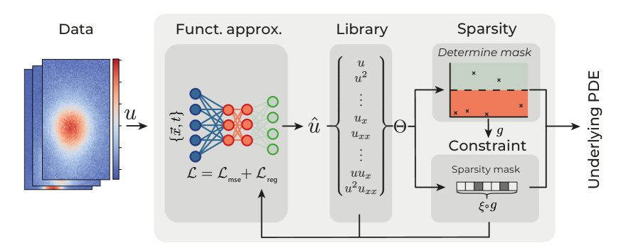
Figure 1: Schematic overview of our framework. (I) A function approximator constructs a surrogate of the data, (II) from which a Library of possible terms and the time derivative is constructed using automatic differentiation. (III) A sparsity estimator selects the active terms in the library using sparse regression and (IV) the function approximator is constrained to solutions allowed by the active terms by the constraint.

Related Work

Sparse regression

Sparse regression as a means to discover differential equations was pioneered by SINDY (Brunton, Proctor, and Kutz 2016) and PDE-find (Rudy et al. 2017). They have since been expanded to automated hyper-parameter tuning (Champion et al. 2019a; Maddu et al. 2019); a Bayesian approach for model discovery using Sparse Bayesian Learning (Yuan et al. 2019), model discovery for parametric differential equations(Rudy, Kutz, and Brunton 2019) and evolutionary approach to PDE discovery (Maslyaev, Hvatov, and Kalyuzhnaya 2019).

Deep learning-based model discovery

With the advent of Physics Informed neural networks (Raissi, Perdikaris, and Karniadakis 2017a, b), a neural network has become one of the prime approaches to create a surrogate of the data and then perform sparse regression on the networks prediction (Schaeffer 2017; Berg and Nyström 2019). Alternatively, Neural ODEs are introduced to discover unknown governing equation (Rackauckas et al. 2020) from physical data-sets. Different optimisation strategy based on the method of alternating direction is considered in (Chen, Liu, and Sun 2020), and graph based approaches have been developed recently (Seo and Liu 2019; Sanchez-Gonzalez et al. 2018). (Greydanus, Dzamba, and Yosinski 2019) and (Cranmer et al. 2020) directly encode symmetries in neural networks using respectively the Hamiltonian and Lagrangian framework. Finally, auto-encoders have been used to model PDEs and discover latent variables(Lu, Kim, and Soljačić 2019; Iten et al. 2020), but do not lead to an explicit equation and require large amounts of data.

Deep-learning based model discovery with sparse regression

Deep learning-based model discovery uses a neural network to construct a surrogate model $\hat{u}$ of the data $u$. A library of candidate terms $\Theta$ is constructed using automatic differentiation from $\hat{u}$ and the neural network is constrained to solutions allowed by this library (Both et al. 2019). The loss function of the network thus consists of two contributions, (i) a mean square error to learn the mapping $(\vec{x},t)\rightarrow\hat{u}$ and (ii) a term to constrain the network,

$$\mathcal{L}=\frac{1}{N}\sum_{i=1}^{N}\left(u_{i}-\hat{u}_{i}\right)^{2}+\frac{1}{N}\sum_{i=1}^{N}\left(\partial_{t}\hat{u}_{i}-\Theta_{i}\xi\right)^{2}.$$ (1)

The sparse coefficient vector $\xi$ is learned concurrently with the network parameters and plays two roles: 1) determining the active (i.e. non-zero) components of the underlying PDE and 2) constraining the network according to these active terms. We propose to separate these two tasks by decoupling the constraint from the sparsity selection process itself. We first calculate a sparsity mask $g$ and constrain the network only by the active terms in the mask: instead of constraining the neural network with $\xi$, we constrain it with $\xi\circ\ g$, replacing eq. 1 with

$$\mathcal{L}=\frac{1}{N}\sum_{i=1}^{N}\left(u_{i}-\hat{u}_{i}\right)^{2}+\frac{1}{N}\sum_{i=1}^{N}\left(\partial_{t}\hat{u}_{i}-\Theta_{i}(\xi\cdot g)\right)^{2}.$$ (2)

Training using eq. 2 requires two steps: first, we calculate $g$ using a sparse estimator. Next, we minimise it with respect to the network parameters using the masked coefficient vector. The sparsity mask $g$ need not be calculated differentiably, so that any classical, non-differentiable sparse estimator can be used. This approach has several additional advantages: i) It provides an unbiased estimate of the coefficient vector since we do not apply $l_{1}$ or $l_{2}$ regularisation on $\xi$, ii) the sparsity pattern is determined from the full library $\Theta$, rather than only from the remaining active terms, allowing dynamic addition and removal of active terms throughout training, and iii) we can use cross validation in the sparse estimator to find the optimal hyper parameters for model selection. Finally, we note that the sparsity mask $g$ mirrors the role of attention in transformers (Bahdanau, Cho, and Bengio 2016).

Using this change, we construct a general framework for deep learning based model discovery using four modules (see figure 1). (I) A function approximator constructs a surrogate model of the data, (II) from which a Library of possible terms and the time derivative is constructed using automatic differentiation. (III) A sparsity estimator constructs a sparsity mask to select the active terms in the library using some sparse regression algorithm and (IV) a constraint constrains the function approximator to solutions allowed by the active terms obtained from the sparsity estimator.

Training

We typically calculate the sparsity mask $g$ using an external, non-differentiable estimator. In this case, updating the mask at the right time is crucial: before the function approximator has reasonably approximated the data, updating the mask would adversely affect training, as it is likely to select the wrong terms. Vice versa, updating the mask too late risks using a function library from an overfitted network. We implement a procedure in the spirit of ”early stopping” to decide when to update: the data-set gets split into a train and test-set and we update the mask once the mean squared error on the test-set reaches a minimum or changes less than a preset value $\delta$. We typically set $\delta=10^{-6}$ to ensure the network has learned a good representation of the data.

After the first update, we periodically update the mask using the sparsity estimator. In figure 2 we demonstrate this training procedure on a Burgers equation with 1500 samples with 2$\%$ white noise. It shows the losses on the train- and testset in panel A, the coefficients of the constraint in panel B and the sparsity mask in C. In practice we observe that large data-sets with little noise typically discover the correct PDE after only a single sparsity update, but that noisy data-sets require several updates, removing only a few terms at a time. Final convergence is reached when the $l_{1}$ norm of the coefficient vector remains constant.

Package

We provide our framework as a python based package at https://github.com/PhIMaL/DeePyMoD, with the documentation and examples available at https://phimal.github.io/DeePyMoD/. Mirroring our approach, each model consists of four modules: a function approximator, library, constraint and sparsity estimator module. Each module can be customised or replaced without affecting the other modules, allowing for quick experimentation. Our framework is built on Pytorch (Paszke et al. 2019) and any Pytorch model (i.e. Recurrent Neural Networks) can be used as function approximator. The sparse estimator module follows the Scikit-learn API (Pedregosa et al. ; Buitinck et al. 2013), i.e., all the build-in Scikit-learn estimators, such as those in PySindy(de Silva et al. 2020) or SK-time (Löning et al. ), can be used.

Experiments

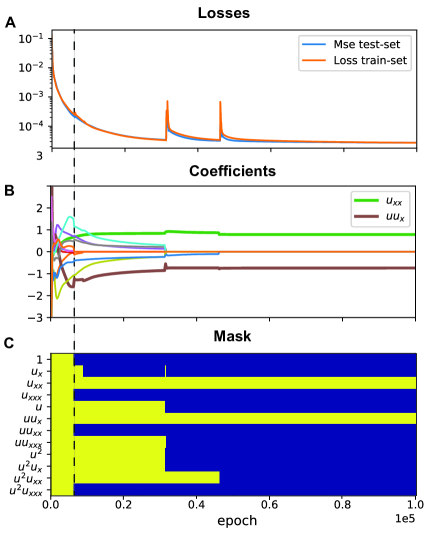
Figure 2: A) MSE of the test-set and the total loss of the train-set as function of the number of epochs. The vertical line indicates the first time the sparsity mask is applied. B) The twelve coefficients as function of the number of epochs. The two terms $u_{xx}$ and $uu_{x}$ need to be recovered. C) Dynamic sparsity mask during training. Yellow components are active, blue components are inactive.

Constraint

The sparse coefficient vector $\xi$ in eq. 1 is typically found by optimising it concurrently with the neural network parameters $\theta$. Considering a network with parameter configuration $\theta^{*}$, the problem of finding $\xi$ can be rewritten as $\operatorname*{arg\,min}_{\xi}\left|u_{t}(\theta^{*})-\Theta(\theta^{*})\xi\right|^{2}$. This can be analytically solved by least squares under mild assumptions; we calculate $\xi$ by solving this problem every iteration, rather than optimizing it using gradient descent. In figure 3 we compare the two constraining strategies on a Burgers data-set, by training for 5000 epochs without updating the sparsity mask. Panel A) shows that the least-squares approach reaches a consistently lower loss. More strikingly, we show in panel B) that the mean absolute error in the coefficients is three orders of magnitude lower. We explain the difference as a consequence of the random initialisation of $\xi$: the network is initially constrained by incorrect coefficients, prolonging convergence. The random initialisation also causes the larger spread in results compared to the least squares method. The least squares method does not suffer from sensitivity to the initialisation and consistently converges.

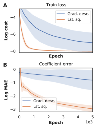
Figure 3: A) Loss and B) mean absolute error of the coefficients obtained with the gradient descent and the least squares constraint as a function of the number of epochs. Results have been averaged over twenty runs and shaded area denotes the standard deviation.

Sparsity estimator

Implementing the sparsity estimator separately from the neural network allows us to use any sparsity promoting algorithm. Here we show that a classical method for PDE model discovery, PDE-find (Rudy et al. 2017), can be used together with neural networks to perform model discovery in highly sparse and noisy data-sets. We compare it with the thresholded Lasso in figure 4 approach (Both et al. 2019) on a Burgers data-set with varying amounts of noise. The PDE-find estimator discovers the correct equation in the majority of cases, even with up to $60\%-80\%$ noise, whereas the thresholded lasso mostly fails at $40\%$. We emphasise that the modular approach we propose here allows to combine classical and deep learning-based techniques. More advanced sparsity estimators such as SR3 (Champion et al. 2019b) can easily be included in this framework.

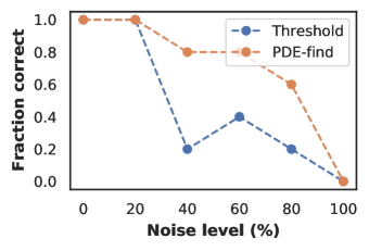
Figure 4: Fraction of correct discovered Burgers equations (averaged over 10 runs) as function of the noise level for the thresholded lasso and PDE-find sparsity estimator.

Function approximator

We show in figure 5 that a $\tanh$-based NN fails to converge on a data-set of the Kuramoto-Shivashinksy (KS) equation(panel A and B). Consequently, the coefficient vectors are incorrect (Panel D). As our framework is agnostic to the underlying function approximator, we instead use a SIREN , which is able to learn very sharp features in the underlying dynamics. In panel B we show that a SIREN is able to learn the complex dynamics of the KS equation and in panel C that it discovers the correct equation. This example shows that the choice of function approximator can be a decisive factor in the success of neural network based model discovery. Using our framework we can also explore using RNNs, Neural ODEs (Rackauckas et al. 2020) or Graph Neural Networks (Seo and Liu 2019).

Figure 5: A) Solution of the KS equation. Lower panel shows the cross section at the last time point: $t=44$. B) MSE as function of the number of epochs for both the tanh-based and SIREN NN. Coefficients as function of number of epochs for C) the SIREN. and D) the tanh-based NN. The bold curves in panel C and D are the terms in the KS equation components; green: $uu_{x}$:, blue: $u_{xx}$ and orange: $u_{xxxx}$. Only SIREN is able to discover the correct equation.

Discussion and future work

In this paper we introduced a framework for model discovery, combining classical sparsity estimation with deep learning based surrogates. Building on this, we showed that replacing the function approximator, constraint or dynamically applying the sparsity estimator during training can extend model discovery to more complex datasets, speed up convergence or make it more robust to noise. Each of the four components is decoupled from the rest and can be independently changed, making our approach a solid base for future research. Currently, the function approximator simply learns the solution using a feed forward neural network. We suspect that adding more structure, for example by using recurrent, convolutional or graph neural networks, will improve the performance of model discovery. It might also be beneficial to regularise the constraint, for example by implementing lasso or ridge regression. Updating the sparsity mask in a non-differentiable manner works because the neural network is able to learn a fairly accurate surrogate without imposing sparsity on the constraint. If the network is unable to learn an accurate representation, our approach breaks down. Updating the mask in a differentiable manner would not suffer from this drawback, and we intend to pursue this in future works.

References

- Bahdanau, Cho, and Bengio (2016) Bahdanau, D.; Cho, K.; and Bengio, Y. 2016. Neural Machine Translation by Jointly Learning to Align and Translate. arXiv:1409.0473 [cs, stat] URL http://arxiv.org/abs/1409.0473. ArXiv: 1409.0473.
- Berg and Nyström (2019) Berg, J.; and Nyström, K. 2019. Data-driven discovery of PDEs in complex datasets. Journal of Computational Physics 384: 239–252. ISSN 00219991. doi:10.1016/j.jcp.2019.01.036. URL http://arxiv.org/abs/1808.10788. ArXiv: 1808.10788.
- Both et al. (2019) Both, G.-J.; Choudhury, S.; Sens, P.; and Kusters, R. 2019. DeepMoD: Deep learning for Model Discovery in noisy data. arXiv:1904.09406 [physics, q-bio, stat] URL http://arxiv.org/abs/1904.09406. ArXiv: 1904.09406.
- Brunton, Proctor, and Kutz (2016) Brunton, S. L.; Proctor, J. L.; and Kutz, J. N. 2016. Discovering governing equations from data by sparse identification of nonlinear dynamical systems. Proceedings of the National Academy of Sciences 113(15): 3932–3937. ISSN 0027-8424, 1091-6490. doi:10.1073/pnas.1517384113. URL http://www.pnas.org/lookup/doi/10.1073/pnas.1517384113.
- Buitinck et al. (2013) Buitinck, L.; Louppe, G.; Blondel, M.; Pedregosa, F.; Mueller, A.; Grisel, O.; Niculae, V.; Prettenhofer, P.; Gramfort, A.; Grobler, J.; Layton, R.; Vanderplas, J.; Joly, A.; Holt, B.; and Varoquaux, G. 2013. API design for machine learning software: experiences from the scikit-learn project. arXiv:1309.0238 [cs] URL http://arxiv.org/abs/1309.0238. ArXiv: 1309.0238.
- Champion et al. (2019a) Champion, K.; Lusch, B.; Kutz, J. N.; and Brunton, S. L. 2019a. Data-driven discovery of coordinates and governing equations. arXiv:1904.02107 [stat] URL http://arxiv.org/abs/1904.02107. ArXiv: 1904.02107.
- Champion et al. (2019b) Champion, K.; Zheng, P.; Aravkin, A. Y.; Brunton, S. L.; and Kutz, J. N. 2019b. A unified sparse optimization framework to learn parsimonious physics-informed models from data. arXiv:1906.10612 [physics] URL http://arxiv.org/abs/1906.10612. ArXiv: 1906.10612.
- Chen, Liu, and Sun (2020) Chen, Z.; Liu, Y.; and Sun, H. 2020. Deep learning of physical laws from scarce data. arXiv:2005.03448 [physics, stat] URL http://arxiv.org/abs/2005.03448. ArXiv: 2005.03448.
- Cranmer et al. (2020) Cranmer, M.; Greydanus, S.; Hoyer, S.; Battaglia, P.; Spergel, D.; and Ho, S. 2020. Lagrangian Neural Networks. arXiv:2003.04630 [physics, stat] URL http://arxiv.org/abs/2003.04630. ArXiv: 2003.04630.
- de Silva et al. (2020) de Silva, B. M.; Champion, K.; Quade, M.; Loiseau, J.-C.; Kutz, J. N.; and Brunton, S. L. 2020. PySINDy: A Python package for the Sparse Identification of Nonlinear Dynamics from Data. arXiv:2004.08424 [physics] URL http://arxiv.org/abs/2004.08424. ArXiv: 2004.08424.
- Greydanus, Dzamba, and Yosinski (2019) Greydanus, S.; Dzamba, M.; and Yosinski, J. 2019. Hamiltonian Neural Networks. arXiv:1906.01563 [cs] URL http://arxiv.org/abs/1906.01563. ArXiv: 1906.01563.
- Harris et al. (2020) Harris, C. R.; Millman, K. J.; van der Walt, S. J.; Gommers, R.; Virtanen, P.; Cournapeau, D.; Wieser, E.; Taylor, J.; Berg, S.; Smith, N. J.; Kern, R.; Picus, M.; Hoyer, S.; van Kerkwijk, M. H.; Brett, M.; Haldane, A.; del Río, J. F.; Wiebe, M.; Peterson, P.; Gérard-Marchant, P.; Sheppard, K.; Reddy, T.; Weckesser, W.; Abbasi, H.; Gohlke, C.; and Oliphant, T. E. 2020. Array programming with NumPy. Nature 585(7825): 357–362. ISSN 0028-0836, 1476-4687. doi:10.1038/s41586-020-2649-2. URL http://www.nature.com/articles/s41586-020-2649-2.
- Hunter (2007) Hunter, J. D. 2007. Matplotlib: A 2D Graphics Environment. Computing in Science Engineering 9(3): 90–95. ISSN 1558-366X. doi:10.1109/MCSE.2007.55. Conference Name: Computing in Science Engineering.
- Iten et al. (2020) Iten, R.; Metger, T.; Wilming, H.; del Rio, L.; and Renner, R. 2020. Discovering physical concepts with neural networks. Physical Review Letters 124(1): 010508. ISSN 0031-9007, 1079-7114. doi:10.1103/PhysRevLett.124.010508. URL http://arxiv.org/abs/1807.10300. ArXiv: 1807.10300.
- Lu, Kim, and Soljačić (2019) Lu, P. Y.; Kim, S.; and Soljačić, M. 2019. Extracting Interpretable Physical Parameters from Spatiotemporal Systems using Unsupervised Learning. arXiv:1907.06011 [physics, stat] URL http://arxiv.org/abs/1907.06011. ArXiv: 1907.06011.
- (16) Löning, M.; Bagnall, A.; Ganesh, S.; and Kazakov, V. ???? sktime: A Unified Interface for Machine Learning with Time Series 10.
- Maddu et al. (2019) Maddu, S.; Cheeseman, B. L.; Sbalzarini, I. F.; and Müller, C. L. 2019. Stability selection enables robust learning of partial differential equations from limited noisy data. arXiv:1907.07810 [physics] URL http://arxiv.org/abs/1907.07810. ArXiv: 1907.07810.
- Maslyaev, Hvatov, and Kalyuzhnaya (2019) Maslyaev, M.; Hvatov, A.; and Kalyuzhnaya, A. 2019. Data-driven PDE discovery with evolutionary approach. arXiv:1903.08011 [cs, math] 11540: 635–641. doi:10.1007/978-3-030-22750-0˙61. URL http://arxiv.org/abs/1903.08011. ArXiv: 1903.08011.
- Paszke et al. (2019) Paszke, A.; Gross, S.; Massa, F.; Lerer, A.; Bradbury, J.; Chanan, G.; Killeen, T.; Lin, Z.; Gimelshein, N.; Antiga, L.; Desmaison, A.; Köpf, A.; Yang, E.; DeVito, Z.; Raison, M.; Tejani, A.; Chilamkurthy, S.; Steiner, B.; Fang, L.; Bai, J.; and Chintala, S. 2019. PyTorch: An Imperative Style, High-Performance Deep Learning Library. arXiv:1912.01703 [cs, stat] URL http://arxiv.org/abs/1912.01703. ArXiv: 1912.01703.
- (20) Pedregosa, F.; Varoquaux, G.; Gramfort, A.; Michel, V.; Thirion, B.; Grisel, O.; Blondel, M.; Prettenhofer, P.; Weiss, R.; Dubourg, V.; Vanderplas, J.; Passos, A.; and Cournapeau, D. ???? Scikit-learn: Machine Learning in Python. MACHINE LEARNING IN PYTHON 6.
- Perez and Granger (2007) Perez, F.; and Granger, B. E. 2007. IPython: A System for Interactive Scientific Computing. Computing in Science Engineering 9(3): 21–29. ISSN 1558-366X. doi:10.1109/MCSE.2007.53.
- Rackauckas et al. (2020) Rackauckas, C.; Ma, Y.; Martensen, J.; Warner, C.; Zubov, K.; Supekar, R.; Skinner, D.; and Ramadhan, A. 2020. Universal Differential Equations for Scientific Machine Learning. arXiv:2001.04385 [cs, math, q-bio, stat] URL http://arxiv.org/abs/2001.04385. ArXiv: 2001.04385.
- Raissi, Perdikaris, and Karniadakis (2017a) Raissi, M.; Perdikaris, P.; and Karniadakis, G. E. 2017a. Physics Informed Deep Learning (Part I): Data-driven Solutions of Nonlinear Partial Differential Equations. arXiv:1711.10561 [cs, math, stat] URL http://arxiv.org/abs/1711.10561. ArXiv: 1711.10561.
- Raissi, Perdikaris, and Karniadakis (2017b) Raissi, M.; Perdikaris, P.; and Karniadakis, G. E. 2017b. Physics Informed Deep Learning (Part II): Data-driven Discovery of Nonlinear Partial Differential Equations. arXiv:1711.10566 [cs, math, stat] URL http://arxiv.org/abs/1711.10566. ArXiv: 1711.10566.
- Rudy et al. (2017) Rudy, S. H.; Brunton, S. L.; Proctor, J. L.; and Kutz, J. N. 2017. Data-driven discovery of partial differential equations. Science Advances 3(4): e1602614. ISSN 2375-2548. doi:10.1126/sciadv.1602614. URL http://advances.sciencemag.org/lookup/doi/10.1126/sciadv.1602614.
- Rudy, Kutz, and Brunton (2019) Rudy, S. H.; Kutz, J. N.; and Brunton, S. L. 2019. Deep learning of dynamics and signal-noise decomposition with time-stepping constraints. Journal of Computational Physics 396: 483–506. ISSN 00219991. doi:10.1016/j.jcp.2019.06.056. URL http://arxiv.org/abs/1808.02578. ArXiv: 1808.02578.
- Sanchez-Gonzalez et al. (2018) Sanchez-Gonzalez, A.; Heess, N.; Springenberg, J. T.; Merel, J.; Riedmiller, M.; Hadsell, R.; and Battaglia, P. 2018. Graph networks as learnable physics engines for inference and control. arXiv:1806.01242 [cs, stat] URL http://arxiv.org/abs/1806.01242. ArXiv: 1806.01242.
- Schaeffer (2017) Schaeffer, H. 2017. Learning partial differential equations via data discovery and sparse optimization. Proceedings of the Royal Society A: Mathematical, Physical and Engineering Sciences 473(2197): 20160446. ISSN 1364-5021, 1471-2946. doi:10.1098/rspa.2016.0446. URL https://royalsocietypublishing.org/doi/10.1098/rspa.2016.0446.
- Seo and Liu (2019) Seo, S.; and Liu, Y. 2019. Differentiable Physics-informed Graph Networks. arXiv:1902.02950 [cs, stat] URL http://arxiv.org/abs/1902.02950. ArXiv: 1902.02950.
- Sitzmann et al. (2020) Sitzmann, V.; Martel, J. N. P.; Bergman, A. W.; Lindell, D. B.; and Wetzstein, G. 2020. Implicit Neural Representations with Periodic Activation Functions. arXiv:2006.09661 [cs, eess] URL http://arxiv.org/abs/2006.09661. ArXiv: 2006.09661.
- Virtanen et al. (2020) Virtanen, P.; Gommers, R.; Oliphant, T. E.; Haberland, M.; Reddy, T.; Cournapeau, D.; Burovski, E.; Peterson, P.; Weckesser, W.; Bright, J.; van der Walt, S. J.; Brett, M.; Wilson, J.; Millman, K. J.; Mayorov, N.; Nelson, A. R. J.; Jones, E.; Kern, R.; Larson, E.; Carey, C. J.; Polat, .; Feng, Y.; Moore, E. W.; VanderPlas, J.; Laxalde, D.; Perktold, J.; Cimrman, R.; Henriksen, I.; Quintero, E. A.; Harris, C. R.; Archibald, A. M.; Ribeiro, A. H.; Pedregosa, F.; van Mulbregt, P.; and Contributors, S. . . 2020. SciPy 1.0–Fundamental Algorithms for Scientific Computing in Python. Nature Methods 17(3): 261–272. ISSN 1548-7091, 1548-7105. doi:10.1038/s41592-019-0686-2. URL http://arxiv.org/abs/1907.10121. ArXiv: 1907.10121.
- Yuan et al. (2019) Yuan, Y.; Li, J.; Li, L.; Jiang, F.; Tang, X.; Zhang, F.; Liu, S.; Goncalves, J.; Voss, H. U.; Li, X.; Kurths, J.; and Ding, H. 2019. Machine Discovery of Partial Differential Equations from Spatiotemporal Data. arXiv:1909.06730 [physics, stat] URL http://arxiv.org/abs/1909.06730. ArXiv: 1909.06730.