Certification of non-Gaussian states with operational measurements

Abstract

We derive a theoretical framework for the experimental certification of non-Gaussian features of quantum states using double homodyne detection. We rank experimental non-Gaussian states according to the recently defined stellar hierarchy and we propose practical Wigner negativity witnesses. We simulate various use-cases ranging from fidelity estimation to witnessing Wigner negativity. Moreover, we extend results on the robustness of the stellar hierarchy of non-Gaussian states. Our results illustrate the usefulness of double homodyne detection as a practical measurement scheme for retrieving information about continuous variable quantum states.

I Introduction

Recent years have witnessed many developments that are paving the road towards quantum technologies Monz et al. (2016); Wang et al. (2019); Arute et al. (2019); Jurcevic et al. (2020). The physical backbone of these advances often relies on the discrete nature of certain quantum observables, known as the discrete-variable (DV) approach. In contrast, one can also develop quantum technologies based on systems that have a phase space representation, which leads to quantum observables with a continuum of possible measurement outcomes Braunstein and van Loock (2005); Pfister (2019); Bourassa et al. (2020). This continuous-variable (CV) approach has gradually made its way to the forefront in the development of quantum information protocols by the experimental realisations of large entangled cluster states in optical setups Larsen et al. (2019); Asavanant et al. (2019), and quantum error correction in superconducting circuits Campagne-Ibarcq et al. (2020).

CV quantum states are represented in phase space using quasiprobability distributions Cahill and Glauber (1969), such as Glauber-Sudarshan, Wigner, or Husimi functions. Quantum states are then split into two main categories according to the shape of their representation in phase space: Gaussian states and non-Gaussian states. In CV quantum optics, Gaussian states and processes are well understood and routinely produced and processed experimentally, the deterministic preparation of highly entangled states over a large number of modes being a striking example of what they enable Su et al. (2012); Roslund et al. (2014); Chen et al. (2014); Yoshikawa et al. (2016). These states and processes also feature an elegant theoretical description with the symplectic formalism Weedbrook et al. (2012). However, their non-Gaussian counterparts are necessary for a large variety of quantum information processing tasks Bartlett et al. (2002); Mari and Eisert (2012); Rahimi-Keshari et al. (2016).

Non-Gaussian states come in many varieties and can have a wide range of properties. The most benign members of this class of states are non-Gaussian mixtures of Gaussian states, which are generally not considered to be of interest for quantum information procession, because they can still be efficiently simulated via classical computers. Another important class of states are those with non-positive Wigner functions, which are required to reach a quantum computational advantage Mari and Eisert (2012). One can also find states with a positive Wigner function that cannot be written as a mixture of Gaussian states Filip and Mišta Jr (2011), these are sometimes referred to as quantum non-Gaussian states Genoni et al. (2013). However, these classes are still crude, containing states with widely different properties in their phase-space representation and that are still hard to classify in term of usefulness in quantum protocols.

To further explore the structure of CV quantum states in the single-mode-case the stellar hierarchy Chabaud et al. (2020a) was introduced, where each level corresponds to the number of single-photon additions necessary to engineer the states, together with Gaussian unitary operations.

Such non-Gaussian features in CV quantum states are not only challenging to produce experimentally, they are also difficult to detect. Homodyne tomography Lvovsky and Raymer (2009); Tiunov et al. (2020), based on maximum-likelihood estimation, is a common tool in quantum optics to reconstruct the full quantum state, thus allowing to extract arbitrary features. However, when implementing this method the number of required measurements grows exponentially with the number of modes. Therefore, it is often more interesting to use a benchmark for the desired properties of the state Eisert et al. (2019), rather than performing a full state tomography. A natural additional requirement for such a benchmark is an accompanying confidence interval, which is, again, hard to extract from maximum-likelihood tomography Silva et al. (2017); Blume-Kohout (2010); Faist and Renner (2016). Machine learning methods have successfully been applied to benchmark the Wigner-negativity of highly multimode states Cimini et al. (2020), but these methods are most fruitful when good training data are available. In other words, a machine learning algorithm can only recognize the features of a state when it has seen many similar states before.

In this Manuscript, we provide a complementary approach for certifying the presence of certain features of quantum states, based on double homodyne detection Paris (1996a); Ferraro et al. (2005). This detection scheme is directly connected to the $Q$ function, which can be exploited for retrieving information about continuous variable quantum states Chabaud et al. (2019) and for the verification of Boson Sampling output states Aaronson and Arkhipov (2013); Chabaud et al. (2020b). Here we will use the techniques of Chabaud et al. (2019) to estimate quantum state fidelity, and from these estimates we produce a robust benchmark for the stellar rank of the state. This allows us to operationally identify the number of single-photon additions applied on a Gaussian states that is necessary to reach a given fidelity with a given quantum state. Furthermore, we can use the same techniques to construct witnesses for Wigner negativity. By simulating outcomes for double homodyne detection for realistic states (some of which were reconstructed from experimental data), we explore the experimental feasibility of this protocol. We show that with a realistic amount of loss and an achievable number of measurements, we can extract stellar rank and Wigner-negativity with a high degree of confidence.

II Retrieving information via phase space

II.1 Phase space measurements

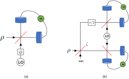
Figure 1: Phase space measurements. (a) Homodyne detection of the rotated quadrature $\hat{x}_{\phi}$. (b) Double homodyne detection with unbalancing parameter $\zeta$. The dashed red lines represent beam splitters and LO stands for Local Oscillator, i.e., a strong coherent state.

Homodyne detection is the most widely used experimental procedure to perform quadrature measurements on an optical state. As described in (Fig. 1(a)), it consists in mixing the state to be measured on a balanced beam splitter with a reference field, and compute the difference between intensity measurements on both outputs. Depending on the relative phase $\phi$ between the fields, it yields the sampling of the quadrature observable $\hat{x}_{\phi}=\cos\phi\,\hat{q}+\sin\phi\,\hat{p}$.

Provided many copies of a state are available, performing optical homodyne detection allows for the reconstruction of the Wigner function of the state. This quantum state tomography requires many measurement settings, one for each value of $\phi$, and to solve a complex inverse problem Lvovsky and Raymer (2009). In practice, a discrete set of angles is chosen, introducing errors in the reconstruction procedure.

Double homodyne detection, sometimes called heterodyne or eight-port homodyne detection Ferraro et al. (2005), consists in measuring both quadratures of a single-mode state $\rho$. This is achieved by splitting the state on a beam splitter and performing two homodyne detections, one on each output with a $\pi/2$ phase shift between them (Fig. 1(b)). Double homodyne detection yields a complex outcome, whose real and imaginary parts are respectively both outcomes of the measurements, and projects the measured state onto a coherent state. Hence, it leads to the sampling of the Husimi $Q$ function of the state, defined as

$$Q_{\rho}(\alpha)=\frac{1}{\pi}\braket{\alpha}{\rho}{\alpha},$$ (1)

for all $\alpha\in\mathbb{C}$, where $\ket{\alpha}$ is the coherent state of amplitude $\alpha$. Note that when the first beam splitter is unbalanced, the double homodyne detection is also unbalanced and projects the measured state onto a finitely squeezed coherent state instead of a coherent state, whose squeezing parameter depends on the unbalancing. In the limit of infinite squeezing, i.e., with a reflectivity of $0$ or $1$ for the input beamsplitter, one retrieves the homodyne detection setup.

Provided many copies of a state are available, optical double homodyne detection allows one to perform continuous variable quantum state tomography with a single measurement setting, since varying the phase of the local oscillator is no longer needed. This is because the Husimi function is directly sampled with double homodyne detection and it contains all the information about the state, whereas for homodyne detection the Wigner function contains all the information about the state but it cannot be sampled directly—it is not a probability density in general—and its marginals are sampled instead.

While being slightly more complicated experimentally than homodyne detection, double homodyne detection has the advantage of providing a reliable tomographic recovery with a single measurement setting Chabaud et al. (2019). The POVM element for unbalanced double homodyne detection with outcome $\alpha\in\mathbb{C}$ is given by

$$\Pi_{\alpha}=\frac{1}{\pi}\ket{\alpha,\zeta}\!\bra{\alpha,\zeta},$$ (2)

where $\ket{\alpha,\zeta}=\hat{S}(\zeta)\hat{D}(\alpha)\ket{0}$ is a squeezed coherent state, with $\hat{D}(\alpha)=e^{\alpha\hat{a}^{\dagger}-\alpha^{*}\hat{a}}$ and $\hat{S}(\zeta)=e^{\frac{1}{2}(\zeta\hat{a}^{2}-\zeta^{*}\hat{a}^{{\dagger}2})}$, whose squeezing parameter $\zeta$ depends on the unbalanced double homodyne detection setup. For reflectance $R$ and transmitance $T$ of the beam splitter, we have $|\zeta|=|\log(\frac{R}{T})|$ and the phase of $\zeta$ is given by the phase of the local oscillator Chabaud et al. (2017).

In particular, unbalanced double homodyne detection is formally equivalent to a squeezing operation followed by a balanced double homodyne detection. Similarly, since the double homodyne POVM elements are projectors onto coherent states, a displacement before a double homodyne detection can be reverted by translating the classical samples by the amplitude of the displacement. This implies that any single-mode Gaussian unitary operation can be reverted at the level of the measurement by playing with the unbalancing of the detection and by translating the classical samples Weedbrook et al. (2012).

II.2 Reliable expectation value estimation with double homodyne detection

A reliable quantum state certification method with double homodyne detection has been introduced in Chabaud et al. (2019), and recently enhanced in Chabaud et al. (2020b) to allow for the efficient verification of Boson Sampling output states Aaronson and Arkhipov (2013). Using samples from balanced double homodyne detection of various copies of an experimental (mixed) state $\rho$, this method provides reliable estimates of the expectation value $\,\mathrm{Tr}(\hat{A}\rho)$, for any target single-mode operator $\hat{A}$ with bounded support over the Fock basis. Choosing $\hat{A}=\ket{l}\!\bra{k}$, one may estimate the density matrix element $\rho_{kl}=\,\mathrm{Tr}(\ket{l}\!\bra{k}\rho)$ in Fock basis and perform a full reconstruction by varying $k$ and $l$. Alternatively, choosing $\hat{A}=\ket{C}\!\bra{C}$, where $\ket{C}$ is a core state Menzies and Filip (2009); Chabaud et al. (2020a), i.e., a normalised pure state with bounded support over the Fock basis, one may estimate the fidelity $F(C,\rho)=\,\mathrm{Tr}(\ket{C}\!\bra{C}\rho)$.

Moreover, since any single-mode Gaussian unitary operation before double homodyne detection can be reverted by unbalancing the detection and translating the classical samples, this also allows for the estimation of expectation values of operators of the form $\hat{G}\hat{A}\hat{G}^{\dagger}$, where $\hat{G}$ is a Gaussian unitary operation and $\hat{A}$ is an operator with bounded support over the Fock basis.

This certification method provides analytical confidence intervals for the estimation and makes minimal assumptions on the state preparation: unlike previous existing methods Paris (1996b, a), it does not assume that the measured state $\rho$ has a bounded support over the Fock basis. This is especially important for the certification of non-Gaussian features, given that such an assumption may induce non-Gaussianity (applying a cutoff in Fock basis to, e.g., a coherent state with nonzero amplitude always makes it non-Gaussian). We further assume that identical and identically distributed copies of the measured state $\rho$ are available, but a refined version of the protocol without this assumption is possible Chabaud et al. (2019).

Let us now describe how to estimate the expectation value of a target operator $\hat{A}=\sum_{k,l}{A_{kl}\ket{k}\!\bra{l}}$, with bounded support over the Fock basis, given a confidence parameter $\delta>0$ Chabaud et al. (2019, 2020b). Considering $N$ copies of the unknown (mixed) quantum state $\rho$, $N$ double homodyne detection are performed leading to the measurement results $\alpha_{1},\dots,\alpha_{N}\in\mathbb{C}$. One then compute the estimate $F_{\hat{A}}(\alpha_{1},\dots,\alpha_{N})$, which is defined as the mean over these measurements of an expectation value estimator whose expression is detailed in Appendix A. The estimate $F_{\hat{A}}(\alpha_{1},\dots,\alpha_{N})$ obtained is $\epsilon$-close to the expectation value $\,\mathrm{Tr}(\hat{A}\rho)$ with probability greater than $1-\delta$, for a number of samples $N=\mathcal{O}(\frac{1}{\epsilon^{2+t}}\log{\frac{1}{\delta}})$, where the prefactor depends on a free parameter $t>0$. This protocol features several free parameters which may be optimised, and we refer to Appendix A for a detailed analysis of the protocol and its optimisation.

In what follows, we consider applications of this protocol beyond quantum state tomography, for probing non-Gaussian properties of continuous variable quantum states:

• Ranking non-Gaussian states (section III): due to the robustness of the stellar hierarchy of quantum states Chabaud et al. (2020a), fidelity estimators with non-Gaussian states provide witnesses for the stellar rank. The expectation value estimation protocol yields such fidelity estimators with reliable confidence intervals. We generalise various results of Chabaud et al. (2020a) for the robustness of the stellar hierarchy, and illustrate our results with numerical simulations.

• Witnessing Wigner negativity (section IV): since the Wigner function is related to expectation values of displaced parity operators, we obtain witnesses for the negativity of the Wigner function using the double homodyne expectation value estimation protocol.

III Ranking non-Gaussian states

A pure state is non-Gaussian if and only if it is orthogonal to a coherent state, which equivalently means that its Husimi $Q$ function (1) has zeros Lütkenhaus and Barnett (1995). We denote by $\mathcal{H}_{\infty}$ the single-mode infinite-dimensional Hilbert space. The stellar rank $r^{\star}(\psi)$ of a pure single-mode normalised quantum state $\ket{\psi}\in\mathcal{H}_{\infty}$ has been defined in Chabaud et al. (2020a) as the number of zeros of its Husimi function (counted with half multiplicity), where it was shown that it corresponds to the minimal number of photon additions needed to engineer the state from the vacuum, together with Gaussian unitary operations (Fig. 2). We write $\overline{\mathbb{N}}=\mathbb{N}\cup\{+\infty\}$, with the convention $n<+\infty\Leftrightarrow n\in\mathbb{N}$. States of zero stellar rank thus are pure Gaussian states and the stellar rank is either finite or infinite. States having infinite stellar rank include cat states and GKP states (for the latter, the Husimi function has an infinite number of zeros since it is quasiperiodic and GKP states are non-Gaussian).

For a mixed state $\rho$, this definition is generalised to

$$r^{\star}(\rho)=\inf_{\{p_{i},\psi_{i}\}}{\sup_{i}{\,r^{\star}(\psi_{i})}},$$ (3)

where the infimum is taken over the statistical ensembles $\{p_{i},\psi_{i}\}$ such that $\rho=\sum_{i}{p_{i}\ket{\psi_{i}}\bra{\psi_{i}}}$. In particular, a mixed state has a nonzero stellar rank if it cannot be expressed as a mixture of pure Gaussian states, i.e., when it is quantum non-Gaussian Genoni et al. (2013).

III.1 Stellar hierarchy of non-Gaussian states

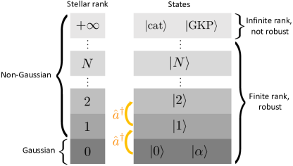
Figure 2: A pictorial depiction of the stellar hierarchy. The right column gives examples of pure states of each stellar rank, which corresponds to the minimal number of photon additions $\hat{a}^{\dagger}$ necessary to obtain the state from the vacuum. All states of finite stellar rank are robust, i.e., they only have states of equal or higher stellar rank in their close vicinity.

The stellar rank induces a hierarchy among normalised quantum states in $\mathcal{H}_{\infty}$, the so-called stellar hierarchy.

Pure states of finite stellar rank in the hierarchy may be obtained from a core state, i.e., a state with finite support over the Fock basis, with a Gaussian unitary operation Chabaud et al. (2020a). Since single-mode Gaussian unitary operations can be decomposed as a squeezing and a displacement Weedbrook et al. (2012), pure states of stellar rank $n\in\mathbb{N}$ are of the form

$$\hat{S}(\xi)\hat{D}(\alpha)\sum_{m=0}^{n}{c_{m}\ket{m}},$$ (4)

where $\xi,\alpha\in\mathbb{C}$, $c_{n}\neq 0$ and $\sum_{m=0}^{n}{|c_{m}|^{2}=1}$. Equivalently, these states may be obtained from the vacuum using $n$ single-photon additions together with Gaussian unitary operations. We show in Appendix B that a single-photon subtraction may only increase the stellar rank by at most $1$. This implies that such a state cannot be engineered with less than $n$ single-photon additions and/or subtractions, together with Gaussian unitary operations.

Hereafter, we show how to certify the nonzero stellar ranks of an experimental (mixed) quantum state using fidelity estimation with a target pure state. To that end, we derive robustness properties of the stellar hierarchy and introduce fidelity-based witnesses for the stellar rank.

The stellar robustness $R^{\star}(\psi)$ of a state $\ket{\psi}\in\mathcal{H}_{\infty}$ corresponds to the amount of deviation in trace distance from $\ket{\psi}$ which is necessary to reach states of lower stellar rank Chabaud et al. (2020a). In order to probe the stellar hierarchy with phase space measurements, we introduce the following definition, which generalises the notion of stellar robustness:

Definition 1 ($k$-robustness).

Let $\ket{\psi}\in\mathcal{H}_{\infty}$. For all $k\in\overline{\mathbb{N}}^{*}$, the $k$-robustness of the state $\ket{\psi}$ is defined as

$$R^{\star}_{k}(\psi)\stackrel{{\scriptstyle\mathrm{def}}}{{=}}\smashoperator[]{\inf_{r^{\star}(\phi)<k}^{}}{D(\phi,\psi)},$$ (5)

where $D(\phi,\psi)=\sqrt{1-|\braket{\phi}{\psi}|^{2}}$ denotes the trace distance and where the infimum is over all states $\ket{\phi}\in\mathcal{H}_{\infty}$ with a stellar rank lower than $k$.

For all $k\in\mathbb{N}^{*}$, the $k$-robustness $R^{\star}_{k}$ quantifies how much one has to deviate from a quantum state in trace distance to find another quantum state which has a stellar rank between $0$ and $k-1$. When $k=+\infty$, the $\infty$-robustness quantifies how much one has to deviate from a quantum state in trace distance to find another quantum state of finite stellar rank. Note that for $k=r^{\star}(\psi)$ we recover the stellar robustness.

The stellar robustness $R^{\star}$ of a state $\ket{\psi}$ satisfies Chabaud et al. (2020a):

$$\smashoperator[]{\sup_{r^{\star}(\rho)<r^{\star}(\psi)}^{}}{F(\rho,\psi)}=1-[R^{\star}(\psi)]^{2},$$ (6)

where $F(\rho,\psi)=\braket{\psi}{\rho}{\psi}$ is the fidelity. Certifying that an experimental (mixed) state $\rho$ has a fidelity greater than $1-[R^{\star}(\psi)]^{2}$ with a given target pure state $\ket{\psi}$ thus ensures that the state $\rho$ has stellar rank equal or greater than $r^{\star}(\psi)$. A similar property holds for the $k$-robustness:

$$\smashoperator[]{\sup_{r^{\star}(\rho)<k}^{}}F(\rho,\psi)=1-[R_{k}^{\star}(\psi)]^{2}.$$ (7)

We refer to Appendix C for a short proof. Certifying that an experimental (mixed) state $\rho$ has a fidelity greater than $1-[R^{\star}_{k}(\psi)]^{2}$ with a given target pure state $\ket{\psi}$ thus ensures that the state $\rho$ has stellar rank greater or equal to $k$. This implies that such a state cannot be engineered with less than $k$ single-photon additions and/or subtractions, together with Gaussian unitary operations. In particular, the fidelity of an experimental state with any non-Gaussian target state $\ket{\psi}$ such that $R_{k}^{\star}(\psi)>0$ can serve as a witness for a stellar rank $k$, i.e., as a certificate that the experimental state has a stellar rank no less that $k$.

Given a target state $\ket{\psi}$ of stellar rank $r^{\star}(\psi)$, let us detail when $R_{k}^{\star}(\psi)>0$. The robustness of the stellar hierarchy Chabaud et al. (2020a) implies that each state of a given finite stellar rank is isolated from all the lower stellar ranks. On the other hand, no state of a given finite stellar rank is isolated from any equal or higher stellar rank. That is, for any finite-rank state $\ket{\psi}\in\mathcal{H}_{\infty}$, $R_{k}^{\star}(\psi)>0$ when $k\leq r^{\star}(\psi)$, whereas $R_{k}^{\star}(\psi)=0$ for $k>r^{\star}(\psi)$. Furthermore, states of infinite stellar rank are not isolated from lower stellar ranks, unlike states of finite stellar rank. Any state of infinite can therefore be approximated arbitrarily well by finite-rank states. However, these approximations will always come with a finite error, since states of infinite stellar rank are isolated from states of bounded stellar rank. That is, for states $\ket{\psi}$ of infinite rank, we find that $R_{k}^{\star}(\psi)>0$ for all finite values of $k$, and $R_{k}^{\star}(\psi)=0$ for $k=\infty$.

Hence, with Eq. (7) the fidelity with any target pure state of a given stellar rank may serve as a witness for any lower stellar rank. This raises the question of how to compute the value of the maximum achievable fidelity with a given target state using states of finite stellar rank less than $k$ (or equivalently its $k$-robustness), for $k\in\mathbb{N}^{*}$. In Chabaud et al. (2020a), it was shown how to obtain such quantities with a numerical optimisation. However, the number of parameters in the optimisation had to grow with $k$, making the optimisation rapidly impractical. Hereafter, we show that the maximum achievable fidelities can be obtained with an optimisation over two complex parameters only.

Let us define, for all $n\in\mathbb{N}$,

$$\Pi_{n}=\sum_{m=0}^{n}{\ket{m}\!\bra{m}},$$ (8)

the projector onto the subspace of $\mathcal{H}_{\infty}$ spanned by the Fock states $\ket{0},\dots,\ket{n}$.

Theorem 1.

Let $k\in\mathbb{N}^{*}$ and let $\ket{\psi}\in\mathcal{H}_{\infty}$. Then, the maximum achievable fidelity with the target state $\ket{\psi}$ using states of finite stellar rank less than $k$ is given by

$$\smashoperator[]{\sup_{r^{\star}(\rho)<k}^{}}F(\rho,\psi)=\sup_{\hat{G}\in\mathcal{G}}{\,\mathrm{Tr}\left[\Pi_{k-1}\hat{G}\ket{\psi}\!\bra{\psi}\hat{G}^{\dagger}\right]},$$ (9)

where the supremum is over Gaussian unitary operations. Moreover, assuming the optimisation yields a Gaussian operation $\hat{G}_{0}$, an optimal approximating state is

$$\hat{G}_{0}^{\dagger}\left(\frac{\Pi_{k-1}\hat{G}_{0}\ket{\psi}}{\left\|\Pi_{k-1}\hat{G}_{0}\ket{\psi}\right\|}\right)\!\!.$$ (10)

We refer to Appendix D for a detailed proof. Since single-mode Gaussian unitary operations can be decomposed as a squeezing and a displacement, the optimisation is over two complex parameters only, corresponding to this squeezing and this displacement.

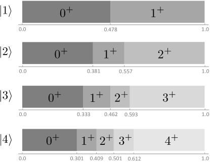
Figure 3: Achievable fidelities with target Fock states $\ket{1}$, $\ket{2}$, $\ket{3}$ and $\ket{4}$, using states of finite stellar rank. In each fidelity region, the number indicates the minimal stellar rank of states achieving these fidelities, i.e., it corresponds to the minimal number of photon additions and/or subtractions needed to build these states, together with Gaussian operations.

In order to obtain an intuitive graphical representation we introduce the following definition:

Definition 2.

The profile of achievable fidelities with a non-Gaussian target pure state is defined as the set of achievable fidelities with this state using states of finite stellar rank $k$, for each $k\in\mathbb{N}^{*}$.

This definition corresponds to the task of engineering an approximation of a target pure state using a finite number of photon additions and/or subtractions, together with Gaussian unitary operations. For each stellar rank, if $\sigma$ denotes a state for which the maximum fidelity is achieved, then any lower fidelity may also be obtained by considering the states $\rho_{p}=p\ket{\perp}\bra{\perp}+(1-p)\sigma$, for $0\leq p<1$, where $\ket{\perp}$ is a coherent state orthogonal to the target state (which exists when the target state is non-Gaussian, i.e., its Husimi function has zeros). In the following, we derive several profiles of achievable fidelities for specific target non-Gaussian states, using Theorem 1 (see Fig. 3).

Note that applying a Gaussian unitary operation to the target state yields a state which has the same profile of achievable fidelities, since the $k$-robustness is invariant under these operations. Hence, one may optimise the choice of target state over all Gaussian unitary operations in order to maximise the fidelity of the experimental state with the target state, before making use of the profile of achievable fidelities. In particular, photon-subtracted squeezed states and photon-added squeezed states have the same profile of achievable fidelities as the single-photon Fock state, since they are Gaussian-convertible to that state, i.e., they are related to that state by Gaussian unitary operations Chabaud et al. (2020a).

III.2 Fock states

Let us now consider the example of target core states and Fock states in particular. Using Theorem 1, we have obtained numerically the maximum achievable fidelities with a target core state $\cos\phi\ket{0}+e^{i\chi}\sin\phi\ket{1}$ of stellar rank $1$ using states of stellar rank $0$, i.e., Gaussian states (see Appendix E.1). We find that the most robust state of stellar rank $1$ is the single-photon Fock state $\ket{1}$ (and all the states of the form $\hat{G}\ket{1}$, where $\hat{G}$ is a Gaussian unitary operation).

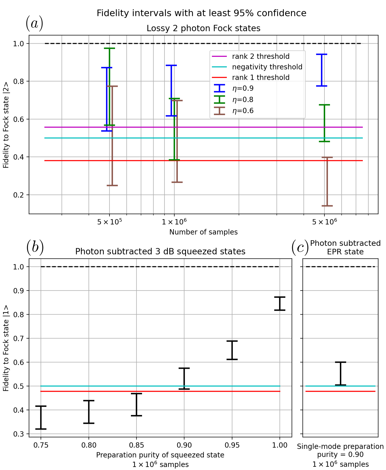
Figure 4: Estimation of fidelity with target Fock states at 95% confidence, using simulated samples from double homodyne detection of various states. The precision of the estimate varies depending on the number of samples used. We display the stellar rank 1 (resp. 2) threshold in red (resp. purple) and the Wigner negativity witness threshold (see section IV) in cyan. Note that the rank $1$ threshold varies depending on whether the target state is the Fock state $\ket{1}$ or $\ket{2}$, as can be checked with Fig. 3. (a) Lossy 2 photon Fock states $(1-\eta)^{2}|0\rangle\langle 0|+2\eta(1-\eta)|1\rangle\langle 1|+\eta^{2}|2\rangle\langle 2|$, where $\eta$ is an efficiency parameter, and target Fock state $\ket{2}$. For $\eta=0.9$, $0.8$ and $0.6$, the true fidelities to $|2\rangle$ are $0.81$, $0.64$ and $0.36$, respectively. The Wigner negativity threshold is obtained numerically. (b) Photon-subtracted squeezed vacuum states with $3$dB of squeezing and target Fock state $\ket{1}$, for several values of the preparation purity, i.e., the purity of the squeezed vacuum state before the photon subtraction. (c) A photon subtracted two-mode EPR state with experimental covariance matrix taken from Ra et al. (2020) and target Fock state $\ket{1}$. Simulated photon subtraction is done on the first mode and double homodyne measurement on the second mode of the EPR state.

The maximum achievable fidelity with a single-photon Fock state $\ket{1}$ using states of stellar rank $0$, i.e., Gaussian states, is given by $3\sqrt{3}/(4e)\approx 0.478$ Chabaud et al. (2020a). Using Theorem 1, we have obtained numerically the profiles of achievable fidelities for Fock states $\ket{2}$, $\ket{3}$, $\ket{4}$ (see Appendix E.2), depicted in Fig. 3.

These profiles indicate the stellar rank necessary to achieve any fidelity with these Fock states. In particular, the fidelity between an experimental state and a target Fock state can serve as a witness for the stellar rank of the experimental state. For example, we see with Fig. 3 that no state of stellar rank less or equal to $1$ can achieve a fidelity greater than $0.5$ with the Fock state $\ket{3}$. Hence, if the fidelity of an experimental state with the Fock state $\ket{3}$ is greater than $0.5$, then it has a stellar rank greater or equal to $2$, implying that it could not have been produced by less than two photon additions or subtractions, together with Gaussian unitary operations.

In order to illustrate the practicality of these fidelity-based witnesses for the stellar rank, we have simulated the double homodyne expectation value estimation from section II.2 for various states (see Fig. 4). To do so, we computed their $Q$ function and performed rejection sampling to simulate the detection. Then, we estimated their fidelity with target Fock states at 95% confidence using the simulated samples, thus obtaining witnesses for their stellar rank. For further details on the simulation procedure, see Appendix A. When the lower bound of the confidence interval is greater than a given threshold, one can certify at 95% confidence the corresponding property, e.g., a stellar rank greater or equal to $1$ or $2$. Note that for Fig. 4 (c), the $Q$ function of the photon subtracted two-mode EPR state is computed from an experimental covariance matrix acquired in Ra et al. (2020), where actual measurements of such state display Wigner negativity. Additionally, we have also represented a threshold for the certification of Wigner negativity using a similar witness, as detailed in the next section.

IV Wigner negativity

In the previous sections, we have shown how one can certify the nonzero stellar ranks of experimental (mixed) states, showing in particular that they are non-Gaussian and witnessing their stellar rank. However, such mixed states may still have positive Wigner function. Since processes with positive Wigner functions are classically simulable Mari and Eisert (2012), Wigner negativity is a crucial property to look for beyond non-Gaussianity. We show how the double homodyne expectation value estimation protocol from section II.2 allows for witnessing Wigner negativity in a flexible way without the need for a full tomography.

The Wigner function of a state $\rho$ evaluated at $\alpha\in\mathbb{C}$ is related to the expectation value of the parity operator displaced by $\alpha$ Royer (1977):

$$W_{\rho}(\alpha)=\frac{2}{\pi}\,\mathrm{Tr}\left[\hat{D}(\alpha)\hat{\Pi}_{\mathrm{P}}\hat{D}^{\dagger}(\alpha)\rho\right],$$ (11)

where $\hat{\Pi}_{\mathrm{P}}=\sum_{k\geq 0}{(-1)^{k}\ket{k}\!\bra{k}}$ is the parity operator. Defining, for all $n\in\mathbb{N}^{*}$ and all $\alpha\in\mathbb{C}$,

$$\omega_{\rho}(\alpha,n)\stackrel{{\scriptstyle\text{def}}}{{=}}\sum_{k=0}^{n-1}{\braket{2k+1}{\hat{D}^{\dagger}(\alpha)\rho\hat{D}(\alpha)}{2k+1}},$$ (12)

we obtain

$$W_{\rho}(\alpha)\leq\frac{2}{\pi}\left[1-2\,\omega_{\rho}(\alpha,n)\right],$$ (13)

and this bound becomes tight in the limit of large $n\in\mathbb{N}^{*}$. In particular, if $\omega_{\rho}(\alpha,n)>\frac{1}{2}$ for any $n\in\mathbb{N}^{*}$ and any $\alpha\in\mathbb{C}$, then the Wigner function of the state $\rho$ is negative at $\alpha$. The expressions $\omega_{\rho}(\alpha,n)$ thus provide simple witnesses of Wigner negativity, which go beyond those introduced in Fiurášek and Ježek (2013), since they are tight for large $n$ and provide more flexibility with the choice of $\alpha$. Moreover, we show that they are experimentally accessible in a reliable fashion using double homodyne detection.

Since a displacement before a double homodyne detection can be reverted in post-processing by translating the samples by the amplitude of that displacement (see section II.1), we can estimate the witness $\omega_{\rho}(\alpha,n)$ for a fixed value of $n$ and $\alpha$, with a precision $\epsilon>0$ and a confidence $\delta>0$, using the expectation value estimation protocol from section II.2 for the target operator

$$\hat{A}_{n}\stackrel{{\scriptstyle\text{def}}}{{=}}\sum_{k=0}^{n-1}{\ket{2k+1}\!\bra{2k+1}},$$ (14)

which has bounded support over the Fock basis, and translating the samples by $\alpha$. If the estimate of the expectation value $\omega_{\rho}(\alpha,n)=\,\mathrm{Tr}[\hat{D}(\alpha)\hat{A}_{n}\hat{D}^{\dagger}(\alpha)\rho]$ is greater than $\frac{1}{2}+\epsilon$, we may conclude that the Wigner function of the state $\rho$ is negative at $\alpha$, i.e., $W_{\rho}(\alpha)<0$, with probability greater than $1-\frac{\delta}{2}$.

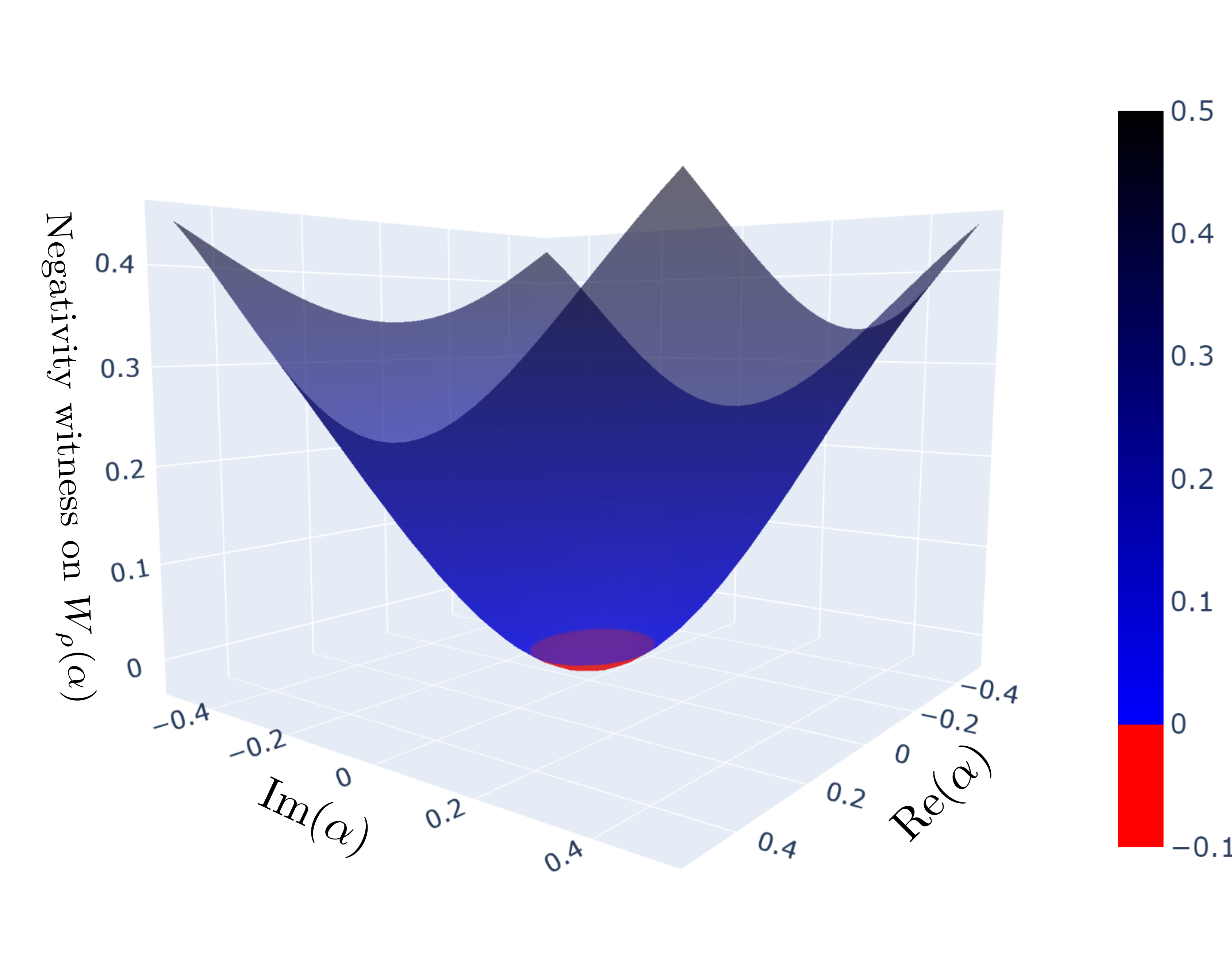
Figure 5: Negativity witnesses for a photon-subtracted squeezed vacuum state with $3$dB of squeezing and $0.95$ preparation purity. Using simulated samples from double homodyne detection, the witnesses in Eq. (12) have been estimated for a thousand values of the displacement amplitude $\alpha$, which have been interpolated for clarity, with a fixed precision $\epsilon=0.1$ and a fixed number of samples $N=5.5\times 10^{5}$. The curve has been shifted upwards by the value of $\epsilon$, and the red points witness the negativity of the state with at least $98\%$ confidence.

Note that the Wigner negativity witness corresponding to $n=1$ and $\alpha=0$ is simply the fidelity with the single-photon Fock state $\ket{1}$. If this fidelity is greater than $\frac{1}{2}$, then the Wigner function is negative at $\alpha=0$ (see Fig. 4, (b) and (c)). Using the expectation value estimation from section II.2 with the target operator $\hat{A}_{1}=\ket{1}\!\bra{1}$, we have simulated double homodyne sampling of an imperfect photon-subtracted squeezed vacuum state (see Fig. 5), and estimated the corresponding expectation values using the samples translated by $\alpha$, for several values of $\alpha=\alpha_{x}+i\alpha_{y}\in\mathbb{C}$, thus obtaining witnesses of its Wigner negativity.

V Discussion

Double homodyne detection is an operational measurement scheme that allows information on CV quantum states to be retrieved and quantum characteristics to be reliably probed. In this work, we obtained new results on the robustness of the stellar hierarchy of non-Gaussian quantum states and in particular on how to compute this robustness for a given target state with a simple optimisation. This allows us to make quantitative and robust statements about non-Gaussian states by deriving a class of witnesses based on the fidelity with specific non-Gaussian target states. Beyond the stellar rank and its operational characterization, we have also obtained new flexible Wigner negativity witnesses, which can be efficiently estimated from experimental data with analytical confidence intervals.

Our work shows that experimental demonstration of the newly introduced witnesses for stellar rank and Wigner negativity is feasible. The avenue towards such an experiment is by itself a direction of future research, since a detailed analysis of a wide range of experimental constraints is still required. Note, for example, that a dedicated analysis on the influence of imperfect double homodyne detection is an important next step.

On the level of theoretical work, a clear line of further research is to obtain robustness profiles of a wider variety of states, such as GKP states or cat states. These profiles will give a direct quantitative understanding of the difficulty of designing such states, as measured by the required number of photon additions and/or subtractions.

The certification technique on which this work is based has recently been extended to the multimode case Chabaud et al. (2020b), allowing the efficient computation of tight fidelity witnesses for a large class of multimode CV states. In combination with the use of entanglement witnesses, we expect that our methods will provide a reliable means of probing the interaction between entanglement and non-gaussianity. These techniques can thus be expected to contribute to the development of an experimental tool for detecting purely non-Gaussian entanglement Walschaers et al. (2017a). We leave this fascinating perspective for future work.

VI Acknowledgements

D.M. and F.G. acknowledge funding from the ANR through the ANR-17-CE24-0035 VanQuTe project. V.P. acknowledges financial support from the European Research Council under the Consolidator Grant COQCOoN (Grant No. 820079).

Appendix A Double homodyne expectation value estimation protocol

In this section, we first recall the double homodyne expectation value estimation protocol of Chabaud et al. (2019, 2020b) for a target operator $\hat{A}$ with bounded support over the Fock basis (section A.1). This protocol features several free parameters, which we then optimise in the case where the target operator is the density matrix of a Fock state: $\hat{A}=\ket{n}\!\bra{n}$, for $n\in\mathbb{N}$ (section A.2).

A.1 General protocol

Following Chabaud et al. (2019, 2020b), let us introduce for $k,l\geq 0$ the polynomials

$$\mathcal{L}_{k,l}(z) =e^{zz^{*}}\frac{(-1)^{k+l}}{\sqrt{k!}\sqrt{l!}}\frac{\partial^{k+l}}{\partial z^{k}\partial z^{*l}}e^{-zz^{*}}$$ (15)

$$=\sum_{p=0}^{\min{(k,l)}}{\frac{\sqrt{k!}\sqrt{l!}(-1)^{p}}{p!(k-p)!(l-p)!}z^{l-p}z^{*k-p}},$$

for $z\in\mathbb{C}$, which are, up to a normalisation, the Laguerre 2D polynomials. For all $k,l\in\mathbb{N}$, we define with these polynomials the functions

$$f_{k,l}(z,\eta):=\frac{1}{\eta^{1+\frac{k+l}{2}}}e^{\left(1-\frac{1}{\eta}\right)zz^{*}}\mathcal{L}_{l,k}\left(\frac{z}{\sqrt{\eta}}\right),$$ (16)

for all $z\in\mathbb{C}$ and all $0<\eta<1$. For all $k,l\in\mathbb{N}$, the function $z\mapsto f_{k,l}(z,\eta)$, being a polynomial multiplied by a converging Gaussian function, is bounded over $\mathbb{C}$. Let us define, for all $p\in\mathbb{N}^{*}$, all $z\in\mathbb{C}$ and all $0<\eta<1$,

$$g_{k,l}^{(p)}(z,\eta):=\sum_{j=0}^{p-1}{(-1)^{j}f_{k+j,l+j}(z,\eta)\,\eta^{j}\sqrt{\binom{k+j}{k}\binom{l+j}{l}}}.$$ (17)

and let

$$g_{\hat{A}}^{(p)}(z,\eta):=\sum_{k,l}{A_{kl}\,g_{k,l}^{(p)}(z,\eta)},$$ (18)

for any operator $\hat{A}=\sum_{k,l}{A_{kl}\ket{k}\!\bra{l}}$ with bounded support over the Fock basis. Let $N\in\mathbb{N}$, for all $\alpha_{1},\dots,\alpha_{N}\in\mathbb{C}$, we also define

$$F_{\hat{A}}(\alpha_{1},\dots,\alpha_{N})=\frac{1}{N}\sum_{i=1}^{N}{g_{\hat{A}}^{(p)}(\alpha_{i},\eta)},$$ (19)

thus omitting the dependencies in the free parameters $\eta$ and $p$. From Chabaud et al. (2020b) we have the following result:

Theorem.

Let $N\in\mathbb{N}^{*}$, let $\rho$ be a single-mode state and let $\alpha_{1},\dots,\alpha_{N}\in\mathbb{C}$ be samples of double homodyne detection of $N$ copies of $\rho$. Let $\epsilon>0$ and $\delta>0$. Then,

$$\left|\,\mathrm{Tr}(\hat{A}\rho)-F_{\hat{A}}(\alpha_{1},\dots,\alpha_{N})\right|\leq\epsilon$$ (20)

with probability greater than $1-\delta$, for a number of samples

$$N=\mathcal{O}\left(\frac{1}{\epsilon^{2+t}}\log\left(\frac{1}{\delta}\right)\right),$$ (21)

where $t>0$ is a free parameter depending on the choice of $\eta$ and $p$.

The expressions appearing in the theorem are generic and may be refined depending on the expression of the operator $\hat{A}$. Moreover, the choice of the free parameters $\eta$ and $p$ can be optimised in order to minimise the number of samples $N$ needed to achieve a given confidence interval $\epsilon,\delta$. We consider such an optimisation in the following section, in the case where $\hat{A}=\ket{n}\!\bra{n}$ is the density operator of a photon number Fock state $\ket{n}$, for $n\in\mathbb{N}$.

A.2 Optimised protocol for target Fock states

In this section, we optimise the certification protocol from the previous section for the case of photon number Fock states.

Let $0<\epsilon<1$ and $n\in\mathbb{N}$. In this section, we optimise the single-mode fidelity estimation protocol for a target Fock state $\ket{n}$. For $0<\eta<1$ and $p\in\mathbb{N}^{*}$, let

$$p_{n}:=\min\left\{q\geq p,\text{ s.t. }\eta\leq\left(1-\frac{p-1}{q}\right)\left(1-\frac{n}{n+q+1}\right)\right\}.$$ (22)

We denote by $\underset{\alpha\leftarrow D}{\mathbb{E}}[f(\alpha)]$ the expected value of a function $f$ for samples drawn from a distribution $D$. By Lemma 4 of Chabaud et al. (2020b) (in particular Eq. (A17) with $q_{0}=p_{n}$ and $k=l=n$),

$$\left|\underset{\alpha\leftarrow Q_{\rho}}{\mathbb{E}}[g_{n,n}^{(p)}(\alpha,\eta)]-\rho_{nn}\right|\leq\eta^{p_{n}}\binom{p_{n}-1}{p-1}\binom{n+p_{n}}{n}.$$ (23)

for any state $\rho$, where $g_{n,n}^{(p)}$ is defined in Eq. (17), for $k=l=n$. Moreover, by Lemma 4 of Chabaud et al. (2020b) we have

$$\underset{\alpha\leftarrow Q_{\rho}}{\mathbb{E}}[g_{n,n}^{(p)}(\alpha,\eta)]=\rho_{nn}+(-1)^{p+1}\sum_{q=p}^{+\infty}{\rho_{n+q,n+q}\eta^{q}\binom{q-1}{p-1}\binom{n+q}{q}}.$$ (24)

In particular, for $p$ odd,

$$\underset{\alpha\leftarrow Q_{\rho}}{\mathbb{E}}[g_{n,n}^{(p)}(\alpha,\eta)]\geq\rho_{nn},$$ (25)

i.e., $g_{n,n}^{(p)}$ overestimates $\rho_{nn}$, while for $p$ even,

$$\underset{\alpha\leftarrow Q_{\rho}}{\mathbb{E}}[g_{n,n}^{(p)}(\alpha,\eta)]\leq\rho_{nn},$$ (26)

i.e., $g_{n,n}^{(p)}$ underestimates $\rho_{nn}$. Hence, setting

$$h_{n}^{(p)}(z,\eta):=g_{n,n}^{(p)}(z,\eta)+\frac{1}{2}(-1)^{p}\eta^{p_{n}}\binom{p_{n}-1}{p-1}\binom{n+p_{n}}{n},$$ (27)

for all $z\in\mathbb{C}$, we obtain with Eq. (23),

$$\left|\underset{\alpha\leftarrow Q_{\rho}}{\mathbb{E}}[h_{n}^{(p)}(\alpha,\eta)]-\rho_{nn}\right|\leq\frac{1}{2}\eta^{p_{n}}\binom{p_{n}-1}{p-1}\binom{n+p_{n}}{n}.$$ (28)

The functions $z\mapsto h_{n}^{(p)}(z,\eta)$ and $z\mapsto g_{n,n}^{(p)}(z,\eta)$ only differ by a constant and thus have the same range. Let $N\in\mathbb{N}^{*}$ and let $\alpha_{1},\dots,\alpha_{N}\in\mathbb{C}$ be i.i.d. samples from double homodyne detection of a state $\rho$. For $n\in\mathbb{N}$, let us write

$$F_{n}(\alpha_{1},\dots,\alpha_{N}):=\frac{1}{N}\sum_{i=1}^{N}{h_{n}^{(p)}(\alpha_{i},\eta)},$$ (29)

where $h_{n}^{(p)}$ is defined in Eq. (27). With Hoeffding inequality Hoeffding (1963), we obtain

$$\Pr\left[\left|F_{n}(\alpha_{1},\dots,\alpha_{N})-\underset{\alpha\leftarrow Q_{\rho}}{\mathbb{E}}[h_{n}^{(p)}(\alpha,\eta)]\right|\geq\lambda\right]\leq 2\exp\left[-\frac{2N\lambda^{2}\eta^{2n+2}}{\left(R_{n}^{(p)}\right)^{2}}\right],$$ (30)

for all $p\in\mathbb{N}^{*}$ and all $\eta<1$, where $R_{n}^{(p)}$ is the range of the function

$$z\mapsto\eta^{n+1}g_{n}^{(p)}(z,\eta)=e^{-(1-\eta)\frac{|z|^{2}}{\eta}}\sum_{j=0}^{p-1}{(-1)^{n+j}\text{L}_{n+j}\left(\frac{|z|^{2}}{\eta}\right)\binom{n+j}{n}},$$ (31)

which is bounded for $0<\eta<1$. Combining Eqs. (28) and (30) we obtain

$$\left|\rho_{nn}-F_{n}(\alpha_{1},\dots,\alpha_{N})\right|\leq\lambda+\frac{1}{2}\eta^{p_{n}}\binom{p_{n}-1}{p-1}\binom{n+p_{n}}{n},$$ (32)

with probability greater than $1-P^{iid}_{n}$, where

$$P^{iid}_{n}:=2\exp\left[-\frac{2N\lambda^{2}\eta^{2n+2}}{\left(R_{n}^{(p)}\right)^{2}}\right].$$ (33)

Setting

$$\lambda=\max\left\{\epsilon-\frac{1}{2}\eta^{p_{n}}\binom{p_{n}-1}{p-1}\binom{n+p_{n}}{n},0\right\},$$ (34)

we finally obtain

$$\left|\rho_{nn}-F_{n}(\alpha_{1},\dots,\alpha_{N})\right|\leq\epsilon$$ (35)

with probability $1-P^{iid}_{n}$, where

$$P^{iid}_{n}=2\exp\left[-\frac{2N\lambda^{2}\eta^{2n+2}}{\left(R_{n}^{(p)}\right)^{2}}\right],$$ (36)

where

$$\lambda=\max\left\{\epsilon-\frac{1}{2}\eta^{p_{n}}\binom{p_{n}-1}{p-1}\binom{n+p_{n}}{n},0\right\}$$ (37)

$$p_{n}=\min\left\{q\geq p,\text{ s.t. }\eta\leq\left(1-\frac{p-1}{q}\right)\left(1-\frac{n}{n+q+1}\right)\right\}$$

$$R_{n}^{(p)}=\max_{z}\left[\eta^{n+1}g_{n}^{(p)}(z,\eta)\right]-\min_{z}\left[\eta^{n+1}g_{n}^{(p)}(z,\eta)\right]$$

$$\eta^{n+1}g_{n}^{(p)}(z,\eta)=(-1)^{n}e^{-(1-\eta)\frac{|z|^{2}}{\eta}}\sum_{j=0}^{p-1}{\text{L}_{n+j}\left(\frac{|z|^{2}}{\eta}\right)\binom{n+j}{n}}$$

$$\text{L}_{n}(x)=\sum_{i=0}^{n}{\frac{(-1)^{i}}{i!}\binom{n}{i}x^{i}},$$

for all $z\in\mathbb{C}$, all $x\in\mathbb{R}$, all $n\in\mathbb{N}$, all $p\in\mathbb{N}^{*}$, all $0<\eta<1$ and all $0<\epsilon<1$.

At this point, all expressions are analytical, optimised for the case of a target Fock state. The protocol still has two free parameters $p\in\mathbb{N}^{*}$ and $0<\eta<1$, once $\epsilon$, $n$ and $N$ are fixed. The procedure for optimising the efficiency of the protocol then consists in minimising the failure probability over the choice of these parameters $p,\eta$: for a target Fock state $\ket{n}$ with $n\in\mathbb{N}$ and a precision parameter $0<\epsilon<1$, we compute for increasing values of $p\in\mathbb{N}^{*}$, starting from $p=1$, the minimum failure probability $P^{iid}_{n}$ in Eq. (36) by optimising over the value of $\eta$; then, we pick the value of $p$ which minimises $P^{iid}_{n}$.

For example, for 95% confidence, i.e., $P^{iid}_{n}\leq 0.05$, we obtain in Table 1, 2 and 3 the number of samples $N$ necessary for the fidelity estimate precisions $\epsilon=0.1$, $0.2$ and $0.3$, for the target Fock states $\ket{n=0}$, $\ket{n=1}$ and $\ket{n=2}$, together with the values of the free parameters $p$ and $\eta$ and the corresponding value of $p_{n}$ (which is needed in the definition of the estimate $h_{n}^{(p)}$).

$\quad n\quad$	$N$	$\quad p\quad$	$\quad\eta\quad$	$\quad p_{n}\quad$
$0$	$\;2.7\times 10^{4}\;$	$3$	$0.34$	$4$
$1$	$\;5.5\times 10^{6}\;$	$3$	$0.26$	$3$
$2$	$\;1.3\times 10^{9}\;$	$3$	$0.21$	$3$

Table 1: Optimised parameters for target Fock states $0$, $1$ and $2$, for precision $\epsilon=0.1$ with 95% confidence.

$\quad n\quad$	$N$	$\quad p\quad$	$\quad\eta\quad$	$\quad p_{n}\quad$
$0$	$\;3.6\times 10^{3}\;$	$2$	$0.35$	$2$
$1$	$\;5.8\times 10^{5}\;$	$2$	$0.26$	$2$
$2$	$\;1.0\times 10^{8}\;$	$3$	$0.25$	$4$

Table 2: Optimised parameters for target Fock states $0$, $1$ and $2$, for a precision $\epsilon=0.2$ with 95% confidence.

$\quad n\quad$	$N$	$\quad p\quad$	$\quad\eta\quad$	$\quad p_{n}\quad$
$0$	$\;9.1\times 10^{2}\;$	$1$	$0.30$	$1$
$1$	$\;1.2\times 10^{5}\;$	$2$	$0.31$	$2$
$2$	$\;1.6\times 10^{7}\;$	$2$	$0.24$	$2$

Table 3: Optimised parameters for target Fock states $0$, $1$ and $2$, for a precision $\epsilon=0.3$ with 95% confidence.

In order to optimise further the efficiency of the protocol, we may replace the use of the Hoeffding inequality by a direct application of the central limit theorem (CLT). Instead of looking at the range of the distribution $h_{n}$, one can derive the variance of the sampled distribution. Then, one deduces a gaussian confidence interval of the mean estimation, since the central limit theorem ensures that the distribution of the mean converges towards a gaussian distribution. The theorem is valid for distribution whose variance is finite, which is the case for physical states.

Similarly, we obtain Eq. (36) with probability greater than $1-P^{iid}_{n,CLT}$, where

$$P^{iid}_{n,\text{CLT}}=1-\mathrm{erf}\left(\lambda\sqrt{\frac{N}{2\sigma^{2}}}\right),$$ (38)

$\sigma^{2}$ is the variance of the sampled estimations, and erf is the error function.

Applying the central limit theorem comes at the cost that the obtained bounds are no longer analytical, since we replace the theoretical variance by its value estimated from the samples.

To emphasize the usefulness of the optimisation carried out in this section, we have represented in Fig. 6 the difference in efficiency between the non-optimised protocol and its optimised versions, with Hoeffding inequality or CLT, for a target Fock state $\ket{2}$.

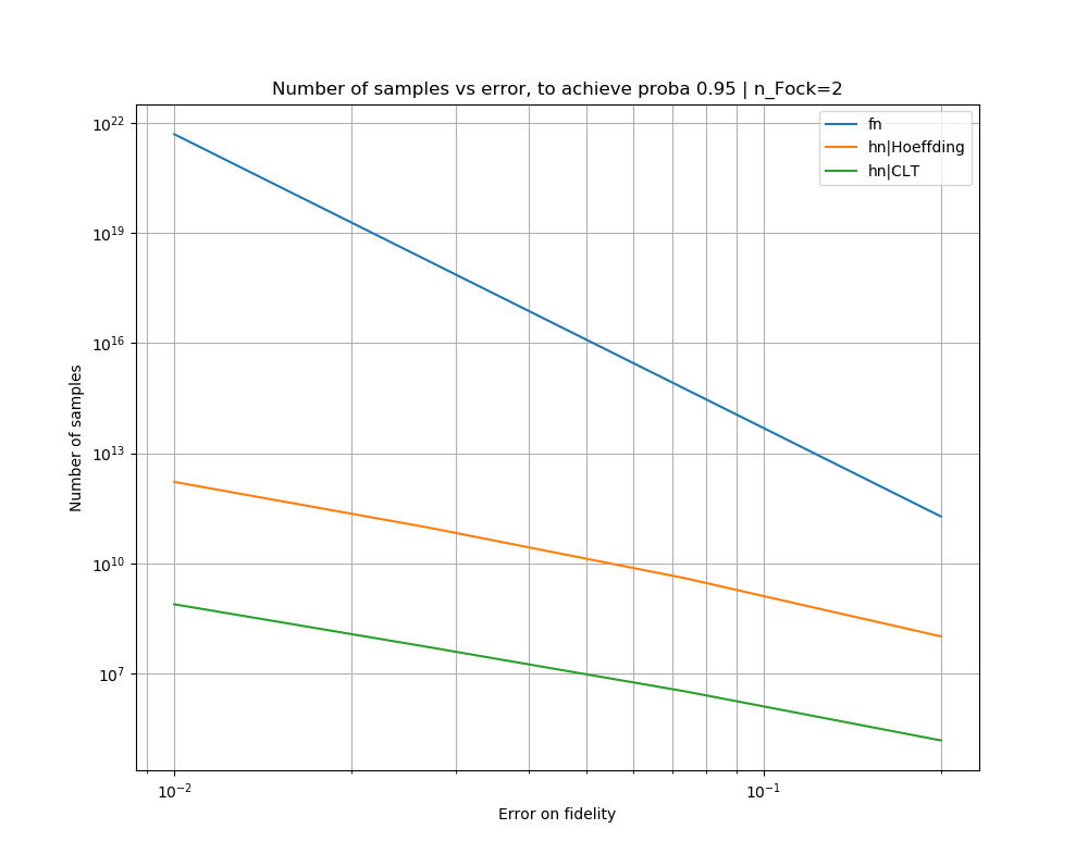
Figure 6: Efficiency of the various estimation methods for a target Fock state $\ket{2}$. The curves represent the number of samples necessary to obtain a given precision on the fidelity estimate with 95% confidence. The top curve is obtained using the protocol from Chabaud et al. (2019), the middle one using the optimised protocol with analytical bounds, and the bottom one using the improved bounds from the CLT (for which a Fock state $\ket{2}$ is sampled).

Appendix B Photon subtraction and stellar rank

The stellar function of a single-mode pure state $\ket{\psi}$ is defined as Chabaud et al. (2020a):

$$F_{\psi}^{\star}(z)=e^{\frac{1}{2}|z|^{2}}\braket{\psi}{z},$$ (39)

where $\ket{z}=e^{-\frac{1}{2}|z|^{2}}\sum{n\geq 0}{\frac{z^{n}}{\sqrt{n!}}\ket{n}}$ is the coherent state of amplitude $z$, for all $z\in\mathbb{C}$. This function gives a representation of a quantum state with a holomorphic function which is related to the Husimi $Q$ function by

$$Q_{\psi}(z)=\frac{e^{-|z|^{2}}}{\pi}\left|F_{\psi}^{\star}(z)\right|^{2}.$$ (40)

The stellar rank of a state $\ket{\psi}$ is the number of zeros of its stellar function (counted with multiplicity) and corresponds to the minimal number of elementary non-Gaussian operations—namely, photon-addition— necessary to engineer the state from the vacuum, together with unitary Gaussian operations.

While operators have their own treatment in the stellar formalism, it is sufficient for our purpose to consider the following correspondences: the creation and annihilation operators have the stellar representations Chabaud et al. (2020a)

$$\hat{a}^{\dagger}\rightarrow z,\quad\hat{a}\rightarrow\partial_{z},$$ (41)

i.e., the operator corresponding to $\hat{a}^{\dagger}$ in the stellar representation is the multiplication by $z$ and the operator in the stellar representation corresponding to $\hat{a}$ is the derivative with respect to $z$. This means that the stellar function of a photon-added state $\hat{a}^{\dagger}\ket{\psi}$ is given by $z\mapsto zF_{\psi}^{\star}(z)$, while the stellar function of a photon-subtracted state $\hat{a}\ket{\psi}$ is given by $z\mapsto\partial_{z}F_{\psi}^{\star}(z)$. In particular, photon-added states are always non-Gaussian Walschaers et al. (2017b), since $0$ is a root of their stellar function, while photon-subtracted states can be Gaussian (e.g., the Fock state $\ket{1}$, for which $\hat{a}\ket{1}=\ket{0}$, or the coherent states $\ket{\alpha}$, for $\alpha\in\mathbb{C}$, for which $\hat{a}\ket{\alpha}=\alpha\ket{\alpha}$).

Moreover, by Theorem 1 of Chabaud et al. (2020a), the stellar function of a state of finite stellar rank is a polynomial multiplied by a Gaussian function $\exp(Sz^{2}+Dz)$, where $S$ is a squeezing parameter and $D$ a displacement parameter. Hence, derivating this function gives another polynomial multiplied by the same Gaussian term. The new polynomial has a degree increased by $1$ if $S\neq 0$, the same degree if $S=0$ and $D\neq 0$, and a degree decreased by one if $S=D=0$. Hence, a single-photon subtraction can increase the stellar rank by at most $1$ since the number of zeros of the stellar functions is equal to the degree of this polynomial.

For completeness, note that the photon subtraction may conserve an infinite stellar rank (e.g., for a cat state) but may also make it finite (e.g., for a displaced cat state $\propto\ket{0}+\ket{\alpha}$).

Appendix C Proof of Lemma 7

For any pure state $\ket{\psi}\in\mathcal{H}_{\infty}$ and any set of pure states $\mathcal{X}$, we have

$$\sup_{\begin{subarray}{c}\rho=\sum{p_{i}{\ket{\phi}_{i}}\bra{\phi_{i}}}\\ \sum{p_{i}}=1,\phi_{i}\in\mathcal{X}\end{subarray}}{F(\rho,\psi)} =\sup_{\begin{subarray}{c}\rho=\sum{p_{i}{\ket{\phi}_{i}}\bra{\phi_{i}}}\\ \sum{p_{i}}=1,\phi_{i}\in\mathcal{X}\end{subarray}}{\braket{\psi}{\rho}{\psi}}$$ (42)

$$=\sup_{\sum{p_{i}}=1}\sup_{\phi_{i}\in\mathcal{X}}{\sum{p_{i}|\braket{\phi_{i}}{\psi}|^{2}}}$$

$$=\sup_{\phi\in\mathcal{X}}{|\braket{\phi}{\psi}|^{2}}$$

$$=\sup_{\phi\in\mathcal{X}}{F(\phi,\psi)}.$$

Hence, for $\mathcal{X}$ the set of pure states of stellar rank less than $k$,

$$R_{k}^{\star}(\psi) =\inf_{r^{\star}(\phi)<k}{D(\phi,\psi)}$$ (43)

$$=\inf_{r^{\star}(\phi)<k}{\sqrt{1-|\braket{\phi}{\psi}|^{2}}}$$

$$=\sqrt{1-\sup_{r^{\star}(\phi)<k}{F(\phi,\psi)}}$$

$$=\sqrt{1-\sup_{r^{\star}(\rho)<k}{F(\rho,\psi)}},$$

where $D$ denotes the trace distance, where we used the definition of the stellar rank for mixed states (3). We finally obtain

$$\sup_{r^{\star}(\rho)<k}{F(\rho,\psi)}=1-[R_{k}^{\star}(\psi)]^{2}.$$ (44)

∎

Appendix D Proof of Theorem 1

By Eq. (42) we have

$$\sup_{r^{\star}(\rho)<k}F(\rho,\psi)=\sup_{r^{\star}(\phi)<k}{|\braket{\phi}{\psi}|^{2}}.$$ (45)

By Theorem 4 of Chabaud et al. (2020a), for any pure state $\ket{\phi}$ such that $r^{\star}(\phi)<k$, there exist a normalised core state with a finite support over the Fock basis $\ket{C_{\phi}}$ of stellar rank lower than $k$ and a Gaussian operation $\hat{G}_{\phi}$ such that

$$\ket{\phi}=\hat{G}_{\phi}\ket{C_{\phi}}.$$ (46)

We obtain

$$|\braket{\phi}{\psi}|^{2} =|\braket{C_{\phi}}{\hat{G}_{\phi}^{\dagger}}{\psi}|^{2}$$ (47)

$$=|\braket{C_{\phi}}{\Pi_{k-1}\hat{G}_{\phi}^{\dagger}}{\psi}|^{2}$$

$$\leq|\braket{C_{\phi}}{C_{\phi}}|^{2}|\braket{\psi}{\hat{G}_{\phi}\Pi_{k-1}\hat{G}_{\phi}^{\dagger}}{\psi}|^{2}$$

$$=\,\mathrm{Tr}\left[\Pi_{k-1}\hat{G}_{\phi}^{\dagger}\ket{\psi}\bra{\psi}\hat{G}_{\phi}\right],$$

where we used $\ket{C_{\phi}}=\Pi_{k-1}\ket{C_{\phi}}$ in the second line, since $\ket{C_{\phi}}$ is a core state of stellar rank lower than $k$ (hence its support is contained in the support of $\Pi_{k-1}$), Cauchy-Schwarz inequality in the third line and $|\braket{C_{\phi}}{C_{\phi}}|^{2}=1$ in the last line. This upperbound is attained if

$$\ket{C_{\phi}}=\frac{\Pi_{k-1}\hat{G}_{\phi}^{\dagger}\ket{\psi}}{\sqrt{\,\mathrm{Tr}\left[\Pi_{k-1}\hat{G}_{\phi}^{\dagger}\ket{\psi}\bra{\psi}\hat{G}_{\phi}\right]}},$$ (48)

which is indeed a normalised core state of stellar rank lower than $k$.

With Eqs. (45) and (47), the maximum achievable fidelity with the state $\ket{\psi}$ is then given by

$$\sup_{r^{\star}(\rho)<k}F(\rho,\psi) =\sup_{\hat{G}_{\phi}\in\mathcal{G}}{\,\mathrm{Tr}\left[\Pi_{k-1}\hat{G}_{\phi}^{\dagger}\ket{\psi}\bra{\psi}\hat{G}_{\phi}\right]}$$ (49)

$$=\sup_{\hat{G}\in\mathcal{G}}{\,\mathrm{Tr}\left[\Pi_{k-1}\hat{G}\ket{\psi}\bra{\psi}\hat{G}^{\dagger}\right]},$$

where the supremum is over Gaussian unitary operations and where we used the fact that the set of Gaussian unitary operations is invariant under adjoint in the second line. With Eq. (46), assuming the optimisation yields an optimal Gaussian unitary $\hat{G}_{0}$, an optimal approximating state is $\ket{\phi}=\hat{G}_{\phi}\ket{C_{\phi}}$, where $\hat{G}_{\phi}=\hat{G}_{0}^{\dagger}$ and where $\ket{C_{\phi}}$ is given by Eq. (48). Namely,

$$\ket{\phi}=\hat{G}_{0}^{\dagger}\left(\frac{\Pi_{k-1}\hat{G}_{0}\ket{\psi}}{\left\|\Pi_{k-1}\hat{G}_{0}\ket{\psi}\right\|}\right),$$ (50)

i.e., $\hat{G}_{0}\ket{\phi}$ is the renormalised truncation of $\hat{G}_{0}\ket{\psi}$ at photon number $k-1$.

∎

Appendix E Certifying the stellar rank

E.1 Achievable fidelities with states of stellar rank 1

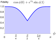
Figure 7: Achievable fidelities with target core states $\cos\phi\ket{0}+e^{i\chi}\sin\phi\ket{1}$ using Gaussian states, for all $\phi,\chi\in[0,2\pi]$, as a function of $\phi$.

We have computed numerically the maximum achievable fidelities between Gaussian states and states of the form

$$\cos\phi\ket{0}+e^{i\chi}\sin\phi\ket{1}.$$ (51)

These are independent of $\chi$ and are depicted in Fig. 7 as a function of $\phi$.

The most robust state of stellar rank $1$ is the Fock state $\ket{1}$ (and all the states that are obtained from it with Gaussian unitary operations), corresponding to $\phi=\frac{\pi}{2}$, as it features the minimal achievable fidelity with Gaussian states.

E.2 Achievable fidelities with Fock states

In this section, we prove the following result:

Lemma 1.

Let $k\in\mathbb{N}^{*}$ and let $n\in\mathbb{N}$. Then, the maximum achievable fidelity with the Fock state $\ket{n}$ using states of stellar rank less than $k$ is given by

$$\sup_{r^{\star}(\rho)<k}\braket{n}{\rho}{n}=\sup_{\xi,\alpha\in\mathbb{C}}{\sum_{m=0}^{k-1}{|u_{m,n}(\xi,\alpha)|^{2}}},$$ (52)

where for all $m\in\{0,\dots,k-1\}$ and all $\xi=re^{i\theta},\alpha\in\mathbb{C}$,

$$u_{m,n}(\xi,\alpha)=\frac{1}{\sqrt{m!n!c_{r}}}\left[\partial_{z}^{n}(c_{r}z+s_{r}e^{i\theta}\partial_{z}-\alpha^{*})^{m}e^{-\frac{1}{2}e^{-i\theta}t_{r}z^{2}+\frac{\alpha}{c_{r}}z+\frac{1}{2}e^{i\theta}t_{r}\alpha^{2}-\frac{1}{2}|\alpha|^{2}}\right]_{z=0},$$ (53)

with $c_{r}=\cosh r$, $s_{r}=\sinh r$ and $t_{r}=\tanh r$. Moreover, assuming the optimisation yields values $\xi_{0},\alpha_{0}\in\mathbb{C}$, an optimal approximating state is

$$\hat{D}^{\dagger}(\alpha_{0})\hat{S}^{\dagger}(\xi_{0})\left(\frac{\Pi_{k-1}\hat{S}(\xi_{0})\hat{D}(\alpha_{0})\ket{n}}{\left\|\Pi_{k-1}\hat{S}(\xi_{0})\hat{D}(\alpha_{0})\ket{n}\right\|}\right).$$ (54)

Proof.

From Theorem 1 we have

$$\sup_{r^{\star}(\rho)<k}F(\rho,n) =\sup_{r^{\star}(\rho)<k}\braket{n}{\rho}{n}$$ (55)

$$=\sup_{\hat{G}\in\mathcal{G}}{\,\mathrm{Tr}\left[\Pi_{k-1}\hat{G}\ket{n}\bra{n}\hat{G}^{\dagger}\right]}$$

$$=\sup_{\xi,\alpha\in\mathbb{C}}{\,\mathrm{Tr}\left[\Pi_{k-1}\hat{D}^{\dagger}(\alpha)\hat{S}^{\dagger}(\xi)\ket{n}\bra{n}\hat{S}(\xi)\hat{D}(\alpha)\right]}$$

$$=\sup_{\xi,\alpha\in\mathbb{C}}{\sum_{m=0}^{k-1}\left|\braket{n}{\hat{S}(\xi)\hat{D}(\alpha)}{m}\right|^{2}},$$

where we used the fact that any single-mode Gaussian unitary operation may be decomposed as a squeezing and a displacement. Assuming the optimisation yields values $\xi_{0},\alpha_{0}\in\mathbb{C}$, the optimal core state used in the approximation is

$$\ket{C}=\frac{\Pi_{k-1}\hat{S}(\xi_{0})\hat{D}(\alpha_{0})\ket{n}}{\left\|\Pi_{k-1}\hat{S}(\xi_{0})\hat{D}(\alpha_{0})\ket{n}\right\|}.$$ (56)

Now for all $m\in\{0,\dots,k-1\}$,

$$\braket{n}{\hat{S}(\xi)\hat{D}(\alpha)}{m} =\frac{1}{\sqrt{m!n!}}\braket{0}{\hat{a}^{n}\hat{S}(\xi)\hat{D}(\alpha)(\hat{a}^{\dagger})^{m}}{0}$$ (57)

$$=\frac{1}{\sqrt{m!n!}}\braket{0}{\hat{a}^{n}(c_{r}\hat{a}^{\dagger}+s_{r}e^{i\theta}\hat{a}-\alpha^{*})^{m}\hat{S}(\xi)\hat{D}(\alpha)}{0},$$

with $c_{r}=\cosh r$, $s_{r}=\sinh r$. Hereafter we also set $t_{r}=\tanh r$. We have $\braket{0}{\chi}=F^{\star}_{\chi}(0)$ for all states $\chi$, hence switching to the stellar representation Chabaud et al. (2020a) we obtain

$$\braket{n}{\hat{S}(\xi)\hat{D}(\alpha)}{m}=\frac{1}{\sqrt{m!n!c_{r}}}\left[\partial_{z}^{n}\left(c_{r}z+s_{r}e^{i\theta}\partial_{z}-\alpha^{*}\right)^{m}e^{-\frac{1}{2}e^{-i\theta}t_{r}z^{2}+\frac{\alpha}{c_{r}}z+\frac{1}{2}e^{i\theta}t_{r}\alpha^{2}-\frac{1}{2}|\alpha|^{2}}\right]_{z=0}.$$ (58)

Setting, for all $m\in\{0,\dots,k-1\}$, $u_{m,n}(\xi,\alpha)=\braket{n}{\hat{S}(\xi)\hat{D}(\alpha)}{m}$, we finally obtain with Eq. (55),

$$\sup_{r^{\star}(\rho)<k}\braket{n}{\rho}{n}=\sup_{\xi,\alpha\in\mathbb{C}}{\sum_{m=0}^{k-1}{|u_{m,n}(\xi,\alpha)|^{2}}},$$ (59)

where for all $m\in\{0,\dots,k-1\}$ and all $\xi=re^{i\theta},\alpha\in\mathbb{C}$,

$$u_{m}(\xi,\alpha)=\frac{1}{\sqrt{m!n!c_{r}}}\left[\partial_{z}^{n}(c_{r}z+s_{r}e^{i\theta}\partial_{z}-\alpha^{*})^{m}e^{-\frac{1}{2}e^{-i\theta}t_{r}z^{2}+\frac{\alpha}{c_{r}}z+\frac{1}{2}e^{i\theta}t_{r}\alpha^{2}-\frac{1}{2}|\alpha|^{2}}\right]_{z=0},$$ (60)

with $c_{r}=\cosh r$, $s_{r}=\sinh r$ and $t_{r}=\tanh r$. Moreover, assuming the optimisation yields values $\xi_{0},\alpha_{0}\in\mathbb{C}$, an optimal approximating state is $\ket{\phi}=\hat{D}^{\dagger}(\alpha_{0})\hat{S}^{\dagger}(\xi_{0})\ket{C}$, where $\ket{C}$ is defined in Eq. (56). Namely,

$$\ket{\phi}=\hat{D}^{\dagger}(\alpha_{0})\hat{S}^{\dagger}(\xi_{0})\left(\frac{\Pi_{k-1}\hat{S}(\xi_{0})\hat{D}(\alpha_{0})\ket{n}}{\left\|\Pi_{k-1}\hat{S}(\xi_{0})\hat{D}(\alpha_{0})\ket{n}\right\|}\right),$$ (61)

i.e., $\hat{S}(\xi_{0})\hat{D}(\alpha_{0})\ket{\phi}$ is the renormalised truncation of $\hat{S}(\xi_{0})\hat{D}(\alpha_{0})\ket{C_{\psi}}$ at photon number $k-1$.

∎

From this expression we have obtained numerically the maximum achievable fidelities up to $n=5$. The table below summarises the results, with the convention $r=k+1$.

	0	1	2	3	4	5
0	1	1	1	1	1	1
1	0.478	1	1	1	1	1
2	0.381	0.557	1	1	1	1
3	0.333	0.462	0.593	1	1	1
4	0.301	0.409	0.501	0.612	1	1
5	0.279	0.374	0.449	0.525	0.626	1

Table 4: Maximum achievable fidelities with Fock states $\ket{n}$ using states with stellar rank less or equal to $r$, for $n,r\in\{0,\dots,5\}$.

References

- Monz et al. (2016) T. Monz, D. Nigg, E. A. Martinez, M. F. Brandl, P. Schindler, R. Rines, S. X. Wang, I. L. Chuang, and R. Blatt, Realization of a scalable shor algorithm, Science 351, 1068 (2016).
- Wang et al. (2019) H. Wang, J. Qin, X. Ding, M.-C. Chen, S. Chen, X. You, Y.-M. He, X. Jiang, L. You, Z. Wang, C. Schneider, J. J. Renema, S. Höfling, C.-Y. Lu, and J.-W. Pan, Boson sampling with 20 input photons and a 60-mode interferometer in a -dimensional hilbert space, Phys. Rev. Lett. 123, 250503 (2019).
- Arute et al. (2019) F. Arute, K. Arya, R. Babbush, D. Bacon, J. C. Bardin, R. Barends, R. Biswas, S. Boixo, F. G. S. L. Brandao, D. A. Buell, B. Burkett, Y. Chen, Z. Chen, B. Chiaro, R. Collins, W. Courtney, A. Dunsworth, E. Farhi, B. Foxen, A. Fowler, C. Gidney, M. Giustina, R. Graff, K. Guerin, S. Habegger, M. P. Harrigan, M. J. Hartmann, A. Ho, M. Hoffmann, T. Huang, T. S. Humble, S. V. Isakov, E. Jeffrey, Z. Jiang, D. Kafri, K. Kechedzhi, J. Kelly, P. V. Klimov, S. Knysh, A. Korotkov, F. Kostritsa, D. Landhuis, M. Lindmark, E. Lucero, D. Lyakh, S. Mandrà, J. R. McClean, M. McEwen, A. Megrant, X. Mi, K. Michielsen, M. Mohseni, J. Mutus, O. Naaman, M. Neeley, C. Neill, M. Y. Niu, E. Ostby, A. Petukhov, J. C. Platt, C. Quintana, E. G. Rieffel, P. Roushan, N. C. Rubin, D. Sank, K. J. Satzinger, V. Smelyanskiy, K. J. Sung, M. D. Trevithick, A. Vainsencher, B. Villalonga, T. White, Z. J. Yao, P. Yeh, A. Zalcman, H. Neven, and J. M. Martinis, Quantum supremacy using a programmable superconducting processor, Nature 574, 505 (2019).
- Jurcevic et al. (2020) P. Jurcevic, A. Javadi-Abhari, L. S. Bishop, I. Lauer, D. F. Bogorin, M. Brink, L. Capelluto, O. Günlük, T. Itoko, N. Kanazawa, A. Kandala, G. A. Keefe, K. Krsulich, W. Landers, E. P. Lewandowski, D. T. McClure, G. Nannicini, A. Narasgond, H. M. Nayfeh, E. Pritchett, M. B. Rothwell, S. Srinivasan, N. Sundaresan, C. Wang, K. X. Wei, C. J. Wood, J.-B. Yau, E. J. Zhang, O. E. Dial, J. M. Chow, and J. M. Gambetta, Demonstration of quantum volume 64 on a superconducting quantum computing system (2020), arXiv:2008.08571 [quant-ph] .
- Braunstein and van Loock (2005) S. L. Braunstein and P. van Loock, Quantum information with continuous variables, Rev. Mod. Phys. 77, 513 (2005).
- Pfister (2019) O. Pfister, Continuous-variable quantum computing in the quantum optical frequency comb, Journal of Physics B: Atomic, Molecular and Optical Physics 53, 012001 (2019).
- Bourassa et al. (2020) J. E. Bourassa, R. N. Alexander, M. Vasmer, A. Patil, I. Tzitrin, T. Matsuura, D. Su, B. Q. Baragiola, S. Guha, G. Dauphinais, K. K. Sabapathy, N. C. Menicucci, and I. Dhand, Blueprint for a scalable photonic fault-tolerant quantum computer (2020), arXiv:2010.02905 [quant-ph] .
- Larsen et al. (2019) M. V. Larsen, X. Guo, C. R. Breum, J. S. Neergaard-Nielsen, and U. L. Andersen, Deterministic generation of a two-dimensional cluster state, Science 366, 369 (2019).
- Asavanant et al. (2019) W. Asavanant, Y. Shiozawa, S. Yokoyama, B. Charoensombutamon, H. Emura, R. N. Alexander, S. Takeda, J.-i. Yoshikawa, N. C. Menicucci, H. Yonezawa, and A. Furusawa, Generation of time-domain-multiplexed two-dimensional cluster state, Science 366, 373 (2019).
- Campagne-Ibarcq et al. (2020) P. Campagne-Ibarcq, A. Eickbusch, S. Touzard, E. Zalys-Geller, N. E. Frattini, V. V. Sivak, P. Reinhold, S. Puri, S. Shankar, R. J. Schoelkopf, L. Frunzio, M. Mirrahimi, and M. H. Devoret, Quantum error correction of a qubit encoded in grid states of an oscillator, Nature 584, 368 (2020).
- Cahill and Glauber (1969) K. E. Cahill and R. J. Glauber, Density operators and quasiprobability distributions, Physical Review 177, 1882 (1969).
- Su et al. (2012) X. Su, Y. Zhao, S. Hao, X. Jia, C. Xie, and K. Peng, Experimental preparation of eight-partite cluster state for photonic qumodes, Opt. Lett. 37, 5178 (2012).
- Roslund et al. (2014) J. Roslund, R. Medeiros de Araújo, S. Jiang, C. Fabre, and N. Treps, Wavelength-multiplexed quantum networks with ultrafast frequency combs, Nature Photonics 8, 109 (2014).
- Chen et al. (2014) M. Chen, N. C. Menicucci, and O. Pfister, Experimental realization of multipartite entanglement of 60 modes of a quantum optical frequency comb, Phys. Rev. Lett. 112, 120505 (2014).
- Yoshikawa et al. (2016) J.-i. Yoshikawa, S. Yokoyama, T. Kaji, C. Sorphiphatphong, Y. Shiozawa, K. Makino, and A. Furusawa, Generation of one-million mode continuous-variable cluster state by unlimited time-domain multiplexing, arXiv:1606.06688 (2016).
- Weedbrook et al. (2012) C. Weedbrook, S. Pirandola, R. García-Patrón, N. J. Cerf, T. C. Ralph, J. H. Shapiro, and S. Lloyd, Gaussian quantum information, Rev. Mod. Phys. 84, 621 (2012).
- Bartlett et al. (2002) S. D. Bartlett, B. C. Sanders, S. L. Braunstein, and K. Nemoto, Efficient classical simulation of continuous variable quantum information processes, Phys. Rev. Lett. 88, 097904 (2002).
- Mari and Eisert (2012) A. Mari and J. Eisert, Positive wigner functions render classical simulation of quantum computation efficient, Phys. Rev. Lett. 109, 230503 (2012).
- Rahimi-Keshari et al. (2016) S. Rahimi-Keshari, T. C. Ralph, and C. M. Caves, Sufficient conditions for efficient classical simulation of quantum optics, Phys. Rev. X 6, 021039 (2016).
- Filip and Mišta Jr (2011) R. Filip and L. Mišta Jr, Detecting quantum states with a positive wigner function beyond mixtures of gaussian states, Physical Review Letters 106, 200401 (2011).
- Genoni et al. (2013) M. G. Genoni, M. L. Palma, T. Tufarelli, S. Olivares, M. Kim, and M. G. Paris, Detecting quantum non-gaussianity via the wigner function, Physical Review A 87, 062104 (2013).
- Chabaud et al. (2020a) U. Chabaud, D. Markham, and F. Grosshans, Stellar representation of non-gaussian quantum states, Physical Review Letters 124, 063605 (2020a).
- Lvovsky and Raymer (2009) A. I. Lvovsky and M. G. Raymer, Continuous-variable optical quantum-state tomography, Reviews of Modern Physics 81, 299 (2009).
- Tiunov et al. (2020) E. S. Tiunov, V. V. T. (Vyborova), A. E. Ulanov, A. I. Lvovsky, and A. K. Fedorov, Experimental quantum homodyne tomography via machine learning, Optica 7, 448 (2020).
- Eisert et al. (2019) J. Eisert, D. Hangleiter, N. Walk, I. Roth, D. Markham, R. Parekh, U. Chabaud, and E. Kashefi, Quantum certification and benchmarking, arXiv preprint arXiv:1910.06343 (2019).
- Silva et al. (2017) G. B. Silva, S. Glancy, and H. M. Vasconcelos, Investigating bias in maximum-likelihood quantum-state tomography, Phys. Rev. A 95, 022107 (2017).
- Blume-Kohout (2010) R. Blume-Kohout, Optimal, reliable estimation of quantum states, New Journal of Physics 12, 043034 (2010).
- Faist and Renner (2016) P. Faist and R. Renner, Practical and reliable error bars in quantum tomography, Phys. Rev. Lett. 117, 010404 (2016).
- Cimini et al. (2020) V. Cimini, M. Barbieri, N. Treps, M. Walschaers, and V. Parigi, Neural networks for detecting multimode wigner negativity, Phys. Rev. Lett. 125, 160504 (2020).
- Paris (1996a) M. G. Paris, Quantum state measurement by realistic heterodyne detection, Physical Review A 53, 2658 (1996a).
- Ferraro et al. (2005) A. Ferraro, S. Olivares, and M. G. Paris, Gaussian states in continuous variable quantum information, arXiv preprint quant-ph/0503237 (2005).
- Chabaud et al. (2019) U. Chabaud, T. Douce, F. Grosshans, E. Kashefi, and D. Markham, Building trust for continuous variable quantum states, arXiv preprint arXiv:1905.12700 (2019).
- Aaronson and Arkhipov (2013) S. Aaronson and A. Arkhipov, The computational complexity of linear optics, Theory of Computing 9, 143 (2013).
- Chabaud et al. (2020b) U. Chabaud, F. Grosshans, E. Kashefi, and D. Markham, Efficient verification of boson sampling, arXiv preprint arXiv:2006.03520 (2020b).
- Chabaud et al. (2017) U. Chabaud, T. Douce, D. Markham, P. Van Loock, E. Kashefi, and G. Ferrini, Continuous-variable sampling from photon-added or photon-subtracted squeezed states, Physical Review A 96, 062307 (2017).
- Menzies and Filip (2009) D. Menzies and R. Filip, Gaussian-optimized preparation of non-gaussian pure states, Physical Review A 79, 012313 (2009).
- Paris (1996b) M. G. Paris, On density matrix reconstruction from measured distributions, Optics communications 124, 277 (1996b).
- Lütkenhaus and Barnett (1995) N. Lütkenhaus and S. M. Barnett, Nonclassical effects in phase space, Physical Review A 51, 3340 (1995).
- Ra et al. (2020) Y.-S. Ra, A. Dufour, M. Walschaers, C. Jacquard, T. Michel, C. Fabre, and N. Treps, Non-gaussian quantum states of a multimode light field, Nature Physics 16, 144 (2020).
- Royer (1977) A. Royer, Wigner function as the expectation value of a parity operator, Physical Review A 15, 449 (1977).
- Fiurášek and Ježek (2013) J. Fiurášek and M. Ježek, Witnessing negativity of wigner function by estimating fidelities of catlike states from homodyne measurements, Physical Review A 87, 062115 (2013).
- Walschaers et al. (2017a) M. Walschaers, C. Fabre, V. Parigi, and N. Treps, Entanglement and wigner function negativity of multimode non-gaussian states, Phys. Rev. Lett. 119, 183601 (2017a).
- Hoeffding (1963) W. Hoeffding, Probability inequalities for sums of bounded random variables, Journal of the American statistical association 58, 13 (1963).
- Walschaers et al. (2017b) M. Walschaers, C. Fabre, V. Parigi, and N. Treps, Statistical signatures of multimode single-photon-added and-subtracted states of light, Physical Review A 96, 053835 (2017b).