A multi-layer reactive transport model for fractured porous media

Abstract

An accurate modeling of reactive flows in fractured porous media is a key ingredient to obtain reliable numerical simulations of several industrial and environmental applications. For some values of the physical parameters we can observe the formation of a narrow region or layer around the fractures where chemical reactions are focused. Here the transported solute may precipitate and form a salt, or vice-versa. This phenomenon has been observed and reported in real outcrops. By changing its physical properties this layer might substantially alter the global flow response of the system and thus the actual transport of solute: the problem is thus non-linear and fully coupled. The aim of this work is to propose a new mathematical model for reactive flow in fractured porous media, by approximating both the fracture and these surrounding layers via a reduced model. In particular, our main goal is to describe the layer thickness evolution with a new mathematical model, and compare it to a fully resolved equidimensional model for validation. As concerns numerical approximation we extend an operator splitting scheme in time to solve sequentially, at each time step, each physical process thus avoiding the need for a non-linear monolithic solver, which might be challenging due to the non-smoothness of the reaction rate. We consider bi- and tridimensional numerical test cases to asses the accuracy and benefit of the proposed model in realistic scenarios.

1 Introduction

The study of reactive flows in porous media is a challenging problem in a large variety of applications, from geothermal energy to $CO_{2}$ sequestration up to the study of flow in tissues or that of the degradation of monuments and cultural heritage sites. In many cases the porous material presents networks of fractures that may greatly affect the flow field. These fractures could be responsible for the fast transport of reactants and heat and thus, in the proximity of fractures, it is possible to observe strong geochemical effects such as mineral precipitation, dissolution of transformation that can significantly alter the structure of the porous matrix. Depending on the relative speed of reaction and transport, namely depending on Damköler number, we can observe different patterns: a diffused effect on a large part of the domain, or steeper concentration profiles leading to mineral precipitation focusing in thin layers around the fractures.

This work presents a mathematical model for this phenomenon based on a geometrical model reduction that allows to represent thin, heterogeneous portions of the domains, such as fractures, as lower dimensional manifolds immersed in the rock matrix. The proposed model does indeed follow an important line of research of flow in fractured porous media where fractures are modeled as one-codimensional manifolds (typically planar) immersed in porous media. These models, often indicated as hybrid, or mixed-dimensional, describe the evolution of flow and related fields inside the fracture using a dimensionally reduced set of equations, and coupling conditions with the surrounding porous media. With no pretence of being exhaustive, we give a brief overview of literature related to the techniques used in this framework. A first hybrid-dimensional model for the coupling of Darcy’s flow in porous media and a single immersed fracture has been presented in [32], and later extended to networks of fractures by several authors, among which [19, 38, 22]. In all those works single-phase flow was considered, while in [24, 12, 1] the authors deal with two-phase flow formulation. To treat this class of problems, a large variety of numerical schemes have been exploited. The literature on the subject is vary vast, we give here only a few suggestions for the interested readers. Discretization methods for this type of problems are broadly subdivided into conforming and non-conforming. In a conforming method the computational grid used for the porous media is conformal to that used in the fractures, which means that the elements of the grid used to discretize the fractures coincide geometrically with facets of the mesh used for the porous medium. In this setting, many numerical schemes have been proposed, from classical finite volume approaches, like in [39], to mimetic finite differencing [5], gradient schemes [13], discontinuous Galerkin [4] and hybrid-high order schemes [15], just to mention some recent works. We recall also some literature concerning non-conforming methods, which can be again subdivided into two subsets. The first concerns the so called geometrically non-matching discretizations, where the grid used in the fracture is completely independent to that of the porous media. Among this type of techniques we mention the embedded discrete fracture network (e-DFM) [23, 40] and approaches based on the use of eXtended finite elements [18]. In the second set we have techniques where the fracture is still geometrically conforming with the porous media grid, but the computational grid can be different on the two sides. In this class we mention the framework presented in [9, 33] where a mortaring-type technique is used to connect the solution on domains of different dimensions. See also [17, 7] for a comparison of some of these models.

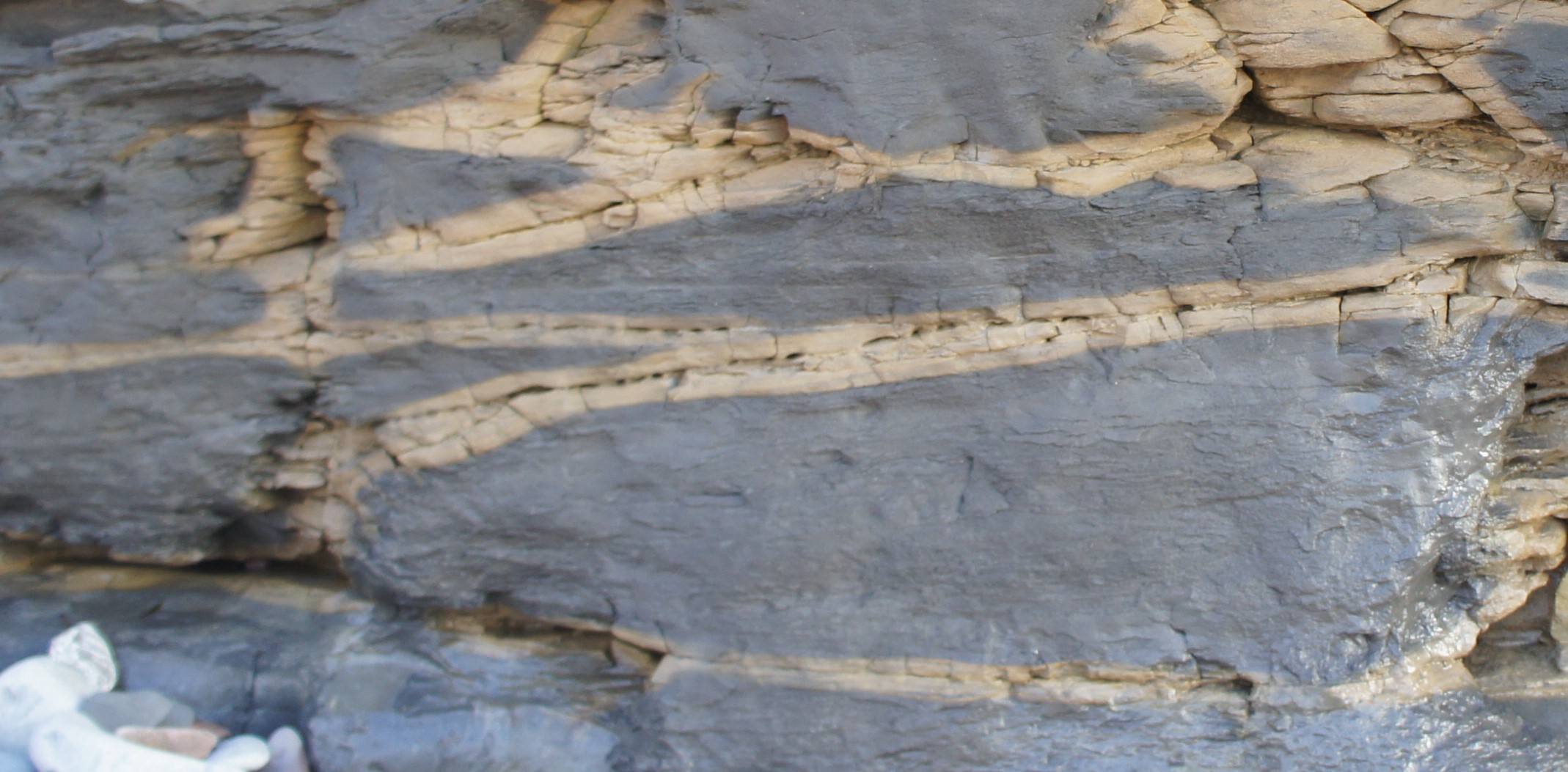
Figure 1: An example of fractures where it is evident the presence of a thin layer of altered material in the vicinity of the fracture. The alteration is due to geochemical processes driven by the fluid carried by the fractures.

In this paper we extend the model presented in [27, 25], where the authors developed a model for flow in fractured media accounting for dissolution-precipitation processes that may alter the flow behavior in of both fractures and rock matrix. In  [27, 25] the fracture is represented by an immersed one-codimensional manifold and special interface conditions were devised for the diffusion-transport-reaction problem. However, it is known, see Figure 1, that the geochemical processes may heavily affect a very thin layer around the fracture. Simulating the processes in that region is crucial, but since it is part of the rock matrix we would need a very fine grid resolution to obtain an accurate approximation. Consequently, in this work we consider a model where also those layers are described with a one-codimensional representation. Thus, the proposed hybrid-dimensional model comprises three embedded structures, one for the fracture and two for the damage zone surrounding the fracture at the two sides. We consider the simple reaction model for solute/mineral reactions illustrated in [25], in particular we will consider a single mobile species dissolved in water, representing one of the two ions in a salt precipitation reaction, and track its transport solving the single phase Darcy problem and a suitable advection-diffusion-reaction PDE. Simultaneously, we will keep track of the corresponding precipitate concentration in the domain. The model is similar to the one proposed in [16, 21, 25, 31, 26] to model fault cores and their surrounding damage zones. It couples three lower dimensional domains among them and with the surrounding porous matrix by means of multi-dimensional conservation operators and suitable interface conditions. This procedure is applied to the Darcy problem and to the evolution equation for the solute concentration. It could be easily extended to the heat equation to obtain a more complete physical description of the problem. Another original contributions of this work consists in the fact that the thickness of the reactive layers is not fixed a priori, but computed at each time based on the local Darcy velocity and solute concentration. To this aim, we have derived a simplified problem on the direction normal to the fracture that provides an idealized, but useful estimate of the area affected by precipitation.

The numerical discretization is based on a sequential operator splitting strategy for the decoupling of the equations, and on mixed finite elements for a good spatial approximation of the fluxes. The model is implemented in the open source library PorePy, a simulation tool for fractured and deformable porous media written in Python, see [29]. Some numerical tests are presented, with the aim of verifying the applicability of the proposed reduced model and its limits, for both two and three-dimensional settings.

The paper is structured as follows: in Section 2 the single and multi-layer mathematical model is introduced and described in details. We introduce also the model to describe the evolution of the layer surrounding the fracture. Section 3 defines the numerical discretization, in space and time. In particular, a splitting scheme in time is detailed to allow the solution of each physical process sequentially. In Section 4 we present the numerical test cases for the comparison between the new model and the one already present in literature. Finally, Section 5 is devoted to the conclusions.

2 Mathematical model

Let us start by illustrating the governing equations before performing dimensional reduction of the fracture region. We will consider here a simple setting with a single fracture, and depict the domains in two dimensions for simplicity, even if the presentation is given in a general setting and three-dimensional results will be presented in Section 4.

Let $\Theta\subset\mathbb{R}^{d}$, with $d=2$ or $3$, be the domain filled by porous material, where we can identify three parts, as depicted in Figure 2: the porous matrix $\Omega$, occupying the larger part of the domain; the fracture $\gamma$, characterized by a small thickness, called aperture, and a disconnected subdomain $\mu$, formed by two layers ($\mu^{-}$ and $\mu^{+}$) adjacent the fracture at both sides. The domain $\Omega$ is split in two disjoint parts $\Omega^{+}$ and $\Omega^{-}$ by the two sides of the layer. Clearly, $\overline{\Theta}=\overline{\Omega}\cup\overline{\gamma}\cup\overline{\mu}$ and $\Omega$, $\gamma$, and $\mu$ have mutually disjoint interior. In the following, barred quantities are given boundary data.

Figure 2: Equi-dimensional representation of the rock matrix $\Omega$, the fracture $\gamma$ and surrounding layers $\mu$.

We assume that $\Theta$ is filled by a single phase fluid, water, with constant density, and that average fluid velocity $\bm{q}_{\Theta}$ and pressure $p_{\Theta}$ can be obtained as the solution of the Darcy’s problem

$$\begin{aligned} &\begin{aligned} &k_{\Theta}^{-1}\bm{q}_{\Theta}+\nabla p_{\Theta}=\bm{0}\\ &\partial_{t}\phi_{\Theta}+\nabla\cdot\bm{q}_{\Theta}+f_{\Theta}=0\end{aligned}\quad&&\text{in }\Theta\times(0,T)\\ &p_{\Theta}=\overline{p_{\Theta}}&&\text{on }\partial\Theta_{p}\times(0,T)\\ &\bm{q}_{\Theta}\cdot\bm{\nu}=\overline{q_{\Theta}}&&\text{on }\partial\Theta_{q}\times(0,T)\end{aligned}$$ (1)

where $\phi_{\Theta}$ denotes the porosity (variable in space and time), $k_{\Theta}=k_{\Theta}(\phi_{\Theta})$ is the intrinsic permeability tensor (already divided by fluid viscosity), which can depend on porosity and may show large variations among the three different subdomains, and $f_{\Theta}$ is a volumetric forcing term. The boundary $\partial\Theta$ is subdivided into two disjoint subsets $\partial\Theta_{p}$ and $\partial\Theta_{u}$ such that $\overline{\partial\Theta}=\overline{\partial\Theta_{p}}\cup\overline{\partial\Theta_{q}}$. We assume that $\partial\Theta_{p}\neq\emptyset$. The $\overline{p_{\Theta}}$ and $\overline{q_{\Theta}}$ are given boundary conditions. Note that, even if the subdomains are characterized by different physical parameters, we have continuity of pressure and flux at the interface between $\Omega$ and $\mu$, and $\mu$ and $\gamma$. Finally we denote with $T>0$ the final simulation time.

The Darcy’s problem is coupled with a simple chemical system with two species, [35]: a solute $U$, whose concentration is denoted by $u$, and a precipitate $W$, whose concentration is denoted by $w$. The solute $U$ can represent the anion and cation in a salt precipitation model. Thanks to the usual assumption of electrical equilibrium, the concentrations of these two species are equal. The solute is transported by water, therefore its evolution is governed by an advection-diffusion-reaction equation for $u$, while that of the precipitate can be described by an ordinary differential equation for $w$ at each point in $\Theta$. We have then

$$\begin{aligned} &\begin{aligned} &\bm{\chi}_{\Theta}-\bm{q}_{\Theta}u_{\Theta}+\phi_{\Theta}D_{\Theta}\nabla u_{\Theta}=\bm{0}\\ &\partial_{t}(\phi_{\Theta}u_{\Theta})+\nabla\cdot\bm{\chi}_{\Theta}+\phi_{\Theta}r_{w}(u_{\Theta},w_{\Theta};\theta_{\Theta})=0\end{aligned}\quad&&\text{in }\Theta\times(0,T)\\ &u_{\Theta}=\overline{u_{\Theta}}&&\text{on }\partial\Theta_{u}\times(0,T)\\ &\bm{\chi}_{\Theta}\cdot\bm{\nu}=\overline{\chi_{\Theta}}&&\text{on }\partial\Theta_{\chi}\times(0,T)\\ &u_{\Theta}(t=0)=u_{\Theta,0}&&\text{in }\Theta\times\{0\}\end{aligned},$$ (2a)

and

$$\begin{aligned} &\partial_{t}(\phi_{\Theta}w_{\Theta})-\phi_{\Theta}r_{w}(u_{\Theta},w_{\Theta};\theta_{\Theta})=0\quad&&\text{in }\Theta\times(0,T)\\ &w_{\Theta}(t=0)=w_{\Theta,0}&&\text{in }\Theta\times\{0\}\end{aligned},$$ (2b)

Here the problem is presented in mixed form and $\bm{\chi}_{\Theta}$ is the total flux accounting for advection and diffusion. $D_{\Theta}$ is the diffusion coefficient and $r_{w}$ the reaction rate, whose expression depends on the type of reaction considered. In the following we will use a linear (oversimplified) model where

$$r_{w}(u,w;\theta)=\lambda(\theta)u,$$ (3)

as well as a more complex model, taken from [11], and used in [3, 25],

$$r_{w}(u,w;\theta)=\lambda(\theta)\left\{\max[r(u)-1,0]+H(w)\min[r(u)-1,0]\right\}.$$ (4)

In both cases, the reaction rate depends on $\lambda$ (which can be a constant or depend on the local temperature according to Arrhenius law) and on the reactant concentration. While in (3) the transformation of $U$ into $W$ proceeds in a single direction until $u=0$, the more realistic equation (4) could describe a reaction that proceeds in both directions depending on the solute concentration compared to the equilibrium one (taken equal to one in this a-dimensional setting). It also accounts for the fact that mineral dissolution must stop when $w=0$, hence the dependence on the Heaviside function $H(w)=\max(0,w)$, [30].

Finally, the porosity $\phi_{\Theta}$ can change in time as the result of mineral precipitation with the following law

$$\begin{aligned} &\partial_{t}\phi_{\Theta}+\eta_{\Theta}\phi_{\Theta}\partial_{t}w_{\Theta}=0\quad&&\text{in }\Theta\times(0,T)\\ &\phi_{\Theta}(t=0)=\phi_{\Theta,0}&&\text{in }\Theta\times\{0\}\end{aligned},$$ (5)

with $\eta_{\Theta}$ being a positive parameter. See [41] for an in-depth discussion of the microscale phenomenon at the basis of (5).

The transport-reaction process can be characterized by means of the Damkhöler number, which can be interpreted as the ratio between the characteristic times of transport and reaction [6]. If the dominant transport mechanism is advection we can define the first Damköhler number as

$$Da_{I}=\dfrac{\lambda\phi L}{{\left\|{\bm{q}}\right\|}}$$

where $L$ is the characteristic length of the phenomenon. Conversely, if diffusion is prevalent, one should consider the second Damköler number

$$Da_{II}=\dfrac{\lambda L^{2}}{D}.$$

In both cases, a large Damköhler number means that reaction is fast compared to transport and will result in a precipitation (or dissolution) concentrated in space. In this work, we treat situations arising for high Damköhler number.

Problem 1 (Equi-dimensional problem)

The problem of reactive transport in the porous media $\Theta\times(0,T)$ gives $(\bm{q}_{\Theta},p_{\Theta},\bm{\chi}_{\Theta},u_{\Theta},w_{\Theta},\phi_{\Theta})$ by solving the coupled equations (1), (2), (5).

2.1 Standard fracture-matrix flow and transport model

We are interested in the effect of mineral precipitation on fractured porous media. In the standard setting, like the one illustrated in [27], the portion $\mu$ is still considered as part of the $d$-dimensional domain, while fractures are modeled as lower dimensional entities, since they are characterized by a small aperture compared to the other characteristic lengths. We indicate with $\overline{\Psi}=\overline{\Omega}\cup\overline{\mu}$ and $\overline{\Psi^{\pm}}=\overline{\Omega^{\pm}}\cup\overline{\mu^{\pm}}$. A sketch of the domain is shown in Figure 3, where $\gamma$ indicates now, with a slight abuse of notation, the center line of the fracture, with aperture $\epsilon_{\gamma}$. While, with $\Gamma$ we indicate $\partial\mu\cap\gamma$, i.e. the portion of the boundary of the porous matrix that coincides geometrically with $\gamma$. Indeed, $\Gamma$ is formed by two parts, $\Gamma^{+}$ and $\Gamma^{-}$, corresponding to the $+$ and $-$ parts of the porous matrix, on the right and left side of the fracture in Figure 3, respectively. We remark that in the figure, $\Gamma$ is drawn separately form $\gamma$, but in fact $\Gamma$ and $\gamma$ coincide geometrically.

To make the notation more compact in the hybrid-dimensional setting, from now on we use the following convention. When no subscript is present a scalar and vector field is understood as the compound variable of fields defined in the different hybrid-dimensional domains. For instance, $\bm{q}=(\bm{q}_{\Psi},\bm{q}_{\gamma})$ represents the fluxes in the rock matrix $\Psi$ and in the fracture $\gamma$, each indicated with the corresponding subscript. Analogously for $p=(p_{\Psi},p_{\gamma})$. Moreover, in the following, for a given field $f$ we indicate with $\operatorname{\operatorname{tr}}_{\beta}f$ the trace of $f$ on $\beta$. In particular, $\operatorname{\operatorname{tr}}_{\Gamma^{-}}$ and $\operatorname{\operatorname{tr}}_{\Gamma^{+}}$ indicate the trace operators on the two parts of $\Gamma$.

Figure 3: Mixed-dimensional representation of the rock matrix $\Omega$, the equi-dimensional layers $\mu$ and the lower-dimensional fracture $\gamma$.

We can define the jump operator for a scalar function $p$ and the normal component of a vector function $\bm{q}$, as

$$[\![p]\!]_{\gamma}=\operatorname{\operatorname{tr}}_{\Gamma^{+}}p_{\Psi}-\operatorname{\operatorname{tr}}_{\Gamma^{-}}p_{\Psi}\quad\text{and}\quad[\![\bm{q}\cdot\bm{n}]\!]_{\gamma}=\operatorname{\operatorname{tr}}_{\Gamma^{+}}(\bm{q}_{\Psi}\cdot\bm{n})-\operatorname{\operatorname{tr}}_{\Gamma^{-}}(\bm{q}_{\Psi}\cdot\bm{n}),$$

where $\bm{n}$ is the normal to $\gamma$ pointing towards the $+$ side. We can also define the average operators,

$$\{p\}_{\gamma}=\frac{1}{2}(\operatorname{\operatorname{tr}}_{\Gamma^{+}}p+\operatorname{\operatorname{tr}}_{\Gamma^{-}}p)\quad\text{and}\quad\{\bm{q}\cdot\bm{n}\}_{\gamma}=\frac{1}{2}(\operatorname{\operatorname{tr}}_{\Gamma^{+}}(\bm{q}_{\Psi}\cdot\bm{n})+\operatorname{\operatorname{tr}}_{\Gamma^{-}}(\bm{q}_{\Psi}\cdot\bm{n})).$$

In this framework, the governing equations should be formulated for the variables $\bm{q}_{\Psi}$ and $p_{\Psi}$ in the porous matrix domain $\Psi$, and for the flux $\bm{q}_{\gamma}$, and the pressure $p_{\gamma}$ in the fracture $\gamma$. We note that $\bm{q}_{\gamma}$ is aligned along $\gamma$, i.e. $\bm{q}_{\gamma}\cdot\bm{n}=0$, and we can define on $\gamma$ a mixed-dimensional divergence $\nabla_{\gamma}\cdot$ as

$$\nabla_{\gamma}\cdot\bm{q}={\nabla}\cdot\bm{q}_{\gamma}-[\![\bm{q}\cdot\bm{n}]\!]_{\gamma},$$

where ${\nabla}\cdot\bm{q}_{\gamma}$ is the standard divergence on the tangent space of $\gamma$ and the jump term accounts for the exchange between fracture and porous matrix. We note that in a two-dimensional setting like the one depicted in Figure 3, ${\nabla}\cdot\bm{q}_{\gamma}=\partial_{y}\bm{q}_{\gamma}$, where $y$ is, in general, the intrinsic coordinate of $\gamma$. More details on those operators may be found in the cited literature. In this case the boundary of $\Psi$ is divided in the following three non-intersecting subsets $\overline{\partial\Psi}=\overline{\partial\Psi_{u}}\cup\overline{\partial\Psi_{q}}\cup\overline{\Gamma}$, with the similar division also for the boundary in the solute equation.

The resulting mixed dimensional set of equation is, in the domain $\Psi$,

$$\begin{aligned} &\begin{aligned} &k^{-1}_{\Psi}\bm{q}_{\Psi}+\nabla p_{\Psi}=\bm{0}\\ &\partial_{t}\phi_{\Psi}+\nabla\cdot\bm{q}_{\Psi}+f_{\Psi}=0\end{aligned}\quad&&\text{in }\Psi\times(0,T)\\ &p_{\Psi}=\overline{p_{\Psi}}&&\text{on }\partial\Psi_{p}\times(0,T)\\ &\bm{q}_{\Psi}\cdot\bm{\bm{n}}=\overline{q_{\Psi}}&&\text{on }\partial\Psi_{u}\times(0,T)\end{aligned}$$ (6a)

and also in the fracture $$\gamma$$

$$\begin{aligned} &\begin{aligned} &\epsilon_{\gamma}^{-1}k_{\gamma}^{-1}\bm{q}_{\gamma}+\nabla p_{\gamma}=\bm{0}\\ &\partial_{t}\epsilon_{\gamma}+\nabla_{\gamma}\cdot\bm{q}+f_{\gamma}=0\end{aligned}\quad&&\text{in }\gamma\times(0,T)\\ &p_{\gamma}=\overline{p_{\gamma}}&&\text{on }\partial\gamma_{p}\times(0,T)\\ &\bm{q}_{\gamma}\cdot\bm{\bm{n}}=\overline{q_{\gamma}}&&\text{on }\partial\gamma_{u}\times(0,T).\end{aligned}$$ (6b)

Note that the mixed-dimensional divergence couples the equations in the porous matrix with those in the fracture. Equations  are complemented with the following interface conditions on $$\Gamma$$,

$$\begin{aligned} &k_{\gamma}^{-1}\epsilon_{\gamma}\{\bm{q}\cdot\bm{n}\}_{\gamma}-[\![p]\!]_{\gamma}=0\\ &\dfrac{k_{\gamma}^{-1}\epsilon_{\gamma}}{4}[\![\bm{q}\cdot\bm{n}]\!]_{\gamma}+p_{\gamma}-\{p\}_{\gamma}=0\end{aligned}\quad\text{in }\Gamma\times(0,T)$$ (6c)

where we have assumed an isotropic permeability $k_{\gamma}$ in the fracture, i.e. permeability is the same in the tangential and normal direction. The first condition (6c) states that the net flux of $\bm{q}_{\Psi}$ through $\gamma$ is proportional to the jump of pressure across the fracture, while the second states that the flux exchange between porous matrix and fracture is proportional to the difference between the pressure in the fracture and the average pressure in the surrounding porous medium. We may note that the second relation is a particular case of that proposed in [20, 32], where a family of conditions have been proposed depending on a modeling parameter.

Accordingly, the advection-diffusion-reaction problem can be written in mixed-form in the rock matrix as

$$\begin{aligned} &\begin{aligned} &\bm{\chi}_{\Psi}-\bm{q}_{\Psi}u_{\Psi}+\phi_{\Psi}D_{\Psi}\nabla u_{\Psi}=\bm{0}\\ &\partial_{t}(\phi_{\Psi}u_{\Psi})+\nabla\cdot\bm{\chi}_{\Psi}+r_{\Psi}=0\end{aligned}\quad&&\text{in }\Psi\times(0,T)\\ &u_{\Psi}=\overline{u_{\Psi}}&&\text{on }\partial\Psi_{u}\times(0,T)\\ &\bm{\chi}_{\Psi}\cdot\bm{\nu}=\overline{\chi_{\Psi}}&&\text{on }\partial\Psi_{\chi}\times(0,T)\\ &u_{\Psi}(t=0)=u_{\Psi,0}&&\Psi\times\{0\}\end{aligned}$$ (7a)

and in the fracture $$\gamma$$ as

$$\begin{aligned} &\begin{aligned} &\bm{\chi}_{\gamma}-\bm{q}_{\gamma}u_{\gamma}+\epsilon_{\gamma}D_{\gamma}\nabla u_{\gamma}=\bm{0}\\ &\partial_{t}(\epsilon_{\gamma}u_{\gamma})+\nabla_{\gamma}\cdot\bm{\chi}+r_{\gamma}=0\end{aligned}&&\text{in }\gamma\times(0,T)\\ &u_{\gamma}=\overline{u_{\gamma}}&&\text{on }\partial\gamma_{u}\times(0,T)\\ &\bm{\chi}\cdot\bm{\nu}=\overline{\chi_{\gamma}}&&\text{on }\partial\gamma_{\chi}\times(0,T)\\ &u_{\gamma}(t=0)=u_{\gamma,0}&&\text{in }\gamma\times\{0\}\end{aligned}$$ (7b)

with the same definition for the mixed dimensional divergence operator and a similar interface conditions

$$\begin{aligned} &D_{\gamma}^{-1}\epsilon_{\gamma}\left(\{\bm{\chi}\cdot\bm{n}\}_{\gamma}-\{\bm{q}\cdot\bm{n}\}_{\gamma}\right)-[\![u]\!]_{\gamma}=0\\ &\dfrac{D_{\gamma}^{-1}\epsilon_{\gamma}}{4}\left([\![\bm{\chi}\cdot\bm{n}]\!]_{\gamma}-[\![\bm{q}\cdot\bm{n}]\!]_{\gamma}\right)+u_{\gamma}-\{u\}_{\gamma}=0\end{aligned}\quad\text{in }\Gamma\times(0,T).$$ (7c)

The porosity $\phi_{\Psi}$ evolves in time according to (5), and fracture aperture can vary due to mineral precipitation with the following law:

$$\begin{aligned} &\partial_{t}\epsilon_{\gamma}+\eta_{\gamma}\epsilon_{\gamma}\partial_{t}w_{\gamma}=0&&\text{in }\gamma\times(0,T)\\ &\epsilon_{\gamma}(t=0)=\epsilon_{\gamma,0}&&\text{in }\gamma\times\{0\}.\end{aligned}$$ (8)

Problem 2 (Fracture mixed-dimensional problem)

The problem of reactive transport in the fractured porous media gives in $\Psi\times(0,T)$ the fields $(\bm{q}_{\Psi},p_{\Psi},\bm{\chi}_{\Psi},u_{\Psi},w_{\Psi},\phi_{\Psi})$ and in $\gamma\times(0,T)$ the fields $(\bm{q}_{\gamma},p_{\gamma},\bm{\chi}_{\gamma},u_{\gamma},w_{\gamma},\epsilon_{\gamma})$ by solving the coupled equations (6), (7), (5) for $\phi_{\Psi}$, and (8).

2.2 Multi-layer flow and transport model

In the previous section we have revised a mixed-dimensional model where only the fracture is treated as a lower dimensional interface. However, if we assume that fractures play a major role on fluid flow and solute transport, we can identify cases in which the Damköler number is high, and consequently the precipitation (or dissolution) of minerals is concentrated in a thin region close to the fracture. This occurs, for instance, if solute is injected in clean water through a fracture, the fracture is more permeable than the surrounding domain and reaction is significantly faster than transport. In this case, as shown in [25], the solute profile decays rapidly in a thin region near the fracture. It is then difficult to capture the phenomenon numerically without resorting to a very fine grid in the porous region near the fracture where most geochemical reactions occurs, which we call reactive layer.

To reduce the computational cost, we propose here a three layers model where also the reactive layers $\mu$ surrounding the fracture are represented as lower dimensional domains, of thickness $\epsilon_{\mu}$, suitably coupled with the fracture on one side and the porous matrix on the other side. The derivation of such multi-layer model is similar to the one presented in [16, 21, 25, 31, 26], where its introduction was motivated by the modelling of faults and their surrounding damage zone.

To keep the notation simple, we preserve the same notation used in the previously described model, even if the domains are geometrically different, since $\mu$ is now formed by two lower dimensional reactive layers $\mu^{-}$ and $\mu^{+}$, located at each side of the fracture $\gamma$. Moreover, we let $M=\{M^{-},M^{+}\}$ denote the interface between $\Omega$ and $\mu$, while $\Gamma=\{\Gamma^{-},\Gamma^{+}\}$ is now the interface between $\mu$ and $\gamma$, see Figure 4. Note that even if $\gamma$, $\mu$, $M$, $\Gamma$ are geometrically superimposed, they play a different role in the model: lower dimensional domains and interfaces, respectively.

Figure 4: Mixed-dimensional representation of the rock matrix $\Omega$, damage zone $\mu$, and fault $\gamma$.

In addition to $\bm{q}_{\Omega}$, $p_{\Omega}$, $\bm{q}_{\gamma}$, and $p_{\gamma}$, we define the flux $\bm{q}_{\mu}$, and the average pressure $p_{\mu}$ in $\mu$. Similarly, $u_{\mu}$, $w_{\mu}$ will denote the concentrations in $\mu$, and $\bm{\chi}_{\mu}$ the relative flux. We follow also here the convention that fields without a subscript identify the collection of quantities in the different domains.

While now $M$ can be identified as the part of the boundary of $\Omega$ that coincides with the model of the fracture, here $\Gamma=\{\Gamma^{-},\Gamma^{+}\}$ are fictitious additional interfaces needed to define the coupling, and on which we define the normal fluxes $q_{\Gamma}$ and $\chi_{\Gamma}$, both scalar.

We also need to revise the definition of jump and average operators. In particular,

$$[\![p]\!]_{\mu^{-}}=p_{\gamma}-\operatorname{\operatorname{tr}}_{M^{-}}p_{\Omega}\quad\text{and}\quad[\![p]\!]_{\mu^{+}}=\operatorname{\operatorname{tr}}_{M^{+}}p_{\Omega}-p_{\gamma},$$

$$\{p\}_{\mu^{-}}=\frac{1}{2}(p_{\mu^{-}}+\operatorname{\operatorname{tr}}_{M^{-}}p_{\Omega})\quad\text{and}\quad\{p\}_{\mu^{+}}=\frac{1}{2}(\operatorname{\operatorname{tr}}_{M^{+}}p_{\Omega}-p_{\mu^{+}}),$$

and

$$[\![\bm{q}\cdot\bm{n}]\!]_{\mu^{-}}=q_{\Gamma^{-}}-\operatorname{\operatorname{tr}}_{M^{-}}(\bm{q}_{\Omega}\cdot\bm{n})\quad\text{and}\quad[\![\bm{q}\cdot\bm{n}]\!]_{\mu^{+}}=\operatorname{\operatorname{tr}}_{M^{+}}(\bm{q}_{\Omega}\cdot\bm{n})-q_{\Gamma^{+}},$$

$$\{\bm{q}\cdot\bm{n}\}_{\mu^{-}}=\frac{1}{2}(q_{\Gamma^{-}}-\operatorname{\operatorname{tr}}_{M^{-}}(\bm{q}_{\Omega}\cdot\bm{n}))\quad\text{and}\quad\{\bm{q}\cdot\bm{n}\}_{\mu^{+}}=\frac{1}{2}(\operatorname{\operatorname{tr}}_{M^{+}}(\bm{q}_{\Omega}\cdot\bm{n})-q_{\Gamma^{+}}),$$

depending on whether we are considering $\mu^{-}$ or $\mu^{+}$ of $\mu$, respectively. While,

$$[\![p]\!]_{\gamma}=p_{\mu^{+}}-p_{\mu^{-}}\quad\text{and}\quad\{p\}_{\gamma}=\frac{1}{2}(p_{\mu^{-}}+p_{\mu^{+}}),$$

$$\{\bm{q}\cdot\bm{n}\}_{\gamma}=q_{\Gamma^{+}}-q_{\Gamma^{-}}\quad\text{and}\quad\{\bm{q}\cdot\bm{n}\}_{\gamma}=\frac{1}{2}(q_{\Gamma^{-}}+q_{\Gamma^{+}}).$$

Analogous definitions for hold for $u$, $w$ and $\bm{\chi}$.

We are now in the position to define the mixed dimensional divergence operators in this new setting: given a vector field $\bm{q}$ we have

$$\nabla_{\mu}\cdot\bm{q}=\nabla\cdot\bm{q}_{\mu}-[\![\bm{q}\cdot\bm{n}]\!]_{\mu}\quad\text{and}\quad\nabla_{\gamma}\cdot\bm{q}=\nabla\cdot\bm{q}_{\gamma}-[\![\bm{q}\cdot\bm{n}]\!]_{\gamma},$$ (9)

where, following the convention, $\bm{q}_{\mu}$ and $\bm{q}_{\gamma}$ are the components of $\bm{q}$ in the corresponding lower dimensional domains, while $\nabla_{\gamma}\cdot$ and $\nabla_{\mu}\cdot$ the divergence operator acting on the corresponding domain.

We now write the differential problem representing the new mixed-dimensional model, where we also impose boundary conditions for the flux and for the pressure on portions of the boundaries of $\Omega$, $\mu$ and $\gamma$, indicated by the subscript $u$ and $p$, respectively. Note that $\overline{\partial\Omega}=\overline{\partial\Omega_{u}}\cup\overline{\partial\Omega_{p}}\cup\overline{M}$, with a similar division also for the boundary in the solute equation. We also assume, for well-posedness, that $\partial\Omega_{p}$ is not empty.

In the porous matrix we have

$$\begin{aligned} &\begin{aligned} &k_{\Omega}^{-1}\bm{q}_{\Omega}+\nabla p_{\Omega}=\bm{0}\\ &{\partial_{t}\phi_{\Omega}}+\nabla\cdot\bm{q}_{\Omega}+f_{\Omega}=0\end{aligned}&&\text{in }\Omega\times(0,T)\\ &p_{\Omega}=\overline{p_{\Omega}}&&\text{on }\partial\Omega_{p}\times(0,T)\\ &\bm{q}_{\Omega}\cdot\bm{\bm{n}}=\overline{q_{\Omega}}&&\text{on }\partial\Omega_{u}\times(0,T)\end{aligned},$$ (10a)

while for the layer $$\mu$$ we have

$$\begin{aligned} &\begin{aligned} &\epsilon_{\mu}^{-1}k_{\mu}^{-1}\bm{q}_{\mu}+\nabla p_{\mu}=\bm{0}\\ &\partial_{t}(\epsilon_{\mu}\phi_{\mu})+\nabla_{\mu}\cdot\bm{q}+f_{\mu}=0\end{aligned}&&\text{in }\mu\times(0,T)\\ &p_{\mu}=\overline{p_{\mu}}&&\text{on }\partial\mu_{p}\times(0,T)\\ &\bm{u}_{\mu}\cdot\bm{\nu}=\overline{u_{\mu}}&&\text{on }\partial\mu_{u}\times(0,T)\end{aligned},$$ (10b)

and, finally, for in the fracture we have

$$\begin{aligned} &\begin{aligned} &\epsilon_{\gamma}^{-1}k_{\gamma}^{-1}\bm{q}_{\gamma}+\nabla p_{\gamma}=\bm{0}\\ &{\partial_{t}\epsilon_{\gamma}}+\nabla_{\gamma}\cdot\bm{q}+f_{\gamma}=0\end{aligned}&&\text{in }\gamma\times(0,T)\\ &p_{\gamma}=\overline{p_{\gamma}}&&\text{on }\partial\gamma_{p}\times(0,T)\\ &\bm{u}_{\gamma}\cdot\bm{\nu}=\overline{u_{\gamma}}&&\text{on }\partial\gamma_{u}\times(0,T)\end{aligned}.$$ (10c)

Note that the fracture is considered filled just by fluid, and that the flow velocity is sufficiently small to model it using lubrication theory, which gives an equation akin to Darcy’s with a “porosity” equal to $$1 M \Gamma$$. Fracture aperture can change as an effect of precipitation. Moreover, we have the following interface conditions on and , respectively,

$$\begin{aligned} &\begin{aligned} &\epsilon_{\mu}k_{\mu}^{-1}\{\bm{q}\cdot\bm{n}\}_{\mu}-[\![p]\!]_{\mu}=0\\ &\dfrac{\epsilon_{\mu}k_{\mu}^{-1}}{4}[\![\bm{q}\cdot\bm{n}]\!]_{\mu}+p_{\mu}-\{p\}_{\mu}=0\end{aligned}\quad&\text{on }M\times(0,T)\\ &\begin{aligned} &\epsilon_{\gamma}k_{\gamma}^{-1}\{\bm{q}\cdot\bm{n}\}_{\gamma}-[\![p]\!]_{\gamma}=0\\ &\dfrac{\epsilon_{\gamma}k_{\gamma}^{-1}}{4}[\![\bm{q}\cdot\bm{n}]\!]_{\gamma}+p_{\gamma}-\{p\}_{\gamma}=0\end{aligned}&\text{on }\Gamma\times(0,T).\end{aligned}$$ (10d)

Similarly, the transport and reaction problem in the multi-layer domain becomes, first for the rock matrix

$$\begin{aligned} &\begin{aligned} &\bm{\chi}_{\Omega}-\bm{q}_{\Omega}u_{\Omega}+\phi_{\Omega}D_{\Omega}\nabla u_{\Omega}=\bm{0}\\ &\partial_{t}(\phi_{\Omega}u_{\Omega})+\nabla\cdot\bm{\chi}_{\Omega}+r_{\Omega}=0\end{aligned}\quad&&\text{in }\Omega\times(0,T)\\ &u_{\Omega}=\overline{u_{\Omega}}&&\text{on }\partial\Omega_{u}\times(0,T)\\ &\bm{\chi}_{\Omega}\cdot\bm{\nu}=\overline{\chi_{\Omega}}&&\text{on }\partial\Omega_{\chi}\times(0,T)\\ &u_{\Omega}(t=0)=u_{\Omega,0}&&\text{in }\Omega\times\{0\}\end{aligned},$$ (11a)

while for the layer $$\mu$$ we have

$$\begin{aligned} &\begin{aligned} &\bm{\chi}_{\mu}-\bm{q}_{\mu}u_{\mu}+\epsilon_{\mu}\phi_{\mu}D_{\mu}\nabla u_{\mu}=\bm{0}\\ &{\partial_{t}(\epsilon_{\mu}\phi_{\mu}u_{\mu})}+\nabla_{\mu}\cdot\bm{\chi}+r_{\mu}=0\end{aligned}\quad&&\text{in }\mu\times(0,T)\\ &u_{\mu}=\overline{u_{\mu}}&&\text{on }\partial\mu_{u}\times(0,T)\\ &\bm{\chi}_{\mu}\cdot\bm{\nu}=\overline{\chi_{\mu}}&&\text{on }\partial\mu_{\chi}\times(0,T)\\ &u_{\mu}(t=0)=u_{\mu,0}&&\text{in }\mu\times\{0\}\end{aligned},$$ (11b)

and finally for the fracture $$\gamma$$

$$\begin{aligned} &\begin{aligned} &\bm{\chi}_{\gamma}-\bm{q}_{\gamma}u_{\gamma}+\epsilon_{\gamma}D_{\gamma}\nabla u_{\gamma}=\bm{0}\\ &\partial_{t}(\epsilon_{\gamma}u_{\gamma})+\nabla_{\gamma}\cdot\bm{\chi}+r_{\gamma}=0\end{aligned}\quad&&\text{in }\gamma\times(0,T)\\ &u_{\gamma}=\overline{u_{\gamma}}&&\text{on }\partial\gamma_{u}\times(0,T)\\ &\bm{\chi}_{\gamma}\cdot\bm{\nu}=\overline{\chi_{\gamma}}&&\text{on }\partial\gamma_{\chi}\times(0,T)\\ &u_{\gamma}(t=0)=u_{\gamma,0}&&\text{in }\gamma\times\{0\}.\end{aligned}$$ (11c)

The interface conditions on $\Gamma$ and $M$ similar to (10d) to couple concentrations and fluxes in the subdomains,

$$\begin{aligned} &\begin{aligned} &\epsilon_{\mu}D_{\mu}^{-1}\left(\{\bm{\chi}\cdot\bm{n}\}_{\mu}-\{\bm{q}\cdot\bm{n}\}_{\mu}\right)-[\![p]\!]_{\mu}=0\\ &\dfrac{\epsilon_{\mu}D_{\mu}^{-1}}{4}\left([\![\bm{\chi}\cdot\bm{n}]\!]_{\mu}-[\![\bm{q}\cdot\bm{n}]\!]_{\mu}\right)+p_{\mu}-\{p\}_{\mu}=0\end{aligned}\quad&\text{on }M\times(0,T)\\ &\begin{aligned} &\epsilon_{\gamma}D_{\gamma}^{-1}\left(\{\bm{\chi}\cdot\bm{n}\}_{\gamma}-\{\bm{q}\cdot\bm{n}\}_{\gamma}\right)-[\![p]\!]_{\gamma}=0\\ &\dfrac{\epsilon_{\gamma}D_{\gamma}^{-1}}{4}[\![\bm{q}\cdot\bm{n}]\!]_{\gamma}+p_{\gamma}-\{p\}_{\gamma}=0.\end{aligned}&\text{on }\Gamma\times(0,T).\end{aligned}$$ (12)

In this multi-layer model the porosities $\phi_{\Omega}$ and $\phi_{\mu}$ depend on the corresponding values of precipitate concentration according to (5), and fracture aperture $\epsilon_{\gamma}$ follows (8). The only missing part is a model for the evolution of the thickness $\epsilon_{\mu}$, which will be discusses in the next section.

Problem 3 (Multi-layer fractured mixed-dimensional problem)

The problem of reactive transport in the multi-layer fractured porous media gives in $\Omega\times(0,T)$ the fields $(\bm{q}_{\Omega},p_{\Omega},\bm{\chi}_{\Omega},u_{\Omega},w_{\Omega},\phi_{\Omega})$, in $\mu\times(0,T)$ the fields $(\bm{q}_{\mu},p_{\mu},\bm{\chi}_{\mu},u_{\mu},w_{\mu},\phi_{\mu},\epsilon_{\mu})$, in $\gamma\times(0,T)$ the fields $(\bm{q}_{\gamma},p_{\gamma},\bm{\chi}_{\gamma},u_{\gamma},w_{\gamma},\epsilon_{\gamma})$, and in $\Gamma\times(0,T)$ the interface fluxes $(q_{\Gamma},\chi_{\Gamma})$ by solving the coupled equations (10), (11), (5) for $\phi_{\Omega}$ and $\phi_{\mu}$, and (8) for $\epsilon_{\gamma}$. While for $\epsilon_{\mu}$ one of the model discussed in Subsection 2.3.

2.3 A model for layer thickness

We want to obtain a model for the thickness of the layers $\mu$, i.e. we want to model $\epsilon_{\mu}$ as a function of the physical parameters and the solution itself, to compute values that can change in space and in time accounting for chemical reactions. We recall that we assume that there is a well-identifiable region, around the fracture, where dissolution or precipitation take place, and that this region is “thin” if reaction is sufficiently fast with respect to the transport mechanism of interest, advection and/or diffusion. However, we cannot obtain this information from the solute and precipitate distribution in the porous matrix due, in practice, to insufficient grid resolution. For this reason we have resorted to one-dimensional models that will allow us to compute analytical solutions for the evolution of the layer in simplified settings. In particular we assume that

• the transport of solute near the fracture can be approximated as one-dimensional in the direction normal to the fracture, for each section;

• the changes in porosity due to precipitation have a small impact on the advection field;

• solute is transported more easily in the fracture, thus the concentration of solute in the fracture can be considered as a boundary condition for its diffusion/advection in the neighboring layers;

• the Damköler number is such that, from the solute profile we can, after fixing a cutoff concentration value, find a small thickness $\epsilon_{\mu}$ for each of the two layers $\mu^{+}$ and $\mu^{-}$ at each time $t$.

Consider Figure 5: starting from the solute concentration in the fracture we obtain the concentration profile in the neighborhood. If, for instance, we consider a precipitation model such that precipitation occurs where $u>1$ then the region $\mu$ is encompassed by the corresponding concentration isoline. If $\epsilon_{\mu}$ is small enough, it is reasonable to use the proposed mixed-dimensional model, by collapsing $\mu$ into a lower dimensional domain, as explained previously.

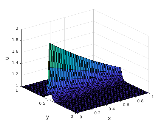
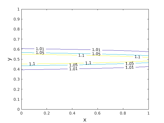
Figure 5: On the left, an example of solute concentration distribution around a fracture. On the right, the corresponding isolines.

2.3.1 Pure advection, linear reaction

In the simplified case of no diffusion, and with the advection field given by the Darcy velocity normal to the fracture, we can obtain an analytical expression for the solute concentration under the assumptions stated above. We are assuming that flux is exiting the fracture, i.e. the normal Darcy velocity $Q$ is positive and can be considered constant in time.

If we denote with $s$ the arc length in the direction normal to the fracture the one-dimensional problem for solute concentration reads:

$$\begin{aligned} &\phi{\partial_{t}u}+Q{\partial_{s}u}=-\lambda\phi u\quad&&\text{in }(0,+\infty)\times(0,T)\\ &u=u_{\gamma}&&\text{on }0\times(0,T)\\ &u(t=0)=0&&\text{in }(0,+\infty)\times\{0\}\end{aligned}$$

and has the exact solution $u(s,t)=u_{0}\left(s-{Q}t/\phi\right)\exp(-\phi\lambda/Qs)$ where

$$u_{0}=\begin{cases}u_{\gamma}&s=0\\ 0&s>0\end{cases}\quad\text{and}\quad u=\begin{cases}u_{\gamma}\exp(-\phi\lambda/Qt)&s\leq{Q}t/\phi\\ 0&s>{Q}t/\phi\end{cases}.$$

Note that, with this linear reaction term, we have precipitation whenever $u>0$, however, in practice, we can choose a cut-off value, i.e. the layer is defined by the condition $u(s,t)>\delta$.

Thus, we seek the point $\overline{s}=\epsilon_{\mu}$ where $u(\epsilon_{\mu},t)=\delta$. We obtain

$$\epsilon_{\mu}=Q/\phi\min(t,-\ln({\delta}/{u_{\gamma}})/\lambda),$$ (13)

i.e. the layer thickness grows linearly in time until it reaches its steady state value. The time to reach the steady state can be estimated as $\overline{t}=\ln({\delta}/{u_{\gamma}})/{\lambda}$.

2.3.2 A more realistic reaction term

The linear decay term considered in the previous section is however too simple for most diagenetic processes. For the case of mineral precipitation, under some simplifying assumptions, one can consider the reaction term given in (4). If we consider just the case of mineral precipitation, i.e. we assume that the solution is supersaturated, its expression simplifies to

$$r_{w}(u)=-\lambda\left(u^{2}-1\right).$$

Under the assumptions stated in the previous section, we can estimate the thickness of the layer where precipitation occurs by solving the following one dimensional problem in the direction normal to the fracture

$$\begin{aligned} &\phi{\partial_{t}u}+Q{\partial_{s}u}=-\lambda\phi\left(u^{2}-1\right)\quad&&\text{in }(0,+\infty)\times(0,T)\\ &u=u_{\gamma}&&\text{on }0\times(0,T)\\ &u(t=0)=0&&\text{in }(0,+\infty)\times\{0\}\end{aligned}.$$

At steady state, with ${\partial_{t}u}=0$, the problem above admits the exact solution

$$u(s)=\dfrac{C+\exp({2\lambda\phi s}/{Q})}{\exp({2\lambda\phi s}/{Q})-C}\quad\text{with}\quad C=\dfrac{u_{\gamma}-1}{u_{\gamma}+1}$$

to satisfy the boundary condition at the interface with the fracture. Note that, with this reaction model, precipitation only occurs where $u>1$ i.e. where the concentration is above equilibrium. Therefore we consider a cutoff value $\overline{u}=1+\delta$ with $\delta<1$ a small enough number, and seek the corresponding layer thickness

$$\dfrac{C+\exp({2\lambda\phi\epsilon_{\mu}}/{Q})}{\exp({2\lambda\phi\epsilon_{\mu}}/{Q})-C}=1+\delta\quad\Rightarrow\quad\epsilon_{\mu}=\dfrac{Q}{2\lambda\phi}\log\left(C\dfrac{2+\delta}{\delta}\right).$$ (14)

Once again the steady state layer thickness depends linearly on the ratio $Q/\lambda$. In this case however it is more difficult to obtain an expression for its growth in time: for this reason, in the results section, we will just verify this estimate and defer the actual application of this model to future work.

3 Numerical approximation

In this section we discuss the approximation strategies adopted to solve the model presented in Problem 3, in particular the spatial and temporal approximation schemes and the procedure to solve the resulting coupled and non-linear system. In Subsection 3.1 we consider the temporal discretization of the problem along with the splitting algorithm, which can be considered an extension of the one introduced and studied in [25]. In Subsection 3.2 we will briefly present the spatial discretization adopted.

3.1 Time discretization and splitting

The global physical problem, in (10), involves several processes that are coupled in a non-linear way. To overcome the need for a monolithic non-linear solver, and rely more on legacy simulation codes, suited for each single physical process, we consider a splitting strategy in time, such that each equation can be solved separately. However, we recall that the operator splitting approach usually introduces an additional error in time. Furthermore, since some of our physical variables (i.e., porosity, solute, and precipitate) are very sensitive to volume changes we also need to design the splitting strategy such that no mass or volume is unexpectedly lost. Finally, since the reaction term for the solute may be rather complex and highly non-linear, an additional operator splitting is employed to separate the diffusive and advective part from the reaction in equations (11). In this way, we can use ad-hoc numerical schemes to solve the latter.

For these reasons, we extend the strategy developed in [25] to our needs, in particular incorporating the physical processes linked to the reactive layers $\mu$. The extension is quite straightforward, however we recall the splitting algorithm for reader’s convenience. We divide the time interval in $N$ steps and we denote with $t^{n}=n\Delta t$, with $\Delta t$ the time step assumed constant for simplicity. We set the initial condition as

$$\phi^{0}_{\Omega}=\phi_{\Omega,0}\quad\epsilon^{0}_{\gamma}=\epsilon_{\gamma,0}\quad\phi^{0}_{\mu}=\phi_{\mu,0}\quad\epsilon^{0}_{\mu}=\epsilon_{\mu,0}\quad\theta^{0}_{\Omega}=\theta_{\Omega,0}\quad\theta^{0}_{\gamma}=\theta_{\gamma,0}\quad\theta^{0}_{\mu}=\theta_{\mu,0}\quad$$

$$u^{0}_{\Omega}=u_{\Omega,0}\quad u^{0}_{\gamma}=u_{\gamma,0}\quad u^{0}_{\mu}=u_{\mu,0}\quad w^{-1}_{\Omega}=w^{0}_{\Omega}=w_{\Omega,0}\quad w^{-1}_{\gamma}=w^{0}_{\gamma}=w_{\gamma,0}\quad w^{-1}_{\mu}=w^{0}_{\mu}=w_{\mu,0}.$$

In each time step $(t^{n},t^{n+1})$, we perform the following steps.

1. To get a better estimate of the porosity as well as the fracture aperture computed in the Step 2, we extrapolate the concentration of the precipitate as in [28, 2]. We obtain

   $$w^{*}_{\Omega}=2w^{n}_{\Omega}-w^{n-1}_{\Omega}\quad\text{and}\quad w^{*}_{\gamma}=2w^{n}_{\gamma}-w^{n-1}_{\gamma}\quad\text{and}\quad w^{*}_{\mu}=2w^{n}_{\mu}-w^{n-1}_{\mu}.$$

2. We then compute the porous media and layer porosity and fracture aperture, from (5) for $\phi_{\Omega}$ and $\phi_{\mu}$ and (8) for $\epsilon_{\gamma}$, by the following relations

   $$\phi_{\Omega}^{*}=\frac{\phi_{\Omega}^{n}}{1+\eta_{\Omega}(w^{*}_{\Omega}-w^{n}_{\Omega})}\quad\text{and}\quad\phi_{\mu}^{*}=\frac{\phi_{\mu}^{n}}{1+\eta_{\mu}(w^{*}_{\mu}-w^{n}_{\mu})}\quad\text{and}\quad\epsilon^{*}_{\gamma}=\frac{\epsilon^{n}_{\gamma}}{1+\eta_{\gamma}(w^{*}_{\gamma}-w^{n}_{\gamma})}.$$

   Note that we do not compute an estimate of the thickness layer $\epsilon_{\mu}$ since the models presented in Subsection 2.3 are not differential.

3. To prepare the computation of the pressure and Darcy velocity, we update the permeability of the porous media $k_{\Omega}(\phi_{\Omega}^{*})$ as well as fracture and layer permeabilities $k_{\gamma}(\epsilon^{*}_{\gamma})$ and $k_{\mu}(\epsilon^{n}_{\mu},\phi_{\mu}^{*}$, respectively.

4. We solve the Darcy problem (10) to get pressure and Darcy velocity in the domain, in the fracture and in the layer: $(\bm{q}^{n+1}_{\Omega},p^{n+1}_{\Omega})$, $(\bm{q}^{n+1}_{\gamma},p^{n+1}_{\gamma})$, and $(\bm{q}^{n+1}_{\mu},p^{n+1}_{\mu})$, respectively, as well as the interface flux $q_{\Gamma}$ on the interface $\Gamma$. For the discretization of the temporal derivative of porosity $\phi_{\Omega}$ and $\phi_{\mu}$ and fracture aperture $\epsilon_{\gamma}$ we consider both their value predicted in Step 2 and at time $n-1$.

5. We solve the advection-diffusion part of the solute equation, (11), to obtain an intermediate value of the solute: $u^{n+\frac{1}{2}}_{\Omega}$, $u^{n+\frac{1}{2}}_{\gamma}$, and $u^{n+\frac{1}{2}}_{\mu}$. Also the interface flux $\chi_{\Gamma}$ is computed on $\Gamma$. Note that we do not consider for this point the reaction term.

6. In the previous point we have accounted for porosity changes using $\phi_{\Omega}^{*}$ and $\phi_{\mu}^{*}$, as well as fracture aperture changes using $\epsilon_{\gamma}^{*}$. The intermediate value of the solute $u_{\Omega}^{n+\frac{1}{2}}$, $u_{\gamma}^{n+\frac{1}{2}}$ and $u_{\gamma}^{n+\frac{1}{2}}$ already accounts for the change in pore volume, then also the precipitate in the porous domain, fracture, and layer have to be updated to account for the same variation

   $$w^{n+\frac{1}{2}}_{\Omega}=w^{n}_{\Omega}\frac{\phi_{\Omega}^{n}}{\phi_{\Omega}^{*}}\quad\text{and}\quad w^{n+\frac{1}{2}}_{\gamma}=w^{n}_{\gamma}\frac{\epsilon^{n}_{\gamma}}{\epsilon^{*}_{\gamma}}\quad\text{and}\quad w^{n+\frac{1}{2}}_{\mu}=w^{n}_{\mu}\frac{\phi^{n}_{\mu}}{\phi^{*}_{\mu}}.$$

7. We then solve the reaction step for both the solute and precipitate, by starting from the values of $(w^{n+\frac{1}{2}}_{\Omega},w^{n+\frac{1}{2}}_{\gamma},w^{n+\frac{1}{2}}_{\mu})$ and $(u^{n+\frac{1}{2}}_{\Omega},u^{n+\frac{1}{2}}_{\gamma},u^{n+\frac{1}{2}}_{\mu})$ to get the values of $(w^{**}_{\Omega},w^{**}_{\gamma},w_{\mu}^{**})$ and $(u^{**}_{\Omega},u^{**}_{\gamma},u^{**}_{\mu})$.

8. Since the precipitate has changed in the previous step, we need to update the porosity of the porous matrix and layer as well as the fracture aperture. Considering the model (5) for $\phi_{\Omega}$ and $\phi_{\mu}$ and (8) for $\epsilon_{\gamma}$, we obtain

   $$\phi_{\Omega}^{n+1}=\frac{\phi_{\Omega}^{n}}{1+\eta_{\Omega}(w^{**}_{\Omega}-w^{n}_{\Omega})}\quad\text{and}\quad\epsilon^{n+1}_{\gamma}=\frac{\epsilon^{n}_{\gamma}}{1+\eta_{\gamma}(w^{**}_{\gamma}-w^{n}_{\gamma})}\quad\text{and}\quad\phi_{\mu}^{n+1}=\frac{\phi_{\mu}^{n}}{1+\eta_{\mu}(w^{**}_{\mu}-w^{n}_{\mu})}$$

   We also compute the thickness of the layer $\epsilon_{\mu}^{n+1}$ by following one of the model presented in Subsection 2.3.

9. As the last point in the algorithm, we update the solute and precipitate concentrations to account for the variation of porosity and fracture aperture at the previous point. We compute

   $$w^{n+1}_{\Omega}=w^{**}_{\Omega}\frac{\phi_{\Omega}^{*}}{\phi_{\Omega}^{n+1}}\quad u^{n+1}_{\Omega}=u^{**}_{\Omega}\frac{\phi_{\Omega}^{*}}{\phi_{\Omega}^{n+1}}\quad w^{n+1}_{\gamma}=w^{**}_{\gamma}\frac{\epsilon^{*}_{\gamma}}{\epsilon^{n+1}_{\gamma}}$$

   $$u^{n+1}_{\gamma}=u^{**}_{\gamma}\frac{\epsilon^{*}_{\gamma}}{\epsilon^{n+1}_{\gamma}}\quad w^{n+1}_{\mu}=w^{**}_{\mu}\frac{\phi^{*}_{\mu}}{\phi^{n+1}_{\mu}}\quad u^{n+1}_{\mu}=u^{**}_{\mu}\frac{\phi^{*}_{\mu}}{\phi^{n+1}_{\mu}}.$$

The set of ordinary differential equations to be solved in Step 7 depends on the reaction function chosen. See [34, 25, 14] for an example. For the time discretization of Step 7 in our case we have considered a second order Runge-Kutta scheme. For the other equations the first order Implicit Euler scheme is used for their temporal discretization. The operator splitting approach also introduces an error which, in our case, is of order one in time. Globally, we obtain a first order scheme in time.

3.2 Spatial discretization

The spatial discretization considered for the full problem is specific for each physical phenomenon and for each spatial dimension, since the schemes for fracture and layer are written on their tangent space. We consider schemes with compatible degrees of freedoms, meaning that they are associated only to cells (primary variables) and faces (fluxes), and no interpolation operators will be required. Since the focus of the present work is not on innovative spatial discretizations to solve the problem, but rather on the model, and since we use well known schemes, we only briefly mention them.

To compute a reliable Darcy velocity, which is then used as an input in the other problems, the numerical method has to be locally mass conservative and provide a good quality approximation of the fluxes. For this reason, our choice is to discretize the pressure equation, in its mixed form, with the lowest-order Raviart-Thomas finite element for the Darcy velocity and piece-wise constant elements for the pressure fields. This scheme is also particularly suited for strong permeability variations typical of the underground. See [36, 37, 8] for a more detailed discussion.

For the numerical solution of the solute and temperature fields, we consider a two-point flux approximation for the diffusion operator and a weighted upstream for the advective part. See [17, 39, 29] for a more extensive discussion.

The coupling between the subdomains (porous media, fracture, and layer) is done via Lagrange multipliers that represent the normal flux exchange between them. See [9, 33, 10, 29] for more details and analysis.

4 Results

In this section we present two groups of test cases to validate the previously introduced model. In the first group of test cases, in Subsection 4.1, we consider a 2D domain with one fracture, adapting the geometry of second example of [25] to our needs. In this geometry we compare the classical fracture-matrix model described in Problem 2 with the new multi-layer model in Problem 3, for increasing levels of complexity in the physical parameters. In Subsection 4.2 instead we consider a test case in three-dimensions, by adapting the geometry and data of Case 1 of [7]. In all the examples, the considered numerical scheme cannot handle the case of zero fracture aperture or layer thickness: for this reason, at the initial time when the reactive layer has not started developing yet, we will set a very low starting value for $\epsilon_{\mu}$. See [9] for a different approach that is able to handle vanishing fracture aperture. Since the presented model for the layer thickness evolution considers mostly an advective field as main driving force, we will set the diffusion coefficient for the solute transport problem to a low value to obtain results that are in agreement with the theory.

The following examples are implemented with the Python library PorePy [29] and the scripts of each test case are freely available on GitHub.

Finally, even if the current model may be coupled with a heat equation as in [25] in these experiments we consider a given, constant temperature field and therefore a fixed and uniform in space reaction rate $\lambda$.

4.1 Two-dimensional problem

In this set of tests, we consider part of the geometrical setting introduced in the second example of [25]. We refer to Table 1 for a list of the data and physical parameters common to the three cases presented in this section. The porous medium, represented by the domain $\Omega=(0,1)^{2}$, is partially cut by a single fracture $\gamma=\{(x,y)\in\Omega:\,y=x-0.1,x\leq 0.9\}$ with the surrounding layers $\mu$, which geometrically coincide with $\gamma$. See Figure 6 for a graphical representation.

$\delta=0.1$	$\phi_{\Omega,0}=0.2$	$\phi_{\mu,0}=0.2$	$\epsilon_{\gamma,0}=10^{-3}$	$\epsilon_{\mu,0}=10^{-8}$
$k_{0}=1$	$k_{\gamma,0}=10^{2}$	$\kappa_{\gamma,0}=10^{2}$	$k_{\mu,0}=1$	$\kappa_{\mu,0}=1$
$\mu=1$	$f=0$	$f_{\gamma}=0$	$f_{\mu}=0$	$q_{\partial\Omega}^{\rm no-flow}=0$
$p_{\partial\Omega}^{\rm out-flow}=0$	$p_{\partial\Omega}^{\rm in-flow}=1$	$p_{\partial\gamma}^{\rm in-flow}=10^{-1}$	$p_{\partial\mu}^{\rm in-flow}=10^{-1}$	$d=10^{-8}$
$d_{\mu}=10^{-6}$	$\delta_{\mu}=10^{-6}$	$d_{\gamma}=10^{-6}$	$\delta_{\gamma}=10^{-6}$	$u_{\Omega,0}=0$
$\chi_{\partial\Omega}^{\rm no-flow}=0$	$u_{\partial\Omega}^{\rm in-flow}=2$	$u_{\partial\Omega}^{\rm out-flow}=0$	$u_{\gamma,0}=0$	$u_{\partial\gamma}^{\rm in-flow}=2$
$u_{\mu,0}=0$	$u_{\partial\mu}^{\rm in-flow}=2$	$\lambda^{-}=100$	$r(u)=u$

Table 1: Common data for the examples in Subsection 4.1.

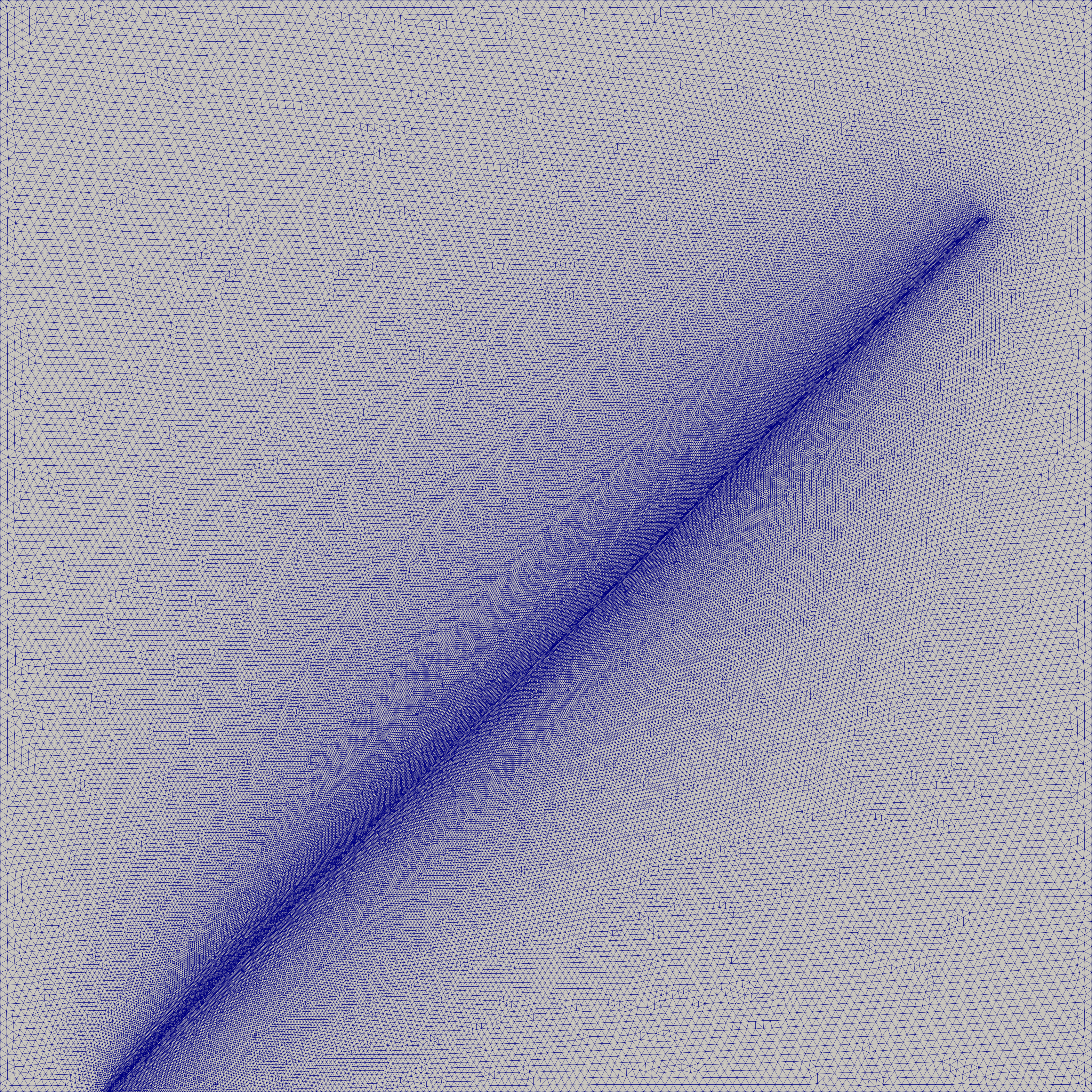
Figure 6: On the left, domain $\Omega$, fracture $\gamma$, and the two sides of the layer $\mu$ for the cases of Subsection 4.1. At the center the computational grid used for the multi-layer model and on the right the finer computational grid used for the simulation of the fracture-matrix model (without the layer).

One of the main criteria in our evaluation, apart from a graphical observation of the solution, is the comparison between the thickness of the layer $\mu$ estimated with model in Problem 3 and the one obtained from the simulation of the matrix-fracture Problem 2 as in [25], with a grid fine enough to capture the concentration gradients around the fracture. This latter high resolution simulation will numerically validate the accuracy of the proposed model in this setting. Clearly, both test cases in this section deviate from the assumptions at the basis of the theoretical model for the layer thickness (13): the transport of solute from the fracture is not exactly one-dimensional, there is a small diffusive effect, and, if porosity is allowed to change due to precipitation, the Darcy velocity cannot be considered constant. Our aim is to test the robustness of the model prediction for different cases, to establish its usefulness in realistic situations.

The simulation has $100$ time steps of equal length, with ending time $T_{f}=0.2$. For the multi-layer model we consider a uniformly refined mesh of 38435 triangles for the porous media, 290 segments for the layer and 145 segments for the fracture, while for the model where only the fracture is a lower dimensional object, we have considered a very fine grid around the fracture itself which gives a non-uniform triangular grid composed of 107841 elements. The fracture is discretized with 906 equal segments. See Figure 6 for the graphical representation of the computational grids.

4.1.1 Case 1

For this case we consider the data and geometry describe above, and we additionally set the following parameters: $\eta_{\Omega}=0$, $\eta_{\gamma}=0$, and $\eta_{\mu}=0$ thus the porosity $\phi_{\Omega}$ and $\phi_{\mu}$, as well as the fracture aperture $\epsilon_{\gamma}$, are fixed for the entire simulation and are equal to their initial value. In this case the Darcy velocity $\bm{q}$ is constant in time in the entire domain (although not necessarily exactly normal to the fracture).

       
              
              

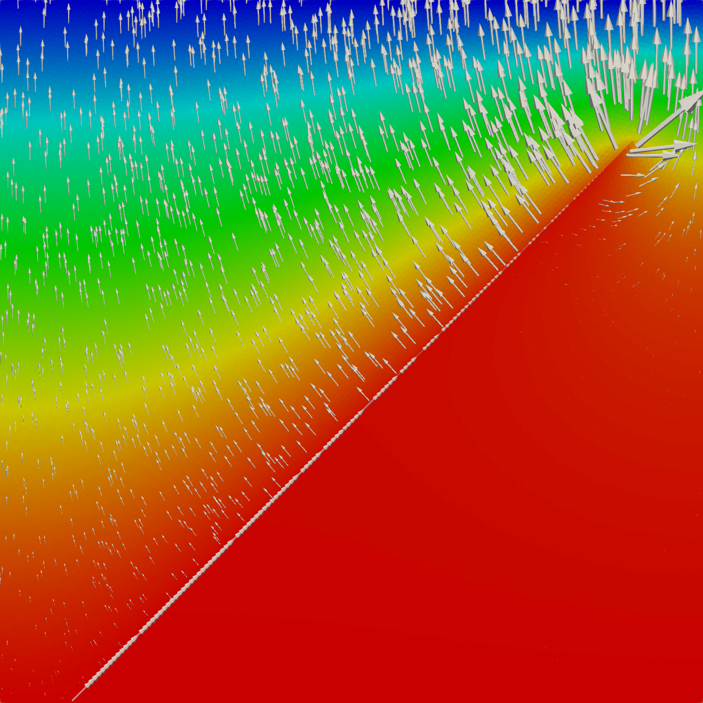
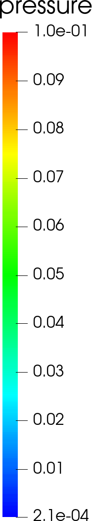
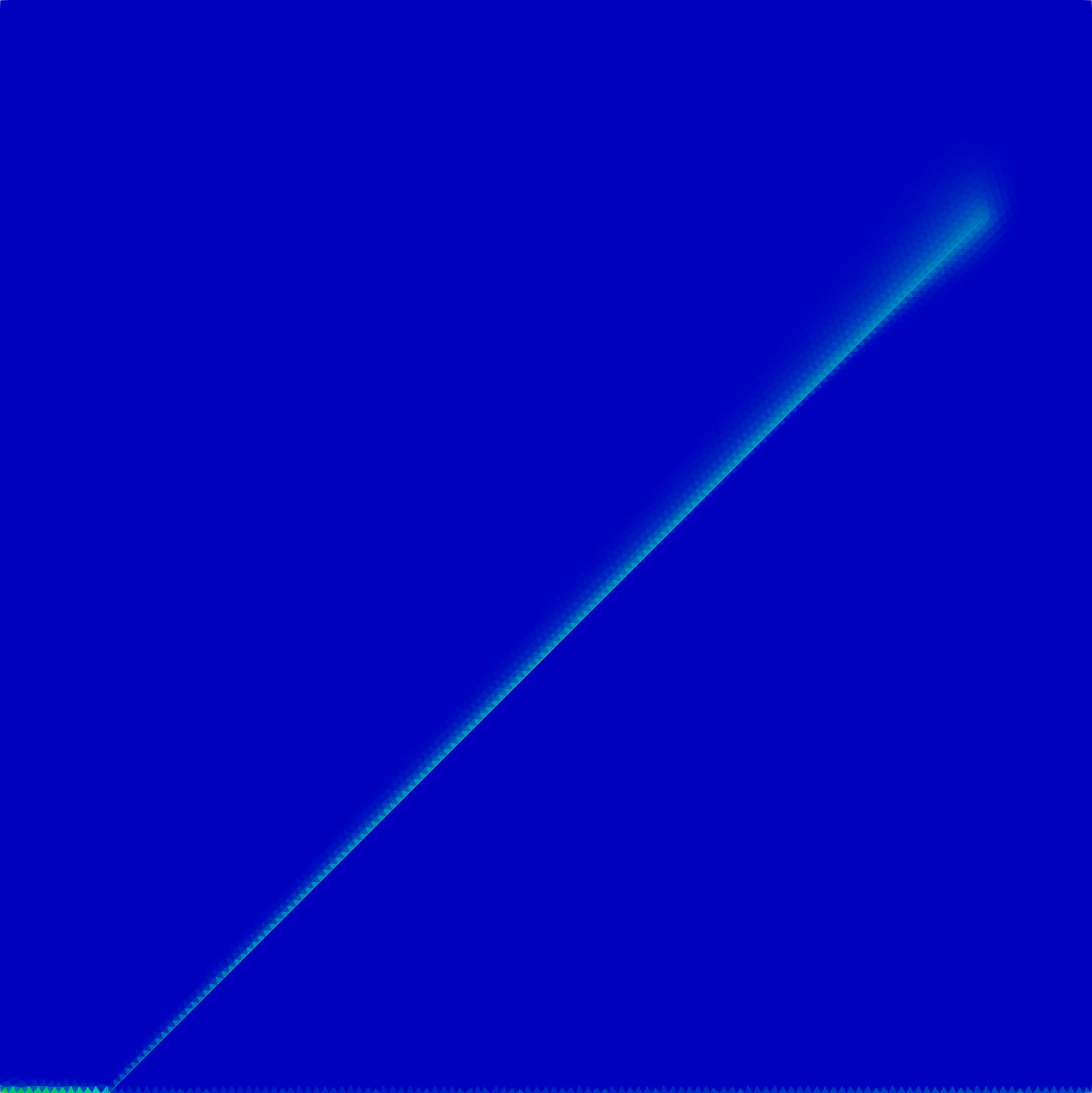
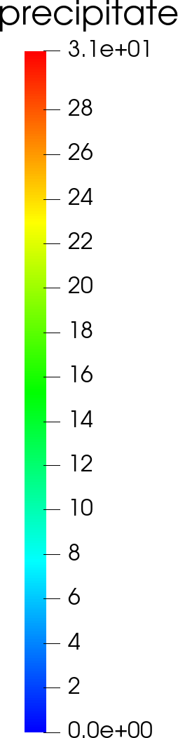
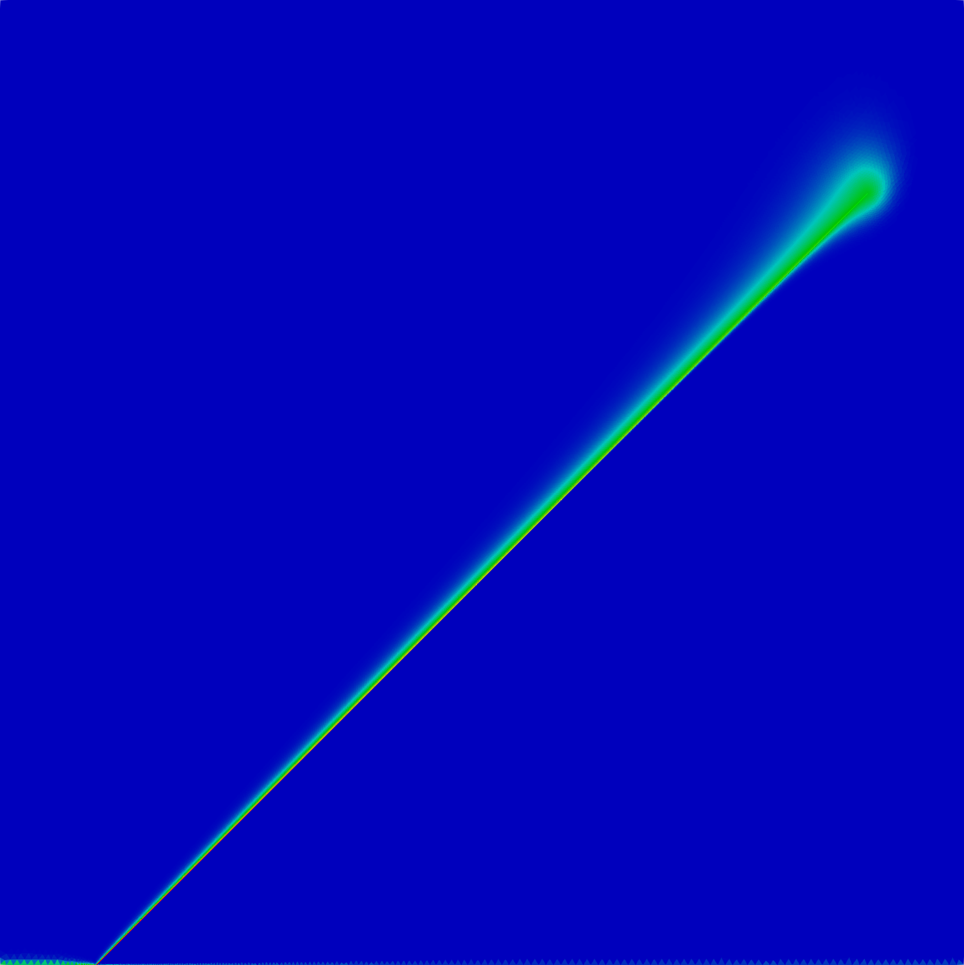
Figure 7: Graphical representation of the pressure (top), solute (centre), and precipitate (bottom) for the test case described in Sub-subsection 4.1.1 at the end of the simulation. On the left for the multi-layer reduced model in Problem 3 and on the right for the matrix-fracture model in Problem 2.

In Figure 7 we compare the pressure and Darcy velocity, along with the solute and precipitate obtained with the two models and corresponding discretizations. First of all let us note that, since $\eta_{\Omega}$ is null, pressure and Darcy velocity are fixed in time The solution shows the advantage of adopting the introduced model, since we can observe that with a fast enough reaction most of the dynamics for the solute and precipitate develops very close to the fracture $\gamma$. The graphical difference in the solute and precipitate distribution is mainly due to the fact that, in the multi-layer model, the part of the solution with the higher concentrations is represented by the reduced variables $u_{\mu}$, $w_{\mu}$ in the one-dimensional layers.

       

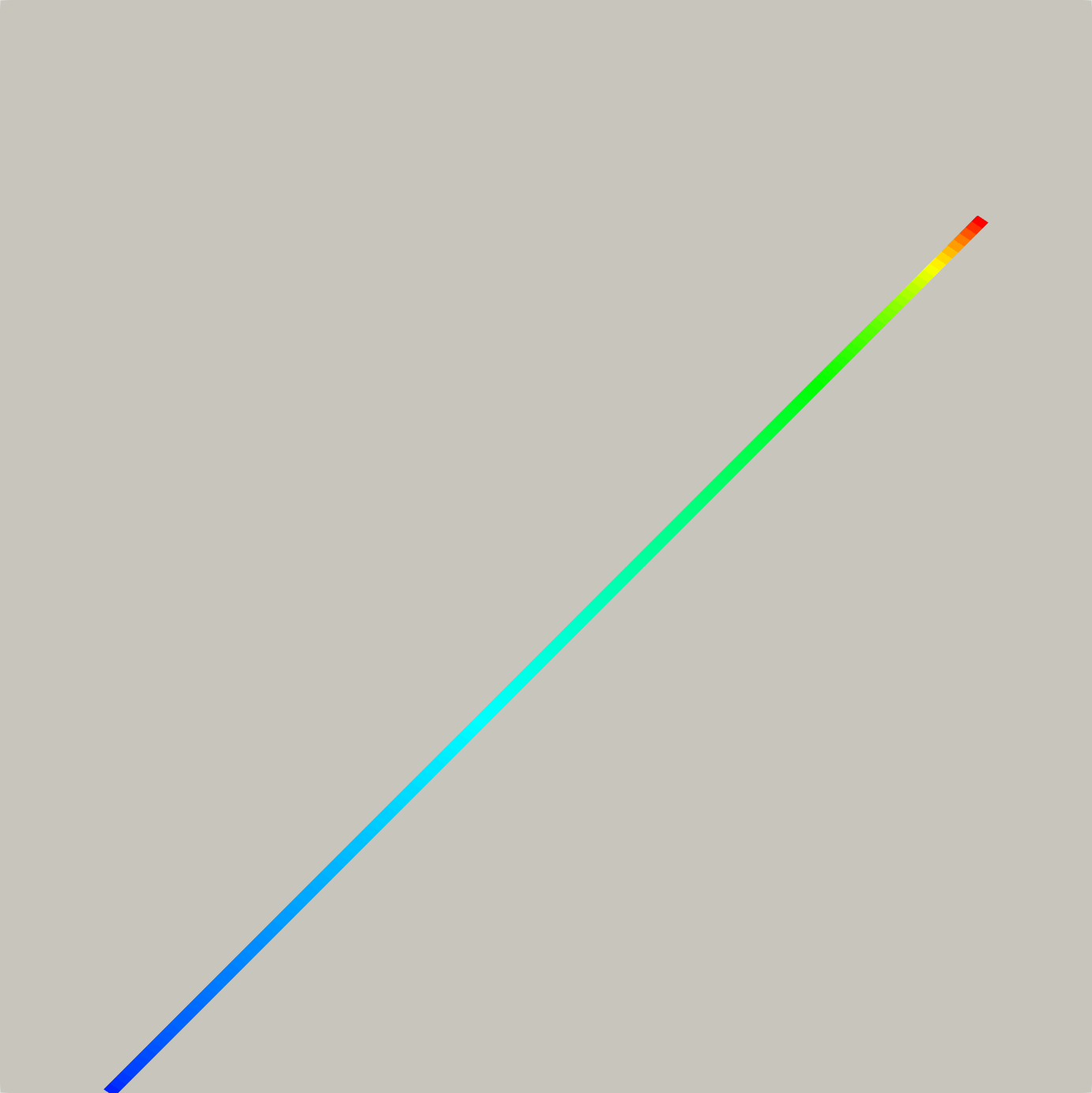
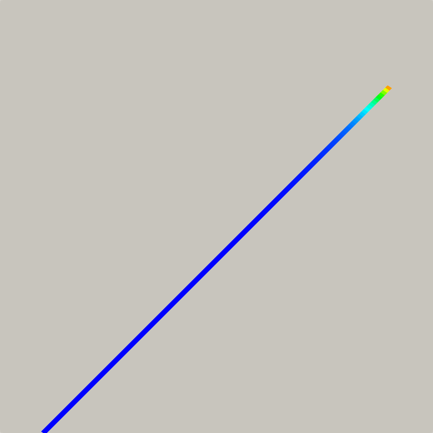
Figure 8: Layer thickness for both sides (top layer on the left, bottom layer on the right) at the end of the simulation time for the test case in Sub-subsection 4.1.1.

In Figure 8 we see the layer thickness at the end of the simulation. Since it depends on the Darcy velocity at fracture-layer interface, the top part of the layer (the one closer to the outflow) is wider than on the bottom part. For both sides, at their tip the aperture results in a much higher value due to the outflow from the fracture tip. Given the small layer thickness, we can consider the proposed model to be in its range of applicability, i.e. the layers can be reduced to their center line.

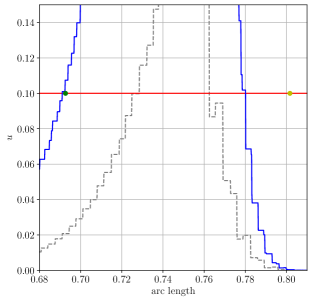
Figure 9: Profile of the solute along two lines normal to the fracture, $l_{1}$ on the left and $l_{2}$ on the right. The blue line represent the solute profile obtained with the proposed multi-layer model, while the red line with the equi-dimensional layers $\mu$ and a fine grid. The green and yellow dot represent the point $(a^{\pm}\pm\epsilon_{\mu}^{\pm},\delta)$ for the top and bottom layer respectively. Results for the test case in Sub-subsection 4.1.1.

Finally, Figure 9 shows the graphical comparison between the solute along two specifics lines normal to the fracture: $l_{1}$ which connects $(0,1)$ and $(1,0)$, crossing the fracture at $(0.5,0.5)$ and layers, and $l_{2}$ which connects $(0.3656,1.3293)$ and $(1.3658,0.3293)$, passing close to the fracture tip. The concentration profiles computed with the matrix-fracture and the multi-layer models are plotted against the arc curve length coordinate along $l_{1}$ and $l_{2}$. These profiles are compared with the layer thickness predicted by (13), marked by the dots in position $(a_{1,2}\pm\epsilon_{\mu}^{\pm},\delta)$, where $a_{1}=0.778$ (for line $l_{1}$) and $a_{2}=0.7521$ (line $l_{2}$) are the intersections with the fracture. These dots correspond to the point where solute concentration drops below the cutoff value ($\delta=0.1$), and thus mark the border of the layer $\mu^{\pm}$.

We can notice that for $l_{1}$ the results are in good agreement, while for $l_{2}$ we get accurate results only for the top part of the layer. For the bottom part of $\mu$ on its tip, the model assumption that the flow is mostly normal however, in this particular case, is not valid since the outflow from the fracture tip creates strongly bidimensional effects in the solution.

We can conclude that, in this setting, the multi-layer reduced model is an attractive and effective alternative which gives coherent results with the model of [25].

4.1.2 Case 2

In this second test case of the group, we allow for a more complex physical interaction between the variables by setting $\eta_{\Omega}=5\cdot 10^{-2}$, $\eta_{\gamma}=5\cdot 10^{-2}$, and $\eta_{\mu}=5\cdot 10^{-2}$: thus, the porosity and consequently then the permeability change in time and alter pressure and Darcy velocity fields. The problem becomes more coupled. We would like to understand if the presented model gives reasonably accurate outcomes even if this setting does not satisfy the hypotheses at the basis of the derived layer evolution (even more than the previous case).

Let us consider a graphical comparison of the solution obtained with the two models, reported in Figure 10.

       
              
              

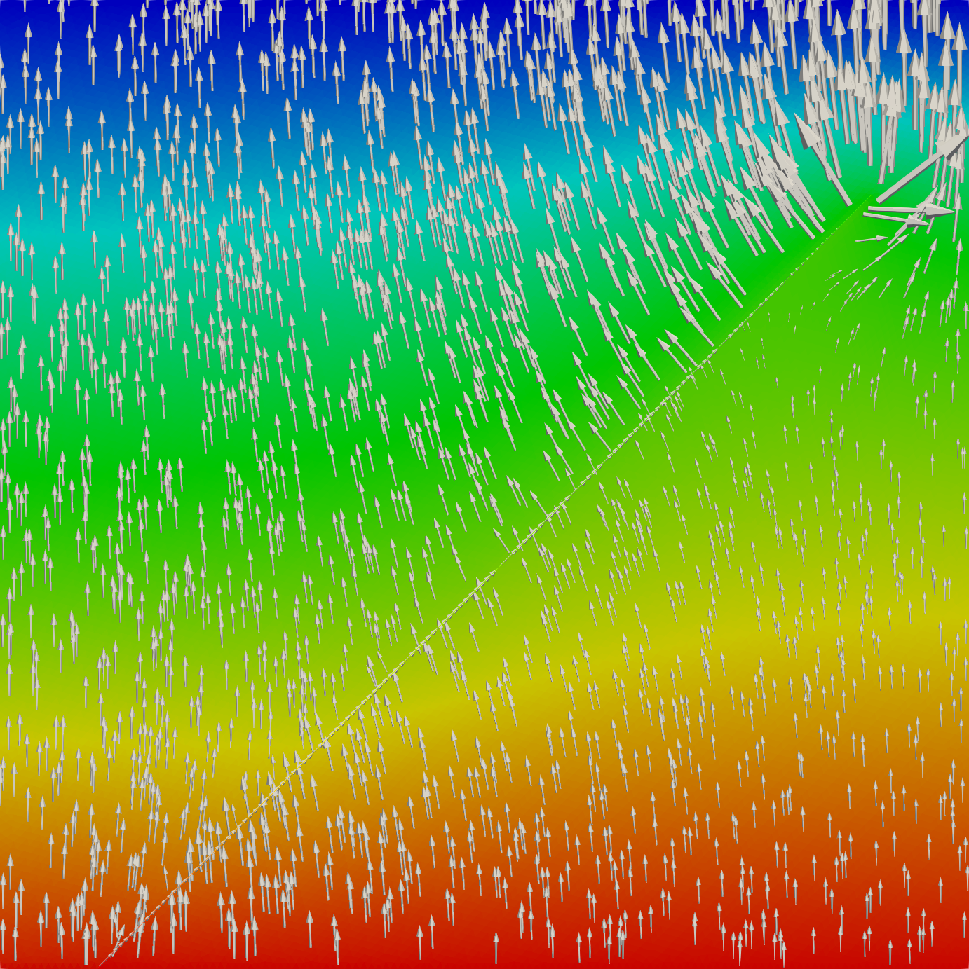
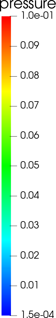
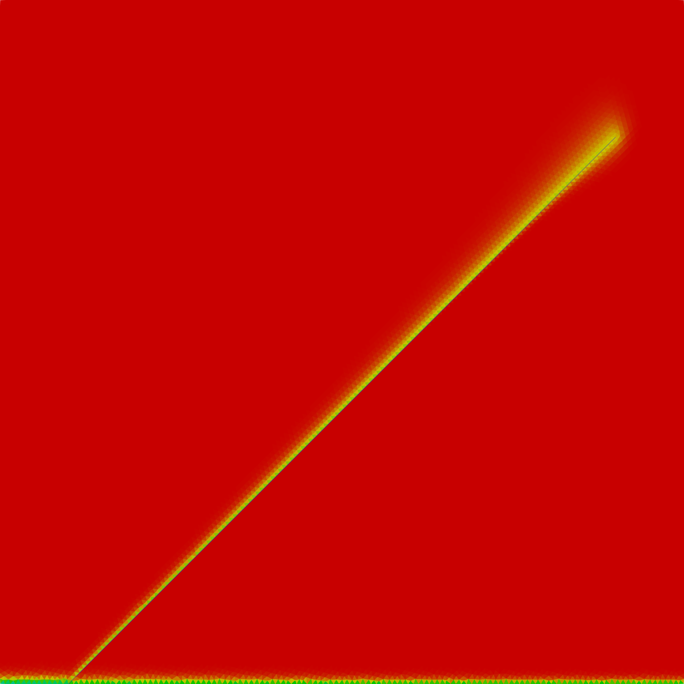
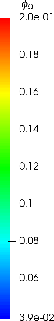
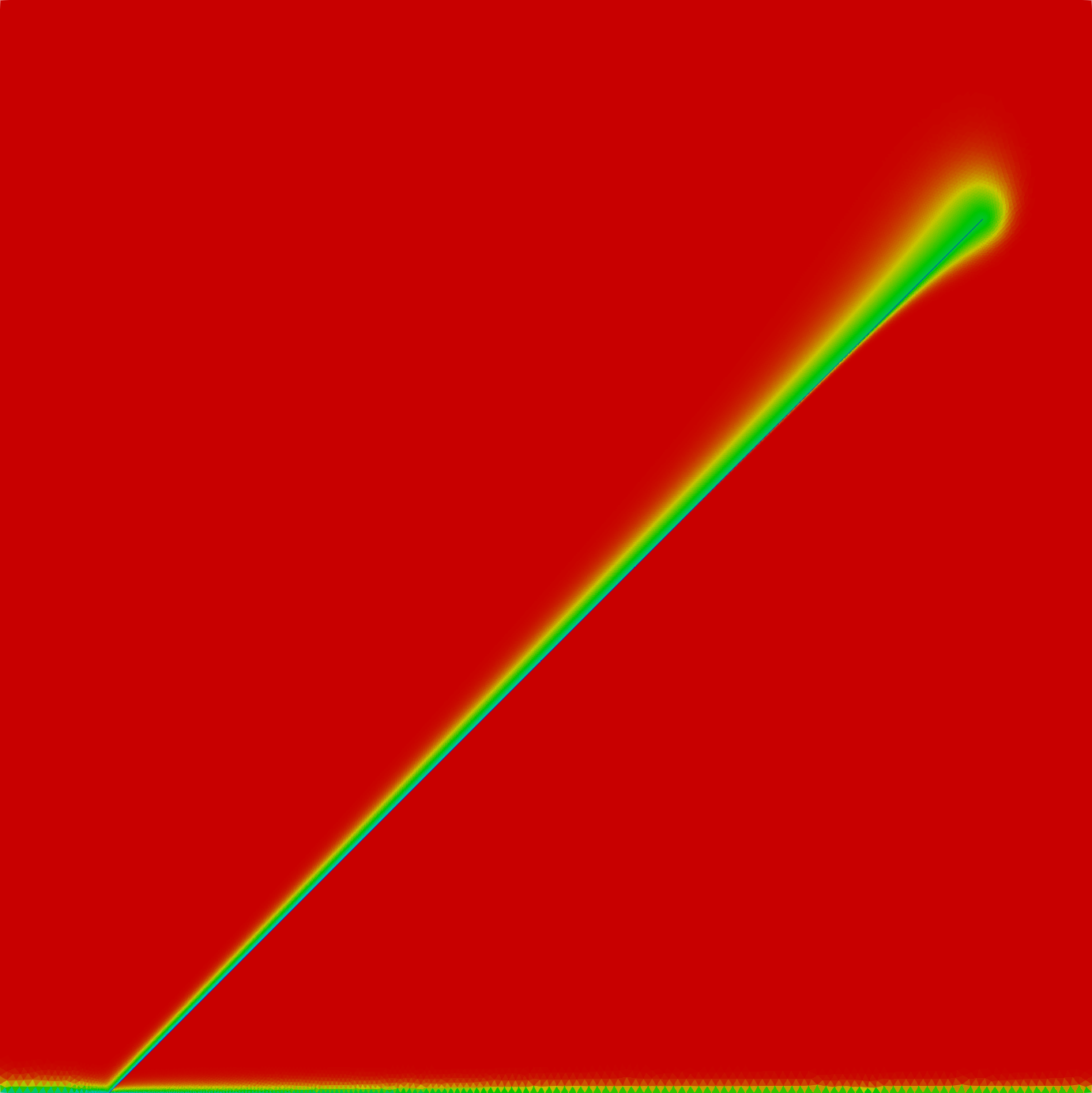
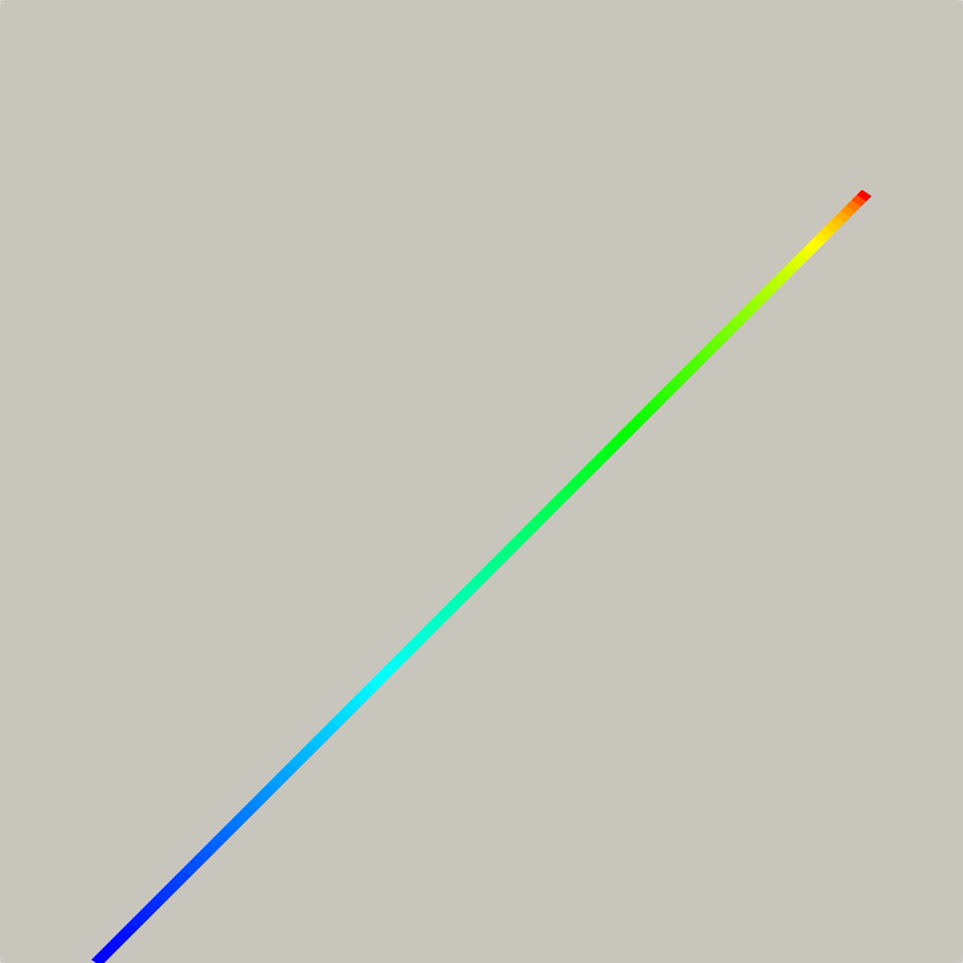
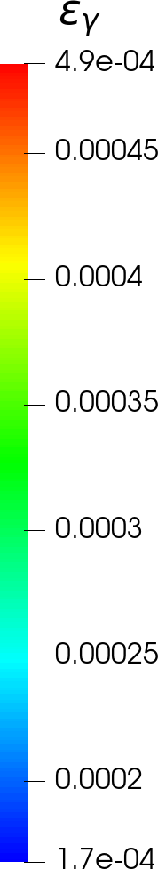
Figure 10: Graphical representation of the pressure (top), porosity (centre), and fracture aperture (bottom) for the test case described in Sub-subsection 4.1.2 at the end of the simulation. On the left for the multi-layer reduced model in Problem 3 and on the right for the matrix-fracture model in Problem 2.

Comparing the pressure profile with the one obtained in the test case of Sub-subsection 4.1.1, we clearly see the effect of the $\eta$ parameters on porosity and fracture aperture. The fracture indeed now becomes less permeable (due to its shrinking aperture) as well as the layer surrounding it (due to decreasing porosity).

We note that the predicted and observed thickness of the layer is such that, also in this case, it is beneficial to adopt a multi-layer approach. We notice also that the fracture aperture is smaller closer to the inflow of the problem: this is due to the solute that enters the domain, flows mainly into the fracture and precipitates there, altering its aperture. This results in a slower fracture flow which in turn affects the overall process.

       
              

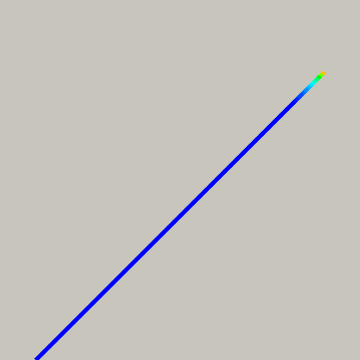
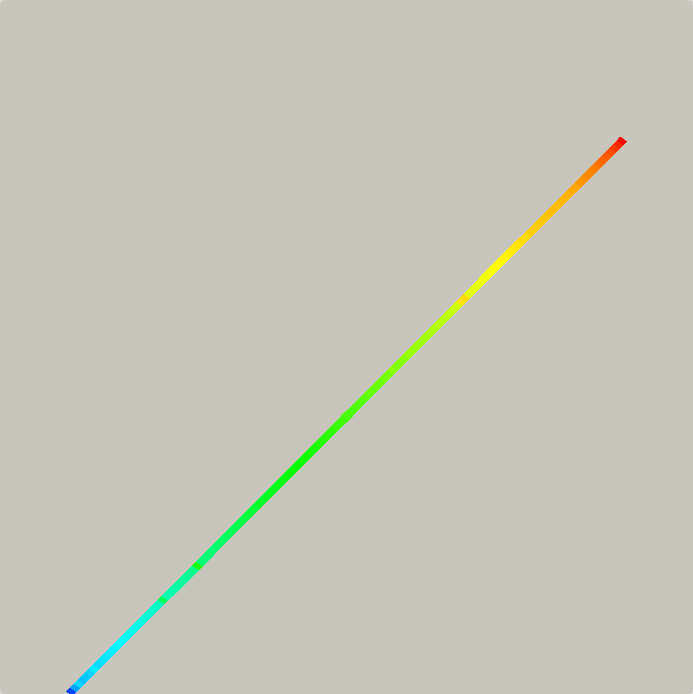
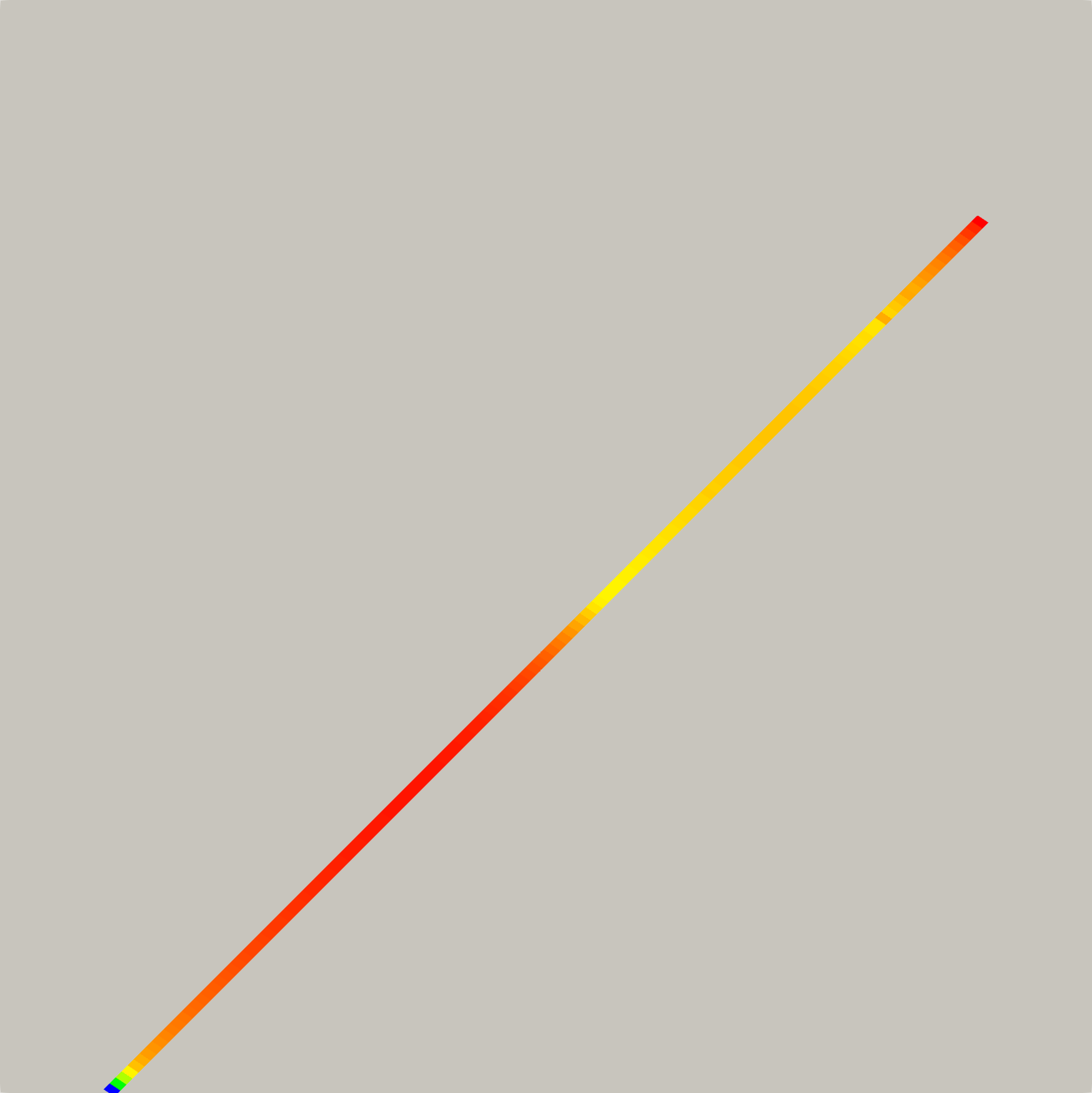
Figure 11: Layer thickness for both sides (top layer on the left, bottom layer on the right) at the end of the simulation time for the test case in Sub-subsection 4.1.2.

Figure 11 represents the layer thickness and porosity at the end of the simulation. The difference between the two sides is evident, mainly due to the difference in the flow exiting the fracture on the two sides.

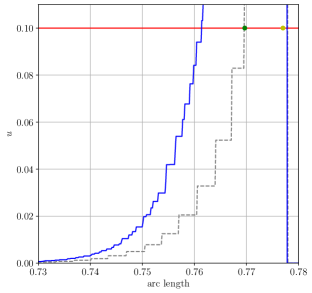
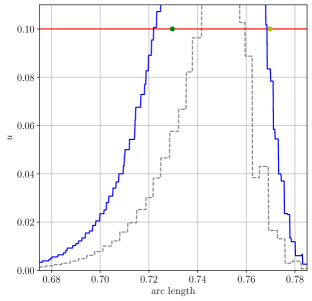
Figure 12: Profile of the solute along two lines normal to the fracture, $l_{1}$ on the left and $l_{2}$ on the right. The blue line represent the solute profile obtained with the proposed multi-layer model, while the red line with the equi-dimensional layers $\mu$ and a fine grid. The green and yellow dot represent the point $(a_{1,2}\pm\epsilon_{\mu}^{\pm},\delta)$ for the top and bottom layer respectively. Results for the test case in Sub-subsection 4.1.2.

Finally, in Figure 12 we compare the solute on the same lines specified in the previous Sub-subsection 4.1.1, $l_{1}$ and $l_{2}$. The model for the thickness layer prediction is now slightly less accurate then before, due to the effect of the not null $\eta$ parameters, however we still find good qualitative agreement between the results.

We can conclude that, also in this setting, the multi-layer reduced model is able to represent the effects quite accurately with a much lighter computational cost than a refined grid, even if we are outside of the assumptions for the layer thickness evolution.

4.1.3 Case 3

In this example we consider the same data of Case $1$ in Sub-subsection 4.1.1 but the reaction rate is now modeled with a non-linear function of the solute. We set $r(u)=u^{2}$, $r_{w}(u)=-\lambda\max\left(u^{2}-1,0\right)$. In this case we will note that precipitation occurs only if $u$ exceeds $1$, the non-dimensional equilibrium value.

The aim of this test is to validate the formula (14) for the prediction of the layer thickness. Since this expression is derived only for the steady state and not for the actual evolution of $\epsilon_{\mu}$, we cannot run the multi-layer model in Problem 3 but only the fracture-matrix Problem 2 and observe whether the solute/precipitate distribution corresponds to our predictions. The use of this reaction rate in the multi-layer model would require the derivation of an expression or an approximation of the layer thickness in time, which will be the subject of future work.

Due to the chosen data, since $\eta=0$, the porosity and fracture aperture are fixed at their initial value and thus the pressure field and Darcy velocity are the same as in Case $1$, and represented on the top of Figure 7. The solute and precipitate in the rock matrix are represented in Figure 13, which shows for both fields the existence of a narrow region surrounding the fracture with very different values than the remaining part of the rock matrix. This justifies once again the necessity to adopt a reduced model to describe the layer around the fracture. Moreover, note that further away form the fracture the solute concentration is below the equilibrium value ($u=1$) therefore no precipitation occurs.

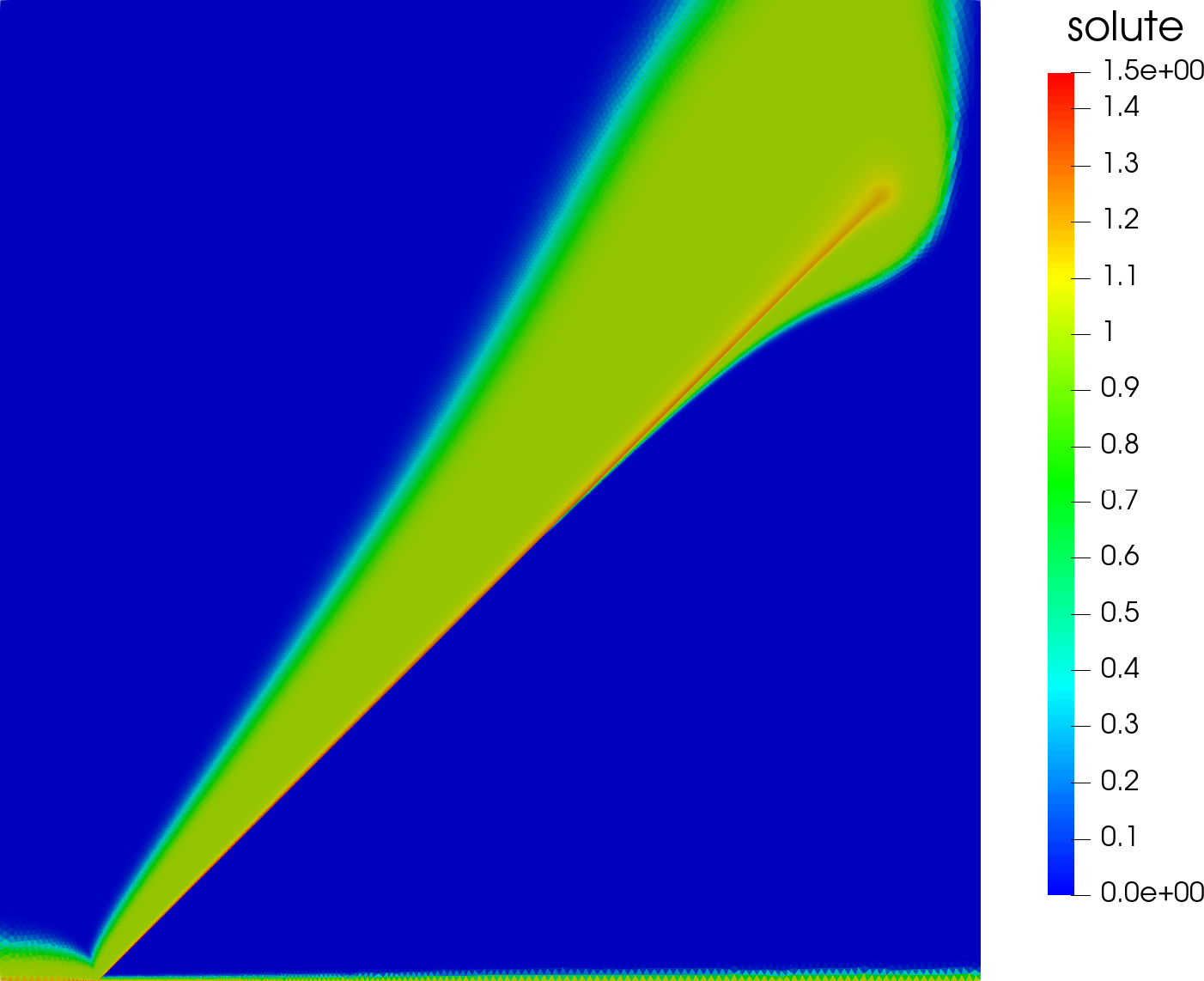
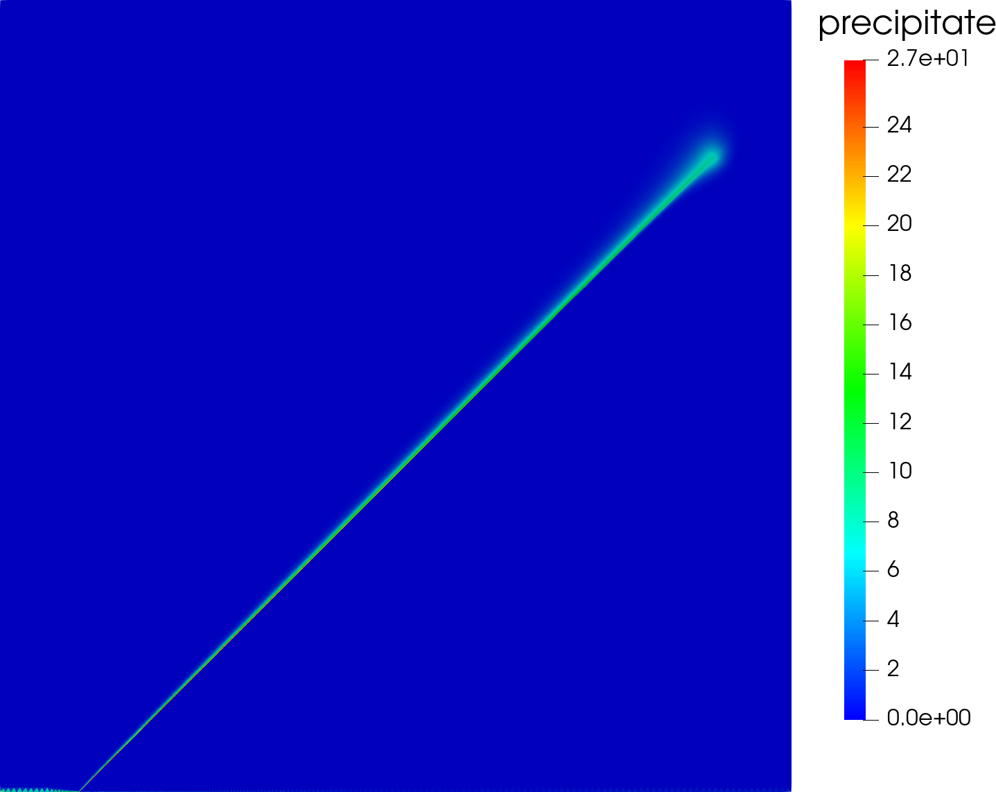
Figure 13: Solute and precipitate in the rock matrix at the end of the simulation time for the test case in Sub-subsection 4.1.3.

Figure 14 shows the comparison between the layer thickness predicted with (14) and the one graphically estimated from the numerical results of model in Problem 2. For the comparison we consider again the lines $l_{1}$ and $l_{2}$ introduced previously. First of all, on both lines we can observe a peak in the solute profiles in correspondence of the fracture. The value of solute concentration then decreases quickly reaching the plateau value $u=1$. As done in the previous cases we can compare the predicted layer thickness, according to (14), with the numerical results: this time the dots correspond to the points in position $(a_{1,2}\pm\epsilon_{\mu}^{\pm},1+\delta)$, where $a_{1}=0.778$ (for line $l_{1}$) and $a_{2}=0.7521$ (line $l_{2}$) and $\delta=0.1$. We can observe a good agreement between the predicted and measured layer size in both cases, even close to the fracture tip.

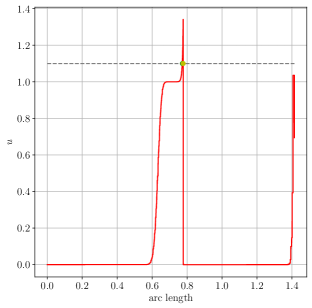
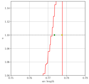
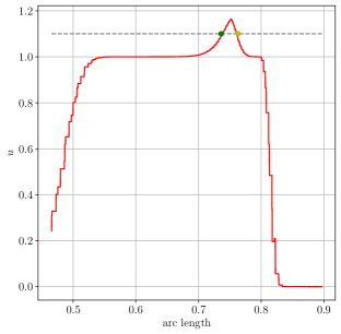
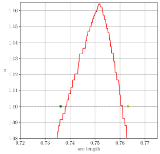
Figure 14: Profile of the solute along two lines normal to the fracture, $l_{1}$ on the top and $l_{2}$ on the bottom. On the right a zoom around the estimated values. The red line represent the solute profile obtained with the equi-dimensional layers $\mu$ and a fine grid. The green and yellow dot represent the point $(a_{1,2}\pm\epsilon_{\mu}^{\pm},\delta+1)$ for the top and bottom layer respectively. Results for the test case in Sub-subsection 4.1.3.

Even if for the non-linear case more analysis should be done, these results can be considered promising and they confirm the feasibility of adopting a reduced model for the layer $\mu$ around the fracture.

4.2 Three-dimensional problem

For this test case we consider a three dimensional setting inspired from the Case 1 of [7]. In particular, we adopt the same geometry and part of the data for the flow problem at the outset of the simulation. The aim of this test case is to validate the proposed model in Problem 3 in a three-dimensional setting. Referring to Figure 15, the bottom part of the domain has higher porosity and permeability than the remaining part. We note that the inflow part of the boundary is slightly larger that the one in [7] to allow direct inflow into the fracture and layer, and thus obtain a simpler flow pattern around the fracture that fits the assumptions of our model.

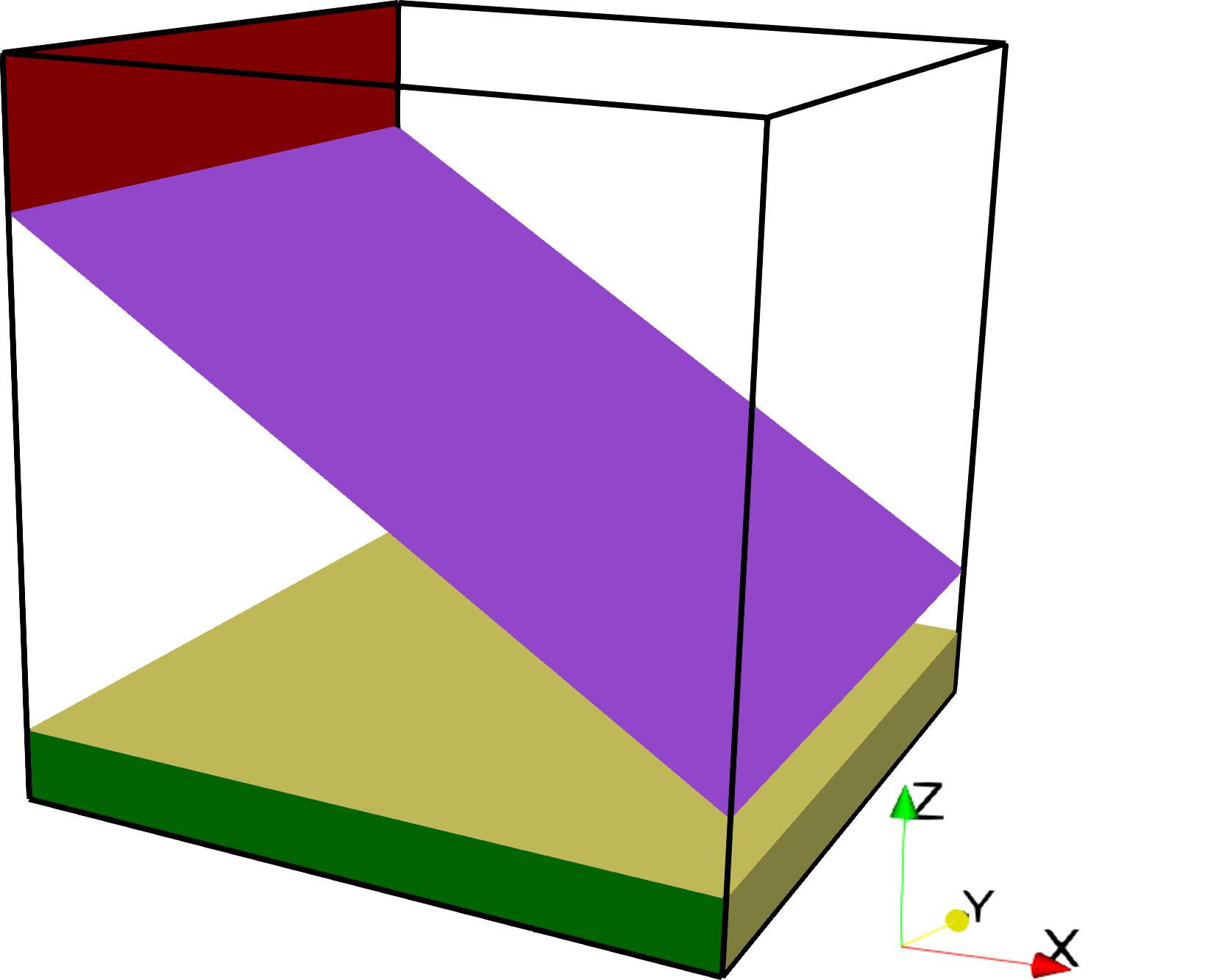
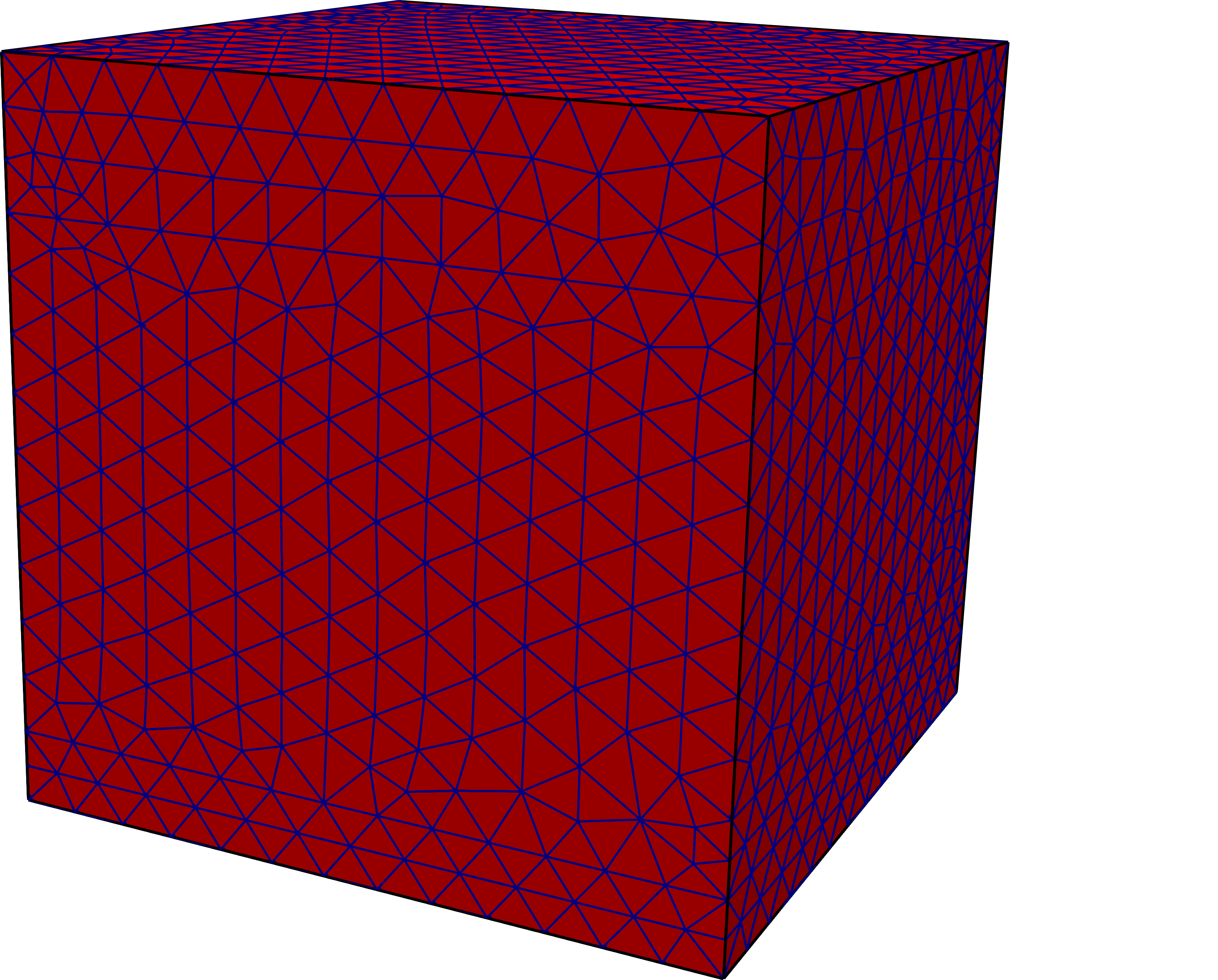
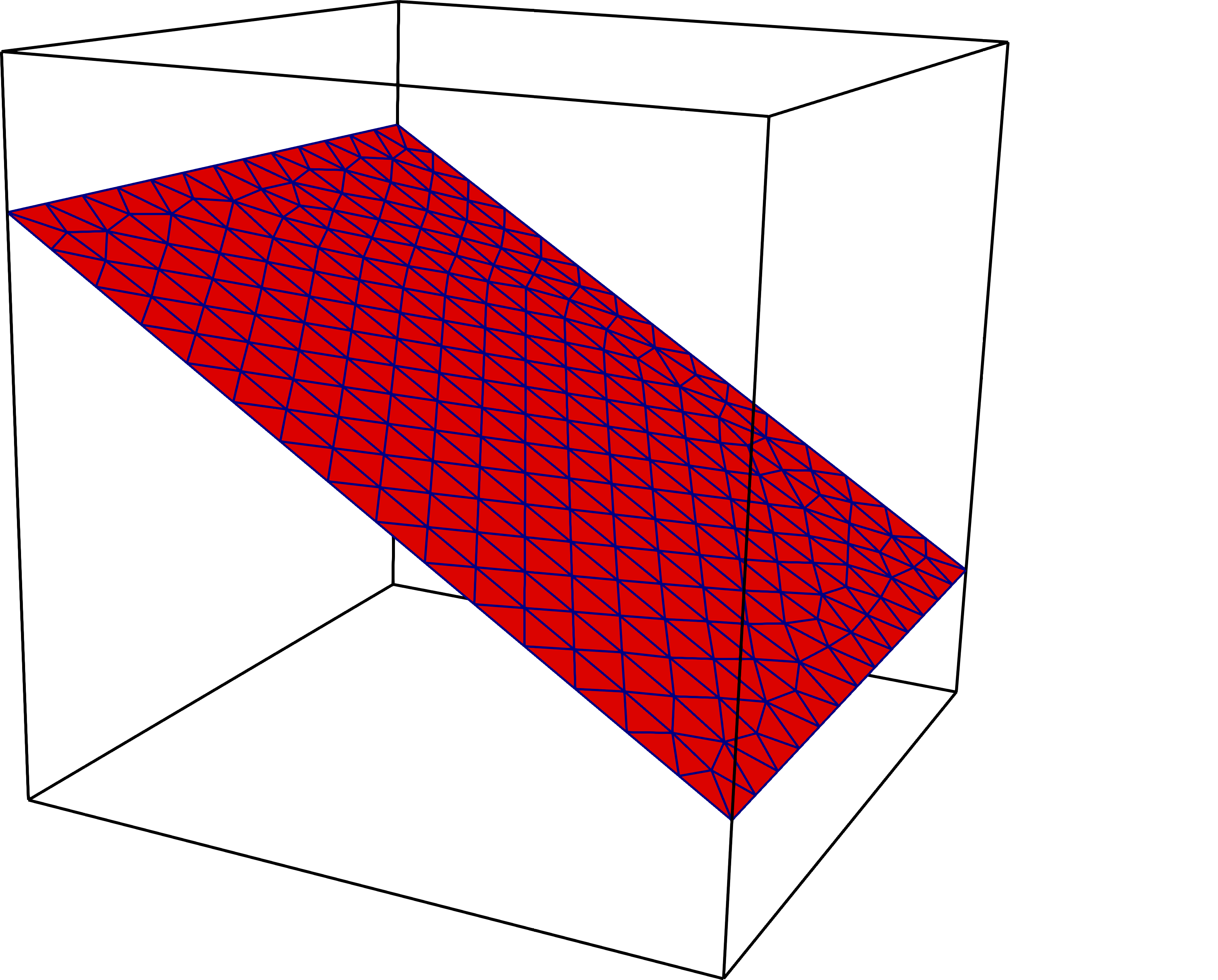
Figure 15: Computational domain for the test case in Subsection 4.2. The magenta represents the fracture and the layer, the red part is the inflow boundary region while the green is the outflow. Finally, the yellow block is the part with different matrix porosity and permeability.

For the data used in the simulation see Table 2.

cutoff $=0.1$	$\phi_{\Omega,0}^{\rm low}=0.2$	$\phi_{\Omega,0}^{\rm high}=0.25$	$\phi_{\mu,0}=0.25$	$\epsilon_{\gamma,0}=4\cdot 10^{-3}$
$\epsilon_{\mu,0}=10^{-8}$	$k_{0}^{\rm low}=10^{-6}$	$k_{0}^{\rm high}=10^{-5}$	$k_{\gamma,0}=10^{-1}$	$\kappa_{\gamma,0}=10^{-1}$
$k_{\mu,0}=10^{-5}$	$\kappa_{\mu,0}=10^{-5}$	$\mu=1$	$f=0$	$f_{\gamma}=0$
$f_{\mu}=0$	$q_{\partial\Omega}^{\rm no-flow}=0$	$p_{\partial\Omega}^{\rm out-flow}=1$	$p_{\partial\Omega}^{\rm in-flow}=4$	$q_{\partial\gamma}^{\rm no-flow}=0$
$q_{\partial\mu}^{\rm no-flow}=0$	$d=10^{-12}$	$d_{\mu}=10^{-12}$	$\delta_{\mu}=10^{-12}$	$d_{\gamma}=10^{-12}$
$\delta_{\gamma}=10^{-12}$	$u_{\Omega,0}=0$	$\chi_{\partial\Omega}^{\rm no-flow}=0$	$u_{\partial\Omega}^{\rm in-flow}=2$	$u_{\partial\Omega}^{\rm out-flow}=0$
$u_{\gamma,0}=0$	$\chi_{\partial\gamma}^{\rm no-flow}=0$	$u_{\partial\gamma}^{\rm in-flow}=2$	$u_{\mu,0}=0$	$\chi_{\partial\mu}^{\rm no-flow}=0$
$u_{\partial\mu}^{\rm in-flow}=2$	$\lambda^{-}=10^{-6}$	$r(u)=u$	$\eta_{\Omega}=0.5$	$\eta_{\gamma}=0.5$
$\eta_{\mu}=0.5$

Table 2: Data for the examples in Subsection 4.2.

The computational grid is composed of 11436 tetrahedra for the porous media, 470 triangles for the fracture and 940 triangles for the layer. The final simulation time is $5\cdot 10^{5}$ divided uniformly in 100 time steps. We note that the final time is shorter than in [7] since most of the dynamic of our interest happens at an early stage.

Figure 16 shows the pressure and solute in the rock matrix at the end of the simulation time. We notice that the fracture remains highly conductive and also that the solute in the rock matrix is quite low. Indeed, at the end of the simulation time, most of the dynamics happened only in the fracture and surrounding layer.

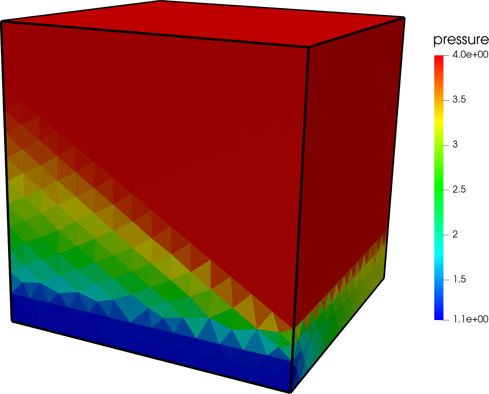
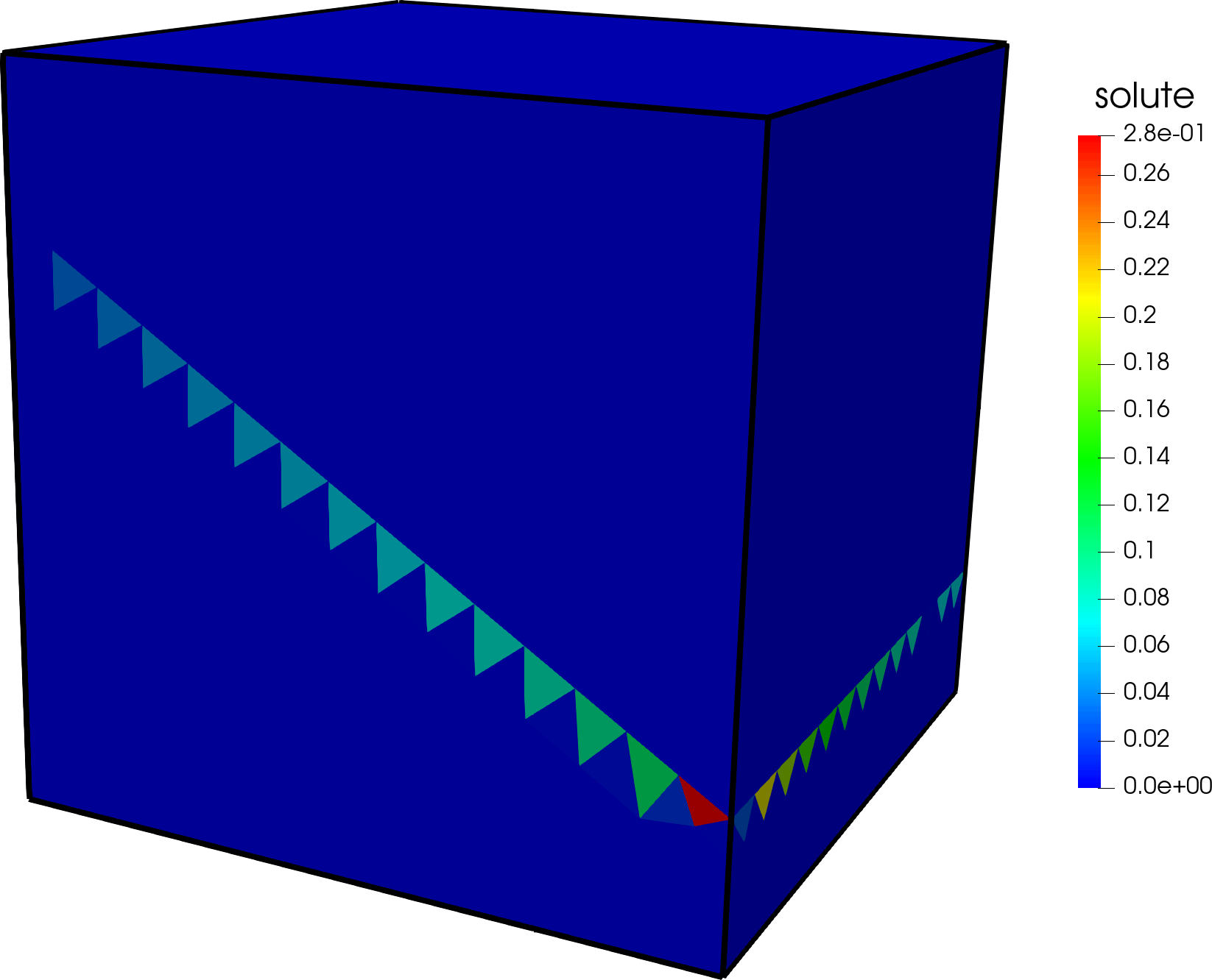
Figure 16: On the left, the pressure field and, on the right, the solute for the test case in Subsection 4.2.

In Figure 17 we represent the fracture aperture and solute at the end of the simulation time. As noted before, the fracture remains highly conductive and the inflow concentration of the solute is transported quickly in the whole fracture. This also implies also precipitation inside the fracture and thus fracture aperture variation, as well as a strong influence on the layer thickness evolution.

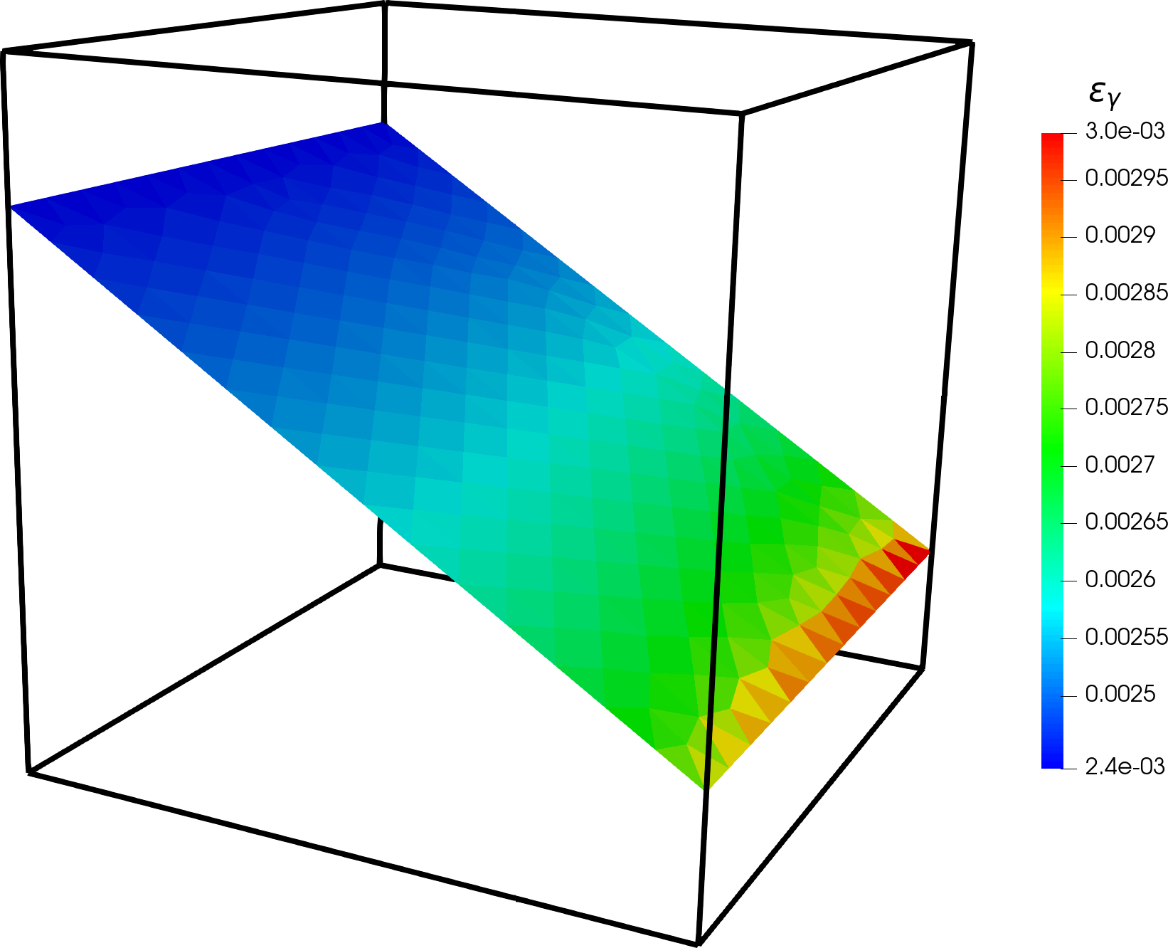
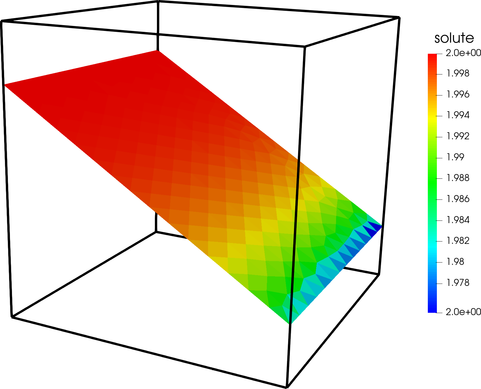
Figure 17: On the left, the fracture aperture and, on the right, the fracture solute for the test case in Subsection 4.2.

Figure 18 show the dynamics inside the layer. We obtain more precipitate in the top part of the layer $\mu$ due to the inflow into the layer itself from the top part of the rock matrix, and also because, in the bottom part of $\mu$, the solute tends to flow towards the outflow boundary at the bottom, resulting in a smaller concentration of precipitate in the bottom part of $\mu$. The layer thickness is also represented, with two different scales, overlapped with the Darcy velocity in the fracture, as a proxy for the flow exchange between the fracture and the layer. We see that the top part of the layer is rather thin and in principle might be neglected, however on the bottom part a higher value of the thickness reveals the importance of having the layer explicitly represented. The aperture in this case is not uniform, but rather, larger near the outflow of the problem, as one could expect.

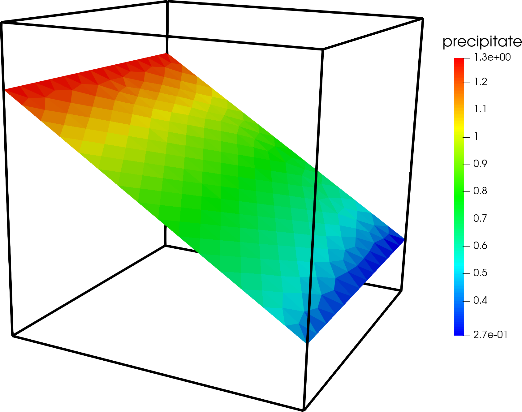
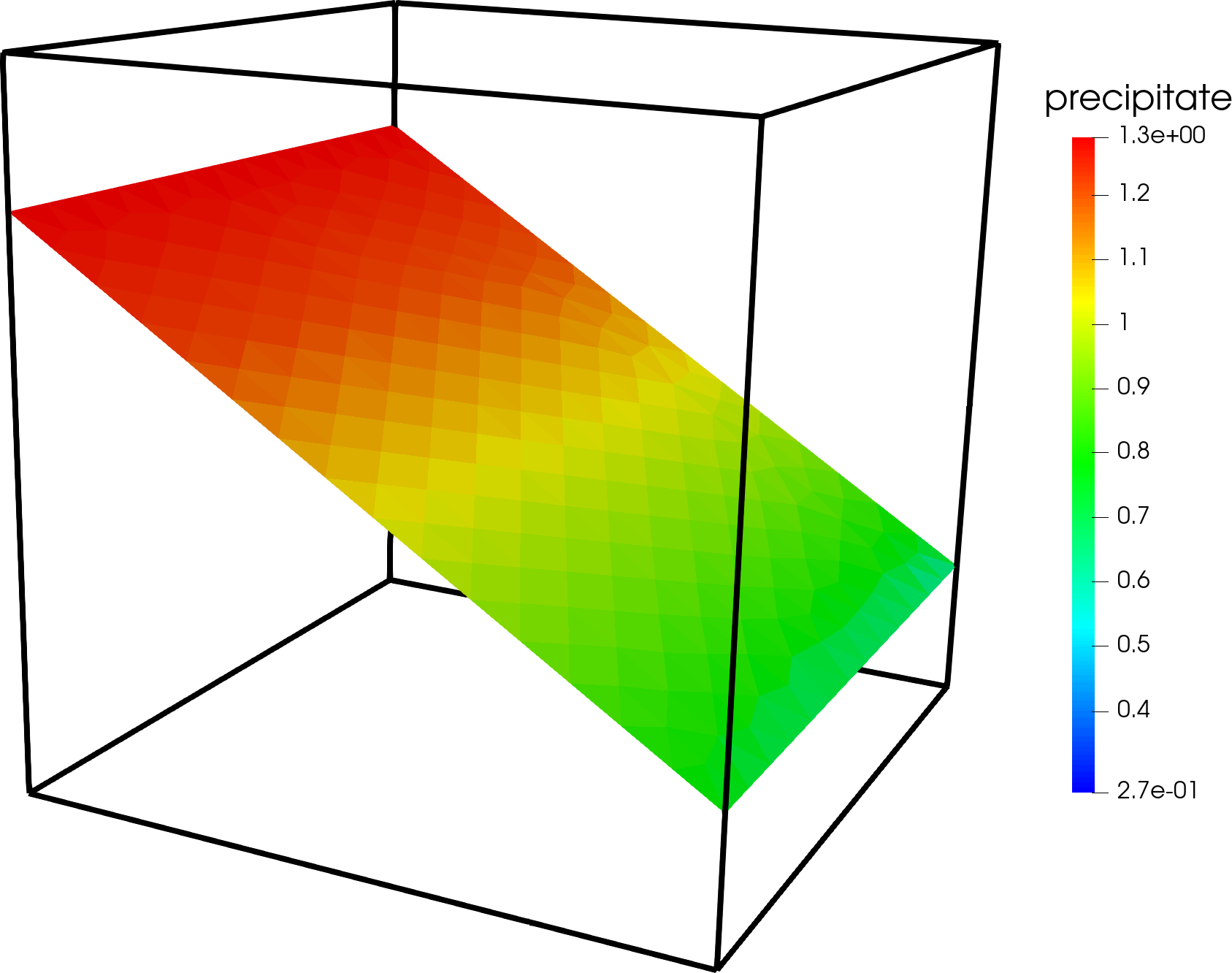
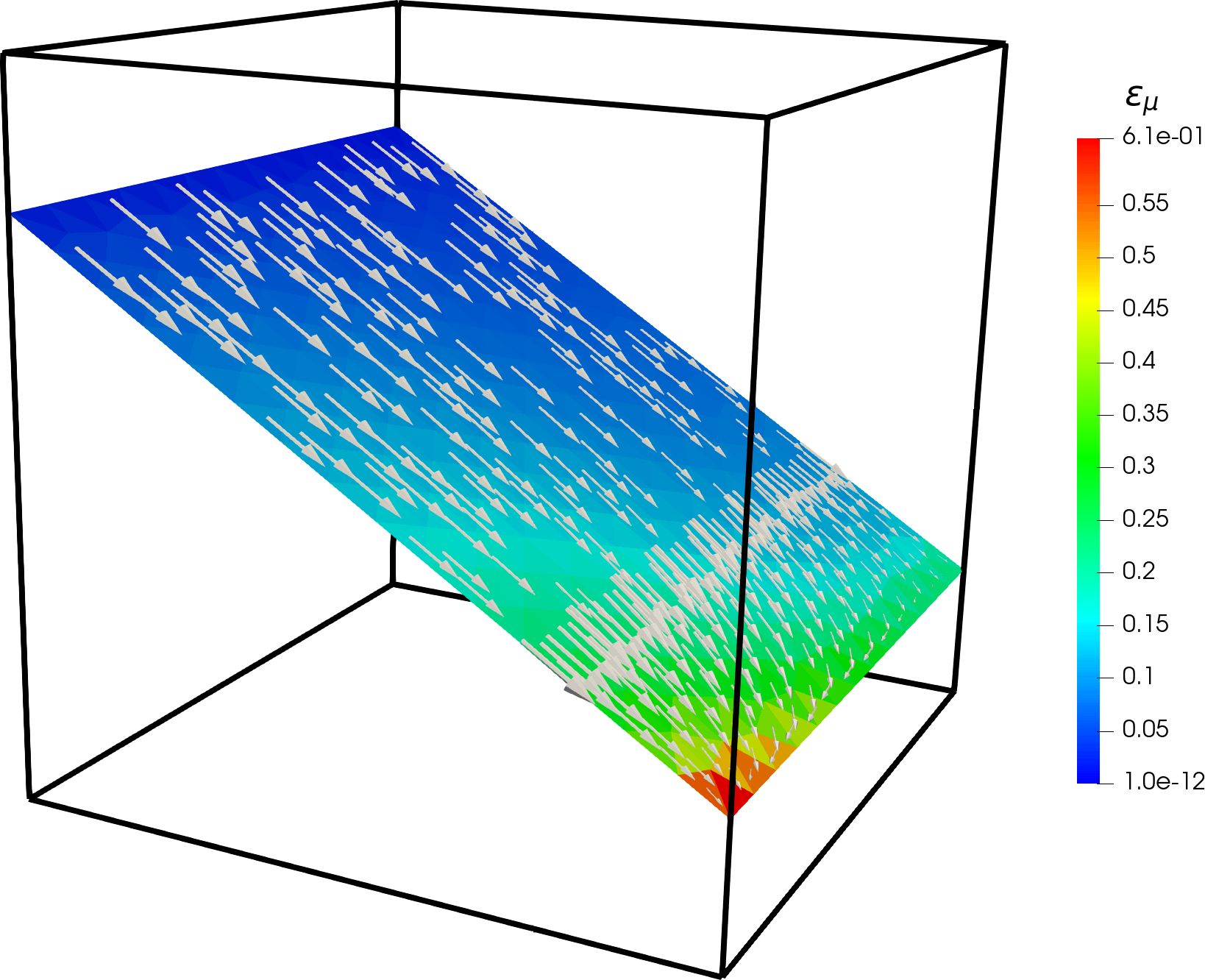
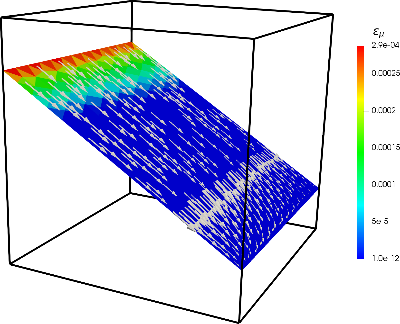
Figure 18: On the top layer precipitate and on the bottom the layer aperture. On the left we observe the portion of the layer on the top (close to the outflow) and on the right the bottom part of the layer. We overlap to the aperture layer the Darcy velocity in the fracture. Note that the last two figures are scaled differently. Solution for the test case in Subsection 4.2.

Considering the size of the computational domain, the values of the layer thickness obtained is in the limit of a reduced model. To be able to capture this small layer around the fracture, and thus use the model in Problem 2, we should refine the grid obtaining a problem that is too computational expensive to solve, even for such simple test case. This test case, with the considered data, shows the importance of the presented multi-layer reduced model, which can be considered an attractive alternative.

5 Conclusion

In this work we have introduced a mathematical model that is able to simulate in an accurate, yet affordable way simple reactive transport flow problems in the presence of a fracture. In particular, when the reaction rate is high enough compared to transport, we observe that a narrow region, denoted as reactive layer, forms just around the fracture: here the porous medium has different physical properties from the surrounding porous matrix due to mineral precipitation or dissolution. These changes in porosity and permeability might substantially alter the flow field, resulting in a fully coupled and non-linear mathematical model. Moreover, in this layer we expect steep gradients of the variables, in particular the solute and precipitate. For large Damköhler numbers, as proven by numerical simulations and experimental observations, these reactive layers can be extremely thin, to the point that it is difficult to capture their geometry and solution dynamics with a refined computational grid. For this reason in this work we have proposed and tested a reduced model where not only the fractures, but the reactive layers as well are represented as co-dimension 1 objects coupled with the porous matrix, and among themselves. We have derived, under suitable assumptions, a model for the evolution in time of the layer thickness which provided reliable results compared to a very refined numerical simulation of the corresponding equi-dimensional model. The model has been derived and tested for a simple linear reaction rate model and, at the steady state only, for a more complex reaction rate that accounts for equilibrium solubility and supersaturation. By increasing further the complexity of the reaction rate we expect that the model for the layer evolution might become more involved and will require a numerical approximated solution (as opposed to a closed form expression) to estimate, at each point and each time step, the layer thickness: this will be part of a future study. In the numerical study we have also shown a three-dimensional model where the proposed approach might be even more attractive to substantially lighten the computational burden associated with mesh refinement.

Conflict of interest

There are no conflict of interest.

References

- [1] Joubine Aghili, Konstantin Brenner, Julian Hennicker, Roland Masson, and Laurent Trenty. Two-phase discrete fracture matrix models with linear and nonlinear transmission conditions. GEM-International Journal on Geomathematics, 10(1):1, 2019.
- [2] Abramo Agosti, Luca Formaggia, and Anna Scotti. Analysis of a model for precipitation and dissolution coupled with a darcy flux. Journal of Mathematical Analysis and Applications, 431(2):752–781, 2015.
- [3] Abramo Agosti, Bianca Giovanardi, Luca Formaggia, and Anna Scotti. A numerical procedure for geochemical compaction in the presence of discontinuous reactions. Advances in Water Resources, 94:332 – 344, 2016.
- [4] Paola F. Antonietti, Chiara Facciolà, Alessandro Russo, and Marco Verani. Discontinuous Galerkin approximation of flows in fractured porous media on polytopic grids. SIAM Journal on Scientific Computing, 41(1):A109–A138, 2019.
- [5] Paola Francesca Antonietti, Luca Formaggia, Anna Scotti, Marco Verani, and Nicola Verzotti. Mimetic finite difference approximation of flows in fractured porous media. ESAIM: M2AN, 50(3):809–832, 2016.
- [6] Jacob Bear and A.H.-D. Cheng. Modeling Groundwater Flow and Contaminant Transport. Springer, 2010.
- [7] Inga Berre, Wietse M. Boon, Bernd Flemisch, Alessio Fumagalli, Dennis Gläser, Eirik Keilegavlen, Anna Scotti, Ivar Stefansson, Alexandru Tatomir, Konstantin Brenner, Samuel Burbulla, Philippe Devloo, Omar Duran, Marco Favino, Julian Hennicker, I-Hsien Lee, Konstantin Lipnikov, Roland Masson, Klaus Mosthaf, Maria Giuseppina Chiara Nestola, Chuen-Fa Ni, Kirill Nikitin, Philipp Schädle, Daniil Svyatskiy, Ruslan Yanbarisov, and Patrick Zulian. Verification benchmarks for single-phase flow in three-dimensional fractured porous media. Advances in Water Resources, 2020. Accepted. Available at arXiv:2002.07005 [math.NA].
- [8] Daniele Boffi, Franco Brezzi, and Michel Fortin. Mixed Finite Element Methods and Applications. Springer Series in Computational Mathematics. Springer Berlin Heidelberg, 2013.
- [9] Wietse M. Boon, Jan M. Nordbotten, and Ivan Yotov. Robust discretization of flow in fractured porous media. SIAM Journal on Numerical Analysis, 56(4):2203–2233, 2018.
- [10] Wietse M. Boon, Jan Martin Nordbotten, and Jon Eivind Vatne. Functional analysis and exterior calculus on mixed-dimensional geometries. Annali Matematica Pura ed Applicata, 2020. In press.
- [11] Bouillard, Nicolas, Eymard, Robert, Herbin, Raphaele, and Montarnal, Philippe. Diffusion with dissolution and precipitation in a porous medium: Mathematical analysis and numerical approximation of a simplified model. ESAIM: M2AN, 41(6):975–1000, 2007.
- [12] Konstantin Brenner, Julian Hennicker, Roland Masson, and Pierre Samier. Hybrid-dimensional modelling of two-phase flow through fractured porous media with enhanced matrix fracture transmission conditions. Journal of Computational Physics, 357:100–124, 2018.
- [13] Kostantin Brenner, Mayya Groza, C. Guichard, and Roland Masson. Vertex approximate gradient scheme for hybrid dimensional two-phase darcy flows in fractured porous media. ESAIM: Mathematical Modelling and Numerical Analysis, 49(2):303–330, 2015.
- [14] Carina Bringedal, Lars von Wolff, and Iuliu Sorin Pop. Phase field modeling of precipitation and dissolution processes in porous media: Upscaling and numerical experiments. Multiscale Modeling & Simulation, 18(2):1076–1112, 2020.
- [15] Florent Chave, Daniele A. Di Pietro, and Luca Formaggia. A hybrid high-order method for darcy flows in fractured porous media. SIAM Journal on Scientific Computing, 40(2):A1063–A1094, 2018.
- [16] Isabelle Faille, Alessio Fumagalli, Jérôme Jaffré, and Jean Elisabeth Roberts. Model reduction and discretization using hybrid finite volumes of flow in porous media containing faults. Computational Geosciences, 20(2):317–339, 2016.
- [17] Bernd Flemisch, Inga Berre, Wietse Boon, Alessio Fumagalli, Nicolas Schwenck, Anna Scotti, Ivar Stefansson, and Alexandru Tatomir. Benchmarks for single-phase flow in fractured porous media. Advances in Water Resources, 111:239–258, Januray 2018.
- [18] Bernd Flemisch and Helmig Rainer. Numerical investigation of a mimetic finite difference method. In Raphael Eymard and Jean-Marc Hèrard, editors, Finite Volumes for Complex Applications V - Problems and Perspectives, pages 815–824. Wiley - VCH, 2008.
- [19] Luca Formaggia, Alessio Fumagalli, Anna Scotti, and Paolo Ruffo. A reduced model for Darcy’s problem in networks of fractures. ESAIM: Mathematical Modelling and Numerical Analysis, 48:1089–1116, 7 2014.
- [20] Luca Formaggia, Anna Scotti, and Federica Sottocasa. Analysis of a mimetic finite difference approximation of flows in fractured porous media. ESAIM Math. Model. Numer. Anal., 52(2):595–630, 2018.
- [21] Alessio Fumagalli and Isabelle Faille. A double-layer reduced model for fault flow on slipping domains with hybrid finite volume scheme. SIAM Journal on Scientific Computing, 77:1–26, June 2018.
- [22] Alessio Fumagalli, Eirik Keilegavlen, and Stefano Scialò. Conforming, non-conforming and non-matching discretization couplings in discrete fracture network simulations. Journal of Computational Physics, 376:694–712, 2019.
- [23] Alessio Fumagalli, Luca Pasquale, Stefano Zonca, and Stefano Micheletti. An upscaling procedure for fractured reservoirs with embedded grids. Water Resources Research, 52(8):6506–6525, 2016.
- [24] Alessio Fumagalli and Anna Scotti. A numerical method for two-phase flow in fractured porous media with non-matching grids. Advances in Water Resources, 62, Part C(0):454–464, 2013. Computational Methods in Geologic CO2 Sequestration.
- [25] Alessio Fumagalli and Anna Scotti. A mathematical model for thermal single-phase flow and reactive transport in fractured porous media. Technical report, arXiv:2005.09437 [math.NA], 2020.
- [26] Alessio Fumagalli and Anna Scotti. A multi-layer reduced model for flow in porous media with a fault and surrounding damage zones. Computational Geosciences, 24(3):1347–1360, 2020.
- [27] Alessio Fumagalli and Anna Scotti. Reactive flow in fractured porous media. Technical Report arXiv:2001.05275 [math.NA], arXiv, 2020.
- [28] Bianca Giovanardi, Anna Scotti, Luca Formaggia, and Paolo Ruffo. A general framework for the simulation of geochemical compaction. Computational Geosciences, 19(5):1027–1046, Oct 2015.
- [29] Eirik Keilegavlen, Runar Berge, Alessio Fumagalli, Michele Starnoni, Ivar Stefansson, Jhabriel Varela, and Inga Berre. Porepy: An open-source software for simulation of multiphysics processes in fractured porous media. Computational Geosciences, 2020.
- [30] Peter Knabner, C.J. van Duijn, and S. Hengst. An analysis of crystal dissolution fronts in flows through porous media. part 1: Compatible boundary conditions. Advances in Water Resources, 18(3):171–185, 1995.
- [31] T.V. Lopes, A.C. Rocha, Murad M.A., Garcia E.L.M., Pereira1 P.A., and Cazarin C.L. A new computational model for flow in karst-carbonates containing solution-collapse breccias. Computational Geosciences, 24:61–87, 2020.
- [32] Vincent Martin, Jérôme Jaffré, and Jean Elisabeth Roberts. Modeling Fractures and Barriers as Interfaces for Flow in Porous Media. SIAM J. Sci. Comput., 26(5):1667–1691, 2005.
- [33] Jan Martin Nordbotten, Wietse Boon, Alessio Fumagalli, and Eirik Keilegavlen. Unified approach to discretization of flow in fractured porous media. Computational Geosciences, 23(2):225–237, 2019.
- [34] Iuliu Sorin Pop, Jeroen Bogers, and Kundan Kumar. Analysis and upscaling of a reactive transport model in fractured porous media with nonlinear transmission condition. Vietnam Journal of Mathematics, 45(1):77–102, Mar 2017.
- [35] Florin Adrian Radu, Iuliu Sorin Pop, and Sabine Attinger. Analysis of an Euler implicit - mixed finite element scheme for reactive solute transport in porous media. Numer. Methods Part. Differ. Equat., 26:320–344, 2010.
- [36] Pierre-Arnaud Raviart and Jean-Marie Thomas. A mixed finite element method for second order elliptic problems. Lecture Notes in Mathematics, 606:292–315, 1977.
- [37] Jean E. Roberts and Jean-Marie Thomas. Mixed and hybrid methods. In Handbook of numerical analysis, Vol. II, Handb. Numer. Anal., II, pages 523–639. North-Holland, Amsterdam, 1991.
- [38] Nicolas Schwenck, Bernd Flemisch, Rainer Helmig, and BarbaraI. Wohlmuth. Dimensionally reduced flow models in fractured porous media: crossings and boundaries. Computational Geosciences, 19(6):1219–1230, 2015.
- [39] Ivar Stefansson, Inga Berre, and Eirik Keilegavlen. Finite-volume discretisations for flow in fractured porous media. Transport in Porous Media, 124(2):439–462, 2018.
- [40] Matei Tene, Sebastian B. M. Bosma, Mohammed Saad Al Kobaisi, and Hadi Hajibeygi. Projection-based embedded discrete fracture model (pEDFM). Advances in Water Resources, 105:205 – 216, 2017.
- [41] Tycho L. van Noorden. Crystal precipitation and dissolution in a porous medium: Effective equations and numerical experiments. Multiscale Modeling & Simulation, 7(3):1220–1236, 2009.