Evolution of three-dimensional coherent structures in Hall magnetohydrodynamics

Abstract

The work extends the computational model EULAG-MHD to include Hall magnetohydrodynamics (HMHD)—important to explore physical systems undergoing fast magnetic reconnection at the order of the ion inertial length scale. Examples include solar transients along with reconnections in magnetosphere, magnetotail and laboratory plasmas. The paper documents the results of two distinct sets of implicit large-eddy simulations in the presence and absence of the Hall forcing term, initiated with an unidirectional sinusoidal magnetic field. The HMHD simulation while benchmarking the code also emphasizes the complexity of three dimensional (3D) evolution over its two dimensional (2D) counterpart. The magnetic reconnections onset significantly earlier in HMHD. Importantly, the magnetic field generated by the Hall term breaks any inherent symmetry, ultimately making the evolution 3D. The resulting 3D reconnections develop magnetic flux ropes and magnetic flux tubes. Projected on the reconnection plane, the ropes and tubes appear as magnetic islands, which later break into secondary islands, and finally coalesce to generate an X-type neutral point. These findings are in agreement with the theory and contemporary simulations of HMHD, and thus verify our extension of the EULAG-MHD model. The second set explores the influence of the Hall forcing on generation and ascend of a magnetic flux rope from sheared magnetic arcades—a novel scenario instructive in understanding the coronal transients. The rope evolves through intermediate complex structures, ultimately breaking locally because of reconnections. Interestingly, the breakage occurs earlier in the presence of the Hall term, signifying faster dynamics leading to magnetic topology favorable for reconnections.

1 Introduction

Magnetofluids characterized by large Lundquist numbers $S=LV_{A}/\eta$ ($L\equiv$ length scale of the the magnetic field ${\bf{B}}$ variability, $V_{A}\equiv$ Alfvén speed, and $\eta\equiv$ magnetic diffusivity) satisfy Alfvén’s flux-freezing theorem on magnetic field lines (MFLs) being tied to fluid parcels (Alfvén, 1942). The astrophysical plasmas are of particular interest, because their inherently large $L$ implies large $S$ and the flux freezing. For example, the solar corona with global $L\approx 10^{6}~{}{\rm m}$, $V_{A}\approx 10^{6}~{}{\rm m}~{}{\rm s}^{-1}$, $B\approx 10~{}{\rm G}$ and $\eta\approx 1~{}{\rm m}^{2}~{}{\rm s}^{-1}$ (calculated using Spitzer resistivity) has a $S\approx 10^{12}$ (Aschwanden, 2005). Nevertheless the coronal plasma also exhibits diffusive behavior. For example, the solar transients—such as flares, coronal mass ejections, and coronal jets—are all manifestations of magnetic reconnections (MRs) that in turn form a diffusive phenomenon, where the magnetic energy gets converted into heat and kinetic energy of plasma flow, accompanied with a rearrangement of MFLs (Choudhuri, 1998). The onset of MRs is due to the generation of small scales in consequence of large scale dynamics, eventually leading to locally reduced characteristic length scale of the magnetic field variability and thereby resulting in intermittently diffusive plasmas. The small scales can owe their origin to the presence of magnetic nulls; i.e., locations where the ${\bf{B}}=0$ (Priest, 2014; Nayak et al., 2020). Alternatively, and more relevant to this paper, this can be due to the presence of current sheets (CSs); i.e., the ribbons of intense current, across which ${\bf{B}}$ has a sharp gradient (Parker, 1994; Kumar & Bhattacharyya, 2011). Spontaneous development of CSs is predicted by the Parker’s magnetostatic theorem that implies the inevitability of CSs in an equilibrium magnetofluid with perfect electrical conductivity. This inevitability in turn is due to the general failure of a smooth magnetic field to simultaneously preserve the local force balance and the global magnetic topology (Parker, 1994).

To elucidate this seminal theorem, we follow the arguments in Kumar & Bhattacharyya (2011). Let us perceive a series of contiguous fluid parcels with their frozen-in MFLs. We further assume the fluid to be incompressible. The magnetic field is everywhere continuous. If the two ends of the series are pushed toward each other, because of incompressibility the interstitial parcels will be squeezed out. Terminally, the end parcels of the series will approach each other and their MFLs being non-parallel (in general)—will create a CS. Notably, for an ideal magnetofluid having infinite electrical conductivity the creation of the CS is the terminal state, but in the presence of a small magnetic diffusivity the MFLs will ultimately reconnect. The reconnected MFLs are subsequently pushed away from the reconnection region by the outflow, and as they come out of the CS, the MFLs once again get frozen to the fluid. Afterward, these frozen MFLs can push another flux system and repeat the whole process of reconnection. This switch between the large and the small scales with their inherent coupling is fundamentally interesting and has the potential to drive a myriad of MR driven phenomena observed in the solar atmosphere.

An example of this scenario is numerically demonstrated by Kumar et al. (2016) using MHD simulations. Their simulations describe the activation of a magnetic flux rope (MFR) by an interplay between the two aforementioned scales. Notably the large scale is relatively independent of the particular system under consideration but identifying the small or the diffusion scale depends on the specific physical system involved. For instance, observations suggests the average MR time for solar flares to be $10^{2}-10^{3}$ s; the impulsive rise time (Priest & Forbes, 2000). Presuming the relation $L\equiv\sqrt{\tau_{d}\eta}$ holding well and the magnetic diffusion time scale $\tau_{d}\approx 10^{3}$ s, the $L$ that initiates the MR turns out to be $\approx 32$ m. The local Lundquist number then gets reduced to $S\approx 3.2\times 10^{7}$. As a consequence, an ion inertial scale $\delta_{i}\approx 2.25$ m in the solar corona (Priest & Forbes, 2000) suggests that the order of the dissipation term, $1/S\approx 10^{-7}$, is much smaller than the order of the Hall term, $\delta_{i}/L\approx 10^{-2}$, in an appropriate dimensionless induction equation (Westerberg & Åkerstedt, 2007)

$$\frac{{\partial\bf{B}}}{\partial t}=\nabla\times\left({\bf{v}}\times{\bf{B}}\right)-\frac{1}{S}\nabla\times{\bf{J}}-\frac{\delta_{i}}{L}\nabla\times\left({\bf{J}}\times{\bf{B}}\right)~{},$$ (1)

where ${\bf{J}}(=\nabla\times{\bf{B}})$ and ${\bf{v}}$ are the volume current density and the plasma flow velocity, respectively. The disparity in the magnitude orders of the dissipation and the Hall forcing suggests that if the dissipation is important, then so is the Hall magnetohydrodynamics (HMHD). It also indicates that HMHD can be crucial for coronal transients—MRs being their underlying reason. By the same token, HMHD is also important in other systems like Earth’s magnetosphere, typically at the magnetopause and the magnetotail where CSs exist (Mozer et al., 2002).

In the HMHD, the ion and electron motions decouple (Sonnerup, 1979), and the MFLs are frozen in the electron fluid instead of the ion fluid. Additionally, straightforward mathematical manipulations show that the Hall term in the induction equation does not affect the dissipation rate of magnetic energy and magnetic helicity (Priest & Forbes, 2000). Given the unique properties of HMHD, we expect it to reveal subtle changes in MFLs evolution familiar from the standard MHD (Kumar et al., 2016; Nayak et al., 2019, 2020), and refine the dynamics leading to magnetic reconnections. To further explore HMHD specifically contextual to the solar physics, we have extended the EULAG-MHD model (Smolarkiewicz & Charbonneau, 2013; Charbonneau & Smolarkiewicz, 2013) by including the Hall forcing and document here the results pertaining to two distinct sets of large-eddy simulations. The first set focuses on benchmarking the numerical model by verifying the HMHD physics in three spatial dimensions. The simulations highlight the complexity in reconnection-assisted formation of coherent magnetic structures, hitherto less explored in the contemporary research. The second set, simulates, for the first time to our knowledge, the formation and evolution of a magnetic flux rope (MFR) under the influence of the Hall forcing—initiated from sheared bipolar magnetic loops relevant to the solar corona.

Related to our simulations, Mozer et al. (2002) using 2D geometry have shown that the Hall forcing causes the electrons residing on the reconnection plane containing the MFLs to flow into and out of the reconnection region, generating the in-plane current. The in-plane current, in turn, develops a magnetic field having component out of the reconnection plane. This out-of-plane magnetic field, or the Hall magnetic field, has quadrupole structure. The asymmetric propagation of the reconnection plane, because of a “reconnection wave” has been shown by Huba & Rudakov (2002) in a simulation of 3D MR in the Hall limit, where curved out-of-plane MFLs along with the density gradient play a crucial role.

The remainder of the paper is organized as follows. Section 2 outlines the numerical model. Section 3 benchmarks the code using 3D simulations and, subsequently presents a novel numerical experiment that compares activation of a solar-like MFR under standard MHD and HMHD formulations. Section 4 summarizes the key findings of this work.

2 The numerical model

A numerical simulation consistent with physics of solar corona must accurately preserve the flux-freezing by minimizing numerical dissipation and dispersion errors away from the reconnection regions characterized by steep gradients of the magnetic field (Bhattacharyya et al., 2010). Such minimization is a signature of a class of inherently nonlinear high-resolution transport methods that preserve field extrema along flow trajectories, while ensuring higher-order accuracy away from steep gradients in advected fields. Consequently, we incorporate the Hall forcing in the established high-resolution EULAG-MHD model (Smolarkiewicz & Charbonneau, 2013; Charbonneau & Smolarkiewicz, 2013), a specialized version of the general-purpose hydrodynamic model EULAG predominantly used in atmospheric and climate research (Prusa et al., 2008). Central to the EULAG is the spatio-temporally second-order-accurate nonoscillatory forward-in-time (NFT) advection scheme MPDATA, a.k.a Multidimensional Positive Definite Advection Transport Algorithm, (Smolarkiewicz, 2006). A feature unique to MPDATA and important in our calculations is its widely-documented dissipative property that mimics the action of explicit subgrid-scale turbulence models, wherever the concerned advective field is under-resolved—the property referred to as implicit large eddy simulations (ILES) (Grinstein et al., 2007). The resulting MRs remove the under-resolved scales and restore the flux-freezing. These MRs being intermittent and local, successfully mimic physical MRs. The ILES property of MPDATA have proven instrumental in a series of advanced numerical studies across a range of scales and physical scenarios, including studies related to the coronal heating along with data-constrained simulations of solar flares and coronal jets (Bhattacharyya et al., 2010; Kumar & Bhattacharyya, 2011; Kumar et al., 2015, 2017; Prasad et al., 2017; Prasad et al., 2018; Nayak et al., 2019, 2020). The simulations reported in this paper also benefit from ILES property of MPDATA.

Here, the numerically integrated HMHD equations assume a perfectly conducting, incompressible magnetofluid. Using a conservative flux-form and dyadic notation, they are compactly written (assuming cgs units) as

$$\frac{\partial{\bf v}}{\partial t}+\nabla\cdot{\bf v}{\bf v} = -\nabla\phi+\frac{1}{4\pi\rho_{0}}\nabla\cdot{\bf B}{\bf B}+\mu_{0}\nabla^{2}{\bf v}~{},$$ (2)

$$\frac{\partial{\bf B}}{\partial t}+\nabla\cdot{\bf v}{\bf B} = \nabla\cdot{\bf B}{\bf v}-\frac{d_{0}}{4\pi}\left(\nabla\times\nabla\cdot{\bf B}{\bf B}\right)-\nabla\phi^{*}~{},$$ (3)

$$\nabla\cdot{\bf v} = 0~{},$$ (4)

$$\nabla\cdot{\bf B} = 0~{},$$ (5)

where $\rho_{0}$ and $\mu_{0}$ denote, respectively, constant density and kinematic viscosity, $\phi=\left(p+\textbf{B}^{2}/8\pi\right)/\rho_{0}$ is the density normalized total pressure, and $d_{0}=\sqrt{4\pi}\delta_{i}/\rho_{0}$; the $-\nabla\phi^{*}$ term on the right-hand-side (rhs) of (3) will be explained shortly.

To highlight the numerics of EULAG-MHD and its extension to HMHD, the prognostic PDEs (2) and (3) are further symbolized as a single equation

$$\frac{\partial{\bf\Psi}}{\partial t}+\nabla\cdot{\bf v\Psi}={\bf R}{\bf\Psi}~{},$$ (6)

where ${\bf\Psi}=\{v_{x},v_{y},v_{z},B_{x},B_{y},B_{z}\}^{T}$ is the vector of prognosed variables, and ${\bf R}({\bf\Psi})$ is the vector of their associated rhs forcings. The principal second-order-accurate NFT Eulerian algorithm for (6) can be written compactly as

$${\bf\Psi}_{\bf i}^{n}={\mathcal{A}}_{\bf i}\left({\bf{{\Psi}}}^{n-1}+\delta_{h}t\,{\bf R}^{n-1},{\bf v}^{n-1/2}\right)+\delta_{h}t\,{\bf R}({\bf\Psi})|^{n}_{\bf i}~{}\equiv~{}\widehat{\bf\Psi}_{\bf i}+\delta_{h}t\,{\bf R}({\bf\Psi})|^{n}_{\bf i}~{},$$ (7)

where $n$, ${\bf i}$ refer to $(t^{n},{\bf x}_{\bf i})$ locations on a regular collocated grid, $\delta t$ marks the time step with $\delta_{h}t=0.5\delta t$, and ${\cal{A}}$ denotes the MPDATA advection operator, solely dependent on the preceding, $t^{n-1}=t^{n}-\delta t$, values of ${\bf\Psi}$ as well as a first-order estimate of the solenoidal velocity at $t^{n}-\delta_{h}t$ extrapolated from the earlier values.

The principal algorithm (7) is implicit for all prognosed variables and diagnosed potentials $\phi$ and $\phi^{*}$ that enter (2) and (3), respectively. While $\phi$ is a physical variable, $\phi^{*}$ is a numerical facilitator enabling restoration of (5)—viz. divergence cleaning—eventually polluted with truncation errors. Because of its nonlinearity, the rhs ${\bf{R}}$ of (7) is viewed as a combination of a linear term ${\bf{L}}{\bf\Psi}$ (with ${\bf L}$ denoting a known linear operator), a nonlinear term ${\bf N}({\bf\Psi})$, and the potential term $-\nabla{\bf{\Phi}}$ with ${\bf{\Phi}}\equiv(\phi,~{}\phi,~{}\phi,~{}\phi^{*},~{}\phi^{*},~{}\phi^{*})^{T}$. The resulting form of (7) is realized iteratively with the nonlinear part of the rhs forcing lagged behind,

$${\mathbf{\Psi}}^{n,\nu}_{\bf i}={\widehat{\mathbf{\Psi}}}_{\bf i}+\delta_{h}t\ {\mathbf{L}}{\mathbf{\Psi}}\big{|}^{n,\nu}_{\bf i}+\delta_{h}t\ {\mathbf{N}}({\mathbf{\Psi}})\big{|}^{n,\nu-1}_{\bf i}-\delta_{h}t\ \nabla{\mathbf{\Phi}}\big{|}^{n,\nu}_{\bf i}~{},$$ (8)

where $\nu=1,..,m$ numbers the iterations. The algorithm in (8) is still implicit with respect to ${\bf{\Psi}}^{n,\nu}_{\bf i}$ and ${\bf{\Phi}}^{n,\nu}_{\bf i}$, yet straightforward algebraic manipulations lead to the closed-form expression

$${\mathbf{\Psi}}^{n,\nu}_{\bf i}=\left[{\mathbf{I}}-\delta_{h}t{\mathbf{L}}\right]^{-1}\left({\widehat{\widehat{\mathbf{\Psi}}}}-\delta_{h}t{\nabla}{\mathbf{\Phi}}^{n,\nu}\right)\Big{|}_{\bf i}~{},$$ (9)

where ${\widehat{\widehat{\mathbf{\Psi}}}}\equiv{\widehat{\mathbf{\Psi}}}+\delta_{h}t{\mathbf{N}}{\mathbf{\Psi}}\big{|}^{n,\nu-1}$ denotes the modified explicit element of the solution. Taking the divergences of the first and the second three components of (9), produces two elliptic Poisson problems, for $\phi$ and $\phi^{*}$, respectively, as implied by (4) and (5).

The iterative formulation of (7) in (8), outlines the concept of the EULAG-MHD discrete integrals. The actual iterative implementation of (7), detailed in (Smolarkiewicz & Charbonneau, 2013), proceeds in a sequence of steps such that the most current update of a dependent variable is used in the ongoing step, wherever possible. Furthermore, to enhance the efficacy of the scheme, judicious linearization of ${\bf N}({\mathbf{\Psi}})$ is employed, together with a blend of evolutionary and conservative forms of the induction and Lorentz forces. Each outer iteration has two distinct blocks. The focus of the first,“hydrodynamic” block is on integrating the momentum equation, where the magnetic field enters the Lorentz force and is viewed as supplementary. This block ends with the final update of the velocity via the the solution of the elliptic problem for pressure. The second, “magnetic” block uses the current updates of the velocities to integrate the induction equation. It ends with the final update of the magnetic field via the solution of the elliptic problem for the divergence cleaning. Incorporating the Hall forcing into the EULAG-MHD model follows the principles of the outlined standard MHD integrator. Because the Hall term enters (3) as the curl of the Lorentz force, it can be judiciously updated and combined with the standard induction forcing, whenever the Lorentz force and/or the magnetic field are updated. In the current implementation it enters the explicit (lagged) counterpart of the induction force, and is updated after the inversion of the implicit evolutionary form of the induction equation in the “magnetic” block; cf. section 3.2 in (Smolarkiewicz & Charbonneau, 2013) for details.

3 Results

3.1 Benchmarking the 3D HMHD solver

To benchmark the HMHD solver, the initial field is selected as

$$B_{x}=0~{},$$ (12)

$$B_{y}=0~{},$$

$$B_{z}=2.5\sin(x)~{},$$

with $x,y,z\in[-2\pi,2\pi]$, respectively, in each direction of a 3D Cartesian domain. This selection has two merits: first, the magnetic field reverses at $x$=0; and second, the Lorentz force

$$({\bf{J}}\times{\bf{B}})_{x}=-6.25\cos(x)\sin(x)\hskip 2.84544pt~{},$$ (13)

$$({\bf{J}}\times{\bf{B}})_{y}=0~{},$$ (14)

$$({\bf{J}}\times{\bf{B}})_{z}=0~{},$$ (15)

generates a converging flow that onsets MRs. Being different from the traditional initial conditions involving the Harris current sheet or the GEM challenge (Birn et al., 2001), this selection shows the Hall effects are independent of particular initial conditions. We have explored simulations using the traditional initial conditions (not shown) and the outcomes are similar.

The equations (2)-(5) are integrated numerically, as described in the preceding section, for $d_{0}=0,~{}2$. The latter selection of $d_{0}$ optimizes the computation time and a tractable development of magnetic structures for the employed spatio-temporal resolution. The corresponding $\delta_{i}=0.56$ is slightly higher than the spatial stepsize $\delta{\bf{x}}\approx 0.40$ set for the simulation. Consequently, the Hall forcing kicks in near the dissipation scale, thereby directly affecting the overall dynamics only in vicinities of the MR regions. With the large scale $L=4\pi$ of the magnetic field variability, the resulting $\delta_{i}/L\approx 0.04$ is on the order of solar coronal value. The simulations are then expected to capture dynamics of the HMHD and the intermittently diffusive regions of corona-like plasmas, thus shedding light on the evolution of neighboring frozen-in MFLs. Moreover, $1/S<\delta_{i}/L$ as discussed in Introduction. The physical domain is resolved with $32\times 32\times 32$ grid. A coarse resolution is selected for an earlier onset of MRs and to expedite the overall evolution. The kinematic viscosity and mass density are set to $\nu=0.005$ and $\rho_{0}=1$, respectively. All three boundaries are kept open. The initial magnetic field is given by the equations (12-12) and the fluid is evolved from an initially static state having pressure $p=0$. The simulation parameters are listed in Table 1.

Table 1: List of parameters for simulation with sinusoidal initial field

$\rho_{0}$	$d_{0}$	$\delta_{i}$	L	$\frac{\delta_{i}}{L}$	Simulation Box Size	Resolution	$\nu$
1.0	2.0	0.56	$4\pi$	0.04	$(4\pi)^{3}$	$(32)^{3}$	0.005

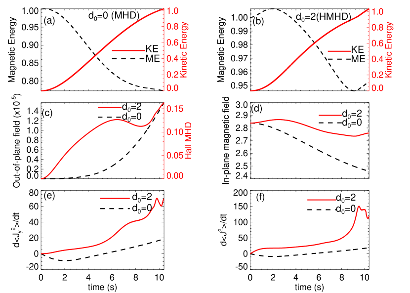
Figure 1: Panels (a) and (b) show the evolution of the magnetic energy (black dashed curve) and kinetic energy (red solid curve) for $d_{0}=0$ (MHD) and $d_{0}=2$ (HMHD) respectively. Panel (c) shows the evolution of out-of-plane magnetic field for $d_{0}=0$ (MHD) with black dashed curve and $d_{0}=2$ (HMHD) with red solid curve respectively. Also in panels (a) to (c), the scales for the solid and the dashed curves are spaced at right and left respectively. Panels (d) to (f) represent in-plane magnetic field, amplitudes of the rate of change of out-of-plane and total current densities for $d_{0}=0$ (black dashed curve) and $d_{0}=2$ (red solid curve) respectively. The variables in panels (a) and (b) are normalized with the initial total energies. All the variables are averaged over the computational domain. Important are the generation of the out-of-plane magnetic field along with sharp changes in time derivatives of the out-of-plane and total volume current densities in HMHD simulations.

The overall evolution is depicted in different panels of Figure 1. The initial Lorentz force, given by equations (13-15), pushes segments of the fluid on either sides of the field reversal layers—toward each other. Consequently, magnetic energy gets converted into kinetic energy of the plasma flow: panels (a) and (b). Panels (c) and (d) show history of grid-averaged magnitude of the the out-of-plane (along $y$) and in-plane ($xz$ plane) magnetic fields. Notably, for $d_{0}=0$ (MHD) the out-of-plane field is negligibly small compared to its value for $d_{0}=2$ (HMHD). Such generation of the out-of-plane magnetic field is inherent to HMHD and is in conformity with the result of another simulation (Ma & Bhattacharjee, 2001). The panels (e) and (f) illustrate the variation of the rate of change of out-of-plane current density and total volume current density. Importantly, in contrast to the $d_{0}=0$ curve, the rate of change of volume current density shows an early bump at $(\approx 7.5$ s) and a well defined peak ($t\approx 9.75$ s) for $d_{0}=2$. Such peaks in the current density are expected in the impulsive phase of solar flares, and they manifest MRs in the presence of the Hall term (Bhattacharjee, 2004).

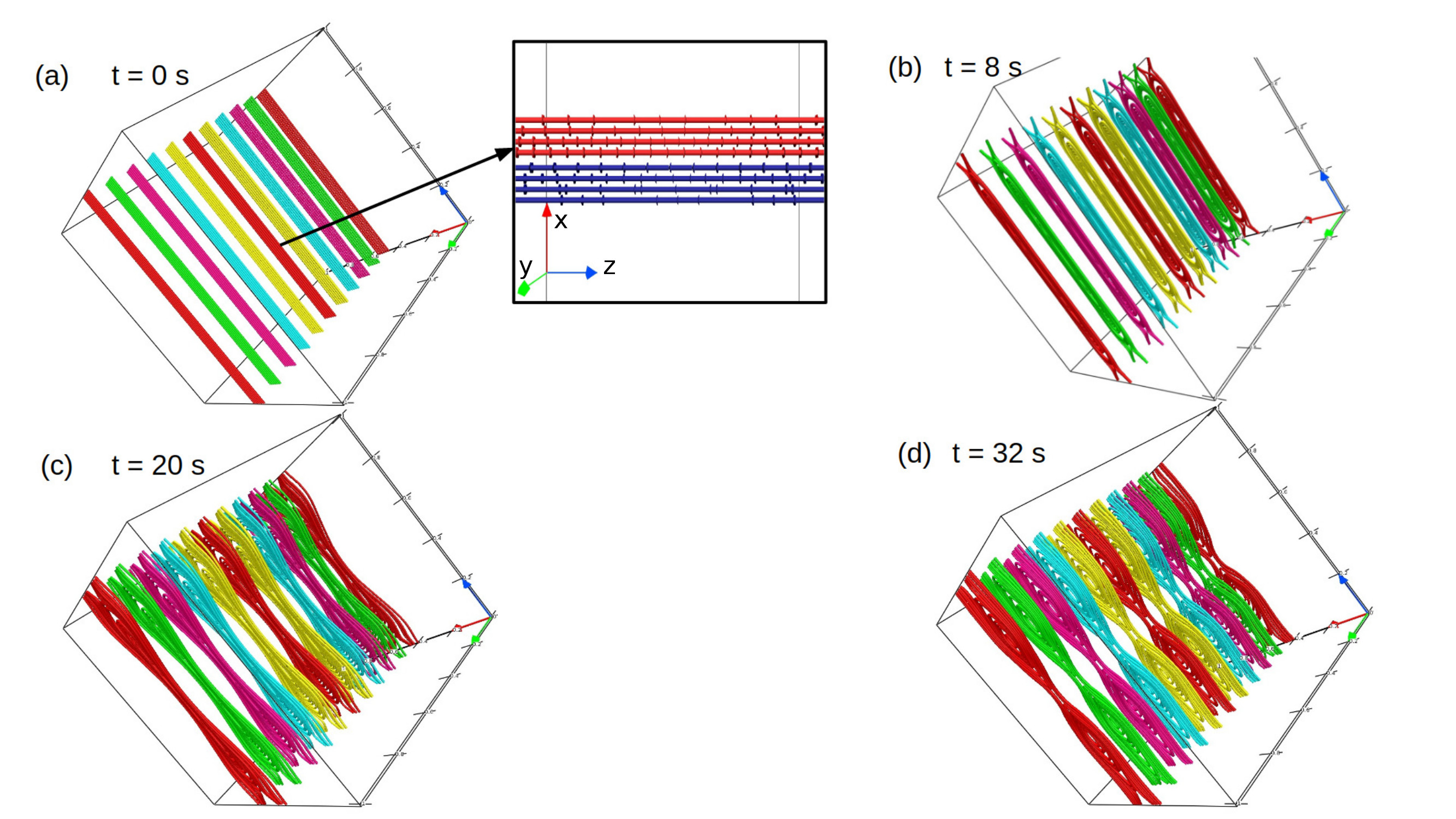
Figure 2: Snapshots of preselected MFLs for the $d_{0}=0$ (MHD) simulation, plotted on equidistant y-constant planes. In all figures (this and hereafter), the red, green and blue arrows represent the x, y and z-axis respectively. The inset in panel (a) highlights the polarity reversal of the initial magnetic field lines. The plots illustrate the formation of a primary flux tube (panel (b)) made by stacking of the depicted MFLs. Notably symmetry is preserved throughout evolution. (An animation of this figure is available.)

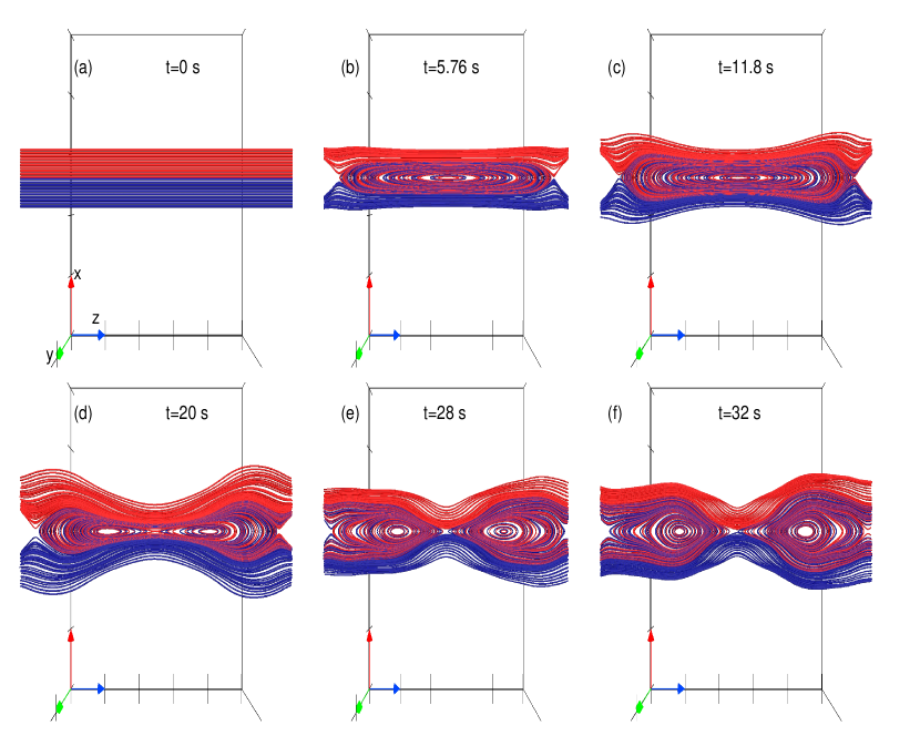
Figure 3: Projection of MFLs depicted in Figure 2 on a $y$ constant plane during their evolution. Notable is the formation of a primary magnetic island having a single O-type neutral point. Subsequently, the primary island breaks into two secondary islands which are separated by an X type neutral point.

Figure 2 plots MFLs tangential to pre-selected planes during different instances of the evolution for $d_{0}=0$. The panel (a) plots the initial MFLs for referencing. The initial Lorentz force pushes anti-parallel MFLs (depicted in the inset) toward each other. Subsequently, X-type neutral points develop near $z=\pm 2\pi$. The consequent MRs generate a complete magnetic island which maintains its identity for a long time. Such islands, stacked on each other along the $y$, generate an extended magnetic flux tube (MFT) at the center, which in its generality is a magnetic flux surface. Further evolution breaks the MFT such that the cross section of the broken tube yields two magnetic islands. The point of contact between the two tear-drop shaped MFLs generates an X-type neutral point. Notably, within the computational time, no field is generated along the $y$ direction and the corresponding symmetry is exactly preserved. In Figure 3 we provide the 2D projection of the MFLs on the $y=0.5$ plane, for later comparison with similar projection for the $d_{0}=2$ case.

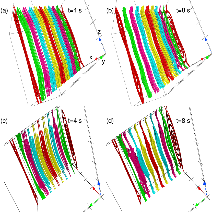
Figure 4: MFL evolution for $d_{0}=2$ (HMHD) case, from two vantage points. The field lines are plotted on planes centered at $x=0.5$ and $x=0.74435$ and equidistant along $y$. Important is the symmetry breaking, cf. MFLs at $y=-2\pi$ and $y=2\pi$ of the panel (b) and (d). The out-of-plane magnetic field is generated throughout the domain. (A combined animation showing MFL evolution for the top and the bottom panels is available.)

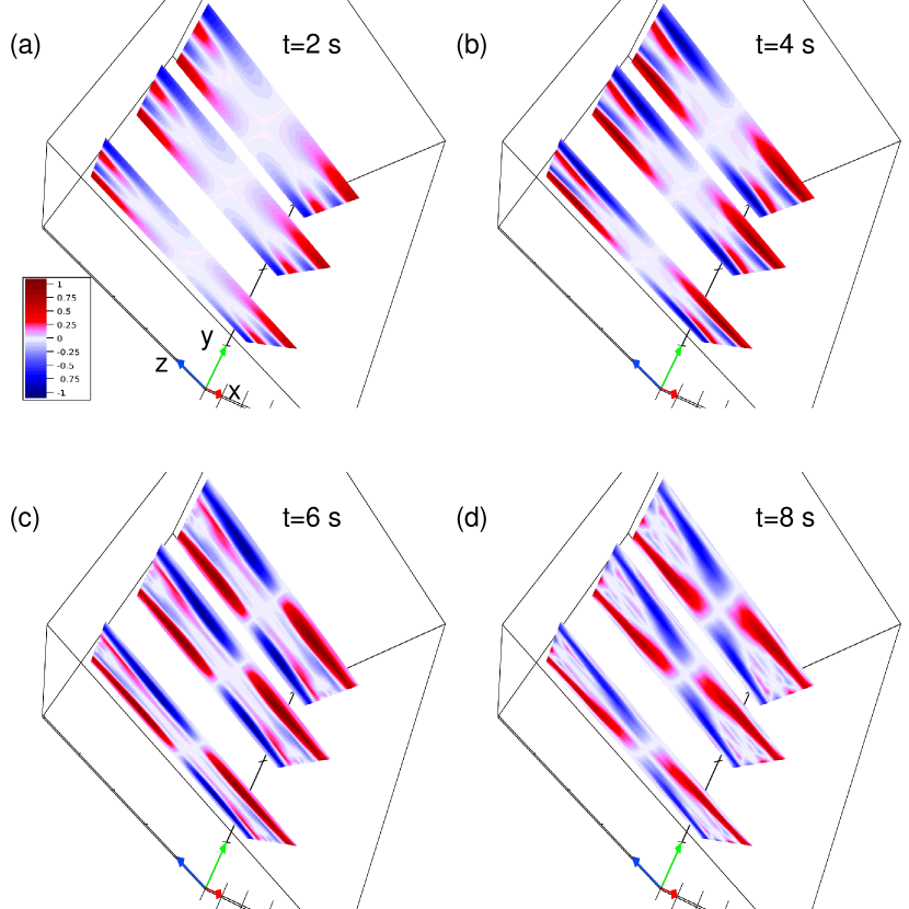
Figure 5: Contour plots of $B_{y}(x,z)$ (out-of-plane component) on y-constant planes for $d_{0}=2$ (HMHD), with time. The plots confirm the quadrupolar nature of the out-of-plane component of the magnetic field.

The panels (a) to (b) and (c) to (d) of Figure 4 show MFL evolution for $d_{0}=2$ from two different vantage points. The MFLs are plotted on different $y$-constant planes centered at $x=0.5$ and $x=0.74435$. The planes are not connected by any field lines at $t=0$. Importantly out-of-plane magnetic field is generated with time in both sets of MFLs (at $x=0.5$ and $x=0.74435$), which connects two adjacent planes (cf. panel (b) of Figures 2 and 4) and breaks the $y$-symmetry that was preserved in the $d_{0}=0$ case — asymmetry in reconnection planes. Consequently the evolved ${\bf{B}}$ is three-dimensional. Also, the out-of-plane component ($B_{y}$) has a quadrupole structure, shown in Figure 5, which is in congruence with observations and models (Mozer et al., 2002).

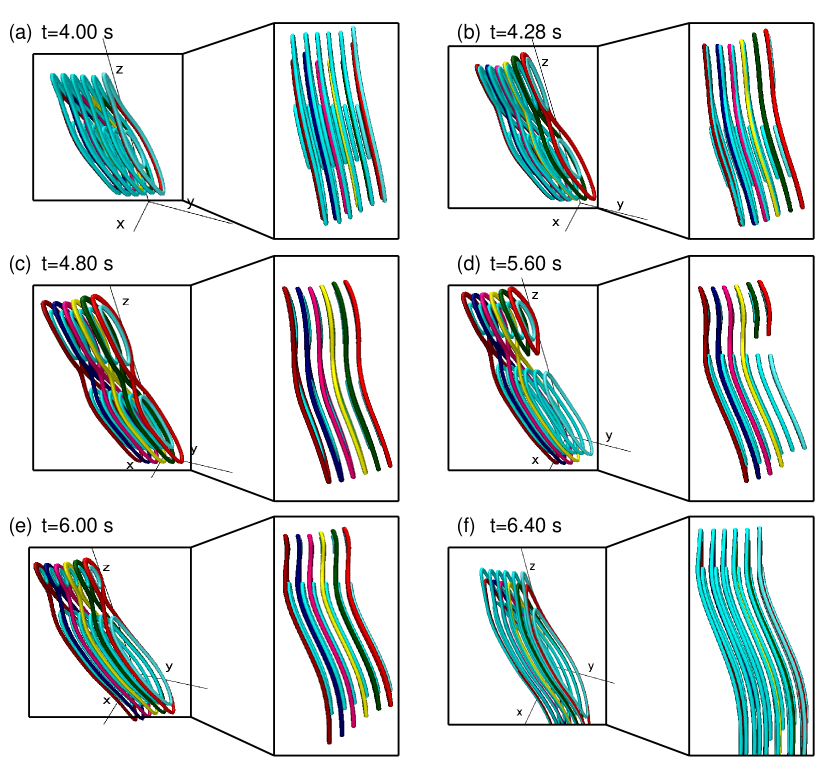
Figure 6: Panels (a) to (f) show the MFL evolution for $d_{0}=2$ (HMHD) case, from two different angles to highlight the generation of two MFTs constituted by disjoint MFLs. The islands look like “figure 8” structure; Panels (b) to (d). The side view of the MFLs are shown in the insets, highlighting their undulated geometry. The three black lines in the background represent the three axes.

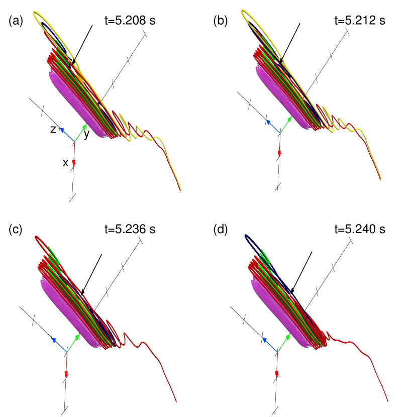
Figure 7: Panels (a) and (b) show the topology of the MFLs for the $d_{0}=2$ (HMHD) evolution, prior and after the internal reconnection of the dark blue colored MFL (marked by the arrow). Panels (c) and (d) depict the topology of MFLs prior and after the internal reconnection of blue and red color MFLs within rope, marked by arrow. (An animation of this figure is available.)

For better clarity the MFLs evolution is further detailed in Figures 6 and 7. In Figure 6 important is the development of two MFTs constituted by disjointly stacked magnetic islands. The islands are undulated and appear much earlier compared to the $d_{0}=0$ case, indicating the faster reconnection. Notable is also the creation of flux ropes where a single helical MFL makes a large number of turns as the out-of-plane field $B_{y}$ develops (Figure 7). In principle, the MFL may ergodically span the MFS, if the “safety factor” $q=rB_{y}/{\mathcal{L}}B_{T}$ is not a rational number (Freidberg, 1982); here $r$ and ${\mathcal{L}}$ are the radius and length of the rope, respectively, and $B_{T}=\sqrt{B_{x}^{2}+B_{y}^{2}}$ . Further evolution breaks the flux rope into secondary ropes by internal MRs—i.e., reconnections between MFLs constituting the rope—shown in panels (a) to (d) of Figure 7, where two oppositely directed sections of the given MFLs reconnect (location marked by arrows in the Figure 7). Since most of the contemporary Hall simulations are in 2D, in Figure 8 we plot the projection of MFLs depicted in Figure 4 on $y=0.5$ plane. The corresponding evolution is visibly similar to the generation of secondary islands (Shi et al., 2019), and their later coalescence as envisioned by Shibata & Tanuma (2001).

To complete the benchmarking, we repeated the numerical experiment described in Huba (2003), where wave propagation in the presence of the Hall forcing is explored. Notably, the EULAG-MHD being incompressible, we only concentrate on the whistler wave. The experimental setup is identical to that in the Huba (2003); the ambient field is given by

$${\bf{B}}=B_{0}\cdot\hat{e_{z}}~{},$$ (16)

whereas the perturbations are

$$\delta B_{x}=\delta B_{0}\sin\left(\frac{2\pi mz}{L_{0}}\right)~{},$$ (17)

$$\delta B_{y}=\delta B_{0}\cos\left(\frac{2\pi mz}{L_{0}}\right)~{},$$ (18)

where $B_{0}=1000$, $\delta B_{0}=10$ and $L_{0}=7\pi$. The mode number is represented by m. The simulations are carried out on a computational domain of size $128\times 128\times 128$ and the dimensionless HMHD equations (discussed shortly) are employed. The analytical and the numerical frequencies obtained for various modes are listed in the Table-2, confirming the simulations to replicate the analytical calculations fairly well.

Table 2: List of parameters for the wave simulation

m	Analytical frequency ($\omega_{A}$)	Numerical frequency ($\omega_{N}$)
2	26.12	27.50
3	132.237	141.88
4	417.92	430.04

3.2 Activation of magnetic flux rope from bipolar magnetic field

Sheared bipolar magnetic field is ubiquitous in solar plasma and plays an important role in the onset of solar transients. In brief, the coronal mass ejection models require magnetic flux ropes (MFRs) to confine plasma. Destabilized from its equilibrium, as the MFR ascends with height—it stretches the overlaying MFLs. The ascend of the rope decreases the magnetic pressure below it which, in turn sucks in more MFLs. These non-parallel MFLs reconnect and the generated outflow further pushes the MFR up. Details about the coronal mass ejection can be found in the review article by (Chen, 2011). Recently, Kumar et al. (2016) numerically simulated the above scenario to explain generation and dynamics of a MFR beginning from initial sets of sheared and twisted MFLs. In the following, we conduct simulations to numerically explore such activations of MFRs in the presence of the Hall term. For this purpose, we employ dimensionless form of the HMHD equations achieved through the following normalizations (Kumar et al., 2016)

$${\bf{B}}\longrightarrow\frac{{\bf{B}}}{B_{0}},\quad{\bf{v}}\longrightarrow\frac{\bf{v}}{v_{A}},\quad L\longrightarrow\frac{L}{L_{0}},\quad t\longrightarrow\frac{t}{\tau_{a}},\quad p\longrightarrow\frac{p}{\rho{v_{a}}^{2}}~{}.$$ (19)

The constant $B_{0}$ is kept arbitrary, whereas $L_{0}$ is fixed to the system size. Further, $v_{A}\equiv B_{0}/\sqrt{4\pi\rho_{0}}$ is the Alfvén speed, where $\rho_{0}$ is a constant mass density. The $\tau_{A}$ and $\tau_{\nu}$ are respectively the Alfvén transit time ($\tau_{A}=L_{0}/v_{A}$) and viscous diffusion time scale ($\tau_{\nu}=L_{0}^{2}/\nu$). The kinematic viscosity is denoted by $\nu$. The normalized equations can be readily visualized by setting $1/(4\pi\rho_{0})=1$ and $\mu_{0}=\tau_{A}/\tau_{\nu}$ in (2), $d_{0}/(4\pi)=\delta_{i}/L$ in (3), while keeping (4) and (5) unchanged. The ratio $\tau_{A}/\tau_{\nu}$ is an effective viscosity of the system which, along with the other forces, influences the magnetofluid evolution.

The simulation is initiated with the magnetic field given in Kumar et al. (2016)

$$B_{x} =k_{z}\sin(k_{x}x)\exp\left(\frac{-k_{z}z}{s_{0}}\right)~{},$$ (20)

$$B_{y} =\sqrt{k_{x}^{2}-k_{z}^{2}}\sin(k_{x}x)\exp\left(\frac{-k_{z}z}{s_{0}}\right)~{},$$ (21)

$$B_{z} =s_{0}k_{x}\cos(k_{x}x)\exp\left(\frac{-k_{z}z}{s_{0}}\right)~{},$$ (22)

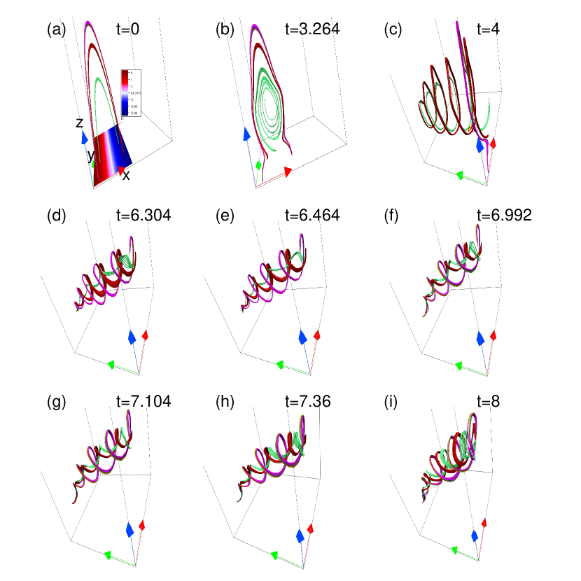
Figure 9: Panel (a) shows the initial bipolar sheared arcade configuration along with polarity inversion line, Panels (b) and (c) show the formation of magnetic flux rope. Panels (d) to (i) represent the further evolution of the magnetic flux rope with a tilted axis (along $y$) of it for $\delta_{i}/L=0$ (MHD) case.

with $k_{x}=1.0$, $k_{z}=0.9$ and $s_{0}=6$. The effective viscosity and mass density are set to $\tau_{A}/\tau_{\nu}=2\times 10^{-5}$ and $\rho_{0}=1$, respectively. The MFLs are depicted in panel (a) of Figure 9 which are sheared bipolar loops having a straight Polarity Inversion Line (PIL) and no field-line twist. For simulations, a physical domain of the extent [$\{0,2\pi\},\{0,2\pi\},\{0,8\pi\}$] is resolved on the computational domain of size $64\times 64\times 128$, making the spatial step sizes $\delta x=\delta y=0.0997,~{}\delta z=0.1979$. The temporal step size is $\delta t=16\times 10^{-4}$. The initial state is assumed to be motionless and open boundary conditions are employed. The simulations are carried out for $\delta_{i}/L_{0}=0$ and $\delta_{i}/L_{0}=0.04$, having a simulated physical time of $7000\tau_{A}\delta t$. The arbitrary $B_{0}$ can be selected such that the Alfvén transit time, $\tau_{A}\in\{1,10\}$ s makes the simulated time, $11.2$ s to $112$ s consistent with the beginning of the impulsive phase of a flare $100$ s to $1000$ s. The simulation parameters for MFR are listed in the Table 3.

Table 3: List of parameters for simulation with bipolar sheared magnetic arcade initial field

$\rho_{0}$	$\delta_{i}$	L	$\frac{\delta_{i}}{L}$	Simulation Box Size	Resolution	Effective Viscosity $\frac{\tau_{A}}{\tau_{\nu}}$
1.0	1.005	$8\pi$	0.04	$2\pi\times 2\pi\times 8\pi$	$64\times 64\times 128$	2$\times$10-5

The evolution onsets as the Lorentz force

$$(\textbf{J}\times\textbf{B})_{x} =\left[-k_{x}(k_{x}^{2}-k_{z}^{2})+k_{x}s_{0}\left(s_{0}k_{x}^{2}-\frac{k_{z}^{2}}{s_{0}}\right)\right]\times\sin^{2}(k_{x}x)\exp\left(-\frac{2k_{z}z}{s_{0}}\right)~{},$$ (23)

$$(\textbf{J}\times\textbf{B})_{z} =\left[\frac{k_{z}}{s_{0}}(k_{x}^{2}-k_{z}^{2})-k_{z}\left(s_{0}k_{x}^{2}-\frac{k_{z}^{2}}{s_{0}}\right)\right]\times\frac{\sin(2k_{x}x)}{2}\exp\left(-\frac{2k_{z}z}{s_{0}}\right)~{},$$ (24)

pushes oppositely directed segments of MFLs toward each other, generating the neck at $t=3.264$, panel (b) of the Figure 9—demonstrating the MFL dynamics for $d_{0}=0$. The MRs at the neck generate the MFR—which we refer as the primary MFR (panel (c) of the Figure 9). Further evolution preserves the primary MFR by not allowing it to go through any internal MRs. Notably, the rope loses its initial symmetry along the $y$ direction by a marginal amount which, we attribute to the open boundary conditions. Nevertheless, the rope rises uniformly about a slightly inclined axis.

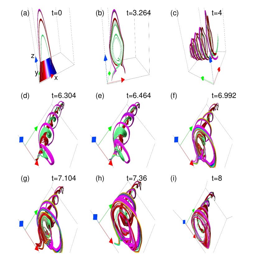
Figure 10: Panels (a) to (i) show the topology of MFLs in their evolution for $\delta_{i}/L=0.04$ under the Hall forcing. Important is the similarity of the dynamics leading to the formation of primary MFR which generates at a similar instant as the primary MFR in the absence of the Hall forcing. (A combined animation of Figure 9 and Figure 10 is available.)

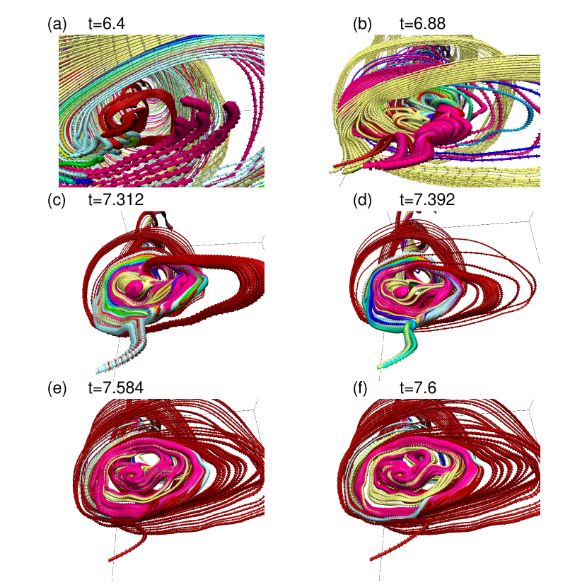
Figure 11: Sequence of MFL evolution under the Hall forcing ($\delta_{i}/L=0.04$ case), zoomed to reveal intricate magnetic topologies generated by the MRs. Formation of the “figure 8” kind magnetic structures (panels (a) to panel (f))—the magnetic islands—can be seen clearly. Importantly, such intricate topologies are absent in the MFR evolution without the Hall forcing. (An animation of the evolution from $t=7.312$ onwards is available.)

The MFL evolution for $\delta_{i}/L=0.04$ is exhibited in Figure 10. The selected value is on the order of the coronal value quoted in Introduction and optimizes the computation. The primary MFR develops at $t=4$, which is similar to the instant at which the primary MFR was generated for the $\delta_{i}/L=0$ case. The overall dynamics leading to the primary MFR also remains similar to the one without the Hall forcing. The similar dynamics and the near-simultaneity in the onset of the the primary MFR in both cases indicate the large scale dynamics, i.e., the dynamics before or away from MRs, to be insensitive to the particular Hall forcing. However, there are conspicuous differences between the MHD and HMHD realizations of the MFR morphology. In the HMHD case the primary MFR undergoes multiple internal MRs highlighted in Figure 11, leading to MFL morphologies which when projected favorably look like magnetic islands similar to those found in the sinusoidal simulation. A swirling motion is also observed; cf. panels (a) to (f) of Figure 11 (better visualized in the animation). Noteworthy, swirling motion during evolution of a prominence eruption has been observed (Pant et al., 2018).

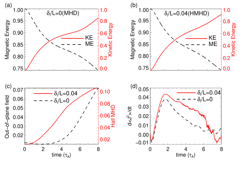
Figure 12: Panels (a) and (b) show the evolution of normalized (with the initial total energy) grid averaged magnetic energy (black dashed curve) and kinetic energy (red solid curve) for $\delta_{i}/L=0$ (MHD) and $\delta_{i}/L=0.04$ (HMHD) respectively. Panel (c) shows the evolution of grid averaged out-of-plane magnetic field for $\delta_{i}/L=0$ (MHD) with black dashed curve and $\delta_{i}/L=0.04$ (HMHD) with red solid curve respectively. Also in Panels (a) to (c), the scales for the solid and the dashed curves are spaced at right and left respectively. Panel (d) represents grid averaged rate of change of total current density for $\delta_{i}/L=0$ (black dashed curve) and $\delta_{i}/L=0.04$ (red solid curve) respectively. Important are the generation of the out-of-plane magnetic field along with small but abrupt changes in time derivative of the total volume current density in HMHD simulation.

To complete the analyses, we plot the overall evolution of magnetic and kinetic energies, amplitude of the out-of-plane field and the rate of change of the total volume current density in panels (c) and (d) of the Figure 12. The similarity of the energy curves in the presence and absence of the Hall forcing is a reminiscent of the fact that the Hall term does not affect the system energetics directly. Importantly, the out-of-plane magnetic field (approximated by the axial magnetic field $B_{y}$) is larger than that in the absence of the Hall forcing, in accordance with the expectation. Further, contrary to its smooth variation in the MHD case, the rate of change of total volume current density in HMHD goes through small but abrupt changes. Such abrupt changes may correspond to a greater degree of impulsiveness (Bhattacharjee, 2004).

To check the dependence of the above findings on the grid resolution, we have carried out auxiliary simulations with $32\times 32\times 64$ grid resolution, spanning the same physical domain with all the other parameters kept identical (not shown). The findings are similar to those at the higher resolution. In particular, they evince the nearly simultaneous formation of the primary MFR, with and without the Hall forcing, through the similar dynamical evolution. Also, breakage of the primary MFR through internal MRs is found in presence of Hall forcing whereas no such breakage is seen in the absence of the Hall forcing. The identical dynamics in two separate resolutions indicate the findings to be independent of the particular resolution used.

4 Summary

The Eulerian-Lagrangian model EULAG-MHD has been extended to the HMHD regime, by modifying the induction equation to include the Hall term. Subsequently, benchmarking is done with an initially sinusoidal magnetic field, symmetric in the $y$-direction of the employed Cartesian coordinate system. The choice of the field is based on its simplicity and non-force-free property to exert Lorentz force on the magnetofluid at $t=0$. Moreover, the selected field provides an opportunity to independently verify the physics of HMHD without repeating the more traditional computations related to the Harris equilibrium or the GEM challenge. Simulations are carried out in the absence and presence of the Hall term. In the absence of the Hall term the magnetic field maintains its symmetry as MRs generate magnetic flux tubes made by disjoint MFLs. With the Hall term, the evolution becomes asymmetric and 3D due to the development of magnetic field which is directed out of the reconnection plane. This is in concurrence with earlier simulations. Along with the flux tube, MRs also generate magnetic flux rope in the HMHD. When viewed along the $-y$ direction, the rope and the tube appear as magnetic islands. Further evolution, leads to breakage of the primary islands into secondary islands and later, their coalescence. The results, overall, agree with the existing scenarios of Hall-reconnection based on physical arguments and other recent simulations including those on the GEM challenge. An important finding is the formation of complex 3D magnetic structures which can not be apprehended from 2D models or calculations although their projections agree with the latter. Alongside, we have numerically explored the Whistler mode propagation vis-a-vis its analytical model and found the two to be matching reasonably well.

We have further carried out simulations where the EULAG-MHD is used to simulate the onset and dynamics of a MFR initiating from a sheared magnetic arcade. Such computations are relevant in understanding the solar eruptions. Simulations conducted with and without the Hall term are compared once more. Once again a reasonable maintenance of symmetry is observed in the standard MHD simulation, whereas a clear symmetry-breaking—leading to generation of 3D magnetic structures—appears to be a signature of the Hall effect. In HMHD the MFR evolves through a series of complex geometries while rotating along its axis. When viewed favorably, it appears to contain structures like the “figure 8”, which is the result of internal reconnection within MFR. Notably, the magnetic and kinetic energies, in the presence and absence of the Hall forcing, behave almost identically—consistent with the theoretical understanding that the Hall term does not directly change the magnetic energy. Moreover, we have performed and analyzed the simulations with half the resolution and found their results to be similar to the reference results. The same process of the primary MFR formation and its further breakage through multiple internal magnetic reconnections does confirm the independency of the results on the grid resolution.

Overall, the extended EULAG-MHD is giving results in accordance with the theoretical expectations and other contemporary simulations. The Hall simulation documenting activation of a magnetic flux rope from initial sheared arcade field lines is of particular importance and is a new entry to the ongoing research. It shows that Hall magnetohydrodynamics can account for a richer complexity during evolution of the rope by breaking any pre-existing 2D symmetry, thus opening another degree of freedom for the MFL evolution. The resulting local breakage of the rope is intriguing by itself and calls for further research.

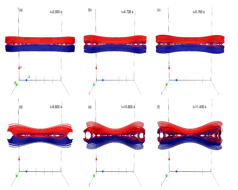
Figure 8: MFL evolution for $d_{0}=2$ (HMHD), projected on $y$ constant plane. Panel (a) depicts development of two primary magnetic islands. Panels (b) and (c) show their further breakage into secondary islands. Panels (d) to (f) show generation of an X type neutral point by subsequent merging of the two islands. (An animation of this figure is available.)

References

- Alfvén (1942) Alfvén, H. 1942, Nature, 150, 405
- Aschwanden (2005) Aschwanden, M. J. 2005, Physics of the Solar Corona. An Introduction with Problems and Solutions (2nd edition)
- Bhattacharjee (2004) Bhattacharjee, A. 2004, ARA&A, 42, 365
- Bhattacharyya et al. (2010) Bhattacharyya, R., Low, B. C., & Smolarkiewicz, P. K. 2010, Physics of Plasmas, 17, 112901
- Birn et al. (2001) Birn, J., et al. 2001, J. Geophys. Res., 106, 3715
- Charbonneau & Smolarkiewicz (2013) Charbonneau, P., & Smolarkiewicz, P. K. 2013, Science, 340, 42
- Chen (2011) Chen, P. F. 2011, Living Reviews in Solar Physics, 8, 1
- Choudhuri (1998) Choudhuri, A. R. 1998, The physics of fluids and plasmas : an introduction for astrophysicists
- Freidberg (1982) Freidberg, J. P. 1982, Reviews of Modern Physics, 54, 801
- Grinstein et al. (2007) Grinstein, F., Margolin, L., & Rider, W. 2007, Implicit Large Eddy Simulation: Computing Turbulent Fluid Dynamics, Cambridge University Press
- Huba (2003) Huba, J. D. 2003, Hall Magnetohydrodynamics - A Tutorial, ed. J. Büchner, M. Scholer, & C. T. Dum (Berlin, Heidelberg: Springer Berlin Heidelberg), 166
- Huba & Rudakov (2002) Huba, J. D., & Rudakov, L. I. 2002, Physics of Plasmas, 9, 4435
- Kumar & Bhattacharyya (2011) Kumar, D., & Bhattacharyya, R. 2011, Physics of Plasmas, 18, 084506
- Kumar et al. (2017) Kumar, S., Bhattacharyya, R., Dasgupta, B., & Janaki, M. S. 2017, Physics of Plasmas, 24, 082902
- Kumar et al. (2016) Kumar, S., Bhattacharyya, R., Joshi, B., & Smolarkiewicz, P. K. 2016, ApJ, 830, 80
- Kumar et al. (2015) Kumar, S., Bhattacharyya, R., & Smolarkiewicz, P. K. 2015, Physics of Plasmas, 22, 082903
- Ma & Bhattacharjee (2001) Ma, Z. W., & Bhattacharjee, A. 2001, J. Geophys. Res., 106, 3773
- Mozer et al. (2002) Mozer, F. S., Bale, S. D., & Phan, T. D. 2002, Phys. Rev. Lett., 89, 015002
- Nayak et al. (2019) Nayak, S. S., Bhattacharyya, R., Prasad, A., Hu, Q., Kumar, S., & Joshi, B. 2019, ApJ, 875, 10
- Nayak et al. (2020) Nayak, S. S., Bhattacharyya, R., Smolarkiewicz, P. K., Kumar, S., & Prasad, A. 2020, ApJ, 892, 44
- Pant et al. (2018) Pant, V., Datta, A., Banerjee, D., Chandrashekhar, K., & Ray, S. 2018, The Astrophysical Journal, 860, 80
- Parker (1994) Parker, E. N. 1994, Spontaneous current sheets in magnetic fields : with applications to stellar x-rays. International Series in Astronomy and Astrophysics, 1
- Prasad et al. (2018) Prasad, A., Bhattacharyya, R., Hu, Q., Kumar, S., & Nayak, S. S. 2018, ApJ, 860, 96
- Prasad et al. (2017) Prasad, A., Bhattacharyya, R., & Kumar, S. 2017, ApJ, 840, 37
- Priest (2014) Priest, E. 2014, Magnetohydrodynamics of the Sun
- Priest & Forbes (2000) Priest, E., & Forbes, T. 2000, Magnetic Reconnection
- Prusa et al. (2008) Prusa, J., Smolarkiewicz, P., & Wyszogrodzki, A. 2008, Computers & Fluids, 37, 1193
- Shi et al. (2019) Shi, C., Tenerani, A., Velli, M., & Lu, S. 2019, ApJ, 883, 172
- Shibata & Tanuma (2001) Shibata, K., & Tanuma, S. 2001, Earth, Planets, and Space, 53, 473
- Smolarkiewicz (2006) Smolarkiewicz, P. K. 2006, International Journal for Numerical Methods in Fluids, 50, 1123
- Smolarkiewicz & Charbonneau (2013) Smolarkiewicz, P. K., & Charbonneau, P. 2013, Journal of Computational Physics, 236, 608
- Sonnerup (1979) Sonnerup, B. U. Ö. 1979, Magnetic field reconnection, Vol. 3 45
- Westerberg & Åkerstedt (2007) Westerberg, L. G., & Åkerstedt, H. O. 2007, Physics of Plasmas, 14, 102905