Contextuality based quantum conferencing

Abstract

Nonlocality inequalities for multi-party systems act as contextuality inequalities for single qudit systems of suitable dimensions [Heywood and Redhead, Found. Phys., 13(5), 481–499, 1983; Abramsky and Brandenburger, New J. Phys., 13(11), 113036, 2011]. In this paper, we propose the procedure for adaptation of nonlocality-based quantum conferencing protocols (NQCPs) to contextuality-based QCPs (CQCPs). Unlike the NQCPs, the CQCPs do not involve nonlocal states. As an illustration of the procedure, we present a QCP based on Mermin’s contextuality inequality. As a significant improvement, we propose a QCP based on CHSH contextuality inequality involving only four-dimensional states irrespective of the number of parties sharing the key. The key generation rate of the latter is twice that of the former. Although CQCPs allow for an eavesdropping attack which has no analog in NQCPs, a way out of this attack is demonstrated. Finally, we examine the feasibility of experimental implementation of these protocols with orbital angular momentum (OAM) states.

1 Introduction

The surge of interest in nonclassical aspects of quantum mechanics owes largely to the applications that they offer. Examples include search algorithms and quantum computing algorithms Grover ; deutschjozsa which provide computational speedups as compared to their classical counterparts. There also exist altogether novel applications such as quantum teleportation, superdense coding Bennett92a ; Bennett93 , and quantum key distribution protocols. In particular, fundamental features of quantum mechanics were first applied in quantum key distribution (QKD) Bennett84 ; Ekert91 ; namkung2020generalized . Thanks to the no-cloning theorem Wootters82 and the existence of non-orthogonal bases, QKD protocols are unconditionally secure. In the celebrated Ekert protocol Ekert91 , nonlocal states are employed for key distribution. Though these states are not essential in the generation and certification of the key, they play a crucial role in device-independent QKD protocols Vazirani14 . Since nonlocality is a costly resource, other QKD protocols have been proposed whose security analyses are based on monogamy relations of other quantum features, e.g., quantum discord su2014Guassiandiscord ; pirandola2014quantum and contextuality Troupe15 ; Singh17 . Additionally, the Kochen-Specker theorem has been identified as a condition for secure QKD in Nagata05 . The contextuality-based QKD protocols proposed in Troupe15 ; Singh17 can be employed to generate a secure key between two parties.

It has been noticed Heywood83 ; Mermin90a ; Guhne10 that the CHSH nonlocality inequality for a bipartite system detects contextuality in a single system. The interrelation between nonlocality and contextuality has been further placed on a firm ground using the sheaf-theoretic framework Abramsky11 . In short, nonlocality inequalities can be adapted to detect contextuality in a single system of suitable dimensions. The reason underlying this adaption is the isomorphism of Hilbert spaces of identical dimensions.

In this paper, we exploit the formal equivalence between nonlocality and contextuality to propose QCPs based entirely on contextuality, corresponding to any NQCP. However, our protocols are significantly different from the NQCPs. The isomorphism between the Hilbert spaces extends only upto the states and the algebra of the observables. The implementation of the QCPs and security against eavesdropping are completely different. In short, the CQCPs are not just mathematical analogs of NQCPs. So, the similarity and contrast of the two QCPs are schematically shown in figures (1) and (2) respectively. Particular attention may be paid to “masking transformations” $\mathbb{U}$, which are employed for security, in figure (2). It is discussed in detail in section (5).

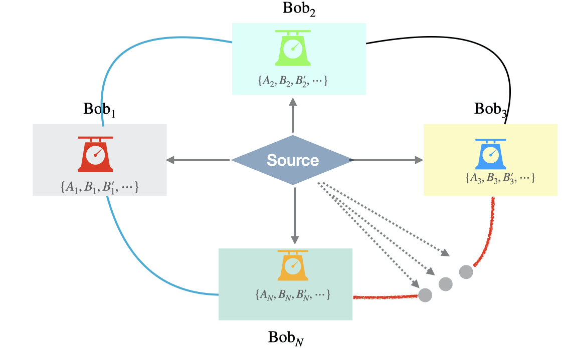
Figure 1: Pictorial representation of QCP based on nonlocality inequality: an $N$-party nonlocal state is shared among $N$ parties, viz., ${\rm Bob}_{1},\cdots,{\rm Bob}_{N}$ who perform random measurements of $A_{k},B_{k},B_{k}^{\prime}\cdots;1\leq k\leq N$. The outcomes of $B_{k},B_{k}^{\prime}\cdots$ are revealed on a classical channel to check for violation of nonlocality inequality and those of $A_{k}$ are used to generate the key.

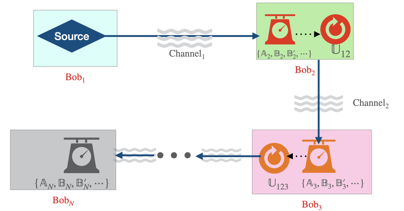
Figure 2: Pictorial representation of QCP based on contextuality: ${\rm Bob}_{1}$ has a source to produce a $d^{N}$– dimensional state. Bob_k performs random measurement of one of the observables from the set $\{\mathbb{A}_{k},\mathbb{B}_{k},\mathbb{B}_{k}^{\prime},\cdots\}$ and thereafter, performs an arbitrary unitary transformation $\mathbb{U}_{1\cdots k}$ to make the protocol resilient against such attacks in which Eve’s observables commute with those of subsequent Bobs. The transformed state is then sent to Bob_k+1. The wavy lines in the figure represent possible noise in the channel.

We propose two classes of CQCPs. In the first class, a higher dimensional state is sent from the first party to the last party sequentially. In the second class, the parties are divided into partially overlapping groups and a relatively lower dimensional state is used for sharing the key among different groups. To illustrate these two classes, we have explicitly described QCPs based on Mermin’s contextuality inequality and CHSH contextuality inequality respectively.

Since all these protocols involve higher dimensional states, orbital angular momentum (OAM) states of light seem to be natural candidates for their implementation. There have been numerous recent advances in the generation beijersbergen94 ; Heckenberg92 and manipulation of higher dimensional OAM states of light, which provide an edge to quantum information processing with higher dimensional states Mair01 ; leach2002measuring ; berkhout2010efficient ; Dada11 ; Fickler12 ; malik2014direct ; zhou2016orbital ; yin2017 ; erhard18 . Noting this, we briefly outline how CQCPs may possibly be realised experimentally using OAM states.

The paper is organised as follows: in section (2), we set up the notation to be used in the paper, for an uncluttered discussion. In section (3), to make the discussion easier, the properties probed by CHSH contextuality inequality in a single system have been discussed. Section (4) develops the procedure, which is central to the paper, for obtaining CQCP from any NQCP. Section (5) discusses eavesdropping strategies and possible ways out. In section (6), we apply the procedure to propose the QCP based on Mermin’s contextuality inequality and discuss its key generation rate. Section (7) discusses how one can pinpoint the location of Eve. In section (8), the QCP based on CHSH contextuality inequality and its key generation rate have been discussed. Section (9) presents a possibility of how the protocols may be implemented using orbital angular momentum (OAM) states of light. In section (10), effects of imperfect preparation of the states and noisy measurements on the QCP based on Mermin’s and CHSH contextuality inequality are studied. Section (11) summarises the paper with concluding remarks.

2 Notation

In this section, we set up the notation to be used henceforth in the paper:

1. 1. Observables acting on a multi-party system will be represented by $A_{k},A^{\prime}_{k},\cdots$. The party which measures these observables is represented in the subscript.

   2. The corresponding observables acting on a single qudit system will be represented by $\mathbb{A}_{k},\mathbb{A}_{k}^{\prime},\cdots$.

2. Mapping between bases:
   Let

   $$\mathfrak{B}_{1} \equiv\{|j_{1}j_{2}\cdots j_{N}\rangle;j_{k}\in\{0,1,\cdots,d-1\},1\leq k\leq N\};$$ (1)

   $$\mathfrak{B}_{2} \equiv\{|0\rangle,|1\rangle,\cdots,|D-1\rangle\},$$

   where $\mathfrak{B}_{1}$ is a basis for the tensor product space of $N$ $d$-dimensional Hilbert spaces $({\cal H}^{d})^{\otimes N}$. Simialarly, $\mathfrak{B}_{2}$ is a basis for a Hilbert space, ${\cal H}^{D}$, of dimension $D\equiv d^{N}$. Since $({\cal H}^{d})^{\otimes N}$ and ${\cal H}^{D}$ are isomorphic to each other, we set up the following bijective mapping between the bases $\mathfrak{B}_{1}$ and $\mathfrak{B}_{2}$:

   $$|j_{1}\cdots j_{N}\rangle\leftrightarrow\Big{|}\sum_{k=1}^{N}d^{N-k}j_{k}\Big{\rangle}=\ket{j}.$$ (2)

3. Mapping of observables:
   The symbol $\mathbb{M}_{k}$ represents the observable having the same matrix representation in the basis $\mathfrak{B}_{2}$, as the observable $\mathbb{1}^{\otimes k-1}\otimes M_{k}\otimes\mathbb{1}^{\otimes N-k}$ has in the basis $\mathfrak{B}_{1}$. That is,

   $$\langle j|\mathbb{M}_{k}|l\rangle =\big{\langle}j_{1}\cdots j_{N}\big{|}\mathbb{1}^{\otimes k-1}\otimes M_{k}\otimes\mathbb{1}^{\otimes N-k}\big{|}l_{1}\cdots l_{N}\big{\rangle}.$$ (3)

   In particular, the projection operator corresponding to an eigenvalue $m$ of an operator $\mathbb{M}$ will be represented by ${\mathbb{\Pi}}_{\mathbb{M}}^{m}$.

4. We denote the states of multi-party systems by lowercase Greek letters $|\psi\rangle,|\xi\rangle,\cdots$ and the states of a single qudit by uppercase Greek letters $|\Psi\rangle,|\Xi\rangle,\cdots$.

5. Mapping of unitary transformations:
   

   1. Employing the mapping defined in equation (2), the unitary transformations performed by the $k^{th}$ party in a multi-party system, represented by $U_{k}$, are mapped to $\mathbb{U}_{k}$ in a single qudit, i.e.,

      $$\mathbb{1}^{\otimes k-1}\otimes U_{k}\otimes\mathbb{1}^{\otimes N-k}\leftrightarrow\mathbb{U}_{k}.$$ (4)

   2. Similarly, the unitary transformations performed on the combined space of $j^{th}$ and $k^{th}$ party, represented by $U_{jk}$, are mapped to $\mathbb{U}_{jk}$ in a single qudit system, i.e.,

      $$\mathbb{1}^{\otimes j-1}\otimes U_{jk}\otimes\mathbb{1}^{N-k}\leftrightarrow\mathbb{U}_{jk}.$$ (5)

      Similarly, the transformation acting on the combined space of first $k$ parties of a multiparty system, $U_{1\cdots k}$, is mapped to $\mathbb{U}_{1\cdots k}$ in a single qudit system straightforwardly, i.e.,

      $$U_{1\cdots k}\otimes{\mathbb{1}}^{N-k}\leftrightarrow\mathbb{U}_{1\cdots k}.$$ (6)

6. The symbols $X_{k},Y_{k},Z_{k}$ shall be reserved for the Pauli matrices acting over the space of the $k^{\rm th}$ qubit and their counterparts for a single qudit will be represented by $\mathbb{X}_{k},\mathbb{Y}_{k},\mathbb{Z}_{k}$.

7. Finally, we represent the sequential measurements of observables $A_{1},\cdots,A_{N}$, such that $A_{1}$ is measured first and $A_{N}$ is measured last, by the symbol $(A_{1}\cdots A_{N})$.

3 Relation between multi-party nonlocality and contextuality in a single qudit

Multi-party states that violate nonlocality inequalities also exhibit contextual behaviour, i.e., nonlocality and contextuality coexist in the multi-party states Guhne10 . However, multi-party nonlocality inequalities, with the mapping given in equation (2), can be adapted to detect contextuality in a single qudit system of suitable dimensions. In this section, for the purpose of pedagogy, we illustrate this with the example of CHSH inequality.

3.1 CHSH inequality as a contextuality inequality

CHSH inequality detects nonlocality in a bipartite system of arbitrary dimension Clauser69 . We show that the same inequality also detects contextuality. Consider a simple example of two-qubit systems. Let $\ket{\psi}$ be the singlet state of two-qubits, i.e., $|\psi\rangle=\frac{1}{\sqrt{2}}(|01\rangle-|10\rangle)$. Consider a set of three observables $\{X_{1},X_{2},Z_{2}\}$. Evidently, $[X_{1},X_{2}]=[X_{1},Z_{2}]=0$ but $[X_{2},Z_{2}]\neq 0$. We are interested in the following two contexts:
Context 1: $(X_{2}X_{1})$, i.e., $X_{2}$ is measured first followed by $X_{1}$. If the outcome of $X_{2}$ is $+1(-1)$, the outcome of $X_{1}$ is guaranteed to be $-1(+1)$.
Context 2: $(Z_{2}X_{1})$. Irrespective of the outcome of $Z_{2}$, which is $\pm 1$, the outcome of $X_{1}$ can be $+1$ or $-1$ with equal probability.
Thus, the outcome of $X_{1}$ depends on the observable with which it is measured, i.e., it depends on the context. Thus, CHSH nonlocality inequality also detects contextuality in a two-qubit system.

Of course, a single qudit cannot exhibit nonlocal behaviour. In what follows, we show how a similar contextual behaviour gets manifested in a single four-level system. Employing the following mapping between the bases of a two-qubit system and a single four level system,

$$|00\rangle\equiv|0\rangle;~{}|01\rangle\equiv|1\rangle;~{}|10\rangle\equiv|2\rangle;~{}|11\rangle\equiv|3\rangle,$$ (7)

the singlet state $|\psi\rangle$ gets mapped to $|\Psi\rangle$,

$$|\Psi\rangle=\frac{1}{\sqrt{2}}(|1\rangle-|2\rangle),$$ (8)

and the observables $X_{1},X_{2},Z_{2}$ map to the following observables:

$$X_{1}\mapsto \mathbb{X}_{1}=|0\rangle\langle 2|+|2\rangle\langle 0|+|1\rangle\langle 3|+|3\rangle\langle 1|$$

$$X_{2}\mapsto \mathbb{X}_{2}=|0\rangle\langle 1|+|1\rangle\langle 0|+|2\rangle\langle 3|+|3\rangle\langle 2|$$

$$Z_{2}\mapsto \mathbb{Z}_{2}=|0\rangle\langle 0|-|1\rangle\langle 1|+|2\rangle\langle 2|-|3\rangle\langle 3|.$$ (9)

Naturally, the isomorphism of Hilbert spaces extends to the algebra of operators.

We may consider the same contexts for $\mathbb{X}_{1},\mathbb{X}_{2},\mathbb{Z}_{2}$ with the state $|\Psi\rangle$ as considered for $X_{1},X_{2},Z_{2}$ with the singlet state $|\psi\rangle$.
Context 1 ($\mathbb{X}_{2}\mathbb{X}_{1}$): i.e., $\mathbb{X}_{2}$ is measured first followed by measurement of $\mathbb{X}_{1}$. If the outcome of $\mathbb{X}_{2}$ is $+1(-1)$, the outcome of $\mathbb{X}_{1}$ is guaranteed to be $-1(+1)$.
Context 2 ($\mathbb{Z}_{2}\mathbb{X}_{1}$): Irrespective of the outcome of $\mathbb{Z}_{2}$, the outcome of $\mathbb{X}_{1}$ will be $+1$ or $-1$ with equal probability.
The outcome of $\mathbb{X}_{1}$ depends on which observable has been measured before it, i.e., it depends on the context. So, the isomorphism extends to the contexts as well. Thus, CHSH inequality can be adapted to detect sequential contextuality in a single four-level system for which it can be referred to as CHSH contextuality inequality. Similarly, $N$–party Mermin’s nonlocality inequality can be referred to as Mermin’s contextuality inequality in a single qudit system of appropriate dimension Abramsky11 , as illustrated in appendix (A).

4 The procedure for obtaining contextuality-based QCP from any nonlocality-based QCP

In this section, we employ the formal equivalence between contextuality and nonlocality to develop the procedure to obtain a CQCP from a NQCP.

Let $\{A_{k},B_{k},B^{\prime}_{k},B^{\prime\prime}_{k},\cdots\}$ be a set of observables, acting over the $k^{\rm th}$ qudit of an $N$-qudit system. Any nonlocality inequality can be cast into the form Brunner14 ,

$$\centering\langle O\rangle\leq c,\@add@centering$$ (10)

where $O$ consists of sums of multilinears in the observables $B_{k},B^{\prime}_{k},B^{\prime\prime}_{k}$ and $c$ is a non-negative number. Consider a NQCP in which the violation of the inequality (10) acts as a security check and the outcomes of the observables $\{A_{1},\cdots,A_{N}\}$ are used to generate the shared secret key. The sets $\{A_{1},\cdots,A_{N}\}$ and $\{B_{1},B^{\prime}_{1},\cdots,B_{N},B^{\prime}_{N}\}$ may be partially overlapping or completely disjoint, examples being Ekert protocol Ekert91 and Mermin inequality based QKD protocol MABK respectively.

S. No.	NQCP	CQCP
1	All the observables are	All the observables are
	publicly announced.	publicly announced.
2	$|\psi\rangle:$ $N$–qudit nonlocal state	$|\Psi\rangle:$ a single $d^{N}$-dimensional
	simultaneously shared among $N$	reference state.
	parties viz., Bob${}_{1},\cdots,\rm{Bob}_{N}$.
3	Bobk randomly measures one of the observables from the set $\{A_{k},B_{k},B^{\prime}_{k},\cdots\}$.	a) Bob1 randomly prepares a state
		$|\Psi^{\prime}\rangle=\mathbb{U}_{1}{\mathbb{\Pi}}_{\mathbb{M}}^{{m}}|\Psi\rangle$, with a probability $\frac{1}{t}\langle\Psi|{\mathbb{\Pi}}_{\mathbb{M}}^{m}|\Psi\rangle$,
		where $\mathbb{M}$ is one of the observables from the set,
		$\{\mathbb{A}_{1},\mathbb{B}_{1},\mathbb{B}^{\prime}_{1},\cdots\}$, whose cardinality is $t$. The
		symbol $\mathbb{U}_{1}=e^{i(\alpha_{1}\mathbb{A}_{1}+\beta_{1}\mathbb{B}_{1}+\cdots)}$ represents an
		arbitrary unitary transformation, which commutes
		with observables of subsequent Bobs.
		b)   The state $|\Psi^{\prime}\rangle$ is sent to
		Bob2 who randomly measures one
		of the observables $\{\mathbb{A}_{2},\mathbb{B}_{2},\mathbb{B}^{\prime}_{2},\cdots\}$.
		c)   He performs an arbitrary transformation
		$\mathbb{U}_{12}$ (which commutes with the observables
		of subsequent Bobs) on the post-measurement
		state and sends the transformed state to Bob3.
		d) This process continues until BobN
		randomly measures one of the
		observables $\{\mathbb{A}_{N},\mathbb{B}_{N},\mathbb{B}^{\prime}_{N},\cdots\}$.
4	This process is repeated	This process is repeated
	for many rounds.	for many rounds.
5	The violation of nonlocality	The violation of contextuality
	inequality $\langle{O}\rangle\leq c\implies$	inequality $\langle\mathbb{O}\rangle\leq c\implies$
	No eavesdropping (and vice versa).	No eavesdropping (and vice versa).
6	If the inequality is violated,	If the inequality is violated,
	the outcomes of $A_{1},\cdots,A_{N}$	the outcomes of $\mathbb{A}_{1},\cdots,\mathbb{A}_{N}$
	act as a shared key.	act as a shared key.

Table 1: Procedure for obtaining a CQCP from NQCP.

Let the corresponding contextuality inequality and the sets of observables be,

$$\langle\mathbb{O}\rangle\leq c,$$ (11)

and $\{\mathbb{A}_{1},\cdots,\mathbb{A}_{N}\}$, $\{\mathbb{B}_{k},\mathbb{B}_{k}^{\prime},\mathbb{B}_{k}^{{}^{\prime\prime}},\cdots\}$ respectively for a single qudit system of dimension $d^{N}$. That is to say, the observables $\mathbb{A}_{k},\mathbb{B}_{k}$ and $A_{k},B_{k}$ have the same representations in the bases $\{|0\rangle,\cdots,|d^{N}-1\rangle\}$ and $\{|j_{1}\cdots j_{N}\rangle;j_{k}\in\{0,1,\cdots,d-1\},1\leq k\leq N\}$ respectively.

The steps to obtain the corresponding CQCP are neatly summarised in table (1), and are further employed to propose the QCP based on Mermin’s contextuality inequality in the section (6).

In the step 3(a) of table (1), we have incorporated multiple operations into a single step. It is possible because a state is to be sent from Bob₁ to Bob₂ after measurement and necessary transformation. Bob₁ has no need to prepare a state $\ket{\Psi}$ first and then perform measurement and transformation over it. Instead, he can directly prepare a state $\ket{\Psi^{\prime}}$ to be sent to Bob₂ which saves a lot of cost.

5 Security Analysis

As we have seen in table (1), some additional steps are performed in CQCPs. These steps are needed to make the CQCPs resilient against eavesdropping. As the physical systems employed are completely different, the isomorphism between the two Hilbert spaces (viz., ${\cal H}^{d^{\otimes N}}{\rm and}~{}{\cal H}^{d^{N}}$) does not extend to eavesdropping strategies, and, hence, not to the security analyses. In this section, we discuss the security analyses of CQCPs for measurement-resend attacks by an eavesdropper.

Evidently, in the CQCPs, the measurement operators of all Bobs are mutually commuting. So, if Eve is present, say, between $k^{\rm th}$ and $(k+1)^{\rm th}$ Bob, her measurement operators may either commute or non-commute with those of the subsequent Bobs. In the latter case, any tampering by Eve gets reflected in the non-violation of contextuality inequality by the maximal amount. The former case, however, eludes a violation of contextuality inequality and Eve’s tampering goes undetected. This case is unique to our protocols and merits a careful study in order to make our protocols robust against eavesdropping.

Assume that Eve measures observables from the set $\{\mathbb{A}_{\alpha},\mathbb{B}_{\alpha},\mathbb{B}^{\prime}_{\alpha},\cdots;1\leq\alpha\leq k\}$, which naturally commute with those of $(k+1)^{\rm th}$ to $N^{\rm th}$ Bob. Measurements of these observables by Eve do not affect the outcomes of the observables of subsequent Bobs. Thus, there is no effect of these measurements on the violation of contextuality inequality. In this manner, Eve obtains full information about the key by choosing appropriate observables and still goes undetected. This point is further made more explicit with an example in appendix (B). To obstruct Eve from obtaining any information, we propose a way out as explained in the following subsection.

5.1 The wayout: masking transformations

In order to make our protocol resilient against this attack, the following strategy may be adopted. After making a measurement on the state, each Bob performs a random unitary transformation with the sole condition that it commutes with the observables of subsequent Bobs. That is to say, Bob₁ prepares a state and performs a random unitary transformation $\mathbb{U}_{1}$ generated by the observables accessed by him. Then, Bob₂ makes his measurement and performs a random unitary transformation $\mathbb{U}_{12}$, generated by the observables accessed by both him and his predecessor. This chain is continued with every Bob but the last one. Thus, Bob_k makes his measurement and performs a unitary transformation $\mathbb{U}_{1\cdots k}$ generated by the observables accessed by him and all his predecessors. These random unitary transformations are termed as masking transformations as they mask the information about the outcomes of the observables of the preceding Bobs. Thus, Eve would be none the wiser about the key.

We now make the procedure explicit for the protocol presented in table (1). Bob₁, after preparing the state, say, $\ket{\Psi_{1}}={\mathbb{\Pi}}_{\mathbb{A}_{1}}^{a_{1}}\ket{\Psi}$, performs a masking transformation,

$$\mathbb{U}_{1}=\exp{[{i(\beta_{1}\mathbb{B}_{1}+\beta^{\prime}_{1}\mathbb{B}^{\prime}_{1}+\cdots)}]};~{}\beta_{1},\beta_{1}^{\prime}\in\mathbb{R}.$$ (12)

The transformed state, $\ket{\Psi^{\prime}}=\mathbb{U}_{1}|\Psi_{1}\rangle$, is transmitted to Bob₂. Now, even if Eve intercepts the state on its way from Bob₁ to Bob₂ and performs a measurement of the observable $\mathbb{A}_{1}$, she does not gain information about the key. This is because the transformation $\mathbb{U}_{1}$ has changed the information about the outcome of observable $\mathbb{A}_{1}$, and thus, masks the information about the measurement of Bob₁. This feature holds at all the steps because each Bob (excluding the last one) performs a random unitary transformation. This justifies the nomenclature masking for these transformations.

Masking transformations, together with the violation of contextuality inequality, assure the security of the protocol against such attacks.

5.2 Invariance of context under masking transformations

In what follows, we provide an explicit proof that masking transformations do not change the context and hence correlations in the outcomes of observables are intact. This is made possible by the fact that masking transformations performed by Bob_k commute with the observables of subsequent Bobs (i.e., Bob${}_{k+1},\cdots,$ Bob${}_{N})$ as guaranteed by the definition of $\mathbb{U}_{1}$ in equation (12) (which commutes with observables of Bob${}_{2},\cdots,$ Bob_N). An explicit proof follows.
Proof: The proof consists of three parts. In the first part, we show that the expectation values of observables of subsequent Bobs remain invariant after the masking transformation. In the second part, we show that the eigenstates of the observables of the subsequent Bobs lie within the same eigenspace even after the masking transformation. In the last part, we show that correlations among different observables remain invariant.

(i) Invariance of expectation value of observables : Let $\ket{\Phi_{k}}$ be the post–measurement state of Bob_k which changes to $\ket{\Psi_{k}}$ after a masking transformation $\mathbb{U}_{1\cdots k}$ has been performed by Bob_k, i.e.,

$$|\Psi_{k}\rangle=\mathbb{U}_{1\cdots k}|\Phi_{k}\rangle.$$ (13)

Note that, by definition, the masking transformation $\mathbb{U}_{1\cdots k}$ commutes with the observables of the subsequent Bobs, i.e., (Bob${}_{k+1},\cdots,$ Bob_N). As per the protocol, Bob_k+1 will perform a measurement of one of the observables from the set $\{\mathbb{A}_{k+1},\mathbb{B}_{k+1},\mathbb{B}^{\prime}_{k+1},\cdots\}$. We explicitly consider the observable $\mathbb{B}_{k+1}$ for which,

$$\langle\Psi_{k}|\mathbb{B}_{k+1}|\Psi_{k}\rangle=\langle\Phi_{k}|\mathbb{U}^{\dagger}_{1\cdots k}\mathbb{B}_{k+1}\mathbb{U}_{1\cdots k}|\Phi_{k}\rangle=\langle\Phi_{k}|\mathbb{B}_{k+1}|\Phi_{k}\rangle.$$ (14)

Since the choice of $\mathbb{B}_{k+1}$ is arbitrary, this holds true for any observable of subsequent Bobs, including projection operators. Hence, all the probabilities and expectation values of the subsequent Bobs remain invariant under this transformation.

(ii) Invariance of outcomes of observables of subsequent Bobs: In the protocol presented in the section (4), a key is generated when all the $N-$ Bobs perform measurements of their respective observables from the set $\{\mathbb{A}_{1},\mathbb{A}_{2},\cdots,\mathbb{A}_{k},\mathbb{A}_{k+1},\cdots,\mathbb{A}_{N}\}$. Given that, the post-measurement states of Bob_k are eigenstates of the observables of the subset $\{\mathbb{A}_{k+1},\cdots,\mathbb{A}_{N}\}$. We show that the states after the masking transformations continue to be the eigenstates of these observables with the same eigenvalues.

Suppose that the post-measurement state $|\Phi_{k}\rangle$ of Bob_k is an eigenstate of $\mathbb{A}_{k+1}$ with eigenvalue $a_{k+1}$. Let $\ket{\Psi_{k}}$ be the state obtained after performing the masking transformation $\mathbb{U}_{1\cdots k}$ on $\ket{\Phi_{k}}$. We show that the state $|\Psi_{k}\rangle$ is also an eigenstate of $\mathbb{A}_{k+1}$ with the same eigenvalue $a_{k+1}$ as follows:

$$\mathbb{A}_{k+1}|\Psi_{k}\rangle=\mathbb{A}_{k+1}\mathbb{U}_{1\cdots k}|\Phi_{k}\rangle=\mathbb{U}_{1\cdots k}\mathbb{A}_{k+1}|\Phi_{k}\rangle=a_{k+1}\mathbb{U}_{1\cdots k}|\Phi_{k}\rangle=a_{k+1}|\Psi_{k}\rangle.$$

The above equation holds due to the commutativity of $\mathbb{U}_{1\cdots k}$ with the observables of subsequent Bobs. This clearly shows that if a state $\ket{\Phi_{k}}$ is an eigenstate of observable, so is the state $\ket{\Psi_{k}}$, which proves the assertion. Since the choice of the observable $\mathbb{A}_{k+1}$ is arbitrary, it implies that this result holds for any observable.

(iii) Invariance of correlations: We prove this by demonstrating the invariance of correlation among three Bobs. It admits a straightforward generalization to $N-$ Bobs. Suppose that Bob₁ measures $\mathbb{\Pi}_{\mathbb{B}_{1}}^{b_{1}}$ on the state $\ket{\Psi}$, followed by a masking transformation $\mathbb{U}_{1}$ (generated by the observables accessible to Bob₁). Thereafter, Bob₂ measures $\mathbb{\Pi}_{\mathbb{B}_{2}}^{b_{2}}$, followed by a masking transformation $\mathbb{U}_{12}$ (generated by the observables of Bob₁ and Bob₂). Finally, Bob₃ measures $\mathbb{\Pi}_{\mathbb{B}_{3}}^{b_{3}}$, followed by a masking transformation $\mathbb{U}_{123}$. The state, after this process, is given by,

$$\mathbb{U}_{123}{\mathbb{\Pi}}_{\mathbb{B}_{3}}^{b_{3}}\mathbb{U}_{12}{\mathbb{\Pi}}_{\mathbb{B}_{2}}^{b_{2}}\mathbb{U}_{1}{\mathbb{\Pi}}_{\mathbb{B}_{1}}^{b_{1}}|\Psi\rangle.$$ (15)

The correlation in the three outcomes is given by,

$$\langle\Psi|\mathbb{\Pi}_{\mathbb{B}_{1}}^{b_{1}}\mathbb{U}^{\dagger}_{1}\mathbb{\Pi}_{\mathbb{B}_{2}}^{b_{2}}\mathbb{U}^{\dagger}_{12}\mathbb{\Pi}_{\mathbb{B}_{3}}^{b_{3}}\mathbb{U}_{123}^{\dagger}\mathbb{U}_{123}{\mathbb{\Pi}}_{\mathbb{B}_{3}}^{b_{3}}\mathbb{U}_{12}{\mathbb{\Pi}}_{\mathbb{B}_{2}}^{b_{2}}\mathbb{U}_{1}{\mathbb{\Pi}}_{\mathbb{B}_{1}}^{b_{1}}|\Psi\rangle=\langle\Psi|\mathbb{\Pi}_{\mathbb{B}_{1}}^{b_{1}}\mathbb{\Pi}_{\mathbb{B}_{2}}^{b_{2}}\mathbb{\Pi}_{\mathbb{B}_{3}}^{b_{3}}|\Psi\rangle.$$ (16)

The above equation follows because of the commutativity among observables of different Bobs (in this case $\mathbb{B}_{1},\mathbb{B}_{2},\mathbb{B}_{3}$) and that of the masking transformations with those of subsequent Bobs, i.e., $[\mathbb{U}_{1},\mathbb{\Pi}_{\mathbb{B}_{j}}^{b_{j}}]=0,~{}j=2,3$; $[\mathbb{U}_{12},\mathbb{\Pi}_{\mathbb{B}_{3}}^{b_{3}}]=0$ and, $[\mathbb{B}_{i},\mathbb{B}_{j}]=0,~{}i,j=1,2,3$. Thus, correlations remain intact after the application of a masking transformation.

The three results together show that masking transformations do not change the context. Thus, there is no effect of masking transformations either on correlations in a key or on the violation of contextuality inequality.

6 QCP based on Mermin’s contextuality inequality

As the first illustration of the procedure mentioned in table (1), we explicitly lay down the QCP based on Mermin’s contextuality inequality Abramsky11 for distributing a key among $N$ parties, viz., Bob${}_{1},\cdots,$ $\rm{Bob}_{N}$. Each Bob can choose an observable from a set of three dichotomic observables, i.e., Bob_k can choose from the set,

$${\cal S}_{k}\equiv\{\mathbb{X}_{k},\mathbb{Y}_{k},\mathbb{Z}_{k}\},~{}1\leq k\leq N.$$ (17)

Given these observables, Mermin’s contextuality inequality takes the form,

$$\mathbb{M}_{N} =\frac{1}{2i}\Bigg{|}\bigg{\langle}\prod_{k=1}^{N}(\mathbb{X}_{k}+i\mathbb{Y}_{k})-\prod_{k=1}^{N}(\mathbb{X}_{k}-i\mathbb{Y}_{k})\bigg{\rangle}\Bigg{|}\leq c$$

$$c =2^{N/2},\quad N={\rm even},$$ (18)

$$=2^{\frac{N-1}{2}},\quad N={\rm odd}.$$

Now, we are set to establish the protocol as per the procedure laid down in the preceding section:

1. All the observables are publicly announced.

2. Let $|\Psi_{M}\rangle=\frac{1}{\sqrt{2}}(|0\rangle+i|2^{N}-1\rangle)$ be the reference state. Bob₁ randomly prepares a state $|\Psi^{\prime}_{M}\rangle$, obtained by a random measurement of one of the observables $\mathbb{O}$ from the set ${\cal S}_{1}$ on $|\Psi_{M}\rangle$ with an equal probability, followed by a masking transformation $\mathbb{U}_{1}$. That is, $|\Psi^{\prime}_{M}\rangle=\mathbb{U}_{1}\mathbb{\Pi}_{\mathbb{O}}^{o}|\Psi_{M}\rangle$, $\mathbb{O}\in{\cal S}_{1}$. Then, he sends the state $|\Psi^{\prime}_{M}\rangle$ to Bob₂.

3. Bob₂ randomly measures any one of the observables from the set ${\cal S}_{2}$ and performs a masking transformation $\mathbb{U}_{12}$ (which can be generated using the set of observables of first two Bobs) on the post-measurement state. Thereafter, he sends the transformed state to Bob₃.

4. This process will continue till Bob_N performs his measurement. This concludes the first round.

5. This procedure is repeated for many rounds.

6. After many such rounds are completed, the choices of observables are revealed for each round.

7. The outcomes of such rounds, in which all the $N$-Bobs choose their respective observables from the set $\{\mathbb{Z}_{1},\mathbb{Z}_{2},\cdots,\mathbb{Z}_{N}\}$, are not revealed.

8. The outcomes of rounds, in which all the $N$-Bobs choose their respective observable from the set $\{(\mathbb{X}_{1},\mathbb{Y}_{1}),\cdots,(\mathbb{X}_{N},\mathbb{Y}_{N})\}$, are revealed. This data is used to check violation of Mermin’s contextuality inequality given by (6).

9. The outcomes of other rounds are discarded.

10. If inequality (6) is violated, it implies the absence of eavesdropping and the sets of outcomes of $\mathbb{Z}_{k}$ work as a shared secure key.

11. If inequality (6) is not violated, the presence of eavesdropping is indicated.

A pictorial representation of procedure outlined is shown in figure (3).

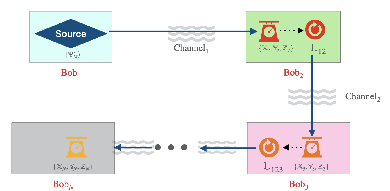
Figure 3: Schematic representation of Mermin’s CQCP.

6.1 Key generation rate

The key consists of outcomes of only those rounds in which all the $N$-Bobs choose their respective observables from the set $\{\mathbb{Z}_{1},\mathbb{Z}_{2},\cdots,\mathbb{Z}_{N}\}$. Since Bob_k randomly chooses one of the observables from the set $\{\mathbb{X}_{k},\mathbb{Y}_{k},\mathbb{Z}_{k}\}$, the probability for the event which generates the key is $\dfrac{1}{3^{N}}$. The Shannon information for the above protocol is 1 bit. So, the average key generation rate is $\dfrac{1}{3^{N}}$ bit. We stress that if one takes into account only the sifted data as is usually done, the key generation rate is 1 bit.

7 Can the location of Eve be pinpointed?

Violation of Mermin’s contextuality inequality by all the $N$-Bobs assures the secrecy of the shared key, contingent on performing masking transformations. Then, a question can be asked: what happens if the Mermin’s contextuality inequality is violated only by the $(N-M)$ Bobs? In such a case, can a key be shared securely among $(N-M)$ Bobs? We show that the answer to this question is in the negative.

Let there be $N$ parties, viz., Bob₁, Bob₂, $\cdots$, Bob_N. Bob_k measures one of the observables from the set $\{\mathbb{X}_{k},\mathbb{Y}_{k},\mathbb{Z}_{k};1\leq k\leq N\}.$ However, Bob₁ enjoys the special status as he directly prepares the state which he might have obtained after performing measurement of the observable on the reference state $\ket{\Psi_{M}}$. After $p$ rounds, there are $p$ strings of $N$ numbers that get generated as the outcomes of observables of $N$ Bobs. These strings are inevitably generated irrespective of eavesdropping. Employing these strings, the expectation values of the following observables can be calculated,

$$\langle\mathbb{X}_{k}\rangle,\langle\mathbb{Y}_{k}\rangle,\langle\mathbb{Z}_{k}\rangle,\langle\mathbb{X}_{k}\mathbb{Y}_{l}\rangle,\langle\mathbb{X}_{k}\mathbb{X}_{l}\rangle,\cdots,\langle\mathbb{X}_{1}\cdots\mathbb{X}_{N}\rangle,\cdots.$$ (19)

With these expectation values, one can check whether Mermin’s contextuality inequality gets violated for $N$-Bobs or for some $(N-M)$ Bobs. If the inequality is violated only by $(N-M)$ Bobs, it might appear that the secret key may still be shared among those $(N-M)$ Bobs.

However, consider a scenario, in which Eve is present between Bob_M and Bob_M+1 and performs a measurement. It is due to the presence of Eve that Mermin’s contextuality inequality is not violated among $(N-M-1)$ Bobs. Thus, Eve can obtain full information about the key. This implies key will be secure only if all the $N$-Bobs are violating Mermin’s contextuality inequality. Thus, this analysis provides us with the information about the location of Eve. Although, we have considered Mermin’s contextuality inequality explicitly, the similar analysis holds for any CQCP.

8 QCP based on CHSH contextuality inequality

We have seen that in the Mermin’s contextuality-based QCP, a single $2^{N}$ dimensional state is sent from Bob₁ to Bob_N. Although a multi-party nonlocal state is not required, the experimental limitations on generating higher dimensional states put constraints on the number of Bobs among which a key can be shared. Therefore, we ask a question: can this constraint be removed? The answer to the question is in the affirmative and can be obtained from the second class of QCPs, mentioned in section (1). However, it would require that every Bob can prepare a four-dimensional state.

We illustrate the new class by explicitly proposing QCP based on CHSH contextuality inequality. The QCP involves only a four-dimensional state, irrespective of the number of Bobs. CHSH contextuality inequality Guhne10 for a single qudit is given as:

$$\big{|}\big{\langle}\mathbb{A}_{1}(\mathbb{A}_{2}+\mathbb{A}^{\prime}_{2})+\mathbb{A}^{\prime}_{1}(\mathbb{A}_{2}-\mathbb{A}^{\prime}_{2})\big{\rangle}\big{|}\leq 2,$$ (20)

where $\mathbb{A}_{1},\mathbb{A}^{\prime}_{1}$ and $\mathbb{A}_{2},\mathbb{A}^{\prime}_{2}$ are observables acting on the space of a single qudit system. For the special case of a four-level system, we make the specific choice of observables as follows,

$$\mathbb{A}_{1}=\mathbb{X}_{1},~{}\mathbb{A}^{\prime}_{1}=\mathbb{Z}_{1};~{}\mathbb{A}_{2}=\frac{\mathbb{X}_{2}+\mathbb{Z}_{2}}{\sqrt{2}},~{}\mathbb{A}^{\prime}_{2}=\frac{\mathbb{X}_{2}-\mathbb{Z}_{2}}{\sqrt{2}}.$$ (21)

The corresponding contextuality inequality (20) takes the form,

$$\big{|}\big{\langle}\mathbb{X}_{1}\mathbb{X}_{2}+\mathbb{Z}_{1}\mathbb{Z}_{2}\big{\rangle}\big{|}\leq\sqrt{2},$$ (22)

and gets maximally violated by the state $\ket{\Psi_{B}}=\frac{1}{\sqrt{2}}(|1\rangle-|2\rangle)$.

In this protocol, two consecutive parties are grouped, as shown in figure (4). The odd numbered parties (i.e., Bob₁, Bob₃, $\cdots$) and the even numbered parties (i.e., Bob₂, Bob₄, $\cdots$) choose their observables from the sets,

$${\cal S}_{o} \equiv\Big{\{}\mathbb{X}_{1},\frac{\mathbb{X}_{1}+\mathbb{Z}_{1}}{\sqrt{2}},\mathbb{Z}_{1}\Big{\}},~{}{\rm and},~{}{\cal S}_{e}\equiv\Big{\{}\frac{\mathbb{X}_{2}+\mathbb{Z}_{2}}{\sqrt{2}},\mathbb{Z}_{2},\frac{-\mathbb{X}_{2}+\mathbb{Z}_{2}}{\sqrt{2}}\Big{\}},$$ (23)

respectively. The QCP based on CHSH contextuality inequality is as follows:

1. Let $\ket{\Psi_{B}}=\frac{1}{\sqrt{2}}(|1\rangle-|2\rangle)$ be the reference state. Bob₁ randomly prepares a state $|\Psi_{1}\rangle$, obtained by a random measurement of one of the observables $\mathbb{O}_{1}$ from the set ${\cal S}_{o}$ on $|\Psi_{B}\rangle$ with an equal probability, followed by a masking transformation $\mathbb{U}_{1}$. That is, $|\Psi_{1}\rangle=\mathbb{U}_{1}\mathbb{\Pi}_{{\mathbb{O}}_{1}}^{i}|\Psi_{B}\rangle$,

   Then, he sends the state $|\Psi_{1}\rangle$ to Bob₂.

2. $\rm{Bob}_{2}$ randomly measures one of the observables $\mathbb{O}_{2}$ from the set ${\cal S}_{e}$ on the state $|\Psi_{1}\rangle$, and obtains an outcome, say, $j$. He should not send the post-measurement state to Bob₃ due to the masking transformation performed by Bob₁, which alters the correlations between observables of the sets $\mathcal{S}_{o}$ and $\mathcal{S}_{e}$.

3. $\rm{Bob}_{2}$ prepares the state, $\ket{\Psi_{2}}=\mathbb{U}_{2}{\mathbb{\Pi}}_{{\mathbb{O}}_{2}}^{j}\ket{\Psi_{B}}$, and sends it to Bob₃. Here, $\mathbb{U}_{2}$ is a masking transformation.

4. $\rm{Bob}_{3}$ performs measurement of one of the observables $\mathbb{O}_{3}$ from the set $\mathcal{S}_{o}$ on $|\Psi_{2}\rangle$, and obtains an outcome, say, $l$.

5. $\rm{Bob}_{3}$ prepares the state, $\ket{\Psi_{3}}=\mathbb{U}_{1}^{\prime}{\mathbb{\Pi}}_{{\mathbb{O}}_{3}}^{l}\ket{\Psi_{B}}$, and sends it to Bob₄. Here, $\mathbb{U}_{1}^{\prime}$ is a masking transformation.

6. This process goes on till Bob_N performs his measurement. After the measurement of Bob_N, one round is completed. The same process is repeated for many rounds.

7. After that, the choice of observables for each round is made public. The outcomes of those rounds, in which all the $N$-Bobs have chosen their observables from either of the sets $\{\frac{\mathbb{X}_{1}+\mathbb{Z}_{1}}{\sqrt{2}},\frac{\mathbb{X}_{2}+\mathbb{Z}_{2}}{\sqrt{2}}\},\{\mathbb{Z}_{1},\mathbb{Z}_{2}\}$ are not revealed. The outcomes for all other rounds are revealed.

8. Consecutive Bobs check for violation of CHSH contextuality inequality (22) with each other, i.e., Bob_k checks for violation of (22) with Bob_k-1 and Bob_k+1 as shown in figure (4).

9. If the CHSH contextuality inequality gets violated between all the pairs, the outcomes of those runs in which all Bobs have chosen their observables from either of the sets $\{\frac{\mathbb{X}_{1}+\mathbb{Z}_{1}}{\sqrt{2}},\frac{\mathbb{X}_{2}+\mathbb{Z}_{2}}{\sqrt{2}}\},\{\mathbb{Z}_{1},\mathbb{Z}_{2}\}$, act as a shared secret key.

This concludes the description of QCP based on CHSH contextuality inequality. A pictorial representation of CHSH contextuality-based QCP is given in figure (5).

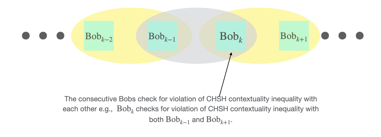
Figure 4: Grouping of consecutive parties in QCP based on CHSH contextuality inequality.

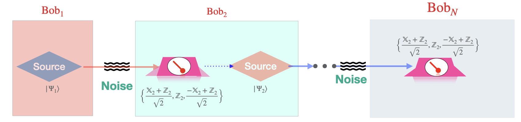
Figure 5: Schematic representation of QCP based on CHSH contextuality inequality.

8.1 Key generation rate

The key generation rate of this protocol is twice that of the Mermin’s contextuality based QCP. The higher key generation rate owes to the fact that the outcomes of two observables per Bob contribute to the key generation whereas, in Mermin-based QCP, the outcome of only one observable per Bob contributes to it. The probability that all the $N$-Bobs choose the same observables is $\frac{1}{3^{N}}$. Since, measurement outcomes of the two sets of observables, i.e., $\{\frac{\mathbb{X}_{1}+\mathbb{Z}_{1}}{\sqrt{2}},\frac{\mathbb{X}_{2}+\mathbb{Z}_{2}}{\sqrt{2}}\};~{}\{\mathbb{Z}_{1},\mathbb{Z}_{2}\}$ are fully correlated, the key generation rate is $\frac{2}{3^{N}}$.

9 Outlook for implementation using OAM states of light

In this section, we examine the feasibility of experimental implementation of the QCPs proposed in sections (6) and (8) using OAM states, although it may not be realised in the immediate future. Depending on the symmetry of laser resonant cavity , Laguerre-Gauss modes Allen , Bessel modesandrews etc., which carry the OAM states of light are experimentally generated. Laguerre-Gauss modes, which are the solutions of paraxial Helmholtz wave equation, have attracted a lot of experimental attentionmode ; mirhosseini ; vaziri ever since they were theoretically proposed Allen . These modes are represented as $LG_{p,l}$, with $p$ being the radial index and $l$, the azimuthal index. The implementation of the protocols employing OAM states requires only linear optics, which makes it realizable with coherent pulses as well. As we are only interested in OAM degree of freedom, we freeze the radial index to be equal to zero, and write the corresponding states as $|LG_{l}\rangle$.

Experimental implementation of the proposed QCPs involve three steps, (i) preparation of the state , (ii) measurement of observables, and (iii) unitary transformations performed on post-measurement state. We outline the implementation of these steps sequentially as follows.

Preparation of state: In Mermin’s contextuality based QCP, we require an initial state, $|\Psi_{M}^{\prime}\rangle$ belonging to a $2^{N}$ dimensional Hilbert space. A state with a definite value of $`l^{\prime}$ or their superposition can be prepared using a spatial light modulator (SLM), which is basically an automated liquid crystal device. So, Mermin-based CQCP can be implemented with single qudit states (e.g., OAM states) whose generation and manipulation are experimentally easier as compared to the multi-party nonlocal states. For example, OAM states with $l_{\rm{max}}=100$ have been prepared with $90\%$ purity Sroor20 , while a four-photon GHZ states have been prepared with $81\%$ purity and $87\%$ fidelity 4photonGHZ . With a $100$ dimensional state, Mermin’s CQCP with only six Bobs can be implemented. However, this limitation no longer exists in the QCP based on CHSH contextuality inequality, which requires only a four-dimensional state irrespective of the number of Bobs involved.
Measurement of observables: The observables in our protocols are dichotomic. Thus, they apportion the Hilbert space into two orthogonal spaces of equal dimensions. Again, SLM can be employed for projecting a state on these eigenprojections.

Unitary transformations: These transformations on OAM states can be performed using beam splitters and Dove prismsleach2004interferometric , or more generically through the programmable holographic techniques Wang17 . This method allows, in principle, the implementation of any unitary transformation on the OAM modes.

Of course, a complete analysis of real-life implementation of these QCPs would also require incorporation of various other effects such as non-ideal behaviour of experimental equipment and turbulence in atmosphere, which has not been considered in this paper.

Finally we note that irrespective of physical system employed for implementation, though we employ $d^{N}$ dimensional quantum states and measurement operators, the key consists of only $d$ symbols.

10 Error analysis

Errors may arise in communication systems due to (i) noisy channels, (ii) imperfections in the preparation of states, (iii) noisy operations, or, (iv) through noisy measurements. In this section, we study the vulnerability of the proposed protocols for imperfect preparation of the state and noisy measurements. We take explicit examples of Mermin and CHSH contextuality-based QCPs. Effect of these errors on the key generation rate is examined. Although masking transformations are required at each step in the protocols, but to make discussion easier, we ignore them for this analysis. We also consider noise only in those states and detectors which are used in the process of key generation, as we are only interested in the effect of these errors on the key generation rate.

Naturally, the asymptotic key generation rate of the protocol is given by the minimum of mutual information when all parties are considered pairwise, i.e.,

$$r=\min_{\begin{subarray}{c}1\leq i,j\leq N\\ i<j\end{subarray}}[I(B_{i},B_{j})],$$ (24)

where $I(B_{i},B_{j})$ is the mutual information between Bob_i and Bob_j.

Please note that the equation (24) falls short of yielding the secret key rate. The effects of various attacks on two–party quantum key distribution protocols have been studied (see scarani2009security and references therein). Extension of those results to the contextuality–based QCPs presented in this work will be taken up separately. The analysis, given in this section, has been restricted to observe the effect of noisy preparation and measurements on the key generation rate.

10.1 Imperfect preparation of the state

10.1.1 Noise in two-dimensional subspace

a) Mermin’s contextuality inequality based QCP :
Recall that the protocol starts with Bob₁ preparing his system in the state $\ket{\Psi_{1}}=\mathbb{\Pi}^{o}_{\mathbb{O}}|\Psi_{M}\rangle$, $\mathbb{O}\in{\cal S}_{1}$. The only measurement that contributes to key generation is that of $\mathbb{Z}_{1}$. Bob₁ wants to prepare either of the states $\ket{0}$ or $\ket{D-1}$ for the respective outcomes $+1$ and $-1$ of the observable $\mathbb{Z}_{1}$. However, as the preparation of the state can be noisy, he would end up preparing either of the following states, given as,

$$\rho_{1M}=(1-\epsilon_{1})\ket{0}\bra{0}+\epsilon_{1}\ket{D-1}\bra{D-1},$$

$$~{}\rho_{2M}=(1-\epsilon_{2})\ket{D-1}\bra{D-1}+\epsilon_{2}\ket{0}\bra{0},$$ (25)

where $\epsilon_{1},~{}\epsilon_{2}$ are small. The effect of this imperfection in the preparation of the state is equivalent to the binary flip channel employed classically, where $\ket{0}$ would flip to $\ket{D-1}$ with probability $\epsilon_{1}$ and $\ket{D-1}$ to $\ket{0}$ with probability $\epsilon_{2}$.

In this QCP, only Bob₁ prepares a state. So, the effect of noise will be prominent in the channel between Bob₁ and Bob₂. The correlation among rest of Bobs is perfect. Therefore, the mutual information between Bob₁ and Bob₂ will be minimum and hence determines the key generation rate, $r_{M}$, i.e.,

$$r_{M}=I(B_{1},B_{2}).$$ (26)

As an illustration, we consider the case of three Bobs and explicitly plot the key rate $(r_{M})$ with respect to $(\epsilon_{1},\epsilon_{2})$ in figure (6).

A similar analysis for QCP based on CHSH contextuality inequality is as follows.
b) CHSH contextuality inequality based QCP :
In this QCP, a key is generated by the measurements of the two sets of observables, $\big{(}\big{\{}\frac{\mathbb{X}_{1}+\mathbb{Z}_{1}}{\sqrt{2}},~{}\frac{\mathbb{X}_{2}+\mathbb{Z}_{2}}{\sqrt{2}}\big{\}};\{\mathbb{Z}_{1},\mathbb{Z}_{2}\}\big{)}$, as explained in section (8). We analyse one set of observables $\{\mathbb{Z}_{1},\mathbb{Z}_{2}\}$. A similar calculation can be done for the other set of observables as well.

Bob₁ prepares either of the states $\ket{1}$ or $\ket{2}$ for the respective outcomes $+1,-1$ of the observable $\mathbb{Z}_{1}$. As the preparation of the states is noisy, he would end up preparing the following states:

$$\rho_{1B}=(1-\epsilon_{1})\ket{1}\bra{1}+\epsilon_{1}\ket{2}\bra{2},$$

$$\rho_{2B}=(1-\epsilon_{2})\ket{2}\bra{2}+\epsilon_{2}\ket{1}\bra{1},$$ (27)

which again admits an analysis via binary flip channel. Recall that in this QCP, each Bob has to prepare the state.

We consider the case of three Bobs. By using equation (24), the key generation rate is given by the minimum of mutual information between any two Bobs, which in this case is $I(B_{1},B_{3})$, i.e.,

$$r_{B}=I(B_{1},B_{3}).$$ (28)

The effect of noisy preparation of states for CQCPs based on both Mermin and CHSH contextuality inequalities can be seen in figures (6) and (7) respectively. The key generation rate falls more rapidly for CQCP based on CHSH inequality. This is a signature of greater noise since both the Bobs (viz., Bob₁ and Bob₂) prepare the state afresh with a noisy apparatus.

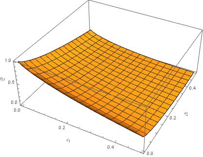
Figure 6: Variation of the key generation rate $r_{M}$ w.r.t noise in the state ($\epsilon_{1},~{}\epsilon_{2}$) for Mermin’s contextuality based QCP for $N=3$. For $\epsilon_{1},~{}\epsilon_{2}=0$, the key generation rate attains its ideal value, i.e., the one in the noiseless scenario.

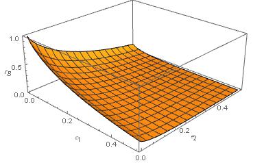
Figure 7: Variation of the key generation rates $r_{B}$ w.r.t noise in the state ($\epsilon_{1},~{}\epsilon_{2}$) for CHSH contextuality based QCP in respectively for $N=3$. For $\epsilon_{1},~{}\epsilon_{2}=0$, the key generation rate attains its ideal value, i.e., the one in the noiseless scenario.

10.1.2 White noise

In this section, we consider a scenario in which the state gets contaminated by the white noise. That is, when Bob₁ wants to prepare the states $\ket{0}\bra{0}$ or $\ket{D-1}\bra{D-1}$, he would instead end up preparing states,

$$\rho^{\prime}_{1} =(1-\epsilon)|0\rangle\langle 0|+\frac{\epsilon}{8}\mathbb{1},$$ (29)

$$\rho^{\prime}_{2} =(1-\epsilon)|D-1\rangle\langle D-1|+\frac{\epsilon}{8}\mathbb{1},$$

respectively. For this kind of noisy preparation, the key generation rate, $r_{2}$, is found to be:

$$r_{2}=I(B_{1},B_{2}),$$ (30)

For the case of three Bobs, the key generation rate is plotted against $\epsilon$ in figure (8). For the sake of comparison, we have also plotted $r_{1}=r_{M}|_{\epsilon_{1},\epsilon_{2}=\epsilon}$ in the same plot.

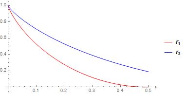
Figure 8: Variation of key generation rates $r_{1}=r_{M}~{}\rm{at}~{}\epsilon_{1},\epsilon_{2}=\epsilon$, and $r_{2}$ w.r.t noise ($\epsilon$) in the state for QCP based on Mermin contextuality inequality.

A similar analysis can be done for QCP based on CHSH contextuality inequality.

10.2 Imperfect detectors

We consider an example of imperfect detectors, that register correctly with a probability $(1-\eta)$ and incorrectly (i.e., in the orthogonal subspace), with a probability $\eta$. Such a detector gets represented by the operator,

$$\mathbb{M}_{\mathbb{Z}_{k}}^{+}=(1-\eta)\mathbb{\Pi}_{\mathbb{Z}_{k}}^{+}+\eta\mathbb{\Pi}_{\mathbb{Z}_{k}}^{-},$$

$$\mathbb{M}_{\mathbb{Z}_{k}}^{-}=\eta\mathbb{\Pi}_{\mathbb{Z}_{k}}^{+}+(1-\eta)\mathbb{\Pi}_{\mathbb{Z}_{k}}^{-};~{}k\in\{2,\cdots,N\}.$$ (31)

The effect of noise in equation (10.2) can be modelled by a binary symmetric channel, endowed with a probability of flip, $\eta.$ In the protocol for three Bobs, since Bob₂ and Bob₃ both perform measurements, the noise can be modelled by two cascaded binary symmetric channels. The key generation rate, $r_{d}$, is found to be,

$$r_{d}=I(B_{2},B_{3}),$$ (32)

which is plotted in figure (9).

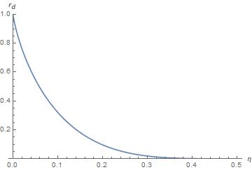
Figure 9: Variation of key generation rate $r_{d}$ w.r.t noise in detector $\eta$.

A similar analysis can be done for CHSH contextuality based QCP.

10.3 Both detectors and states noisy

10.3.1 Model I

Mermin’s contextuality based QCP
Consider a case in which both the state and the measurements are noisy. The noisy measurement is such that it misreads the signal for one projection operator as the other. That is to say, for some fraction of times, it reads $\mathbb{\Pi}^{+}$ as $\mathbb{\Pi}^{-}$ and vice versa. The noisy state sent by Bob₁ to Bob₂ for $+1$ or $-1$ outcome of $\mathbb{Z}_{1}$ respectively are

$$\rho_{1M}=(1-\epsilon_{1})|0\rangle\bra{0}+\epsilon_{1}|D-1\rangle\bra{D-1},$$

$$\rho_{2M}=(1-\epsilon_{2})|D-1\rangle\bra{D-1}+\epsilon_{2}|0\rangle\bra{0}.$$

The noisy measurement operators are:

$$\mathbb{M}_{\mathbb{Z}_{k}}^{+}=(1-\eta)\mathbb{\Pi}_{\mathbb{Z}_{k}}^{+}+\eta\mathbb{\Pi}_{\mathbb{Z}_{k}}^{-},$$

$$\mathbb{M}_{\mathbb{Z}_{k}}^{-}=\eta\mathbb{\Pi}_{\mathbb{Z}_{k}}^{+}+(1-\eta)\mathbb{\Pi}_{\mathbb{Z}_{k}}^{-};~{}k\in\{2,\cdots,N\}.$$ (33)

Consider a special case of three Bobs. The key generation rate is given by the minimum of pairwise mutual information. For this model, depending upon the amount of noise, we observe the interplay between mutual information between Bob₁ and Bob₂, $I(B_{1},B_{2})$ and mutual information between Bob₂ and Bob₃, $I(B_{2},B_{3})$. The key generation rate $r_{M}$ is found to be

$$r_{M}=\min[I(B_{1},B_{2}),I(B_{2},B_{3})].$$ (34)

We have plotted this key generation rate $r_{M}$ for a fixed $\eta=0.1$ (noise in the detector) w.r.t noise in the preparation of state, ($\epsilon_{1},~{}\epsilon_{2}$), in figure (10). The left side of discontinuity in the figure represent the region over which $I(B_{2},B_{3})$ is minimum and on the right side $I(B_{1},B_{2})$ is minimum.

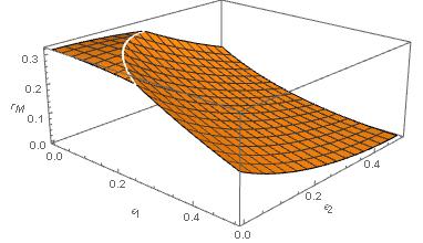
Figure 10: Variation of key generation rate ($r_{M}$) for a particular $\eta=0.1$ (noise in the detector) w.r.t noise in the preparation of state, ($\epsilon_{1},~{}\epsilon_{2}$), for QCP based on Mermin contextuality inequality.

In a similar way, calculation for CHSH contextuality based QCP can be performed.

10.3.2 Model II

Mermin’s contextuality based QCP
In this model, we consider an imperfect preparation of the state and lossy detectors. The detector misses a signal with a probability $(1-\eta)$ and is represented as:

$$\mathbb{M}_{\mathbb{Z}}^{\pm}=\eta\mathbb{\Pi}_{\mathbb{Z}}^{\pm}.$$ (35)

Consider a particular case of three Bobs, for which Bob₁ prepares the two states with an equal probability:

$$\rho_{1}=(1-\epsilon_{1})|0\rangle\bra{0}+\epsilon_{1}|7\rangle\bra{7},$$

$$\rho_{2}=(1-\epsilon_{2})|7\rangle\bra{7}+\epsilon_{2}|0\rangle\bra{0}.$$ (36)

The effect of this channel on the protocol can be modelled by binary flip channel and erasure channel. The minimum mutual information is found to be $I(B_{1},B_{3})$ and hence act as the key generation rate, $r_{M}$, i.e.,

$$r_{M}=I(B_{1},B_{3}).$$ (37)

A similar analysis can be done for CHSH contextuality based QCP for which the key generation rate, $r_{B}$, is found to be:

$$r_{B}=I(B_{1},B_{3}).$$ (38)

Effect of this noisy channel on the key generation rate is plotted in figures (11) and (12) for QCP based on Mermin and CHSH contextuality inequality respectively.

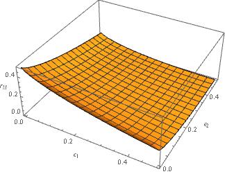
Figure 11: Variation of the key generation rate $r_{M}$ w.r.t noise in the state ($\epsilon_{1}$ and $\epsilon_{2}$) for model II for $\eta=0.7$ noise in detector for QCP based on Mermin contextuality inequality.

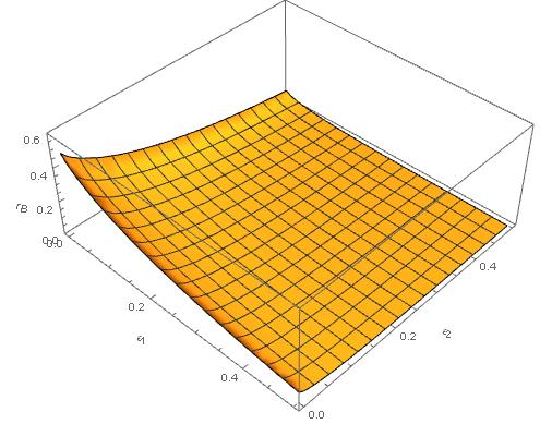
Figure 12: Variation of the key generation rate $r_{B}$ w.r.t noise in the state ($\epsilon_{1}$ and $\epsilon_{2}$) for model II for $\eta=0.7$ noise in detector for QCP based on CHSH contextuality inequality.

11 Conclusion

In summary, we have laid down the procedure to obtain device-dependent CQCP from any NQCP. These protocols do not involve multiparty nonlocal states. Two classes of QCPs are proposed through the examples of Mermin’s and CHSH contextuality inequality. The latter is more beneficial as it alleviates the constraint on the number of Bobs who can participate in the key sharing process.

Finally, the equivalence of multi-party nonlocality and single qudit contextuality which we have shown here, can be used to develop contextuality-based quantum secure direct communication protocols from nonlocality-based quantum secure direct communication protocols.

Author Contribution Statement

All the authors contributed equally in all respects.

Appendix A Mermin’s nonlocality inequality as contextuality inequality

The interrelation between the two-party nonlocality and single-qudit contextuality, shown in the section (3.1) for CHSH inequality, continues to hold even for multi-party nonlocality inequalities. We illustrate it through the example of Mermin’s inequality. For that, we briefly recapitulate Mermin’s inequality for an $N$-party system.

Mermin’s inequality distinguishes the states admitting completely factorisable local hidden variable model from nonlocal states.

Consider a pair of dichotomic observables $\{A_{j},A^{\prime}_{j}\}$ in the space of the $j^{\rm th}$ party ($j\in\{1,\cdots,N\}$). The inequality is as follows Mermin90 :

$${\cal M}_{N} =\frac{1}{2i}\Bigg{|}\bigg{\langle}\prod_{j=1}^{N}(A_{j}+iA^{\prime}_{j})-\prod_{j=1}^{N}(A_{j}-iA^{\prime}_{j})\bigg{\rangle}\Bigg{|}\leq c$$

$$c =2^{N/2},\quad N={\rm even},$$ (39)

$$=2^{\frac{N-1}{2}},\quad N={\rm odd};N\geq 3.$$

The observables corresponding to different parties commute and $[A_{k},A^{\prime}_{k}]\neq 0$.

For the special case of an $N$ qubit system, the inequality (A) gets maximally violated by the GHZ state,

$$|\phi_{N}\rangle=\dfrac{1}{\sqrt{2}}\bigg{(}|0\rangle^{\otimes N}+i|1\rangle^{\otimes N}\bigg{)},$$ (40)

for the following choice of the observables:

$$A_{k}=X_{k};~{}A^{\prime}_{k}=Y_{k}.$$ (41)

It is pertinent to illustrate the contextual behaviour of $|\phi_{N}\rangle$ to substantiate our claim. For that purpose, we consider the following two contexts:
Context 1 ($Z_{1}Z_{2}\cdots Z_{N-1}Z_{N}$): Suppose the outcome of $Z_{1}$ is $+1(-1)$. Then, the outcomes of observables $Z_{2},Z_{3},\cdots,Z_{N}$ will be $+1(-1)$ with unit probability.
Context 2 ($Y_{1}Z_{2}\cdots Z_{N}$): Let the outcome of the measurement of $Y_{1}$ be once again, +1. Following it, the measurement of observable $Z_{2}$ will yield $+1$ or $-1$ with equal probability. Thereafter, the measurement of $Z_{3},\cdots,Z_{N}$ will definitely yield +1. Thus, the outcome of $Z_{2}$ depends on the set of commuting observables it is measured with, i.e., it depends on the context.
Exactly in the same manner as in the section (3.1), the observables and the state in the $2^{N}$ dimensional Hilbert space can be identified.

$$|\phi_{N}\rangle\mapsto|\Phi\rangle=\dfrac{1}{\sqrt{2}}(|0\rangle+i|2^{N}-1\rangle)$$ (42)

The equivalent observables $\{\mathbb{Z}_{1},\cdots,\mathbb{Z}_{N},\mathbb{Y}_{1}\}$ can be obtained by following the prescription in point (2) and (3) of section (2), and they satisfy the same commutation relations as $\{{Z}_{1},\cdots,{Z}_{N},{Y}_{1}\}$ because of operator isomorphism.
Thus, Mermin’s inequality probes contextuality in a qudit of appropriate higher dimension and can be referred to as Mermin’s contextuality inequality.

Appendix B Illustration of eavesdropping

To illustrate the point that how Eve obtains information about the key without disturbing the violation of contextuality inequality, we consider the QCP based on Mermin’s contextuality inequality. Consider an example of three parties, Bob₁, Bob₂ and Bob₃. We choose following set of observables:

$$\mathbb{Z}_{1}=\ket{0}\bra{0}+\ket{1}\bra{1}+\ket{2}\bra{2}+\ket{3}\bra{3}$$

$$~{}~{}~{}~{}~{}-\Big{(}\ket{4}\bra{4}+\ket{5}\bra{5}+\ket{6}\bra{6}+\ket{7}\bra{7}\Big{)}$$

$$\mathbb{Z}_{2}=\ket{0}\bra{0}+\ket{1}\bra{1}+\ket{4}\bra{4}+\ket{5}\bra{5}$$

$$~{}~{}~{}~{}~{}-\Big{(}\ket{2}\bra{2}+\ket{3}\bra{3}+\ket{6}\bra{6}+\ket{7}\bra{7}\Big{)}$$

$$\mathbb{Z}_{3}=\ket{0}\bra{0}+\ket{2}\bra{2}+\ket{4}\bra{4}+\ket{6}\bra{6}$$

$$~{}~{}~{}~{}~{}~{}-\Big{(}\ket{1}\bra{1}+\ket{3}\bra{3}+\ket{5}\bra{5}+\ket{7}\bra{7}\Big{)}$$

$$\mathbb{X}_{1}=\ket{0^{+}}\bra{0^{+}}+\ket{1^{+}}\bra{1^{+}}+\ket{2^{+}}\bra{2^{+}}+\ket{3^{+}}\bra{3^{+}}$$

$$~{}~{}~{}~{}~{}-\Big{(}\ket{0^{-}}\bra{0^{-}}+\ket{1^{-}}\bra{1^{-}}+\ket{2^{-}}\bra{2^{-}}+\ket{3^{-}}\bra{3^{-}}\Big{)},$$ (43)

where the symbols $\ket{l^{\pm}}$ are defined as,

$$\ket{l^{\pm}}=\frac{1}{\sqrt{2}}(\ket{l}\pm\ket{l+4});~{}~{}~{}l\in\{0,1,2,3\}$$ (44)

Consider the following two situations, one in which there is no eavesdropping, the other in which Eve is present.

1. Case I: Following the steps of Mermin’s contextuality based QCP, let Bob₁ prepares a state $\ket{\Psi_{M}^{\prime}}=\ket{0}$ for the +1 outcome of $\mathbb{Z}_{1}$ on the reference state $\ket{\Psi_{M}}$. He sends this state $\ket{\Psi_{M}^{\prime}}$ to Bob₂. If Bob₂ measures, say, $\mathbb{Z}_{2}$ on this state, he obtains the outcome +1 with unit probability. Thereafter, he sends the post-measurement state to Bob₃. Bob₃ measures, say, $\mathbb{Z}_{3}$, he is bound to get outcome +1 with unit probability.

2. Case II: Let there be an eavesdropping between Bob₂ and Bob₃. Eve measures an observable, $\mathbb{X_{1}}$. She obtains $\pm 1$ with equal probability and the state collapses to $\ket{\Phi^{\pm}}=\frac{1}{\sqrt{2}}(\ket{0}\pm\ket{4})$. She sends the post-measurement state to Bob₃. Bob₃ measures an observable $\mathbb{Z}_{3}$, as in the previous case, and obtains outcome +1 with unit probability.
   Thus, the measurement of Eve does not affect the outcome of Bob₃’s measurement. Due to this, Bob₃ will never detect presence of Eve. In this way, Eve can obtain full information about the key by choosing appropriate observable without being detected.

References

- [1] Lov K. Grover. Quantum mechanics helps in searching for a needle in a haystack. Phys. Rev. Lett., 79:325–328, 1997.
- [2] David Deutsch and Richard Jozsa. Rapid solution of problems by quantum computation. Proc. Math. Phys. Eng. Sci., 439(1907):553–558, 1992.
- [3] Charles H. Bennett and Stephen J. Wiesner. Communication via one- and two-particle operators on einstein-podolsky-rosen states. Phys. Rev. Lett., 69:2881–2884, 1992.
- [4] Charles H. Bennett, Gilles Brassard, Claude Crépeau, Richard Jozsa, Asher Peres, and William K. Wootters. Teleporting an unknown quantum state via dual classical and einstein-podolsky-rosen channels. Phys. Rev. Lett., 70:1895–1899, 1993.
- [5] C. Bennett and G. Brassard. Quantum cryptography: public key distribution and coin tossing. Proc. IEEE Int. Conf. on Comp. Sys. Signal Process (ICCSSP), page 175, 1984.
- [6] Artur K. Ekert. Quantum cryptography based on bell’s theorem. Phys. Rev. Lett., 67:661–663, Aug 1991.
- [7] Min Namkung and Younghun Kwon. Generalized sequential state discrimination for multiparty qkd and its optical implementation. Scientific Reports, 10(1):1–35, 2020.
- [8] William K Wootters and Wojciech H Zurek. A single quantum cannot be cloned. Nature, 299(5886):802–803, 1982.
- [9] Umesh Vazirani and Thomas Vidick. Fully device-independent quantum key distribution. Phys. Rev. Lett., 113:140501, Sep 2014.
- [10] Xiaolong Su. Applying gaussian quantum discord to quantum key distribution. Chinese science bulletin, 59(11):1083–1090, 2014.
- [11] Stefano Pirandola. Quantum discord as a resource for quantum cryptography. Scientific reports, 4:6956, 2014.
- [12] J. E. Troupe and J. M. Farinholt. A contextuality based quantum key distribution protocol. arxiv, 2015.
- [13] Jaskaran Singh, Kishor Bharti, and Arvind. Quantum key distribution protocol based on contextuality monogamy. Phys. Rev. A, 95:062333, Jun 2017.
- [14] Koji Nagata. Kochen-specker theorem as a precondition for secure quantum key distribution. Phys. Rev. A, 72:012325, 2005.
- [15] Peter Heywood and Michael LG Redhead. Nonlocality and the kochen-specker paradox. Foundations of physics, 13(5):481–499, 1983.
- [16] N. David Mermin. Simple unified form for the major no-hidden-variables theorems. Phys. Rev. Lett., 65:3373–3376, Dec 1990.
- [17] Otfried Gühne, Matthias Kleinmann, Adán Cabello, Jan-Åke Larsson, Gerhard Kirchmair, Florian Zähringer, Rene Gerritsma, and Christian F. Roos. Compatibility and noncontextuality for sequential measurements. Phys. Rev. A, 81:022121, Feb 2010.
- [18] Samson Abramsky and Adam Brandenburger. The sheaf-theoretic structure of non-locality and contextuality. New Journal of Physics, 13(11):113036, 2011.
- [19] MW Beijersbergen, RPC Coerwinkel, M Kristensen, and JP Woerdman. Helical-wavefront laser beams produced with a spiral phaseplate. Optics communications, 112(5-6):321–327, 1994.
- [20] N. R. Heckenberg, R. McDuff, C. P. Smith, and A. G. White. Generation of optical phase singularities by computer-generated holograms. Opt. Lett., 17(3):221–223, Feb 1992.
- [21] A. Mair, A. Vaziri, G. Weihs, and A. Zeilinger. Entanglement of the orbital angular momentum states of photons. Nature, 412:313, 2001.
- [22] Jonathan Leach, Miles J Padgett, Stephen M Barnett, Sonja Franke-Arnold, and Johannes Courtial. Measuring the orbital angular momentum of a single photon. Physical review letters, 88(25):257901, 2002.
- [23] Gregorius CG Berkhout, Martin PJ Lavery, Johannes Courtial, Marco W Beijersbergen, and Miles J Padgett. Efficient sorting of orbital angular momentum states of light. Physical review letters, 105(15):153601, 2010.
- [24] A.C. Dada et al. Experimental high-dimensional two-photon entanglement and violations of generalized bell inequalities. Nature Physics, 7:677, Apr 2011.
- [25] R. Fickler, R. Lapkiewicz, W. Plick, C. Krenn, M.m Schaeff, S. Ramelow, and A. Zeilinger. Quantum entanglement of high angular momenta. Science, 338:640, 2012.
- [26] Mehul Malik, Mohammad Mirhosseini, Martin PJ Lavery, Jonathan Leach, Miles J Padgett, and Robert W Boyd. Direct measurement of a 27-dimensional orbital-angular-momentum state vector. Nature communications, 5(1):1–7, 2014.
- [27] Zhi-Yuan Zhou, Yan Li, Dong-Sheng Ding, Wei Zhang, Shuai Shi, Bao-Sen Shi, and Guang-Can Guo. Orbital angular momentum photonic quantum interface. Light: Science & Applications, 5(1):e16019–e16019, 2016.
- [28] Juan Yin, Yuan Cao, Yu-Huai Li, Sheng-Kai Liao, Liang Zhang, Ji-Gang Ren, Wen-Qi Cai, Wei-Yue Liu, Bo Li, Hui Dai, et al. Satellite-based entanglement distribution over 1200 kilometers. Science, 356(6343):1140–1144, 2017.
- [29] Manuel Erhard, Robert Fickler, Mario Krenn, and Anton Zeilinger. Twisted photons: new quantum perspectives in high dimensions. Light: Science & Applications, 7(3):17146–17146, 2018.
- [30] J. F. Clauser, M. A. Horne, A. Shimony, and R. A. Holt. Proposed experiment to test local hidden-variable theories. Phys. Rev. Lett., 23(15):880, October 1969.
- [31] Nicolas Brunner, Daniel Cavalcanti, Stefano Pironio, Valerio Scarani, and Stephanie Wehner. Bell nonlocality. Rev. Mod. Phys., 86:419–478, Apr 2014.
- [32] Yonggi Jo and Wonmin Son. Semi-device-independent multiparty quantum key distribution in the asymptotic limit. OSA Continuum, 2(3):814–826, 2019.
- [33] L. Allen, M. W. Beijersbergen, R. J. C. Spreeuw, and J. P. Woerdman. Orbital angular momentum of light and the transformation of laguerre-gaussian laser modes. Phys. Rev. A, 45:8185–8189, Jun 1992.
- [34] Les Allen and Miles Padgett. Chapter 1 - introduction to phase-structured electromagnetic waves. In DAVID L. ANDREWS, editor, Structured Light and Its Applications, pages 1 – 17. Academic Press, Burlington, 2008.
- [35] Anna T O’Neil and Johannes Courtial. Mode transformations in terms of the constituent hermite–gaussian or laguerre–gaussian modes and the variable-phase mode converter. Optics communications, 181(1-3):35–45, 2000.
- [36] Mohammad Mirhosseini, Mehul Malik, Zhimin Shi, and Robert W Boyd. Efficient separation of the orbital angular momentum eigenstates of light. Nature communications, 4(1):1–6, 2013.
- [37] Alipasha Vaziri, Gregor Weihs, and Anton Zeilinger. Superpositions of the orbital angular momentum for applications in quantum experiments. Journal of Optics B: Quantum and Semiclassical Optics, 4(2):S47, 2002.
- [38] Hend Sroor, Yao-Wei Huang, Bereneice Sephton, Darryl Naidoo, Adam Vallés, Vincent Ginis, Cheng-Wei Qiu, Antonio Ambrosio, Federico Capasso, and Andrew Forbes. High-purity orbital angular momentum states from a visible metasurface laser. Nature Photonics, pages 1–6, 2020.
- [39] Massimiliano Proietti, Joseph Ho, Federico Grasselli, Peter Barrow, Mehul Malik, and Alessandro Fedrizzi. Experimental quantum conference key agreement. Science Advances, 7(23):eabe0395, 2021.
- [40] Jonathan Leach, Johannes Courtial, Kenneth Skeldon, Stephen M Barnett, Sonja Franke-Arnold, and Miles J Padgett. Interferometric methods to measure orbital and spin, or the total angular momentum of a single photon. Physical review letters, 92(1):013601, 2004.
- [41] Yu Wang, Václav Potoček, Stephen M. Barnett, and Xue Feng. Programmable holographic technique for implementing unitary and nonunitary transformations. Phys. Rev. A, 95:033827, Mar 2017.
- [42] Valerio Scarani, Helle Bechmann-Pasquinucci, Nicolas J Cerf, Miloslav Dušek, Norbert Lütkenhaus, and Momtchil Peev. The security of practical quantum key distribution. Reviews of modern physics, 81(3):1301, 2009.
- [43] N. David Mermin. Extreme quantum entanglement in a superposition of macroscopically distinct states. Phys. Rev. Lett., 65:1838–1840, 1990.