Discerning Signatures of Seesaw Models and Complementarity of Leptonic Colliders

Abstract

The seesaw extensions of the Standard Models are well motivated in explaining the tiny neutrino mass. In the process these models predict extra heavy Majorana neutrino, charged lepton and charged scalars depending on the scenarios. Distinguishing such scenarios at the colliders would be one of the first goals if we receive some hint of those. We show how various leptonic colliders can play a role of complementarity in segregating such scenarios and the angular distributions can be instrumental, which carry the information of the matrix element. The $\ell^{-}\,\ell^{-},\ell^{+}\,\ell^{-}\,\ell^{\prime\,+}\ell^{-}$ colliders are explored in investigating such possibility via a PYTHIA based simulation. We emphasis on muon collider and comment on the prospect of $\mu\,e$ collider as well.

1 Introduction

During last few decades Standard Model (SM) has established its supremacy over all the other contemporary models. However, the outcomes from several experiments insinuate that it does not provide a complete theoretical description for all the elementary particles. One of the areas to seek for such beyond Standard Model (BSM) effects is the neutrino sector Bilenky:1987ty . While the SM considers neutrinos to be massless, left-chiral, Weyl fermions interacting through the EW processes only, neutrino oscillation data Zyla:2020zbs , evinces their massive nature, though tiny. Therefore, they should be either Dirac fermions or Majorana fermions by nature. Nevertheless, any irrefutable signature advocating the presence of right-chiral neutrinos in nature has not been found yet. The seesaw models, where a few number of heavy BSM particles are introduced along with the SM ones, are very elegant in resolving this issue in a ingenious way. To address this problem, while heavy right-handed singlet and triplet fermions are introduced in case of Type-I and Type-III seesaw respectively, Type-II scenario considers very massive additional scalars, triplet under $SU(2)$. Again, there exist inverse seesaw mechanisms, where two sets of the light lepton flavor violating singlet or the triplet fermions with heavy mixing among the flavour eigenstates are presumed. But the price paid in all of these scenarios is that the mass eigenstates of neutrinos become Majorana fermions. Possibilities of separating these different seesaw models at the colliders like the LHC has already been studied widely Bajc:2007zf ; delAguila:2008cj ; Deppisch:2015qwa ; Cai:2017mow ; FileviezPerez:2008jbu ; Melfo:2011nx ; Franceschini:2008pz ; Li:2009mw ; Aguilar-Saavedra:2013twa ; Bandyopadhyay:2011aa ; ATLAS:2020wop ; CMS:2017ybg ; CMS:2019lwf ; Goswami:2017jqs ; Das:2012ze ; Das:2018usr ; Das:2020gnt ; Bandyopadhyay:2012px ; Bandyopadhyay:2014sma ; Bandyopadhyay:2011qm ; Bandyopadhyay:2015iij ; Atre:2009rg . But the viability of any of these seesaw models has yet to be verified experimentally.

Though the hadronic colliders have the advantage of reaching very high centre of mass energy, the hadronically unclean environment makes it difficult to identify the signal with high significance. This motivates us to look into leptonic colliders, where hadronic backgrounds are small in number or negligible. In this paper, we have investigated the distinctive features of several seesaw models at various leptonic colliders. Different $\ell^{+}\ell^{-}$ machines ($\ell$ denotes muon or electron) with high energy and luminosity like ILC, CLIC, FCC-ee, muon colliders are going to be build in near feature. There is also an upcoming project MUoNE which aims to measure the hadronic contribution to muon $g-2$ through thee elastic $\mu e$ scattering. Again, there is proposal of $\ell^{-}\ell^{-}$ collider Heusch:1997fn ; Arkani-Hamed:1996bxi ; Feng:1996fg ; Feng:1999zv ; DeRoeck:2003cjp ; Heusch:2005iy ; Rodejohann:2010bv also which has not been built so far because of very limited attainable SM finalstates at these colliders. For instance, the only $2\to 2$ process possible at $e^{-}e^{-}$ collider under SM is the Møller scattering. Notwithstanding, this exquisite idiosyncrasy of $e^{-}e^{-}$ collision can now be used as a tool to keep the signal very clean while hunting for minuscule traces of BSM Physics, generally imperceptible.

It has been noticed that the angular distribution acts as a great tool in separating various BSM scenarios Datta:2005zs ; Battaglia:2005ma ; Christensen:2013aua ; Bandyopadhyay:2020jez ; Bandyopadhyay:2020klr ; Bandyopadhyay:2020wfv . In this article we have used this tool to separate all the seesaw models at leptonic colliders. We choose several benchmark points in accordance with current experimental bounds along with diagonal coupling and study the possibility of discerning different seesaw scenarios using the angular distributions. Since, the consideration of the neutrino masses compels the Yukawa coupling for the TeV scaled BSM particles to be very small for both Type-I and Type-III cases, it is very challenging to detect their trace at any collider. Therefore, we use inverse Type-I and Type-III seesaw models, where the smallness of active neutrino masses is controlled by an additional parameter $\mu_{n}$. For each of the models considered, we select different finalstate and eventually look at the angular distribution of the finalstate leptons or the reconstructed BSM particle in the CM frame with respect to its angle with the beam axis. We find very distinctive angular distributions for different seesaw models at individual leptonic collider.

The paper is organized in following way. In the next section, we briefly discuss the theoretical description of different seesaw models while in section 3 we present the importance of angular distribution in discerning different BSM cases. section 4 goes over the setup for collider simulation. The subsequent section (section 5) deals with differentiating seesaw models at $\ell^{-}\ell^{-}$ collider. In section 6 we scrutinize the possibility of the same at $\ell^{+}\ell^{-}$ collider. The following section (section 7) discusses the prospect of $\ell^{+}\ell^{\prime-}$ collider in this regard. Finally, we conclude in section 8.

2 Different seesaw models

In this section, we brief about different seesaw scenarios and the BSM particle spectrum that we look for at the future colliders.

2.1 Type-I seesaw

In case of Type-I seesaw Minkowski:1977sc ; Yanagida:1979as ; Gell-Mann:1979vob ; Glashow:1979nm ; PhysRevLett.44.912 , three generations of $SU(2)_{L}$ singlet, colourless, heavily massive right-handed neutrinos $(N_{R}\,(\bm{1,1},0))$ with zero hypercharge are introduced which have the relevant interactions and mass terms in the Lagrangian as follows:

$$-\mathscr{L}_{I}\supset Y_{\nu}\,\hbox{\vbox{\hrule height=0.65pt\kern 1.72218pt\hbox{\kern-0.50003pt$L$\kern 0.0pt}}}\,\widetilde{H}N_{R}+\frac{1}{2}M_{R}\,\hbox{\vbox{\hrule height=0.65pt\kern 1.72218pt\hbox{\kern-0.50003pt$N^{\,c}_{R}$\kern 0.0pt}}}\,N_{R}\,+h.c.\,,$$ (1)

where, $L$ and $H\big{(}\equiv(H^{+},H^{0})^{T}\big{)}$ are lepton and Higgs doublets in SM with $\widetilde{H}=i\sigma_{2}H^{*}$, $Y_{\nu}$ and $M_{R}$ are coupling and mass matrices with generation indices being suppressed. Here, the notation used for charge conjugate field is: $\psi^{c}_{L,R}\equiv(\psi_{L,R})^{c}$. After the electroweak symmetry breaking (EWSB) the SM neutrinos and the Majorana fermion $N_{R}^{c}$ mix, leaving one set of light and another set of heavy neutrinos. The mass-matrix in the flavour basis and the masses for light ($\nu$) and heavy ($N^{0}$) neutrinos are given by:

$$\begin{split}\mathcal{M}=\begin{pmatrix}0&\frac{v_{0}}{\sqrt{2}}Y_{\nu}\\ \frac{v_{0}}{\sqrt{2}}Y_{\nu}^{T}&M_{R}\end{pmatrix},{}&\quad m_{\nu}\approx\,\frac{v_{0}^{2}}{2}\,Y_{\nu}M_{R}^{-1}\,Y_{\nu}^{T}\\ \text{and}{}&\quad M_{N^{0}}\approx M_{R},\end{split}$$ (2)

(assuming $|v_{0}Y_{\nu}/\sqrt{2}|\ll|M_{R}|$) with $H$ becoming $(0,h+v_{0})^{T}/\sqrt{2}$ under unitary gauge, where the vev of $H$ is $v_{0}/\sqrt{2}$. After the production, each of these heavy neutrinos will decay through $Z\nu$, $h\nu$ and $W^{\pm}l^{\mp}$ modes with the decay widths given by:

$$\Gamma^{Z\nu}_{N^{0}}\approx\Gamma^{h\nu}_{N^{0}}\approx\frac{1}{2}\Gamma^{Wl}_{N^{0}}\approx\frac{Y_{\nu}^{2}M_{R}}{32\pi}\leavevmode\nobreak\ .$$ (3)

But, it is apparent from Equation 2 that the neutrino mass of $\mathcal{O}\,(10^{-1}\,\text{eV})$ either restricts the couplings of the SM leptons with the TeV-scaled BSM particles to be $\mathcal{O}\,(10^{-6})$ or compels the new particles to be heavier than $10^{5}$ TeV for the coupling higher than $10^{-3}$. This makes the signatures of usual Type-I seesaw models very difficult to be observed even at the future experimental facilities. Notwithstanding, the inverse seesaw (ISS) kind of scenarios has the prospect to be within the detectable limit of future experiments. For Type-I case Mohapatra:1986aw ; Nandi:1985uh ; PhysRevD.34.1642 , one introduces three generations of two right-handed singlet neutrino fields $(N_{a},\,N_{b})$, only one $(N_{a})$ of which couples to SM leptons. In this case, though the flavour states are very light, there exists a large off-diagonal coupling between $N_{a}$ and $N_{b}$ through the mass term $M_{n}$. The mass and Yukawa terms of the Lagrangian for this case is given by:

$$-\mathscr{L}_{I}^{in}=Y\,\hbox{\vbox{\hrule height=0.65pt\kern 1.72218pt\hbox{\kern-0.50003pt$L$\kern 0.0pt}}}\,\widetilde{H}\,N_{a}+M_{n}\,\hbox{\vbox{\hrule height=0.65pt\kern 1.72218pt\hbox{\kern-0.50003pt$N_{a}^{\,c}$\kern 0.0pt}}}\,N_{b}+\frac{1}{2}\,\mu_{n}\hbox{\vbox{\hrule height=0.65pt\kern 1.72218pt\hbox{\kern-0.50003pt$N_{b}^{\,c}$\kern 0.0pt}}}\,N_{b}\,+h.c.,$$ (4)

where the generation indices have been suppressed. Here, $Y$ is the Yukawa coupling of $N_{a}$ with SM leptons, large mass term $M_{n}$ indicates the mixing between $N_{a}$ and $N_{b}$, whereas, the tiny mass term $\mu_{n}$ (in general a complex symmetric matrix) signify the mass of $N_{b}$. After EWSB and the mixing of the flavour states, there emerges one set of light neutrinos ($\nu$) and two sets of heavy neutrinos ($N^{0},\widetilde{N}^{0}$), each set consisting of three generations. The entire mass matrix in the flavour basis along with masses for light and heavy neutrinos here can be expressed as:

$$\begin{split}\mathcal{M}{}&=\begin{pmatrix}0&\frac{v_{0}}{\sqrt{2}}Y&0\\ \frac{v_{0}}{\sqrt{2}}Y^{T}&0&M_{n}\\ 0&M_{n}^{T}&\mu_{n}\end{pmatrix},\\ m_{\nu}\approx\frac{v_{0}^{2}}{2}\,Y(M_{n}^{-1})^{T}{}&\mu_{n}\,M_{n}^{-1}Y^{T},\quad M_{N^{0}}^{2}\approx M_{\widetilde{N}^{0}}^{2}\approx M_{n}\,M_{n}^{T}\,,\end{split}$$ (5)

where it has been assumed that $|v_{0}Y/\sqrt{2}|\ll|M_{n}|$. As can be noticed from above equation, apart from the Yukawa coupling $Y$ and the large mass $M_{n}$, the smallness of active neutrino mass matrix in this case is controlled by an additional parameter $\mu_{n}$. Hence, with the suitable choice of $\mu_{n}$, the coupling s$Y$ could be $\mathcal{O}\,(10^{-1})$ for $M_{n}\sim\mathcal{O}(1$ TeV), which makes this testable at present and future colliders.

The heavy leptons will finally decay to light leptons associated with Higgs boson or weak gauge bosons. The partial decay widths for each generation of $N^{0}$ and $\widetilde{N}^{0}$ in different channels are given by:

$$\Gamma^{Z\nu}_{N^{0}/\widetilde{N}^{0}}\approx\Gamma^{h\nu}_{N^{0}/\widetilde{N}^{0}}\approx\frac{1}{2}\Gamma^{Wl}_{N^{0}/\widetilde{N}^{0}}\approx\frac{Y^{2}M_{n}}{64\pi}\leavevmode\nobreak\ .$$ (6)

It is interesting to notice that the partial decay width for each channel presented in Equation 3 is twice of that in Equation 6. This fact can easily be understood by investigating the $h\nu$ mode. The scalar field $H$ couples to the right handed neutrinos through the $Y\,\hbox{\vbox{\hrule height=0.65pt\kern 1.72218pt\hbox{\kern-0.50003pt$L$\kern 0.0pt}}}\,\widetilde{H}\,N_{a}$, where only $N_{a}$ field contributes. Now, $N_{a}$ contains $\sim 50\%$ of $N_{0}$ as well as $\sim 50\%$ of $\widetilde{N}_{0}$ unlike the usual Type-I seesaw, where $N_{0}$ is $\sim 100\%$ of $N_{R}$. Similar thing happens for other decay channels also.

2.2 Type-II seesaw

For Type-II seesaw Konetschny:1977bn ; PhysRevD.22.2227 ; Magg:1980ut ; Cheng:1980qt ; Lazarides:1980nt ; Mohapatra:1980yp ; Wetterich:1981bx ; Gelmini:1980re ; Chun:2013vma , a colourless $SU(2)_{L}$ triplet (adjoint) scalar $(\Delta\,(\bm{1,3},1))$ with hypercharge one, mass $M_{\Delta}$, coupling with Higgs as $\mu_{\Delta}$ and Yukawa coupling $Y_{\Delta}$ is added to particle list. The pertinent portion of Lagrangian is given by:

$$\begin{split}-\mathscr{L}_{II}{}&\supset M_{\Delta}^{2}\,Tr\,(\Delta^{\dagger}\Delta)+\Big{[}Y_{\Delta}\,\hbox{\vbox{\hrule height=0.65pt\kern 1.54996pt\hbox{\kern-0.45003pt$L$\kern 0.0pt}}}^{\,c}(i\sigma_{2}\,\Delta^{\dagger})\,L-\mu_{\Delta}\,\widetilde{H}^{\dagger}\Delta^{\dagger}H+h.c.\Big{]}\\ {}&\text{with}\quad\Delta=\begin{pmatrix}\Delta^{+}/\sqrt{2}&\Delta^{++}\\ \Delta^{0}&-\Delta^{+}/\sqrt{2}\end{pmatrix}.\end{split}$$ (7)

Though, there could be other gauge invariant terms in the Lagrangian involving quartic couplings of triplet and the SM doublet as well as the self-quartic coupling of the triplet, for our analysis these terms remain irrelevant and hence we do not write them down explicitly. After the symmetry breaking, the neutral component of $\Delta$ acquires a small vev of $v_{\Delta}/\sqrt{2}$ and consequently, the neutrinos pick up a Majorana mass term in the following form:

$$m_{\nu}=\sqrt{2}\,v_{\Delta}\,Y_{\Delta}\quad\text{where}\quad v_{\Delta}\approx\frac{\mu_{\Delta}v_{0}^{2}}{\sqrt{2}\,M_{\Delta}^{2}}\,.$$ (8)

Now, the doubly charged scalar can decay to same sign di-lepton (SSD) or di-boson channels. While the decay width to di-lepton channel is proportional to $Y_{\Delta}^{2}$, the same to di-boson mode varies as $v_{\Delta}^{2}$.

         

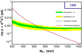
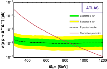
Figure 1: (a) CMS CMS:2017pet and (b) ATLAS ATLAS:2017xqs bounds on the Type-II scalers. The black dashed lines are the expected medians, whereas, the green and yellow bands present the $1\sigma$ and $2\sigma$ regions, respectively. The red line represents the theoretical prediction for the associate production and pair production of Type-II scalers for CMS and ATLAS, respectively.

As can be noticed from the above equation that the coupling $Y_{\Delta}$ can take the value $\mathcal{O}\,(10^{-1})$ for a TeV scaled scalar triplet with $\mu_{\Delta}\sim 20$ eV satisfying $m_{\nu}\sim 0.1$ eV, accordingly creating the possibility to probe it in experiments.

The $\rho$ parameter in this model can be expressed as:

$$\rho=\frac{1+(2v_{\Delta}^{2}/v_{0}^{2})}{1+(4v_{\Delta}^{2}/v_{0}^{2})}\leavevmode\nobreak\ ,$$ (9)

which in accordance with the present electroweak precision measurement of $\rho=1.00037\pm 0.00023$ pdg indicates that $v_{\Delta}\leq 2.1$ GeV. Type-II seesaw model can contribute to lepton flavour violating decays $\tau\to\bar{\ell}_{j}\ell_{k}\ell_{m}$ or $\mu\to\bar{e}ee$ at tree level via doubly charged scalar. Again, it can also enhance radiative lepton flavour violating process like $\mu\to e\gamma$ through singly and doubly charged scalars at one loop level. The decay width for these channels can be written asKakizaki:2003jk ; Antusch:2018svb ; Primulando:2019evb ; Lindner:2016bgg ; Han:2021nod :

$$\Gamma(l_{i}\to\bar{l}_{j}l_{k}l_{m})=\frac{1}{2(1+\delta_{km})}\bigg{(}\frac{m_{l_{i}}^{5}}{192\pi^{3}\,M_{\Delta^{++}}^{4}}\bigg{)}\Big{|}(Y_{\Delta})_{km}(Y_{\Delta})_{ij}\Big{|}^{2},$$

$$\Gamma(l_{i}\to l_{j}\gamma)=\frac{\alpha\,m_{l_{i}}^{5}}{(192\pi^{2})^{2}}\;\Big{|}Y_{\Delta}^{\dagger}Y_{\Delta}\Big{|}^{2}_{ij}\;\bigg{(}\frac{1}{M_{\Delta^{+}}^{2}}+\frac{8}{M_{\Delta^{++}}^{2}}\bigg{)}^{2},$$ (10)

where $M_{\Delta^{++}}$ and $M_{\Delta^{+}}$ are the masses of $\Delta^{++}$ and $\Delta^{+}$, $\delta_{km}$ is the Kronecker-delta and $\alpha$ is the electromagnetic coupling constant. However, for our analysis, we choose diagonal coupling $Y_{\Delta}$ and hence, the bounds from lepton flavour violating decays can safely be ignored. Type-II seesaw contributes to muonium anti-muonium oscillation Pontecorvo:1957cp ; Han:2021nod ; Chang:1989uk at tree level via $\Delta^{++}$. The probability of muonium to anti-muonium transition is given by:

$$\begin{split}\mathcal{P}(\mathscr{M}\to\bar{\mathscr{M}}){}&=64^{3}\Big{(}\frac{3\pi^{2}\alpha^{3}}{G_{f}m_{\mu}^{2}}\Big{)}^{2}\Big{(}\frac{m_{e}}{m_{\mu}}\Big{)}^{6}\Big{(}\frac{G_{\mathscr{M}\bar{\mathscr{M}}}}{G_{f}}\Big{)}^{2}\\ \text{with}\quad G_{\mathscr{M}\bar{\mathscr{M}}}{}&=\frac{(Y_{\Delta})_{ee}(Y_{\Delta}^{*})_{\mu\mu}}{16\sqrt{2}M_{\Delta^{++}}^{2}},\end{split}$$ (11)

where $G_{f}$ is the Fermi constant. The upper bound on this probability, given by the PSI experiment, is $\mathcal{P}(\mathscr{M}\to\bar{\mathscr{M}})\leq 8.3\times 10^{-11}$ at 90% confidence level Willmann:1998gd which is expected to be improved in MACE experiment MACE . For our choice of benchmark points this probability becomes less than $\sim 10^{-12}$. Models with heavy neutrinos (like Type-I, Type-III and inverse seesaw) also contribute to this transition probability, but the effects come at one loop-level Clark:2003tv ; Cvetic:2005gx .

Through the doubly and the singly charged scalars, Type-II seesaw affects $(g-2)$ of muon as:

$$\Delta a_{\mu}(\Delta^{++})=-\,\frac{1}{4\pi^{2}}\frac{m_{\mu}^{2}}{M^{2}_{\Delta^{++}}}\sum_{l}\Big{(}\frac{4}{3}-\frac{m_{l}}{m_{\mu}}\Big{)}\Big{|}(Y_{\Delta})_{l\mu}\Big{|}^{2}\leavevmode\nobreak\ ,$$

$$\Delta a_{\mu}(\Delta^{+})=-\,\frac{1}{48\pi^{2}}\frac{m_{\mu}^{2}}{M^{2}_{\Delta^{+}}}\sum_{l}\Big{|}(Y_{\Delta})_{l\mu}\Big{|}^{2}\leavevmode\nobreak\ .$$ (12)

It is interesting to notice that if we assume diagonal coupling, then the total contribution of triplet to muon $(g-2)$ is negative. For our choice of benchmark points, $\Delta a_{\mu}\sim-10^{-12}$, which is quite smaller than the observed experimental value, $\Delta a_{\mu}^{exp}=(2.5\pm 0.59)\times 10^{-9}$ Muong-2:2021ojo . We also did not taken into neutrino oscillation data. Actually, since our main goal is to study the angular distribution of different seesaw scenarios at leptonic colliders, we refrain ourselves from finding a parameter space respecting all the low-energy bounds. However, we considered our benchmark points with $M_{\Delta}>750$ GeV at $2\sigma$ level, which are allowed by the most recent CMS CMS:2019lwf and ATLAS ATLAS:2020wop measurements as shown in Figure 1.

2.3 Type-III seesaw

         

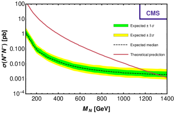
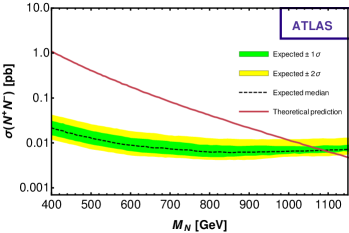
Figure 2: (a) CMS CMS:2019lwf and (b) ATLAS ATLAS:2020wop bounds on the Type-III fermions. The black dashed lines are the expected medians, whereas, the green and yellow bands present the $1\sigma$ and $2\sigma$ regions, respectively. For both the cases the red line denotes the theoretical prediction for the pair production of Type-III fermions.

Likewise, the Type-III seesaw model Foot:1988aq ; Ma:1998dn ; Ma:2002pf ; Hambye:2003rt ; Abada:2007ux ; Dorsner:2006fx ; Abada:2008ea ; He:2009tf ; Bandyopadhyay:2009xa ; Bandyopadhyay:2010wp consists of all the SM fields in addition to the three generations of colourless $SU(2)_{L}$ triplet (adjoint) fermions $(\Sigma_{L}\,(\bm{1,3},0))$ with hypercharge zero, mass $M_{\Sigma}$ and Yukawa coupling $\sqrt{2}\,Y_{\Sigma}$. The apposite pieces of Lagrangian are the following:

$$\begin{split}-\mathscr{L}_{III}\supset\frac{1}{2}{}&Tr[\hbox{\vbox{\hrule height=0.65pt\kern 1.72218pt\hbox{\kern-0.50003pt$\Sigma$\kern 0.0pt}}}_{L}M_{\Sigma}\,\Sigma_{L}^{\,c}]+\sqrt{2}\,Y_{\Sigma}\,\hbox{\vbox{\hrule height=0.65pt\kern 1.72218pt\hbox{\kern-0.50003pt$L$\kern 0.0pt}}}\,\Sigma_{L}^{c}\,\widetilde{H}+h.c.\,,\\ \text{with}{}&\quad\Sigma_{L}=\begin{pmatrix}\Sigma^{0}/\sqrt{2}&\Sigma^{+}\\ \Sigma^{-}&-\Sigma^{0}/\sqrt{2}\end{pmatrix}.\end{split}$$ (13)

After EWSB, the SM neutrinos mix with the neutral components of the fermionic triplet, while the charged ones mingle with the charged leptons. The mass matrices in flavour basis and the masses for all the leptons in energy basis are given by:

$$\mathcal{M}=\begin{pmatrix}0&\frac{v_{0}}{\sqrt{2}}Y_{\Sigma}\\ \frac{v_{0}}{\sqrt{2}}Y_{\Sigma}^{T}&M_{\Sigma}\end{pmatrix},\quad\mathcal{M}_{l^{\prime}}=\begin{pmatrix}m_{l^{\prime}}&v_{0}Y_{\Sigma}\\ 0&M_{\Sigma}\end{pmatrix},\quad$$

$$m_{\nu}\approx\frac{v_{0}^{2}}{2}\,Y_{\Sigma}\,M_{\Sigma}^{-1}\,Y_{\Sigma}^{T}\,,\quad m_{l}\approx m_{l^{\prime}},\quad M_{N^{0}}\approx M_{N^{\pm}}\approx M_{\Sigma}\,.$$ (14)

Here, $l^{\prime}$ denotes the SM charged leptons in flavour basis while $l$ and $N^{\pm}$ symbolise the same with the light and heavy masses in the mass-basis of Type-III scenario. Now, these heavy leptons will eventually decay to the lighter particles. While the heavy neutral particle $N^{0}$ will decay through $Z\nu$, $h\nu$ and $W^{\pm}l^{\mp}$ with the decay widths given by:

$$\Gamma^{Z\nu}_{N^{0}}\approx\Gamma^{h\nu}_{N^{0}}\approx\frac{1}{2}\Gamma^{Wl}_{N^{0}}\approx\frac{Y_{\Sigma}^{2}M_{\Sigma}}{32\pi}\leavevmode\nobreak\ ,$$ (15)

the heavy charged leptons $N^{\pm}$ decays to $Zl^{\pm}$, $hl^{\pm}$ and $W^{\pm}\nu$ with the following decay widths:

$$\Gamma^{Zl}_{N^{\pm}}\approx\Gamma^{hl}_{N^{\pm}}\approx\frac{1}{2}\Gamma^{W\nu}_{N^{\pm}}\approx\frac{Y_{\Sigma}^{2}M_{\Sigma}}{32\pi}\leavevmode\nobreak\ ,$$ (16)

where we have assumed that $M_{\Sigma}\gg m_{h}$ with $m_{h}$ being the mass of the SM Higgs boson around $125.5$ GeV. At this point, it is interesting to mention that though the masses of $N^{0}$ and $N^{\pm}$ are same at tree level, there can emerge a mass splitting of $\Delta M\approx 166$ MeV Cirelli:2005uq while considering the loop corrections and it can open up some decay channels of $N^{\pm}$ to $N^{0}$ with the decay width as follows:

$$\begin{split}\Gamma_{N^{\pm}}^{N^{0}\pi^{\pm}}=\frac{2G_{F}^{2}V_{ud}^{2}\Delta M^{3}f_{\pi}^{2}}{\pi}\sqrt{1-\frac{m_{\pi}^{2}}{\Delta M^{2}}}\quad\text{and}\\ \Gamma_{N^{\pm}}^{N^{0}e\,\nu_{e}}=\frac{25}{3}\Gamma_{N^{\pm}}^{N^{0}\mu\,\nu_{\mu}}=\frac{2G_{F}^{2}\Delta M^{5}}{15\pi^{3}}\leavevmode\nobreak\ ,\end{split}$$ (17)

where $f_{\pi}$ is the pion form factor, $m_{\pi}$ is the mass of pion, $G_{F}$ is the Fermi constant and $V_{ud}$ is the CKM matrix element. One should also notice here that none of the decay widths mentioned in Equation 17 depends on mass or Yukawa coupling of the $SU(2)$ triplet. However, for a TeV scale fermionic triplet with Yukawa greater than $10^{-7}$, one can safely neglect these modes due to very small branching fractions with $\lesssim 1\%$ Sen:2021fha .

Like the Type-I seesaw, in this case also, the demand of light neutrino mass being less than $0.1$ eV pushes the Yukawa coupling of TeV-scaled fermionic triplet to $\mathcal{O}(10^{-6})$, which is quite challenging to observe in the colliders. Therefore, we investigate for inverse Type-III scenario (iType-III), where three generations of two left handed fermionic triplets $(\Sigma_{a},\Sigma_{b})$ with only one of them interacting to SM leptons are introduced Ma:2009kh ; Eboli:2011ia ; Agostinho:2017biv ; Bandyopadhyay:2020djh . Here also there exists a large mixing between the flavour states $\Sigma_{a}\text{ and }\Sigma_{b}$. The corresponding relevant portions of the Lagrangian are given by:

$$-\mathscr{L}_{III}^{in}=\sqrt{2}Y\hbox{\vbox{\hrule height=0.65pt\kern 1.72218pt\hbox{\kern-0.50003pt$L$\kern 0.0pt}}}\Sigma_{a}^{c}\widetilde{H}+Tr[\;\hbox{\vbox{\hrule height=0.65pt\kern 1.72218pt\hbox{\kern-0.50003pt$\Sigma_{a}^{c}$\kern 0.0pt}}}M_{n}\Sigma_{b}+\frac{1}{2}\;\hbox{\vbox{\hrule height=0.65pt\kern 1.72218pt\hbox{\kern-0.50003pt$\Sigma_{b}^{c}$\kern 0.0pt}}}\,\mu_{n}\,\Sigma_{b}]+h.c.,$$ (18)

where the generation indices have been suppressed. While $Y$ denotes the Yukawa coupling of triplet $\Sigma_{a}$ with SM leptons, $M_{n}$ indicates the heavy mixing between $\Sigma_{a}\text{ and }\Sigma_{b}$ while small $\mu_{n}$ (complex symmetric matrix) signifies the mass of $\Sigma_{b}$. After the EWSB and mixing of the flavour states, there appear different mass eigenstates for the neutral as well as the charged leptons. Like the inverse Type-I scenario, here also one set of light neutrinos $(\nu)$ and two sets of heavy neutrinos ($N^{0},\widetilde{N}^{0}$), each set containing three generations, emerge. On the other hand, there also appear one set of light charged leptons $(l)$ and two sets of charged heavy leptons ($N^{\pm},\widetilde{N}^{\pm}$). The mass matrices in flavour basis and the masses of all these physical states are as follows:

$$\begin{split}\mathcal{M}=\begin{pmatrix}0&\frac{v_{0}}{\sqrt{2}}Y&0\\ \frac{v_{0}}{\sqrt{2}}Y^{T}&0&M_{n}\\ 0&M_{n}^{T}&\mu_{n}\end{pmatrix},{}&\quad\mathcal{M}_{l^{\prime}}=\begin{pmatrix}m_{l^{\prime}}&v_{0}Y&0\\ 0&0&M_{n}\\ 0&M_{n}^{T}&\mu_{n}\end{pmatrix},\\ m_{\nu}\approx\frac{v_{0}^{2}}{2}\,Y(M_{n}^{-1})^{T}\mu_{n}\,M_{n}^{-1}{}&Y^{T},\quad m_{l}\approx m_{l^{\prime}}\quad\text{ and }\\ M_{N^{0}/\widetilde{N}^{0}}^{2}\approx M_{N^{\pm}/\widetilde{N}^{\pm}}^{2}{}&\approx M_{n}\,M_{n}^{T}\,.\end{split}$$ (19)

where $l^{\prime}$ denotes the flavour states of SM charged leptons. Similar to the Type-I case, one can easily satisfy the neutrino bounds with suitable choice of $\mu_{n}$ while considering $Y\sim\mathcal{O}(0.1)$ and $M_{n}\sim\mathcal{O}(1$ TeV).

The heavy leptons will finally decay to the light(SM) leptons associated with the Higgs boson or the weak gauge bosons. The partial decay widths of each generation of $N^{0}$ and $\widetilde{N}^{0}$ in different channels are given by:

$$\Gamma^{Z\nu}_{N^{0}/\widetilde{N}^{0}}\approx\Gamma^{h\nu}_{N^{0}/\widetilde{N}^{0}}\approx\frac{1}{2}\Gamma^{Wl}_{N^{0}/\widetilde{N}^{0}}\approx\frac{Y^{2}M_{n}}{64\pi}\leavevmode\nobreak\ .$$ (20)

As already mentioned in subsection 2.1, the partial decay widths of heavy neutrinos in this case will be half of the same in usual Type-III scenario. Another interesting feature can be observed in the behaviour of the neutral and the charged components of iType-III fermion; unlike the neutral components $N^{0}/\widetilde{N}^{0}$, which couples to $Z,\,h$ and $W^{\pm}$ (Equation 20), one of the charged components, $N^{\pm}$ couples to $Z\ell$ and $h\ell$ only, while the other one, $\widetilde{N}^{\pm}$ interacts with $W^{\pm}\nu$ (see Appendix A). This indicates the decay of $N^{\pm}$ through $hl$ and $Zl$ modes with $50\%$ branching in each but $\widetilde{N}^{\pm}$ decays to $W\nu$ entirely. The partial decay widths for the charged components are given by:

$$\Gamma^{Zl}_{N^{\pm}}\approx\Gamma^{hl}_{N^{\pm}}\approx\frac{1}{2}\Gamma^{W\nu}_{\widetilde{N}^{\pm}}\approx\frac{Y^{2}M_{n}}{32\pi}\leavevmode\nobreak\ .$$ (21)

The ATLAS and CMS collaborations have already    searched for the existence of heavy charged (neutral) leptons at LHC. Non-observation of any such state force them to put experimental upper bounds on the pair production cross section as a function of heavy lepton mass. However, the theoretical cross section, predicted there, involves one generation of heavy lepton only, whereas, in our case there are six copies of heavy charged (neutral) leptons. Therefore, we scale the theoretical estimate lines of Refs. CMS:2019lwf ; ATLAS:2020wop by six and reproduce the plots in Figure 2, where the black dashed lines indicate expected median, the green and yellow regions signify the $1\sigma$ and $2\sigma$ expectations respectively while the red curve symbolizes the theoretical estimation of the pair production cross section with six copies of heavy charged leptons. Considering both the results from ATLAS and CMS, we can restrict the mass of fermionic triplet in inverse Type-III case (three generations) to be higher than 1100 GeV with $2\sigma$ values of expectation.

3 Angular distributions

It is known that the angular distribution in the centre of mass (CM) frame carries information about the matrix elements, and the information of spin of initial and finalstate particles, propagator as well as vertices are also encoded. It has been shown that spins of different BSM particles can be discerned via such angular distributions Datta:2005zs ; Battaglia:2005ma ; Christensen:2013aua . However, such distribution at the hadronic collider like LHC has certain disadvantage of not knowing the centre of mass frame due to unknown initial state boost along the beam axis, and reconstruction of the CM frame is only possible if the finalstate is fully visible. An interesting feature of such distribution with a massless gauge boson in the initial or finalstate can give rise to zeros in amplitude (RAZ) of the matrix element Brodsky:1982sh . Thus the angular distribution vanishes at certain angle depending on the charges and four momenta of the associate particles, and particles with fractional electromagnetic charges, like leptoquakrs, can be distinguished via such angular distributions Bandyopadhyay:2020jez ; Bandyopadhyay:2020klr ; Bandyopadhyay:2020wfv . In this article we explore such possibilities in various leptonic colliders as they are automatically in the centre of mass frame for the symmetric collisions.

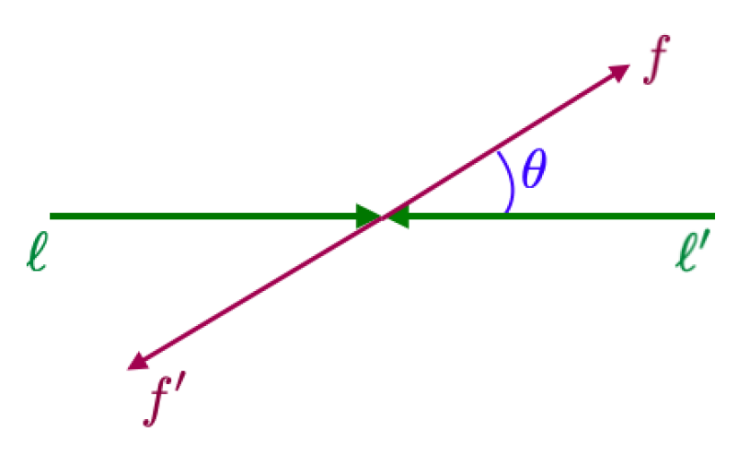
Figure 3: Schematic diagram of the initial and finalstate particles in the leptonic collider. The polar angle of one of the finalstate particles with the beam axis, which can be measured in the centre of mass frame of the leptonic collider, is denoted by $\theta$.

A typical collision is shown in Figure 3, where charged leptons $\ell\ell^{\prime}$ are collided to produce leptonic finalstate $ff^{\prime}$ and $\theta$ is the angle made by finalstate particle $f$ with the beam axis ($z$-axis). The differential distribution with respect to $\cos{\theta}$ is going to be instrumental in discerning various seesaw scenarios as we discuss them in the following sections.

4 Set up for collider simulation

At first, the models are implement at SARAH-4.14.2 Staub:2013tta and model files for CalcHEP Belyaev:2012qa are prepared. The branching fractions and production cross-sections for different BSM particles are estimated through CalcHEP. Then we generate events for different relevant modes via CalcHEP and use the generated “.lhe” files as an input to PYTHIA8 Sjostrand:2007gs ; Sjostrand:2014zea where the events are simulated with FastJET-3.0.3 Cacciari:2011ma . The following criteria are being maintained during the simulation:

1. Though we are interested in the angular distribution of various channels for the whole region, to avoid beam line events we restrict the calorimeter coverage for $|\eta|<4.5$.

2. Regarding jet formation, we use:

   • The ANTI-KT algorithm with the jet radius $R=0.5$.

   • The minimum transverse momentum for jets $p_{T,\text{min}}^{\text{jet}}=20\,\text{GeV}$.

3. The stable leptons are detected with following cuts:

   • The minimum transverse momentum of the leptons $p_{T,min}=10\,\text{GeV}$ with $|\eta_{\text{max}}|=4.5$.

   • The leptons are isolated from the jet with $\Delta R_{\ell j}\geq 0.4$, where $\Delta R_{\ell j}=\sqrt{\Delta\eta_{\ell j}^{2}+\Delta\phi_{\ell j}^{2}}$ .

   • For a selection of clean lepton, we put an additional cut i.e., the total transverse momentum of the hadrons within the cone $\Delta R=0.3$ will be $\leq 0.15\;p_{T}^{\ell}$. Here $p_{T}^{\ell}$ is the transverse momentum for the leptons within that specified cone.

4. We have already denoted $l$ as all the three generations of SM charged leptons in mass basis. However, most of our upcoming discussions are based on electron and muon only. Therefore, we symbolize these two leptons as $\ell$.

5 At $\ell^{-}\ell^{-}$ collider

Type-I seesaw is very hard to detect at $\ell^{-}\ell^{-}$ collider. However, there is production of SM finalstate i.e., $\ell^{-}\ell^{-}\to W^{-}W^{-}$, where the BSM particles in principle can play a major role. This process is completely absent in SM, due to non-existence of any Majorana fermion or doubly charged particle. Therefore, a departure from SM prediction along with the difference in angular distributions can hint a new physics signal. This is illustrated in Figure 4, where $\ell^{-}\ell^{-}\to W^{-}W^{-}$ for iType-I and iType-III seesaw are mediated by $N^{0}/\widetilde{N}^{0}\,$ and for Type-II seesaw it is mediated by $\Delta^{--}$ in $s$-channel. In case of the Type-I seesaw, $\ell^{-}\ell^{-}\to W^{-}W^{-}$ cross-section is proportional to $(Y_{\nu}^{2}/M_{R})^{2}$ and as mentioned earlier, $Y_{\nu}$ has to be very small or $M_{R}$ has to be very large in order to keep neutrino mass $\mathcal{O}(10^{-1}\text{ eV})$, which result in a vanishingly small cross-section. In case of the inverse seesaw, the destructive interference takes place between the t-channel diagrams mediated by $N^{0}$ and $\widetilde{N}^{0}$, which in turn keeps the cross-section very low. Similar situation arises for the Type-III scenario also for the same channel. In case of the Type-II scenario, the additional contribution for this mode comes from the doubly charged scalar particle in s-channel. However, the $\ell^{-}\ell^{-}\Delta^{++}$ vertex is proportional to $Y_{\Delta}$, whereas the $W^{-}W^{-}\Delta^{++}$ vertex is commensurate with $v_{\Delta}$ eventuating in cross-section proportional to $v_{\Delta}^{2}Y_{\Delta}^{2}\sim\frac{1}{2}m_{\nu}^{2}$ (see Equation 8). Therefore, in the case of Type-II, such cross-section is vanishingly small.

Figure 4: Feynman diagrams for $\ell^{-}\ell^{-}\to W^{-}W^{-}$ in iType-I and iType-III seesaw (first and second panel with $N^{0}/\widetilde{N}^{0}\,$ mediator) and in Type-II seesaw (third panel with $\Delta^{--}$ mediator).

It is interesting to see that, $\ell^{-}\ell^{-}$ can still be instrumental in distinguishing at least Type-II and iType-III seesaw mechanisms via the finalstates involving leptons of different flavours (see Figure 5) or involving at least one BSM heavy leptons (see Figure 10) as detailed in the following subsections.

Multi-TeV Muon collider is proposed Ankenbrandt:1999cta ; Delahaye:2019omf ; Bartosik:2019dzq ; AlAli:2021let ; Bartosik:2020xwr with the reach around 10 ab^-1 for 10 TeV centre of mass energy. The advantage of the muon collider over the electron is that the former has much less synchrotron radiation. Generically leptonic colliders are free from any initial state QCD radiation. Due to the proposed reach in energy and luminosity, many beyond Standard Model scenarios are looked at the forthcoming muon collider Costantini:2020stv ; Buttazzo:2018qqp ; Huang:2021biu ; Huang:2021nkl ; Asadi:2021gah ; Capdevilla:2020qel ; Capdevilla:2021rwo ; Long:2020wfp ; Han:2020pif ; Han:2020uak ; Han:2021udl ; Bandyopadhyay:2021pld . In this case also the collisions happen in the CM frame, making it easier to construct the angular distributions for the finalstate in the CM frame. Hence, we use muon beams as the initial states for our simulation. Regarding our analysis at this collider, we choose three different centre of mass energies which are 1.5 TeV (BP1), 2.0 TeV (BP2) and 3.0 TeV (BP3), respectively as tabulated in Table 1 (Type-II) and Table 3 (iType-III), with an integrated luminosity of 1000 fb^-1. However, the masses of the BSM particles are chosen differently in different scenarios in order to obtain significant number of events.

5.1 Type-II seesaw

Figure 5: Feynman diagram for $\ell^{-}\ell^{-}\to\ell^{\prime-}\ell^{\prime-}$.

In the Type-II seesaw at $\ell^{-}\ell^{-}$ collider, the mode $\ell^{-}\ell^{-}\to\ell^{\prime-}\ell^{\prime-}$ that occurs through $\Delta^{--}$ mediated s-channel diagram, as depicted in Figure 5. Unlike the $W^{-}W^{-}$ channel, the advantage of this mode is that both the vertices in this case are proportional to $Y_{\Delta}$ only. However, since this mode is mediated through s-channel only, the cross-section would reduce significantly if we move away from the resonance production. The cross-section and the angular distribution with respect to $x=\cos{\theta}$ for this mode in CM frame are given by:

$$\sigma(\ell^{-}\ell^{-}\to\ell^{\prime-}\ell^{\prime-}) =\int_{0}^{1}\frac{d\sigma}{dx}(\ell^{-}\ell^{-}\to\ell^{\prime-}\ell^{\prime-})dx$$

$$=\frac{s\,Y_{\Delta}^{4}}{128\pi[(s-M_{\Delta}^{2})^{2}+M_{\Delta}^{2}\Gamma_{\Delta}^{2}]},$$ (22)

where, $\sqrt{s}$ is the centre of mass energy, $\Gamma_{\Delta}\big{(}\approx\frac{3M_{\Delta}Y_{\Delta}^{2}}{32\pi}\big{)}$ is the total decay width of $\Delta^{--}$ (branching of di-bosons are negligible, since, $v_{\Delta}$ is very small for our benchmark scenarios) and $\theta$ is the angle between the beam axis and anyone of the finalstate electrons with $x\equiv\cos\theta$. It is interesting to mention here that the angle $\theta$ in this case will vary from 0 to $\pi/2$ only, since the two particles in final state are indistinguishable.

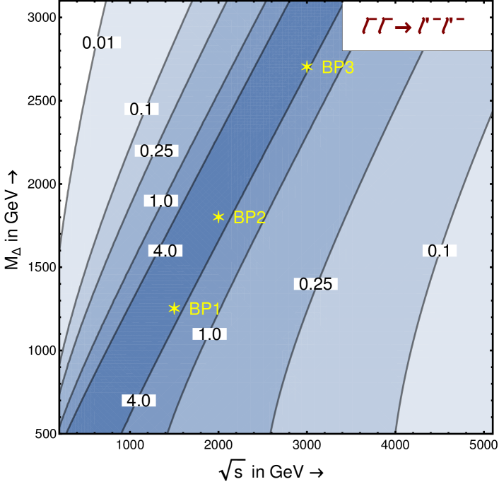
Figure 6: Variation of total cross-section (in fb) for the process $\ell^{-}\ell^{-}\to\ell^{\prime-}\ell^{\prime-}$, with respect to centre of mass energy and mass of the triplet in Type-II seesaw scenario ($Y_{\Delta}=0.2$, $\mu_{\Delta}=10$ eV). The three benchmark points are represented by the yellow stars.

	$\sigma(\mu^{-}\mu^{-}\to e^{-}e^{-})$
Benchmark	$M_{\Delta}$	$E_{CM}$	Cross-section
Points	in GeV	in TeV	(in fb)
BP1	1250	1.5	7.4
BP2	1800	2.0	10.7
BP3	2700	3.0	4.8

Table 1: Masses corresponding to different benchmark points, energy of collision in CM frame and the hard scattering cross-sections (in fb) for $e^{-}\,e^{-}$ final states in Type-II seesaw model and $\mu^{-}\mu^{-}$ collider. ($Y_{\Delta}=0.2$, $\mu_{\Delta}=10$ eV)

         

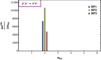
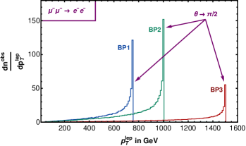
Figure 7: (a) multiplicity ($n_{\rm lep}$) distributions for the charged leptons and (b) the transverse momentum ($p_{T}^{\rm lep}$) distribution for the benchmark points at the centre of mass energies of 1.5, 2.0, 3.0  TeV, respectively with the integrated luminosity of 1000 fb^-1. $p_{T}^{\rm lep}$ distribution is same for the two leptons for the benchmark points as they are identical, which can be depicted from Figure 5.

In Figure 6, we describe the variation of total cross-section for the process $\ell^{-}\ell^{-}\to\ell^{\prime-}\ell^{\prime-}$ as given in Figure 6, with respect to centre of mass energy and mass of the triplet in the Type-II seesaw scenario. The darker to faint colours represent from large to less cross-sections. It is interesting to notice that, as $M_{\Delta}$ approaches $\sqrt{s}$, the cross-section enhances largely due to the resonance production of the doubly charged scalar and the three benchmark points are chosen near the resonance production allowed by the collider bounds as tabulated in Table 1.

However, this mode is completely non-existent in Type-I, ISS cases, and also in Type-III, iType-III scenarios if $Y$ and $M_{n}$ are assumed diagonal. Although there is a possibility for its occurrence in iType-III picture under non-diagonal $Y$ or $M_{n}$, the cross-section is severely low due to the fact that $\hbox{\vbox{\hrule height=0.65pt\kern 1.72218pt\hbox{\kern-0.50003pt$\ell$\kern 0.0pt}}}\ell^{\prime}Z$ coupling is quadratic in the ratio of Dirac mass term to the mass of heavy neutrinos after EWSB (i.e. $M_{D}^{\dagger}[M_{n}^{\dagger}M_{n}]^{-1}M_{D}$, where $M_{D}$, the Dirac mass term for neutrinos, is given by $\frac{v_{0}}{\sqrt{2}}Y$, in comparison with the Type-II coupling $\ell^{-}\ell^{-}\Delta^{++}$, proportional to $Y_{\Delta}$. Therefore, observation of this mode will advocate for the presence of Type-II seesaw.

Regarding our simulation, we choose muon collider as explained before with the triplet mass $M_{\Delta}$ to be 1.25 TeV, 1.8 TeV and 2.7 TeV, respectively for the three benchmark points. Taking the Yukawa $Y_{\Delta}=0.2$ (and $\mu_{\Delta}=10$ eV) the cross-sections of the process $\mu^{-}\mu^{-}\to e^{-}e^{-}$ in the CM frame for the benchmark points are 7.4 fb, 10.7 fb and 4.8 fb, respectively, as tabulated in Table 1.

Equipped with the setup for the collider simulation as described in section 4, we describe the different kinematical distributions relevant to our analysis in the following paragraphs. In Figure 7(a), we illustrate charged lepton multiplicity and their transverse momentum distribution are shown in Figure 7(b) for all the three benchmark points. Since there is no SM background as well as model background, we observe all the events with lepton multiplicity two only. On the other hand the transverse momentum distribution of the charged leptons can be expressed as:

$$\Big{|}\frac{dn^{obs}}{dp_{T}^{lep}}\Big{|}=\Big{|}\frac{\tan\theta}{p^{lep}}\cdot\frac{dn^{obs}}{d\cos\theta}\Big{|}\propto\tan\theta,$$ (23)

where $p^{lep}(\equiv E_{CM}/2)$ is the total three momentum of a finalstate lepton and $(dn^{\rm obs}/d\cos\theta)$ is independent of $\theta$ which is obvious from subsection 5.1. At small values of $\theta$, the transverse momentum of a finalstate lepton becomes small and the transverse momentum distribution also remains small since it is proportional to $\tan\theta$, shown above. However, at $\theta\to\pi/2$, the transverse momentum of a finalstate lepton reaches its maximum value, i.e. $E_{CM}/2$, and the transverse momentum distribution blows up due to divergence in $\tan\theta$, as can be noticed from Figure 7(b).

We simulate this channel in PYTHIA8 Sjostrand:2007gs for the three mentioned benchmark points with an integrated luminosity of 1000 fb^-1 and search for same sign di-electron signature. As mentioned earlier, there is no SM background as well as model background for this process. The signal numbers for this finalstate with the three benchmark points are presented in Table 2, which are very heartening.

Final state	BP1	BP2	BP3
$2e^{-}$	7368.5	10727.8	4767.8

Table 2: Number of events for $2e^{-}$ final state for the benchmark points mentioned in Table 1 with the integrated luminosity of 1000 fb^-1.

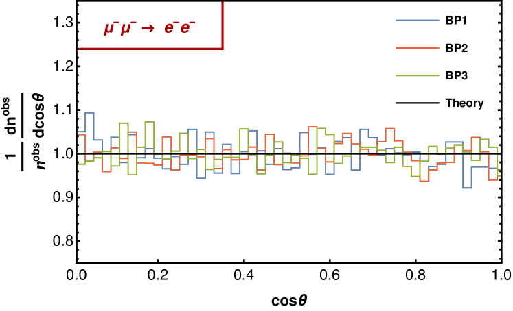
Figure 8: Angular distribution of the finalstate $e^{-}$ for the benchmark points at the centre of mass energies of 1.5, 2.0, 3.0  TeV, respectively. The blue, red, green histograms depict the simulated results for BP1, BP2, BP3, respectively and the black line signifies the theoretical estimation.

The normalised angular distribution for this channel is presented in Figure 8, where the blue, green and red lines indicate the simulated results for three benchmark points, respectively and the black straight line signifies the theoretical estimation. It can be noticed that the simulated results matches quite well with the theoretical prediction and this flat angular distribution of finalstate electrons relative to the angle with beam axis is the distinctive signature for the presence of doubly charged scalar $\Delta^{--}$ in the s-channel propagator which in turn would imply the existence of Type-II seesaw.

At this point it is important to mention that one can also use Radiation Amplitude Zero (RAZ) Brodsky:1982sh through the $\ell^{-}\ell^{-}\to\gamma\,\Delta^{--}$ channel to probe the existence of Type-II scenario. With our benchmark points the cross-sections for this process are also large. The angular distribution of the photon will look like a tub with the RAZ occurring at $\cos\theta=0$ implying $\theta=90^{\circ}$ with respect to the beam axis as shwon in Figure 9.

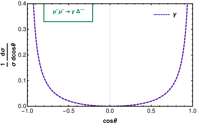
Figure 9: Normalised angular distribution of the photon in the process $\ell^{-}\ell^{-}\to\gamma\,\Delta^{--}$ with $Y_{\Delta}=0.2$, $M_{\Delta}=1250$ GeV and the centre of mass energy of 1.5 TeV.

5.2 Type-III seesaw (inverse)

Figure 10: Feynman diagrams for $\ell^{-}\ell^{-}\to\ell^{-}N^{-}$.

In this section, we separate out the signature of inverse Type-III seesaw at $\ell^{-}\ell^{-}$ collider. The peculiarity of iType-III seesaw model is that it contains heavy charged leptons ($N^{\pm}$) along with heavy neutrinos ($N^{0}$) and by probing these heavy charged leptons one can discriminate the iType-III scenario. For this purpose, footprints of the scattering process $\ell^{-}\ell^{-}\to\ell^{-}N^{-}$, that occurs through Z boson mediated t and u channel diagrams, as displayed in Figure 10, should be traced. In principle, it could occur through $h$-mediation also; but since $\ell^{+}\ell^{-}h$ coupling very small for the light leptons, one can safely ignore it. At this point it should be noted that inverse Type-III seesaw contains six copies of heavy charged leptons; however, as mentioned in subsection 2.3, three of them ($N^{\pm}$) couples to $Z$ and $h$, and the rest three ($\widetilde{N}^{\pm}$) couple to $W$-boson only. As the mentioned process is predominantly $Z$-mediated, $\widetilde{N}^{\pm}$ will never be produced through $\ell^{-}\ell^{-}$ collision. Moreover, we have considered diagonal coupling only. Therefore, for a particular initial state, only one type of $N^{-}$ will get produced. The angular distribution and total cross-section this process are given by:

$$\frac{d\sigma}{dx}({\ell^{-}\ell^{-}\to\ell^{-}N^{-}})=\frac{m_{Z}^{4}Y^{2}\lambda^{2}}{4\pi sv_{0}^{2}M_{n}^{2}(\zeta^{2}-\lambda^{2}x^{2})^{2}}\Big{[}2\zeta^{2}(1-2S_{w}^{2})^{2}$$

$$\hskip 28.45274pt+S_{w}^{4}\big{\{}(1-x^{2})(2\zeta^{2}-\lambda\zeta^{2}-x^{2}\lambda^{3})+2x^{2}(\zeta+\lambda)^{2}\big{\}}\Big{]},$$

$$\sigma({\ell^{-}\ell^{-}\to\ell^{-}N^{-}})=\frac{m_{Z}^{4}Y^{2}\lambda}{4\pi sv_{0}^{2}M_{n}^{2}}\Big{[}\frac{\lambda(1-2S_{w}^{2})^{2}}{\zeta^{2}-\lambda^{2}}+2S_{w}^{4}\Big{(}1+\frac{1}{\zeta-\lambda}\Big{)}$$

$$\hskip 28.45274pt+\Big{\{}\frac{1}{\zeta}(1-2S_{w}^{2})^{2}-2S_{w}^{4}\frac{(1+\zeta)}{\lambda}\Big{\}}\tanh^{-1}\Big{(}\frac{\lambda}{\zeta}\Big{)}\Big{]},$$ (24)

where, $S_{w}=\sin\theta_{w}$ , $\lambda=1-\frac{M_{n}^{2}}{s}$ , $\zeta=1+\frac{2}{s}(m_{Z}^{2}-M_{n}^{2})$ with $m_{Z}$ being the mass of Z bosons, $\theta_{w}$ the Weinberg angle and $x$ is the cosine of angle between final state electron and beam axis.

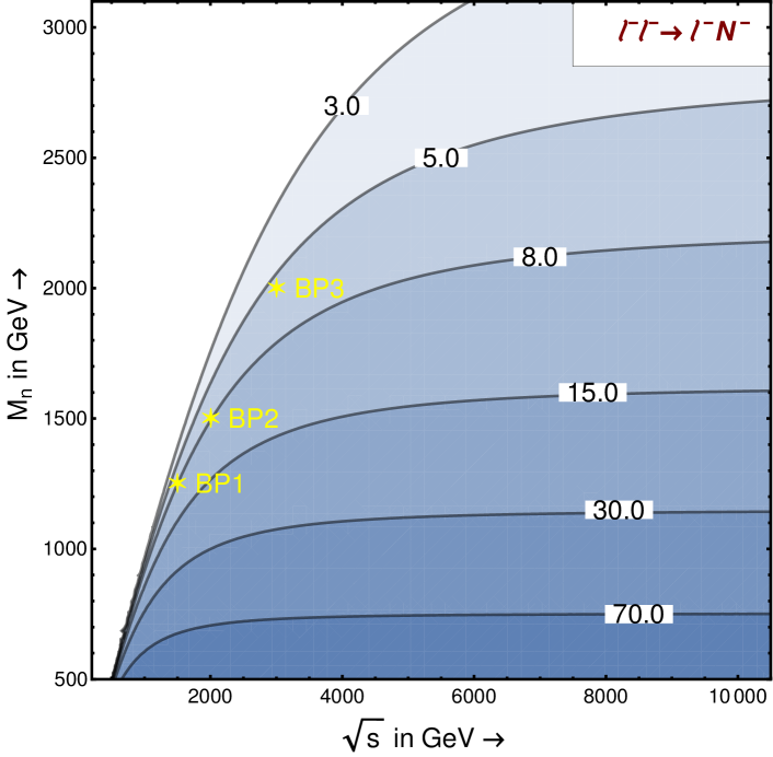
Figure 11: Variation of total cross-section (in fb) for the process $\ell^{-}\ell^{-}\to\ell^{-}N^{-}$, with respect to the centre of mass energy and mass of the triplet in the Type-III seesaw scenario ($Y=0.2$, $\mu_{n}=10$ eV). The three benchmark points are represented by the yellow stars.

	$\sigma(\mu^{-}\mu^{-}\to\mu^{-}N^{-})$
Benchmark	$M_{n}$	$E_{\rm CM}$	Cross-section
Points	in GeV	in TeV	(in fb)
BP1	1250	1.5	8.8
BP2	1500	2.0	8.6
BP3	2000	3.0	6.1

Table 3: Masses corresponding to different benchmark points, energy of collision in CM frame and the hard scattering cross-sections (in fb) for $\mu^{-}N^{-}$ final state in Type-III seesaw model and $\mu^{-}\mu^{-}$ collider. ($Y=0.2$, $\mu=10$ eV)

Figure 11 shows the variation of total cross-section for the process $\ell^{-}\ell^{-}\to\ell^{-}N^{-}$, with respect to the centre of mass energy and mass of the triplet fermion in the iType-III seesaw scenario with $Y=0.2$, $\mu_{n}=10$ eV. The darker to fainter blue regions represent larger to lesser cross-sections. The cross-section decreases as the mass of the triplet fermion increases, keeping the centre of mass energy constant. On the other hand, the cross-section increases with the increase of centre of mass energy for a fixed mass. Because of unavailability of enough phase space, the cross-section is zero, if $s\leq M_{n}^{2}$.

It should be noted that one can also look for the process $\ell^{-}\ell^{-}\to N^{-}N^{-}$ for detection of iType-III seesaw, but the cross-section is quite small due to the fact that on both legs we need $\ell^{\pm}-N^{\pm}$ mixings proportional to the Yukawa coupling $Y$ and also due to the reduction of the the available phase space as compared to $\ell^{-}N^{-}$ mode. Now, as mentioned in subsection 2.3 and Appendix A, this heavy charged leptons ($N^{-}$) will eventually decay to $Z\,\ell^{-}$ or $h\,\ell^{-}$. Therefore, observation of any peak in the invariant mass distribution for $jj\ell/bb\ell$ around heavy lepton mass via the reconstruction of $Z/h$ peaks will confirm the existence of heavy charged leptons, hence the Type-III seesaw.

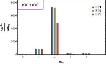
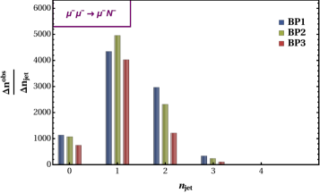
Figure 12: Multiplicity distributions, (a) for the charged leptons ($n_{\rm lep}$) and (b) for the jets ($n_{\rm jet}$) for the benchmark points at the centre of mass energies of 1.5, 2.0, 3.0  TeV, respectively with the integrated luminosity of 1000 fb^-1.

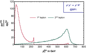
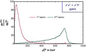
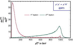
Figure 13: Transverse momentum distribution of the $1^{\rm st}$ and $2^{\rm nd}$ charged leptons ($p_{T}^{\rm lep}$), (a) BP1, (b) BP2 and (c) BP3 at the centre of mass energies of 1.5, 2.0, 3.0  TeV, respectively with the integrated luminosity of 1000 fb^-1.

For our collider analysis, we have considered three different values of $M_{n}$, which are 1.25 TeV, 1.5 TeV and 2.0 TeV, respectively, for three benchmark points as shown with the yellow star in Figure 11 with the Yukawa coupling $Y=0.2$ and $\mu_{n}=10$ eV. As listed in Table 3, the cross-sections for the process $\mu^{-}\mu^{-}\to\mu^{-}N^{-}$ in the CM frame for the three benchmark points are 8.8 fb, 8.6 fb and 6.1 fb, respectively.

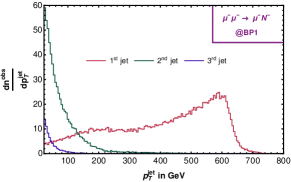
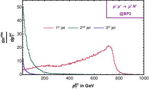
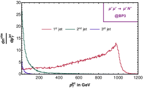
Figure 14: Transverse momentum distribution of the $1^{\rm st}$, $2^{\rm nd}$ and $3^{\rm rd}$ $p_{T}$ ordered jets ($p_{T}^{\rm jet}$), (a) BP1, (b) BP2 and (c) BP3 at the centre of mass energies of 1.5, 2.0, 3.0  TeV, respectively with the integrated luminosity of 1000 fb^-1.

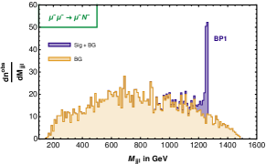
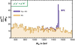
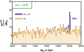
Figure 15: Di-jet-mono-lepton invariant mass distribution ($M_{jj\ell}$) for (a) BP1, (b) BP2 and (c) BP3 at the centre of mass energies of 1.5, 2.0, 3.0  TeV, respectively with the integrated luminosity of 1000 fb^-1. The total (signal $+$ SM background) signature is depicted in blue and the SM background is in yellow.

Final states	BP1		BP2		BP3
	Sig	BG	Sig	BG	Sig	BG
$2\ell+2j$	2459.0	$1.49\times 10^{5}$	1779.0	$1.30\times 10^{5}$	721.0	$1.01\times 10^{5}$
$+|M_{jj\ell}-M_{n}|\leq 10\,$GeV	806.1	178.0	565.2	238.2	199.2	127.9
$\rm{S}_{\text{sig}}(\mathcal{L}_{\rm int}=1000\,\rm fb^{-1})$	25.7		19.9		11.0
$\int\mathcal{L}_{5\sigma}\,[\rm{fb}^{-1}]$	37.9		63.1		206.6

Table 4: Number of events for signal and background corresponding to $2\ell+2j$ final state for the benchmark points mentioned in Table 3 with the integrated luminosity of 1000 fb^-1.

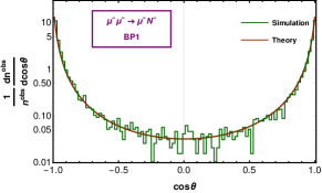
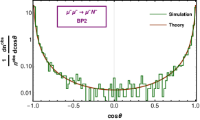
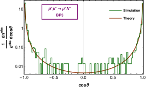
Figure 16: Angular distribution of the reconstructed heavy charged fermion from $M_{jj\ell}$ invariant mass for (a) BP1, (b) BP2 and (c) BP3 at the centre of mass energies of 1.5, 2.0, 3.0  TeV, respectively. The green histograms depict the simulated result and the brown lines signify the theoretical estimation.

Regarding kinematic distributions of this process, we exhibit the lepton multiplicity and jet multiplicity in the left and right panel of Figure 12, where the blue, green and red columns indicate the three benchmark points, respectively. The other charged lepton either can come from the $N^{-}$ decays to $Z/h,\ell^{-}$ or $W^{-},\nu$ and the further decays of $Z,W^{-}$ bosons. This results in peaking of charged lepton distribution at two as can be seen from Figure 12(a). However, due to thee choice of heavy mass for the $N^{-}$, the jets coming from the Higgs or weak gauge boson decays are often collimated resulting a peak around one as depicted in Figure 12(b).

In Figure 13, we illustrate the transverse momentum distribution for this process with three panels describing three benchmark points. There are mainly two light leptons involved in this channel: 1) the one that gets produced associated with $N^{-}$ (red), 2) the one which is generated from the decay of $N^{-}$ (green). The first kind of light leptons will have low energies since lions share of the total energy will be carried by the massive particle $N^{-}$. The energy carried by this kind of leptons is given by:

$$E_{\ell_{1}}=\frac{s-M_{n}^{2}}{2\sqrt{s}},$$ (25)

the values of which are 230 GeV, 440 GeV and 830 GeV respectively for the three benchmark points. Due to the presence of $\tan\theta$ in the expression of lepton $p_{T}$ distribution (see Equation 23), $\theta$ being the angle of the light lepton with beam axis, we observe a slight bump in distribution near $p_{T}^{lep}=E_{\ell_{1}}$. The red line beyond this value of $p_{T}^{lep}$ arises because of misidentification of the second kind leptons as the first kind, which is obvious from the fact that they show small peaks at the same $p_{T}^{lep}$, where the green curves reach their maxima. Because of the typical angular distribution of this process, large number of events for this process lie around $\cos\theta\sim\pm 1$, which implies low $p_{T}$ for first kind of leptons. Therefore, we see a pile up of events in the low $p_{T}$ region of the red curves. On the other hand, the leptons coming from the decay of $N^{-}$ (green) possess relatively higher transverse momentum and the distribution peaks around $M_{n}/2$.

Similarly, in Figure 14, we display the jet $p_{T}$ distribution of this process with three benchmark points in three panels. As explained earlier, the two jets come from the Higgs and $Z$-boson decays, which essentially come from the decay of $N^{-}$. Since $N^{-}$ is very heavy, the jets will be very boosted and in most of the cases the two jets coming from $Z/h$ will be identified as a fatjet Sen:2021fha ; Chakraborty:2018khw ; Bhardwaj:2018lma ; CS:TypeI ; Bandyopadhyay:2010ms ; Ashanujjaman:2021zrh ; Ashanujjaman:2022cso . Therefore, we observe peaks around $M_{n}/2$ for the red curve in all the panel. The distributions of second and third jets, which appear with isolation of both the jets, fall off very rapidly with larger $p_{T}^{jet}$.

In the $\mu^{-}\mu^{-}$ collider, thus we should look for same sign di-lepton plus di-jet signature in order to detect Type-III scenario. In this case the $N^{-}\to W^{-}\nu$ fails to contribute any more (see subsection 2.3 and Appendix A) and the main contributions come from $N^{-}\to h/Z\ell^{-}$. The dominant SM background in this case will be $\mu^{-}\mu^{-}\to\mu^{-}\mu^{-}Z(\to jj)$. Nonetheless, constructing the invariant mass of $jj\ell$ system, one can significantly reduce the SM background. In Figure 15, we plot the invariant mass of $jj\ell$ for all the three benchmark points, where the yellow regions represent SM background and the blue portions indicate signal plus background. It can be easily seen that the blue curves exhibit sharp peak around $M_{n}$ while the yellow curves show continuum.

The signal-background analysis for this finalstate with an integrated luminosity of 1000 fb^-1 is presented in Table 4. As can be noticed, for same sign di-lepton plus di-jet signature, a huge of number of SM background arises from the SM background; however, with the invariant mass cut of $|M_{jj\ell}-M_{n}|\leq 10$ GeV, it drops off very quickly. Therefore, signal significance of more than 10$\sigma$ can be achieved in all the three benchmark points with 1000 fb^-1 of integrated luminosity. In other words, very early data of a few 100 fb^-1 can provide $5\sigma$ significance for all the three benchmark points in this case.

Now, we plot the angular distribution of the reconstructed particle from $M_{jj\ell}$ mass (or equivalently the muon produced in association with the heavy charged lepton) for all the three benchmark points and present them in Figure 16. In each of the plots, the green line indicates the simulated result while the brown curve signifies the theoretical estimation (via parton level and tagging $N^{-}$) of the distribution, and both the lines are in agreement with each other. In contrast to the angular distribution of finalstate muon in Type-II scenario (which looks flat in Figure 8), here the distribution looks like a tub with more number of events in the peripheral region (i.e. $|\cos\theta|\sim 1$) and less number of events in central region (i.e. $|\cos\theta|\sim 0$).

6 At $\ell^{+}\ell^{-}$ collider

The $\ell^{+}\ell^{-}$ colliders have great achievements in the history of Particle Physics. The LEP was very successful in providing the correctness of the SM through electroweak precision measurements. There are various proposed $e^{+}e^{-}$ colliders, like ILC Asner:2013psa ; Bambade:2019fyw , CLIC Aicheler:2018arh ; Kemppinen:2021urj , FCC-ee Blondel:2021ema ; Blondel:2019yqr ; Zimmermann:2015mea ; Boscolo:2021hsq , which are going to be built in near future . There is a very big problem with $e^{+}e^{-}$ colliders: due to the negligible mass of electron, it loses large portion of its energy while moving inside a circular collider and hence, very high centre of mass energy cannot be reached. To overcome this issue linear accelerators like ILC and CLIC have been proposed. Furthermore, the idea of $\mu^{+}\mu^{-}$ collider has also been put forward Ankenbrandt:1999cta ; Delahaye:2019omf ; Bartosik:2019dzq ; AlAli:2021let ; Bartosik:2020xwr . Due to non-negligible mass of muon, the synchrotron radiation would not be very high in this case and almost 30 TeV of centre of mass energy could be reached in this kind of collider. Additionally, large number of muons are getting produced in JPARC Abe:2019thb which would help to obtain an integrated luminosity of 10 ab^-1 at the muon collider.

For our analysis, we have used a muon collider with an integrated luminosity of 1000 fb^-1 and centre of mass energies of 2.5 TeV, 5.0 TeV and 8.0 TeV, respectively for the three benchmark points. In this case also the masses of different BSM particles are chosen differently. The Yukawa couplings of BSM particles are also assumed to be diagonal with value 0.2.

6.1 Type-I seesaw (inverse)

Figure 17: Feynman diagrams for dominant contribution to $\ell^{+}\ell^{-}\to\nu N^{0}/\widetilde{N}^{0}$.

In order to investigate the signature of inverse Type-I seesaw (ISS) at $\ell^{+}\ell^{-}$ collider, we look for the process $\ell^{+}\ell^{-}\to\nu N^{0}/\widetilde{N}^{0}$. This mode mainly occurs through $W$-boson mediated t- and u-channel diagrams as shown in Figure 17. Though there is a possibility for occurrence of this process via $h$ and $Z$ mediated s-channel, but due to large centre of mass energy both of the propagators will be highly off-shell and hence contributions from those two diagrams can safely be neglected. The angular distribution and total cross section for this process is given by:

$$\frac{d\sigma}{dx}(\ell^{+}\ell^{-}\to\nu N^{0}/\widetilde{N}^{0})$$

$$\hskip 28.45274pt=\frac{m_{W}^{4}Y^{2}}{\pi\,s\,v_{0}^{2}M_{n}^{2}}\bigg{[}\frac{\lambda^{2}(\lambda+2\epsilon_{w})^{2}}{\big{\{}(\lambda+2\epsilon_{w})^{2}-\lambda^{2}x^{2}\big{\}}^{2}}\bigg{]},$$ (26)

$$\sigma(\ell^{+}\ell^{-}\to\nu N^{0}/\widetilde{N}^{0})$$

$$\hskip 28.45274pt=\frac{Y^{2}\,\lambda\,m_{W}^{2}}{4\pi\,v_{0}^{2}\,M_{n}^{2}}\bigg{[}\frac{\lambda}{(\lambda+\epsilon_{w})}-\frac{2\epsilon_{w}\log\big{(}1+\frac{\lambda}{\epsilon_{w}}\big{)}}{(\lambda+2\epsilon_{w})}\bigg{]},$$ (27)

where, $\epsilon_{w}=m_{W}^{2}/s$ and $\lambda=(1-M_{n}^{2}/s)$. The cross-sections are shown in Figure 18 via the contour plots of 3.0 fb to 150 fb in $M_{n}-\sqrt{s}$ plane. The darker to fainter blue regions show larger to lesser cross-sections, respectively. The three benchmark points are represented by the yellow stars, represent various different values of $M_{n}$, $\sqrt{s}$, where $Y=0.2$, $\mu_{n}=10$ eV.

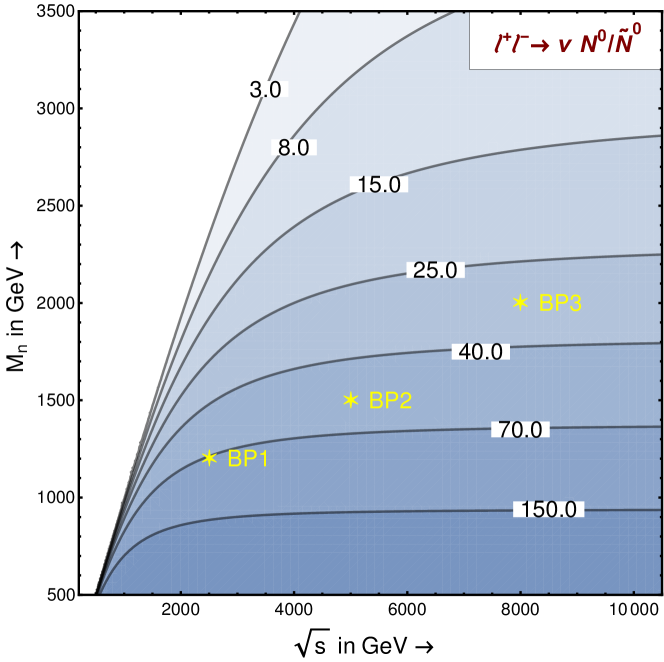
Figure 18: Variation of total cross-section (in fb) for the process $\ell^{+}\ell^{-}\to\nu\,N^{0}/\widetilde{N}^{0}$, with respect to the centre of mass energy and mass of the heavy neutral fermion in the Type-I seesaw scenario ($Y=0.2$, $\mu_{n}=10$ eV). The three benchmark points are represented by the yellow stars.

	$\sigma(\mu^{+}\mu^{-}\to\nu_{\mu}N^{0}/\widetilde{N}^{0})$
Benchmark	$M_{n}$	$E_{CM}$	Cross-section
Points	in GeV	in TeV	(in fb)
BP1	1200	2.5	70.7
BP2	1500	5.0	54.0
BP3	2000	8.0	31.3

Table 5: Masses corresponding to different benchmark points, energy of collision in CM frame and the hard scattering cross-sections (in fb) for $\nu_{\mu}N^{0}/\widetilde{N}^{0}$ final states in Type-I seesaw model and $\mu^{+}\mu^{-}$ collider. ($Y=0.2$, $\mu=10$ eV)

         

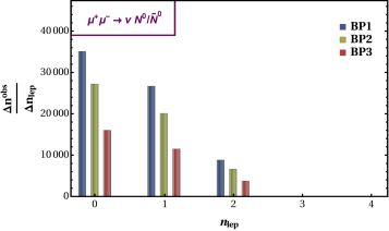
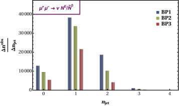
Figure 19: Multiplicity distributions, (a) for the charged leptons ($n_{\rm lep}$) and (b) for the jets ($n_{\rm jet}$) for the benchmark points at the centre of mass energies of 2.5, 5.0, 8.0  TeV, respectively with the integrated luminosity of 1000 fb^-1.

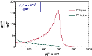
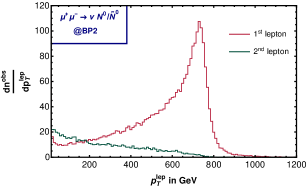
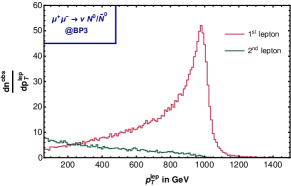
Figure 20: Transverse momentum distribution of the $1^{\rm st}$ and $2^{\rm nd}$ charged leptons ($p_{T}^{\rm lep}$), (a) BP1, (b) BP2 and (c) BP3 at the centre of mass energies of 2.5, 5.0, 8.0  TeV, respectively with the integrated luminosity of 1000 fb^-1.

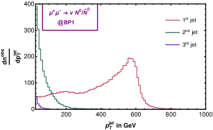
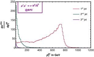
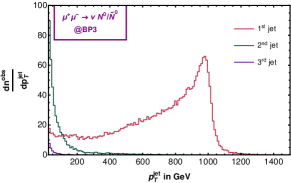
Figure 21: Transverse momentum distribution of the first three $p_{T}$ ordered jets ($p_{T}^{\rm jet}$), (a) BP1, (b) BP2 and (c) BP3 at the centre of mass energies of 2.5, 5.0, 8.0  TeV, respectively with the integrated luminosity of 1000 fb^-1.

It is important to mention here that only one flavour of $\nu$, $N^{0}$ and $\widetilde{N}^{0}$ will be produced during this process since we have assumed diagonal couplings only. However, observation of this mode does not necessarily indicate the existence of Type-I seesaw (inverse) since Type-III seesaw (inverse) also exhibits same signature due to the presence of heavy neutrinos. Therefore, detection of this mode along with non-observation of the $\ell^{\pm}N^{\pm}$ modes, described in subsection 6.3, which is a typicality of Type-III seesaw, will confirm the presence of Type-I seesaw mechanism. It is also noteworthy that although the pair production of these heavy neutrinos can also provide signatures for Type-I and Type-III seesaws, the cross section in that case will be very low due to less available phase space as explained earlier.

For the purpose of simulation, we have considered three different values of $M_{n}$, which are 1.2 TeV, 1.5 TeV and 2.0 TeV respectively, for the three benchmark points. Taking the Yukawa coupling $Y$ to be 0.2 (along with $\mu_{n}=10$ eV) we tabulate the cross-sections of this process at muonic collider for the three benchmark points in Table 5, which are 70.7 fb, 54.0 fb and 31.3 fb, respectively.

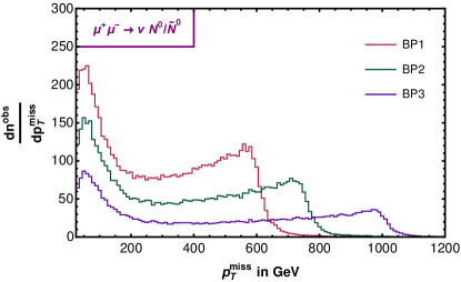
Figure 22: Missing transverse momentum distribution ($p_{T}^{\rm miss}$) for the benchmark points at the centre of mass energies of 1.5, 2.0, 3.0  TeV, respectively with the integrated luminosity of 1000 fb^-1.

Let us now look into the kinematic distributions for this process. The produced heavy neutrino $N^{0}/\widetilde{N}^{0}$ will eventually decay to $W^{\pm}\ell^{\mp}$, $Z\nu$ or $h\nu$ and the decay rates to these channels are given by Equation 6 and Equation 20, which means that the $W^{\pm}\ell^{\mp}$ will have 50% branching ratio while $Z\nu$ and $h\nu$ modes have 25% branching fraction each. Again, $W$-boson has 67% and 33% branching to hadronic and leptonic decay channels respectively whereas $Z$-boson has 69%, 21% and 10% branching to hadronic, invisible and charged leptonic modes. Similarly, the Higgs boson decays to di-quark, di-boson and di-tau channels with 67%, 26% and 7% branching respectively. Therefore, we get multi-jet and multi-lepton signature in the finalstate. The lepton and jet multiplicity for this mode are displayed in left and right panels of Figure 19. If the produced heavy neutrino decays to $Z$ and $h$, and they further decay hadronically then we have two jets with no charged lepton (plus missing energy) in the finalstate. Similarly, if $N^{0}/\widetilde{N}^{0}$ decays to $W$ boson and it further decays hadronically, we get mono-lepton plus di-jet (with missing energy) signature at final state. If the $Z/W$-boson decays leptonically, then only we get di-lepton as can be seen from Figure 19(a). Again the two jets coming from decay of $W$ or $Z$ or $h$ will be highly boosted and hence they might appear as one fatjet which explains the jet multiplicity one finalstates in Figure 19(b).

  

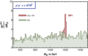
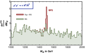
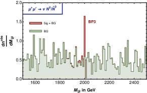
Figure 23: Di-jet-mono-lepton invariant mass distribution ($M_{jjl}$) for (a) BP1, (b) BP2 and (c) BP3 at the centre of mass energies of 2.5, 5.0, 8.0  TeV, respectively with the integrated luminosity of 1000 fb^-1. The total (signal $+$ SM background) signature is depicted in brown and the SM background is in olive green.

	Final states	Signal	Backgrounds
			$t\bar{t}$	$VV$	$VVV$	$t\bar{t}V$	$\ell^{\pm}W^{\mp}\overset{\textbf{(--)}}{\nu}$	$\tau^{+}\tau^{-}$	$\tau^{\pm}W^{\mp}\overset{\textbf{(--)}}{\nu}$	$\tau^{+}\tau^{-}Z$
BP1	$1\ell+2j+p_{T}^{\rm miss}\geq 350\,\rm GeV$	157.10	514.32	1571.45	300.93	6.43	1727.17	163.00	9.96	17.13
	$+|M_{jj\ell}-M_{n}|\leq 10\,$GeV	82.89	0.00	7.40	0.08	0.00	22.63	0.03	0.07	0.00
	Total	82.89	30.21
	$\rm{S}_{\text{sig}}(\mathcal{L}_{\rm int}=1000\,\rm fb^{-1})$	7.79
	$\int\mathcal{L}_{5\sigma}\,[\rm{fb}^{-1}]$	411.97
BP2	$1\ell+2j+p_{T}^{\rm miss}\geq 350\,\rm GeV$	117.46	48.94	885.81	490.88	4.20	4548.38	85.67	6.84	19.73
	$+|M_{jj\ell}-M_{n}|\leq 10\,$GeV	51.85	0.00	1.30	0.02	0.00	34.95	0.00	0.03	0.00
	Total	51.85	36.30
	$\rm{S}_{\text{sig}}(\mathcal{L}_{\rm int}=1000\,\rm fb^{-1})$	5.52
	$\int\mathcal{L}_{5\sigma}\,[\rm{fb}^{-1}]$	820.47
BP3	$1\ell+2j+p_{T}^{\rm miss}\geq 350\,\rm GeV$	50.22	7.34	539.33	421.35	1.80	6615.88	44.50	4.00	13.77
	$+|M_{jj\ell}-M_{n}|\leq 10\,$GeV	15.36	0.00	0.51	0.02	0.00	32.67	0.00	0.01	0.00
	Total	15.36	33.21
	$\rm{S}_{\text{sig}}(\mathcal{L}_{\rm int}=1000\,\rm fb^{-1})$	2.20
	$\int\mathcal{L}_{5\sigma}\,[\rm{fb}^{-1}]$	5165.29

Table 6: Number of events for signal and background corresponding to $1\ell+2j+p_{T}^{\rm miss}\geq 350\,$GeV final state for the benchmark points mentioned in Table 5 with the integrated luminosity of 1000 fb^-1.

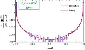
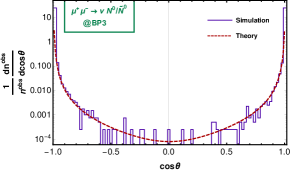
Figure 24: Angular distribution of the reconstructed heavy neutral lepton from $M_{jj\ell}$ invariant mass for (a) BP1, (b) BP2 and (c) BP3 at the centre of mass energies of 2.5, 5.0, 8.0  TeV, respectively. The blue histograms depict the simulated result and the red dashed lines signify the theoretical estimation.

In Figure 20, we represent the transverse momentum distribution of lepton for the process $\mu^{+}\mu^{-}\to\nu_{\mu}N^{0}/\widetilde{N}^{0}$. The left, middle and right panels illustrate this distribution for the three benchmark points, respectively. In this leptonic collider the $\nu_{\mu}N^{0}/\widetilde{N}^{0}$ are produced back to back in the CM frame, this results the light neutrino ($\nu_{\mu}$) and the heavy neutrino ($N^{0}/\widetilde{N}^{0}$) having equal momentum as

$$|\vec{P}_{\nu_{\mu}}|=|\vec{P}_{N^{0}/\widetilde{N}^{0}}|=\frac{s-M_{n}^{2}}{2\sqrt{s}}.$$ (28)

Since, one particle is heavy and another is lighter, energy of the two particles will be different, which can be depicted from the following equation,

$$E_{\nu_{\mu}}=|\vec{P}_{\nu_{\mu}}|\quad\text{and }\quad E_{N^{0}/\widetilde{N}^{0}}=\sqrt{|\vec{P}_{N^{0}/\widetilde{N}^{0}}|^{2}+M_{n}^{2}}.$$ (29)

For the dominant on-shell decays of $N^{0}/\widetilde{N}^{0}\to\ell^{\pm}W^{\mp}$ the momentum is shared between the $\ell^{\pm}$ (red) and $W^{\pm}$ almost equally, resulting the charged lepton $p_{T}$ around half of $M_{n}$. The long tail of the lepton $p_{T}$ can be attributed to the boost of $N^{0}/\widetilde{N}^{0}$. The source of the second lepton (green) is from $W^{\pm}$ and has the usual pattern.

Similarly, Figure 21 depicts the transverse momentum distribution of jets for the benchmark points. The main source of the jets are $W^{\pm},\,Z,\,h$. When those jets are boosted forming a fatjet, they tend to peak around the momentum of $W^{\pm},\,Z,\,h$, which is $M_{n}/2$. However, when the jets are isolated then they follow the usual patter of the jets coming from $W^{\pm},\,Z,\,h$ bosons, having much lower $p_{T}$. The third jet can be attributed to the FSR effect.

Figure 22 depicts the missing energy distributions for the benchmark points. As the collisions happen in CM frame we expect the light neutrino and heavy neutrino should take the equal momentum as shown in Equation 28 and thus expect the $p_{T}^{\rm miss}$ maximum at $|\vec{P}_{\nu_{\mu}}|$, for completely visible decay of $N^{0}/\widetilde{N}^{0}$. However, this is not completely true as 50% of the time $N^{0}/\widetilde{N}^{0}$ decay into $h\nu,\,Z\nu$, causing a missing energy cancellation resulting the peak around $M_{n}/2$. Whereas, the lower end of the $p_{T}^{\rm miss}$ curve occurs when $N^{0}/\widetilde{N}^{0}$ decays into complete invisible sector and missing energy cancels.

Now, to reconstruct the heavy neutrino, we use its $W^{\pm}\ell$ decay mode since the presence of neutrino in the other decay channels will make the reconstruction impossible. Hence, we depict the invariant mass distribution of the di-jet plus mono-lepton combination for all the benchmark points in Figure 23, where the olive green regions indicate the dominant SM background and the brown portions signify the signal plus background. As can be observed, signal plus background show peaks at the corresponding values for mass of the heavy neutrinos.

For signal-background analysis, we look for $1\ell+2j+p_{T}^{\rm miss}\geq 350\,\rm GeV$ finalstate at the $\mu^{+}\mu^{-}$ collider. Since the signal mode occurs through $W$-mediated t-channel diagrams, it is expected that there will be more events in the longitudinal direction (i.e. along the beam axis) than the transverse direction. But various SM backgrounds also grow vigorously near the collinear direction of the beam axis. Therefore, to reduce the background over signal, we focus mainly in the central region with low $|\eta|$ by choosing $p_{T}^{\rm miss}\geq 350$ GeV. Additionally, phase space cut of $\hat{p}_{T}^{\rm min}\geq$ 350 GeV has been implemented while generating the hard process for both signal and background. The analysis for finalstate, mentioned above, with integrated luminosity of 1000 fb^-1 has been displayed in Table 6. The dominant SM backgrounds in this case are $\ell^{\pm}W^{\mp}\overset{\textbf{(--)}}{\nu}$ and di-boson, which decrease significantly after applying the invariant mass cut of $|M_{jjl}-M_{n}|\leq 10$ GeV. The results for BP1 and BP2 are very encouraging since signal significances of 7.8$\sigma$ and $5.5\sigma$ with the integrated luminosity of 1000 fb^-1, respectively. A $5\sigma$ signal significance can be achieved at an integrated luminosities of $\leavevmode\nobreak\ 400$ fb^-1 and $\leavevmode\nobreak\ 800$ fb^-1, respectively. For BP3 we obtain only 2.2$\sigma$ significance with 1000 fb^-1 of luminosity, which means that luminosity of $\sim 5200$ fb^-1 will be needed for $5\sigma$ reach. But this requirement does not lie in the unreachable region of muon collider since $10^{4}$ fb^-1 of integrated luminosity can be achieved around the centre of mass energy of 10 TeV.

Finally, we reconstruct the heavy neutrino $N^{0}/\widetilde{N}^{0}$ from the combination of di-jet plus mono-lepton and depict its angular distribution (with respect to its angle with beam axis) in Figure 24. The three benchmark points have been shown in the three panels respectively where the blue lines represents the simulated results and the red dashed curves signify the theoretical estimates. We find a tub like distribution for this process indicating more number of events along the beam axis and less number of events in the transverse direction of the beam axis.

6.2 Type-II seesaw

Figure 25: Feynman diagrams for $\ell^{+}\ell^{-}\to\Delta^{++}\Delta^{--}$

Next, we scrutinize the possibility of detecting Type-II seesaw at $\ell^{+}\ell^{-}$ collider. For this purpose, we look into the channel of pair production of doubly charged scalar, which is a typicality of Type-II seesaw. The Feynman diagrams for this process are displayed in Figure 25. It can occur through photon and $Z$ mediated s-channel process or lepton mediated t-channel diagram.

The differential and the total cross-sections are given below,

$$\frac{d\sigma}{dx}(\ell^{+}\ell^{-}\to\Delta^{++}\Delta^{--})$$

$$=\frac{\beta^{3}(1-x^{2})}{512\pi sS_{w}^{4}C_{w}^{4}(1-\epsilon_{z})^{2}(1+\beta x-2\epsilon_{\Delta})^{2}}$$

$$\times\bigg{[}e^{4}\Big{\{}4\epsilon_{\Delta}^{2}-4\epsilon_{\Delta}(1+\beta x+x^{2})+(1+2\beta x+x^{2})\Big{\}}$$

$$\times\Big{\{}32\epsilon_{z}^{2}S_{w}^{4}C_{w}^{4}-8\epsilon_{z}C_{w}^{2}S_{w}^{2}(1+2S_{w}^{2})+(1+4S_{w}^{4})\Big{\}}$$

$$-4e^{2}Y_{\Delta}^{2}S_{w}^{2}C_{w}^{2}(1+\beta x-2\epsilon_{\Delta})\Big{\{}1+4\epsilon_{z}^{2}S_{w}^{2}C_{w}^{2}$$

$$-\epsilon_{z}(1+4S_{w}^{2}-4S_{w}^{4})\Big{\}}+4Y_{\Delta}^{4}S_{w}^{4}C_{w}^{4}(1-\epsilon_{z})^{2}\bigg{]}$$ (30)

$$\sigma(\ell^{+}\ell^{-}\to\Delta^{++}\Delta^{--})=\frac{1}{384\pi sS_{w}^{4}C_{w}^{4}(1-\epsilon_{z})^{2}}$$

$$\bigg{[}-\beta\Big{\{}12Y_{\Delta}^{4}S_{w}^{4}C_{w}^{4}(1-\epsilon_{z})^{2}-e^{4}\beta^{2}\Big{(}1-8S_{w}^{2}\epsilon_{z}$$

$$+4S_{w}^{4}\Big{(}1+2\epsilon_{z}(-1+2S_{w}^{2}+4\epsilon_{z}C_{w}^{4})\Big{)}\Big{)}$$

$$+6e^{2}Y_{\Delta}^{2}S_{w}^{2}C_{w}^{2}(1-\epsilon_{z})(1-2\epsilon_{\Delta})(1-4\epsilon_{z}C_{w}^{2}S_{w}^{2})\Big{\}}$$

$$+12Y_{\Delta}^{2}S_{w}^{2}C_{w}^{2}(1-\epsilon_{z})\Big{\{}Y_{\Delta}^{2}S_{w}^{2}C_{w}^{2}(1-\epsilon_{z})(1-2\epsilon_{\Delta})$$

$$+2e^{2}\epsilon_{\Delta}^{2}(1-4\epsilon_{z}S_{w}^{2}C_{w}^{2})\Big{\}}\coth^{-1}\bigg{(}\frac{1-2\epsilon_{\Delta}}{\beta}\bigg{)}\bigg{]},$$ (31)

where, $C_{w}$ and $S_{w}$ are the cosine and sine of the Weinberg angle, respectively, $\epsilon_{\Delta}=M_{\Delta}^{2}/s$, $\epsilon_{z}=m_{Z}^{2}/s$, $\beta=\sqrt{1-4M_{\Delta}^{2}/s}$, $x$ is the cosine of the angle of doubly charged particle with the beam axis and $e$ is the electric charge of the positron.

In Figure 26 we describe the contours of the different values of cross-sections in $M_{\Delta}-\sqrt{s}$ plane. The darker to lighter blue regions depict from higher to lower values of cross-sections. The benchmark points for the collider simulations as summarised in Table 7 are shown by yellow stars.

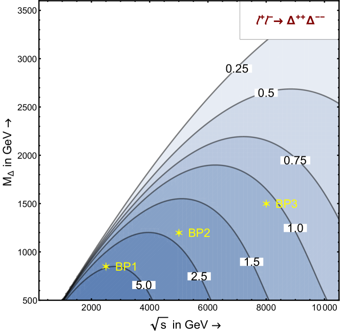
Figure 26: Variation of total cross-section (in fb) for the process $\ell^{+}\ell^{-}\to\Delta^{++}\Delta^{--}$, with respect to the centre of mass energy and mass of the doubly charged scalar in the Type-II seesaw scenario ($Y_{\Delta}=0.2$, $\mu_{\Delta}=10$ eV). The three benchmark points are represented by the yellow stars.

	$\sigma(\mu^{+}\mu^{-}\to\Delta^{++}\Delta^{--})$
Benchmark	$M_{\Delta}$	$E_{CM}$	Cross-section
Points	in GeV	in TeV	(in fb)
BP1	850	2.5	4.8
BP2	1200	5.0	2.2
BP3	1500	8.0	1.1

Table 7: Masses corresponding to different benchmark points, energy of collision in CM frame and the hard scattering cross-sections (in fb) for $\Delta^{++}\Delta^{--}$ final states in Type-II seesaw model and $\mu^{+}\mu^{-}$ collider. ($Y_{\Delta}=0.2$, $\mu_{\Delta}=10$ eV)

For our simulation, we considered three benchmark points with $M_{\Delta}$ being 0.85 TeV, 1.2 TeV and 1.5 TeV, respectively with the centre of mass energy equals to 2.5 TeV, 5.0 TeV and 8.0 TeV,respectively. Assuming $Y_{\Delta}=0.2$ and $\mu_{\Delta}=10$ eV, we find the hard scattering cross-sections for the process $\mu^{+}\mu^{-}\to\Delta^{++}\Delta^{--}$ are 4.8 fb, 2.2 fb and 1.1 fb, respectively and they have been listed in Table 7. Each of these doubly charged scalar will ultimately decay to same sign di-lepton with 33.33% branching fraction to each of the lepton family. Therefore, we search for $2\ell^{+}+2\ell^{-}$ signature at the $\ell^{+}\ell^{-}$ collider in order to identify Type-II seesaw. Here the choice of $v_{\Delta}=10$ eV, makes the $W^{\pm}W^{\pm}$ mode negligible. At this point it is important to mention that one can also try to detect $\Delta^{+}\Delta^{-}$ channel for the same purpose. But, pair production cross-section for single charged scalar is sufficiently lower than $\Delta^{\pm\pm}$ mainly due to smaller electromagnetic charge. Additionally, since $\Delta^{-}$ will decay to one charged lepton and one neutrino, reconstruction of this particle from the finalstate is not possible. On the other hand, pair production of $\Delta^{0}$ is also not possible as this particle does not couple to photon, $Z$ and charged leptons. One can also search for enhancement in $\mu^{+}\mu^{-}\to\mu^{+}\mu^{-}$ due to $\Delta^{++}$ mediated t-channel diagram, but the SM background in this case will be very large. Thus $\mu^{+}\mu^{-}\to\Delta^{++}\Delta^{--}$ seems to be the best mode for searching the trace of Type-II seesaw.

         

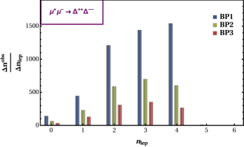
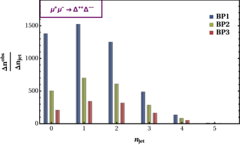
Figure 27: Multiplicity distributions, (a) for the charged leptons ($n_{\rm lep}$) and (b) for the jets ($n_{\rm jet}$) for the benchmark points at the centre of mass energies of 2.5, 5.0, 8.0  TeV, respectively with the integrated luminosity of 1000 fb^-1.

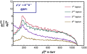
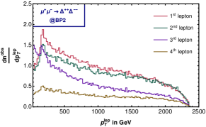
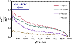
Figure 28: Transverse momentum distributions of the four charged leptons ($p_{T}^{\rm lep}$) coming from $\Delta^{\pm\pm}$ decay, (a) BP1, (b) BP2 and (c) BP3 at the centre of mass energies of 2.5, 5.0, 8.0  TeV, respectively with the integrated luminosity of 1000 fb^-1.

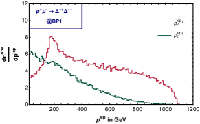
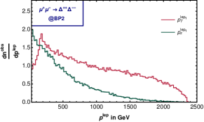
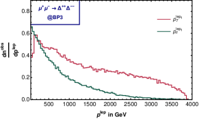
Figure 29: The transverse ($p_{T}^{\rm lep}$ in red) and the longitudinal ($p_{z}^{\rm lep}$ in green) momentum distribution of the $1^{\rm st}$ charged lepton, (a) BP1, (b) BP2 and (c) BP3 at the centre of mass energies of 2.5, 5.0, 8.0  TeV, respectively with the integrated luminosity of 1000 fb^-1.

The doubly charged scalar will eventually decay to same sign di-leptons with equal probability in each of the generations. But if the $\Delta^{--}$ decays to two $\tau$-leptons then we can have jets also in the finalstate from the hadronic decays of $\tau$. In Figure 27, we depict the charged lepton multiplicity (a) and jet multiplicity (b) for this process. The blue, green and red columns indicate the three benchmark points, respectively. The maximum lepton multiplicity is four for all the benchmark points. However, only for BP1, we see that lepton multiplicty peaks around four and for the rest of the benchmark points, it peaks around three due to larger boost effect. Lower multiplicities are attributed to one or more $\Delta^{\pm\pm}$ decays to $\tau$ and the further hadronic decay of the $\tau$. The $\tau$-jet-lepton isolation is also instrumental in reducing the lepton multiplicity further. Figure 27(b) depicts the corresponding the jet-multiplicity distributions, where the jets are coming from the hadronic decays of $\tau$. However, the jets are collimated due to large boost and thus distributions peak at one for all benchmark point.

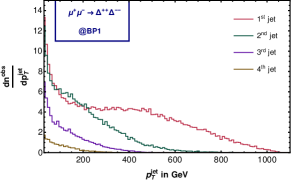
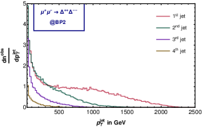
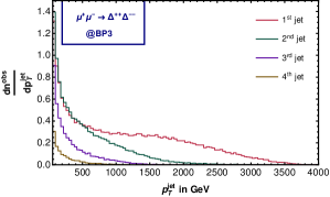
Figure 30: Transverse momentum distributions of the first three $p_{T}$ ordered jets ($p_{T}^{\rm jet}$), (a) BP1, (b) BP2 and (c) BP3 at the centre of mass energies of 2.5, 5.0, 8.0 TeV, respectively with the integrated luminosity of 1000 fb^-1.

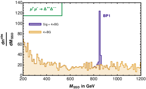
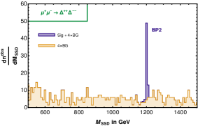
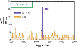
Figure 31: Same sign di-lepton invariant mass distribution ($M_{\rm SSD}$) for (a) BP1, (b) BP2 and (c) BP3 at the centre of mass energies of 2.5, 5.0, 8.0 TeV, respectively with the integrated luminosity of 1000 fb^-1. The total (signal $+$ SM background scaled by 4) signature is depicted in blue and the SM background (scaled by 4) is in yellow.

	Final states	Signal	Backgrounds
			$t\bar{t}$	$VV$	$VVV$	$t\bar{t}V$	$\ell^{+}\ell^{-}Z$	$\tau^{+}\tau^{-}Z$
BP1	$2\ell^{+}+2\ell^{-}$	1530.9	0.2	153.1	133.7	3.5	13855.6	17.4
	$+|M_{\ell\ell}-M_{\Delta}|\leq 10\,$GeV	1491.2	0.0	2.8	2.4	0.0	160.7	0.3
	Total	1491.2	166.2
	$\rm{S}_{\text{sig}}(\mathcal{L}_{\rm int}=1000\,\rm fb^{-1})$	36.6
	$\int\mathcal{L}_{5\sigma}\,[\rm{fb}^{-1}]$	18.7
BP2	$2\ell^{+}+2\ell^{-}$	607.1	0.0	46.6	66.7	0.6	8753.2	5.4
	$+|M_{\ell\ell}-M_{\Delta}|\leq 10\,$GeV	592.4	0.0	1.3	0.7	0.0	43.8	0.1
	Total	592.4	45.9
	$\rm{S}_{\text{sig}}(\mathcal{L}_{\rm int}=1000\,\rm fb^{-1})$	23.4
	$\int\mathcal{L}_{5\sigma}\,[\rm{fb}^{-1}]$	45.5
BP3	$2\ell^{+}+2\ell^{-}$	258.3	0.0	15.9	44.4	0.1	5436.5	2.3
	$+|M_{\ell\ell}-M_{\Delta}|\leq 10\,$GeV	252.1	0.0	0.2	0.5	0.0	20.3	0.0
	Total	252.1	21.0
	$\rm{S}_{\text{sig}}(\mathcal{L}_{\rm int}=1000\,\rm fb^{-1})$	15.3
	$\int\mathcal{L}_{5\sigma}\,[\rm{fb}^{-1}]$	107.4

Table 8: Number of events for signal and background corresponding to $2\ell^{+}+2\ell^{-}$ final state for the benchmark points mentioned in Table 7 with the integrated luminosity of 1000 fb^-1.

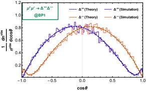
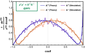
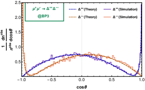
Figure 32: Angular distribution of the reconstructed doubly charged scalar from $M_{\ell\ell}$ invariant mass for (a) BP1, (b) BP2 and (c) BP3 at the centre of mass energies of 2.5, 5.0, 8.0 TeV, respectively. The blue and orange histograms depict the simulated results for positively and negatively charged scalers, respectively, whereas, the blue and orange dashed lines provide their theoretical estimations.

In Figure 28, we show the transverse momentum distributions of the leptons for the mentioned channel, where each panel signifies one benchmark point. Since from the lepton multiplicity distribution we found the maximum number of leptons arising for this mode to be four, we present the $p_{T}^{\rm lep}$ distributions for all the four leptons. The highest energy achievable by each of the leptons in the finalstate is given by:

$$E_{\ell}=\frac{\sqrt{s}}{4}\bigg{(}1+\sqrt{1-\frac{4M_{\Delta}^{2}}{s}}\,\bigg{)},$$ (32)

which, for our the benchmark points, given in Table 7, becomes 1.08 TeV, 2.35 TeV and 3.85 TeV, respectively. Thus we observe the $p_{T}^{\rm lep}$ distributions for all the leptons to vanish at the three mentioned transverse momenta for the three benchmark points. However, as all the the leptons appear from the decay of doubly charged scalars, we do not see any divergence near the endpoint (like Figure 7), rather the distributions gradually reach zero. The behaviour of $p_{z}$ is different from $p_{x}$ and $p_{y}$ at the hard scattering level and $p_{z}$ tends to crossover $p_{x},p_{y}$ at certain value of momentum, towards higher values Sen:2021fha . For $p_{T}$ such crossover happens even at lower values of momentum. This effect though diminished at the decay product level like the charged lepton, but it still exists as can be seen from Figure 29.

In Figure 30, we present the transverse momentum distribution of the jets for all the benchmark points. The red and green curve indicate the hardest and second hardest jets whereas the blue and brown lines signify the other jets. As can be observed, all the distributions peak at very low transverse momentum and diminish gradually with long tails. Figure 31 describes the invariant mass distribution of same sign di-lepton pair for the dominant SM background, shown in yellow, and signal plus background (scaled by four), coloured in blue. Regarding the blue regions, we see clear peaks around the mass of the doubly charged scalar for all the three benchmark points.

Now, we move to signal-background analysis at the muonic collider with an integrated luminosity of 1000 fb^-1, looking for $2\ell^{+}2\ell^{-}$ finalstate. The results are displayed in Table 8, where one can see that the dominant SM background contributing to this final state is $\ell^{+}\ell^{-}Z$. Nevertheless, implication of invariant mass cut as $|M_{\ell\ell}-M_{\Delta}|\leq 10\,$GeV, i.e. the invariant mass of same sign lepton pair should lie within a window of 10 GeV around $M_{\Delta}$, reduces the background drastically. Thus we achieve $36.6\sigma$, $23.4\sigma$ and $15.3\sigma$ of signal significances for the three benchmark points, respectively with the above specified luminosity, which indicates that one can obtain $5\sigma$ of significance with very early data.

Finally, we plot the angular distributions of reconstructed $\Delta^{\pm\pm}$ for the benchmark points with respect to the cosine of their angles with beam axis (taken in the direction of $\mu^{+}$) in CM frame and present them in the three panels of Figure 32. The blue and orange solid histograms indicate the simulated distributions for $\Delta^{++}$ and $\Delta^{--}$, whereas the dashed lines with same colours signify the theoretical estimates for the same. As can be observed, the angular distributions show very unique asymmetric behaviour in this scenario. If we consider the distribution of $\Delta^{++}$ (blue) in BP1 case, we find that it starts with zero at $\cos\theta=-1$ and increases gradually; it reaches the maximum at $\cos\theta\sim-0.15$ and then begins to decrease; finally near $\cos\theta\sim 0.85$, it shows a local minimum and starts to grow again till $\cos\theta=1$. The same patterns repeats for BP2 and BP3 also with only exception of very fast enhancement near $\cos\theta\sim 1$. On the other hand, taking a mirror image of these distributions about $\cos\theta=0$, one can get the angular distributions of $\Delta^{--}$ (orange) for the three benchmark points. Actually, the $\gamma/Z$ mediated s-channel diagram contributes to the angular distribution symmetrically around $\theta=90^{\circ}$, but the t-channel diagram does not. Since, the $\Delta^{++}$ particle can arise from $\ell^{+}$ leg only, we see a divergence in $\cos\theta\sim 1$ direction. Again, the interference terms between s- and t-channel diagrams contribute negatively and for distribution of $\Delta^{++}$ (blue), the negativity increases in $cos\theta>0$ region. Thus combining all these effects, we get such typical asymmetric angular distribution in this scenario.

6.3 Type-III seesaw

Figure 33: Feynman diagrams for $\ell^{+}\ell^{-}\to\ell^{+}N^{-}$

As we have mentioned in subsection 6.1, the observation of the mode $\ell^{+}\ell^{-}\to\nu N^{0}/\widetilde{N}^{0}$ indicates the existence of Type-I or Type-III seesaw; however, it cannot differentiate these two models. In this section, we discuss the litmus test to distinguish these two scenario at $\ell^{+}\ell^{-}$ collider. For this purpose we investigate the channel $\ell^{+}\ell^{-}\to\ell^{\pm}N^{\mp}$. Detection of this mode accompanied by $\nu N^{0}/\widetilde{N}^{0}$ channel will point out the presence of Type-III scenario, whereas, observation of only the second channel will indicate the existence of Type-I case. The relevant Feynman diagrams for the mentioned channel, which are s- and t-channel processes mediated by $Z$ boson, are displayed in Figure 33. However, it is important to mention that the dominant contribution to this mode comes from the t-channel only. The differential distribution and the total cross-section for this channel can be expressed as follows:

$$\frac{d\sigma}{dx}(\ell^{+}\ell^{-}\to\ell^{+}N^{-})=\frac{m_{Z}^{4}Y^{2}\lambda^{2}}{32\pi sv_{0}^{2}M_{n}^{2}}\bigg{[}\frac{16S_{w}^{4}}{(\lambda-\lambda x+2\epsilon_{z})^{2}}$$

$$\hskip 42.67912pt+\frac{(1-2S_{w}^{2})^{2}(1-x^{2})(1-\lambda+\frac{1+x}{1-x})}{(\lambda-\lambda x+2\epsilon_{z})^{2}}\bigg{]},$$ (33)

$$\sigma(\ell^{+}\ell^{-}\to\ell^{+}N^{-})=\frac{m_{Z}^{4}Y^{2}}{16\pi sv_{0}^{2}M_{n}^{2}}\bigg{[}(1-2S_{w}^{2})^{2}\,\Big{(}2\lambda+\frac{\lambda}{\epsilon_{z}}\Big{)}$$

$$+\frac{4\lambda^{2}S_{w}^{4}}{\epsilon_{z}(\lambda+\epsilon_{z})}-(1-2S_{w}^{2})^{2}\,(1+\lambda+2\epsilon_{z})\log\Big{(}1+\frac{\lambda}{\epsilon_{z}}\Big{)}\bigg{]},$$ (34)

with $\epsilon_{z}=m_{Z}^{2}/s$, and $\lambda=(1-M_{n}^{2}/s)$. As stated before, here also $C_{w}$ and $S_{w}$ are the cosine and sine of the Weinberg angle, respectively, $x$ is the cosine of the angle of charged heavy fermion with the beam axis. By charge conjugation symmetry we see that the cross-section is same for $\ell^{+}\ell^{-}\to\ell^{-}N^{+}$ process also. We plot the contours of cross-section in $M_{n}-\sqrt{s}$ plane in Figure 34. The darker to lighter blue regions show higher to lower cross-section regions. The benchmark points detailed in Table 9 are presented by the yellow stars.

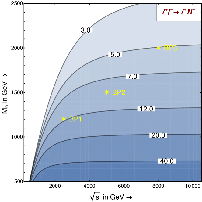
Figure 34: Variation of total cross-section (in fb) for the process $\ell^{+}\ell^{-}\to\ell^{+}N^{-}$, with respect to the centre of mass energy and mass of the charged heavy fermion in the Type-III seesaw scenario ($Y=0.2$, $\mu_{n}=10$ eV). The three benchmark points are represented by the yellow stars.

It is also noteworthy that $\ell^{\pm}\widetilde{N}^{\mp}$ mode cannot be generated at $\ell^{+}\ell^{-}$ collider since $\widetilde{N}^{\mp}$ does not couple to $Z$. For our simulation, we consider three benchmark points taking $M_{n}$ equals to 1.2 TeV, 1.5 TeV and 2.0 TeV along with the centre of mass energy being 2.5 TeV, 5 TeV and 8 TeV respectively at a muonic collider. Assuming $Y=0.2$ and $\mu_{n}=10$ eV, we find the hard scattering cross sections for this channel to be 22.8 fb, 17.5 fb and 10.2 fb respectively which have been presented in Table 9.

	$\sigma(\mu^{+}\mu^{-}\to\mu^{\pm}N^{\mp})$
Benchmark	$M_{n}$	$E_{CM}$	Cross-section
Points	in GeV	in TeV	(in fb)
BP1	1200	2.5	22.8
BP2	1500	5.0	17.5
BP3	2000	8.0	10.2

Table 9: Masses corresponding to different benchmark points, energy of collision in CM frame and the hard scattering cross-sections (in fb) for $\mu^{\pm}N^{\mp}$ final states in Type-III seesaw model and $\mu^{\pm}\mu^{\mp}$ collider. ($Y=0.2$, $\mu=10$ eV)

     

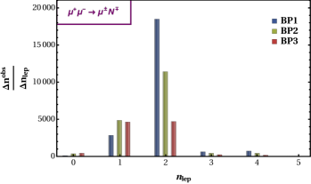
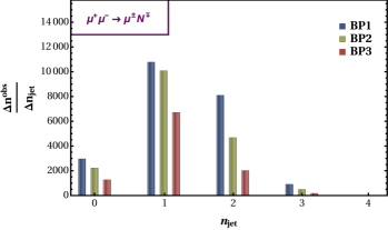
Figure 35: Multiplicity distributions, (a) for the charged leptons ($n_{\rm lep}$) and (b) for the jets ($n_{\rm jet}$) for the benchmark points at the centre of mass energies of 2.5, 5.0, 8.0  TeV, respectively with the integrated luminosity of 1000 fb^-1.

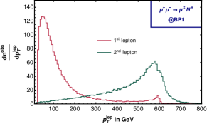
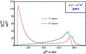
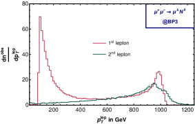
Figure 36: Transverse momentum distributions of the $1^{\rm st}$ and $2^{\rm nd}$ charged leptons ($p_{T}^{\rm lep}$), (a) BP1, (b) BP2 and (c) BP3 at the centre of mass energies of 2.5, 5.0, 8.0  TeV, respectively with the integrated luminosity of 1000 fb^-1.

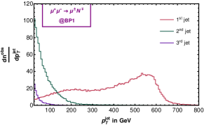
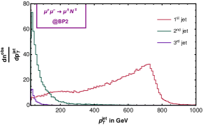
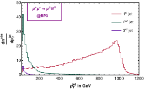
Figure 37: Transverse momentum distribution of the first three $p_{T}$ ordered jets ($p_{T}^{\rm jet}$), (a) BP1, (b) BP2 and (c) BP3 at the centre of mass energies of 2.5, 5.0, 8.0 TeV, respectively with the integrated luminosity of 1000 fb^-1.

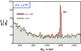
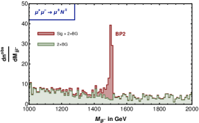
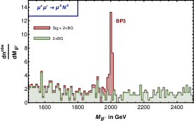
Figure 38: Di-jet-mono-lepton invariant mass distribution ($M_{jjl^{-}}$) for (a) BP1, (b) BP2 and (c) BP3 at the centre of mass energies of 2.5, 5.0, 8.0  TeV, respectively with the integrated luminosity of 1000 fb^-1. The total (signal $+$ SM background scaled by 2) signature is depicted in brown and the SM background (scaled by 2) is in olive green.

Now, we discuss the kinematic distributions of this channel. The multiplicity distributions of charged light leptons and jets are presented in left and right panels of Figure 35. The heavy charged lepton will eventually decay to $Z\ell$ or $h\ell$ and $h/Z$ will disintegrate mostly into two jets. Therefore, we obtain large number of events at lepton number two. On the other hand, for jet multiplicity distribution, we get significant number of events with di-jet. But, since the two jets coming from the decay of $W^{\pm},Z,h$ are highly boosted Sen:2021fha ; Chakraborty:2018khw ; Bhardwaj:2018lma ; CS:TypeI ; Bandyopadhyay:2010ms ; Ashanujjaman:2021zrh ; Ashanujjaman:2022cso , often they are identified as a fatjet and hence large number of events with one jet are found.

The transverse momentum distribution of leptons for the benchmark points are depicted in Figure 36. The red histogram signifies the first lepton which gets produced in association with $N^{\pm}$, while the green histogram symbolizes the second lepton that comes from the decay of $N^{\pm}$. As expected, the green curves peak at half of mass of heavy leptons. The red curves, on the other hand, peak at very low $p_{T}=p\sin{\theta}$, indicating occurrence of large number of events near the beam axis i.e. $\cos{\theta}\sim\pm 1$ as shown in subsection 6.3. On the red curve, we also notice bumps near $M_{n}/2$ which signifies the misidentification of the second lepton as the first one. But, unlike Figure 13, we do not see any additional bump in the red line for the maximum transverse momenta (0.96 TeV, 2.28 TeV and 3.75 TeV, respectively for the benchmark points obtained from Equation 28) by the first lepton as those corresponds to central events around $\eta=0,\,\theta=\frac{\pi}{2}$, where the probability is lowest.

In a similar fashion, the transverse momentum distribution of jets for all the benchmark points are portrayed in Figure 37, where the red curves indicate the hardest jets and remaining green and blue lines signify the other jets. As already mentioned in previous section, the two jets coming from decay of heavy lepton are highly boosted and often provides one fatjet signature. Therefore, we see the red curves also to peak around $M_{n}/2$.

Figure 38 describes the invariant mass distributions for the combination of di-jet plus negatively charged light lepton ($jj\ell^{-}$) concerning all the benchmark points. The SM background (scaled with two) is presented in green while the signal plus background (scaled by two) is shown by red colour. Distinctive peaks in red colour near the heavy lepton mass are clearly visible across all the benchmark scenarios while the background shows more or less flat distributions.

	Final states	Signal	Backgrounds
			$t\bar{t}$	$VV$	$VVV$	$t\bar{t}V$	$\ell^{+}\ell^{-}Z$	$\tau^{+}\tau^{-}Z$
BP1	$\rm{OSD}+2j$	6649.02	132.28	1802.87	1288.43	19.50	93434.50	136.62
	$+|M_{jj\ell}-M_{n}|\leq 10\,$GeV	2480.43	0.06	10.49	4.92	0.00	284.03	1.52
	Total	2480.43	301.02
	$\rm{S}_{\text{sig}}(\mathcal{L}_{\rm int}=1000\,\rm fb^{-1})$	47.03
	$\int\mathcal{L}_{5\sigma}\,[\rm{fb}^{-1}]$	11.30
BP2	$\rm{OSD}+2j$	2741.55	5.47	384.51	638.07	9.58	59532.6	34.67
	$+|M_{jj\ell}-M_{n}|\leq 10\,$GeV	948.52	0.00	0.65	1.52	0.00	61.65	0.19
	Total	948.52	64.01
	$\rm{S}_{\text{sig}}(\mathcal{L}_{\rm int}=1000\,\rm fb^{-1})$	29.81
	$\int\mathcal{L}_{5\sigma}\,[\rm{fb}^{-1}]$	28.14
BP3	$\rm{OSD}+2j$	682.49	0.83	122.73	500.38	4.95	37305.7	11.86
	$+|M_{jj\ell}-M_{n}|\leq 10\,$GeV	205.51	0.00	0.00	0.54	0.00	20.29	0.05
	Total	205.51	20.88
	$\rm{S}_{\text{sig}}(\mathcal{L}_{\rm int}=1000\,\rm fb^{-1})$	13.66
	$\int\mathcal{L}_{5\sigma}\,[\rm{fb}^{-1}]$	134.01

Table 10: Number of events for signal and background corresponding to $\rm{OSD}+2j$ final state for the benchmark points mentioned in Table 9 with the integrated luminosity of 1000 fb^-1.

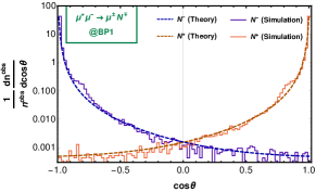
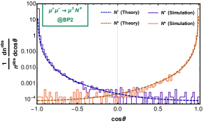
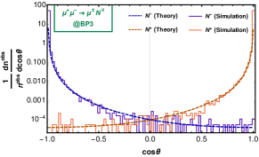
Figure 39: Angular distribution of the reconstructed heavy charged fermion from $M_{jj\ell}$ invariant mass for (a) BP1, (b) BP2 and (c) BP3 at the centre of mass energies of 2.5, 5.0, 8.0  TeV, respectively. The blue and orange histograms depict the simulated results for positively and negatively charged fermion, respectively, whereas, the blue and orange dashed lines provide their theoretical estimations.

The signal-background analysis for this channel is presented in Table 10, where we have scrutinized opposite sign di-lepton (OSD) plus di-jet final state. As can be observed, $\ell^{+}\ell^{-}Z$ provides dominant SM background for this final state. Nonetheless, implementation of invariant mass cut of 10 GeV on the $jj\ell^{-}$ combination around $M_{n}$ reduces the background drastically. Thus, with an integrated luminosity of 1000 fb^-1 we achieved signal significance of 47$\sigma$, $29.8\sigma$ and $13.7\sigma$, respectively for the benchmark points. This indicates that with integrated luminosity of less than 150 fb^-1, one can reach $5\sigma$ significance for this finalstate across all the benchmark points.

Finally, we present the angular distributions of $N^{\pm}$ with respect to the beam axis (taking the $+z$ direction along $\mu^{+}$) for the benchmark points in Figure 39. While the solid blue and red lines illustrate the simulated distributions for $N^{-}$ and $N^{+}$, respectively, the dashed curves represent the same for theoretical estimations. Now, if we concentrate on the blue curves, we see that they diverge at $\cos\theta\sim-1$ and decrease gradually till $\cos\theta\sim 1$. It is expected because more $N^{-}$ will get produced in the same direction of initial state $\mu^{-}$ which travels in the $-z$ direction. On the other hand, the orange curves are the mirror images of the blue one about $\cos\theta=0$. Thus we get a typical asymmetric angular distribution in the Type-III scenario.

It is worth mentioning that one can also look for pair production of heavy charged leptons which are dominated by photon and $Z$ mediated s-channel diagrams. The cross sections for these processes under the chosen benchmark points are also comparable to the numbers presented in Table 9. But the angular distribution of any of the heavy charged lepton will be symmetric about $\cos\theta=0$ Bandyopadhyay:2020wfv .

7 At $\ell^{+}\ell^{\prime-}$ collider

Figure 40: Feynman diagrams for $\ell^{+}\ell^{\prime-}\to\ell^{-}\ell^{\prime+}$

Now, we investigate the prospect of $\ell^{+}\ell^{\prime-}$ collider in discerning the seesaw models. The forthcoming project MUonE is going to look into this kind of collision where a $\mu^{\pm}$ beam of energy $\sim 150$ GeV will be collided with atomic electrons having energy less than 120 GeV to experimentally estimate the hadronic contribution to the muon $(g-2)$ Venanzoni:2019hox ; Masiero:2020vxk . The centre of mass energy and integrated luminosity ($\sim 1.5\times 10^{7}$ nb^-1) of this experiment are too low to search for different BSM scenarios with heavy particles. Therefore, we propose a similar kind of collider with higher centre of mass energy (less than $1$ TeV) and luminosity for the purpose of our study. Since the lower bound on the mass of inverse Type-III seesaw (with three generations) particles is 1.2 TeV (see Figure 2), this model cannot be probed at this collider. For Type-I seesaw there is no such lower bound on the mass of heavy neutrinos, the same $\nu N^{0}/\widetilde{N}^{0}$ mode can be observed if $M_{N^{0}/\widetilde{N}^{0}}<\sqrt{s}$. The cross-section for this process is large and if the flavour of lepton in $1\ell+2j+p_{T}^{\rm miss}$ finalstate is not tagged, the angular distribution of $N^{0}/\widetilde{N}^{0}$ would also look the same as depicted in Figure 24. Therefore, we refrain ourselves from a repetitive analysis and we move to signature of Type-II scenario.

To detect Type-II case, we search the trace of the process $\ell^{+}\ell^{\prime-}\to\ell^{-}\ell^{\prime+}$, i.e. the charges of $\ell$ and $\ell^{\prime}$ get swapped, which occurs through the doubly charged scalar mediated t-channel diagram presented in Figure 40. The angular distribution and the total cross-section for this process is given by

$$\frac{d\sigma}{dx}(\ell^{+}\ell^{\prime-}\to\ell^{-}\ell^{\prime+})=\frac{Y_{\Delta}^{4}}{128\pi s}\frac{(1-x)^{2}}{(1-x+2\epsilon_{\Delta})^{2}}\leavevmode\nobreak\ ,$$ (35)

$$\sigma(\ell^{+}\ell^{\prime-}\to\ell^{-}\ell^{\prime+})=\frac{Y_{\Delta}^{4}}{64\pi s}\bigg{[}\frac{1+2\epsilon_{\Delta}}{1+\epsilon_{\Delta}}-2\epsilon_{\Delta}\log\Big{(}1+\frac{1}{\epsilon_{\Delta}}\Big{)}\bigg{]},$$ (36)

where, $\epsilon_{\Delta}=M_{\Delta}^{2}/s$ and $x$ is the cosine of the angle between $\mu^{+}$ and $\mu^{-}$. In Figure 41 we plots the contours of the cross-sections in $M_{\Delta}-\sqrt{s}$ plane, where the darker to lighter blue regions depict higher to lower values of cross-sections. The benchmark points stated in Table 11 are shown by the yellow stars.

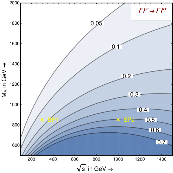
Figure 41: Variation of total cross-section (in fb) for the process $\ell^{+}\ell^{\prime-}\to\ell^{-}\ell^{\prime+}$, with respect to the centre of mass energy and mass of the doubly charged scalar in the Type-II seesaw scenario ($Y_{\Delta}=0.2$, $\mu_{\Delta}=10$ eV). The two benchmark points are represented by the yellow stars.

	$\sigma(\mu^{+}e^{-}\to\mu^{-}e^{+})$
Benchmark	$M_{\Delta}$	$E_{CM}$	Cross-section
Points	in GeV	in GeV	(in fb)
BP1	850	300	0.15
BP2	850	1000	0.51

Table 11: Masses corresponding to different benchmark points, energy of collision in CM frame and the hard scattering cross-sections (in fb) for $\mu^{-}e^{+}$ final states in Type-II seesaw model and $\mu^{+}e^{-}$ collider. ($Y_{\Delta}=0.2$, $\mu_{\Delta}=10$ eV)

         

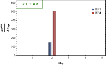
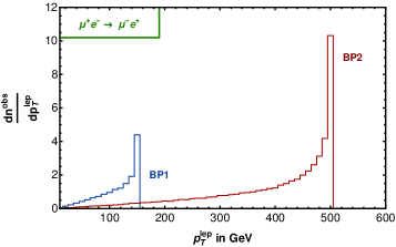
Figure 42: (a) multiplicity distributions for the charged leptons ($n_{\rm lep}$) and (b) their transverse momentum distribution ($p_{T}^{\rm lep}$) for the benchmark points at the centre of mass energies of 300, 1000  GeV, respectively with the integrated luminosity of 1000 fb^-1.

         

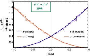
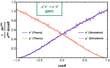
Figure 43: Angular distribution of the finalstate charged leptons ($e^{+}$ in blue and $\mu^{-}$ in orange) for the benchmark points discussed in Table 11. The histogram is for simulated result and the dashed line depicts the theoretical estimation.

For our simulation, we have used $e^{-}$ and $\mu^{+}$ beams with equal energy to collide at a centre of mass energy of 0.3 TeV and 1.0 TeV, respectively, for the two benchmark points. Considering $Y_{\Delta}$ to be 0.2 (with $\mu_{\Delta}=10$ eV) we get the cross-sections for the above mentioned mode to be 0.15 fb and 0.51 fb, respectively, with $M_{\Delta}$ being 0.85 TeV, as presented in Table 11.

In Figure 42, we depict the kinematic distributions for this mode. The left panel exhibits the lepton multiplicity which indicates that there are events with two leptons in the finalstate only, as expected. The right panel demonstrates transverse momentum distributions of leptons which is supposed to diverge at half of the centre of mass energy obeying Equation 23.

Final state	BP1	BP2
$1\mu^{-}1e^{+}$	149.2	508.2

Table 12: Number of events for $1\mu^{-}1e^{+}$ final state with an integrated luminosity of 1000 fb^-1.

Now, we look for $\mu^{-}e^{+}$ final state at the collider. The results for this final state with 1000 fb^-1 of integrated luminosity are presented in Table 12, where we find 149 and 508 numbers of events for the two benchmark points. It is interesting to mention that there is no SM background for this finalstate since this is a lepton flavour violating process.

Finally, we illustrate the angular distributions for the final state leptons in the CM frame with respect to the angle with initial state muon ($\mu^{+}$) beam in Figure 43, where the two benchmark scenarios are shown in the two panels. While the orange curves signify angular distributions for final state $\mu^{-}$, the blue curves indicate the same for final state $e^{+}$. In both the plots the solid lines denote the simulated result whereas the dashed lines demonstrate the theoretical predictions. As can be seen, the blue curves start from zero at $\cos\theta=-1$ and then increase gradually with $\cos\theta$. On the other hand, the orange curves are the mirror image of the blue ones about $\cos\theta=0$ line. It is interesting to notice that the curves representing the angular distributions remain convex in nature at low centre of mass energies (like in BP1); however as the energy of interaction increases, the convexity decreases and at further high energies the curves become concave (like in BP2).

8 Conclusion

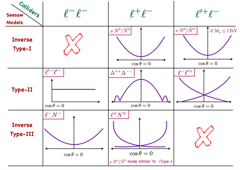
Figure 44: A table of schematic diagrams on the angular distribution at $\ell^{-}\ell^{-}$, $\ell^{+}\ell^{-}$ and $\ell^{\prime+}\ell^{-}$ colliders for inverse Type-I, Type-II and inverse Type-III seesaw models with the detectable modes. This reflects discerning signatures of seesaw models at various leptonic colliders.

In this article, we have tried to separate the signatures of different seesaw scenarios in different leptonic colliders. We show that the angular distributions of the finalstate leptons or reconstructed BSM particles can provide important information about the seesaw models. In our analysis, we have mainly focused on detecting the TeV-scale BSM particles with diagonal coupling of $\mathcal{O}(0.1)$. Since the neutrino mass bound restricts the couplings for Type-I and Type-III seesaw models with TeV-scaled new particles to be very small, these models become very challenging to be probed at colliders. Hence, we choose inverse seesaw scenarios for both Type-I and Type-III cases to be investigated. A detailed PYTHIA based analysis at $\mu^{-}\mu^{-}$, $\mu^{+}\mu^{-}$ and $\mu^{+}e^{-}$ colliders are carried out with different masses and centre of mass energies taking the diagonal couplings for the BSM particles.

The angular distributions which are instrumental in distinguishing such different seesaw scenarios at different leptonic colliders are summarized in Figure 44. It can be clearly seen that $\ell^{+}\ell^{-}$ has an advantage as all the three types of seesaw can be probed and their angular distributions are also different. The $\ell^{-}\ell^{-}$ and $\ell^{\prime\,+}\ell^{-}$ colliders cannot proved the inverse Type-I and inverse Type-III, respectively. However, they able to distinguish the rest of seesaw scenarios.

As high-energetic and highly luminous muon beams are going to be available in near future we have mostly used muonic colliders during our simulation. At $\mu^{-}\mu^{-}$ collider, it is not possible to probe Type-I seesaw (inverse), since lepton number violating $W^{-}W^{-}$ mode is the only channel to be considered in this case and the cross-section for this mode is very small as the lepton number violating parameter $\mu_{n}$ is tiny. For Type-II scenario we searched for the mode $e^{-}e^{-}$, which should show a flat angular distribution of $e^{-}$ in the CM frame. On the contrary, for Type-III case we examined the $\mu^{-}N^{-}$ mode which is expected to display a tub-like angular distribution for the final state muon (or the reconstructed $N^{-}$) in the CM frame.

At $\mu^{+}\mu^{-}$ collider, we first looked for $\nu N^{0}/\widetilde{N}^{0}$ mode. It presents a bowl-like angular distribution for the reconstructed $N^{0}/\widetilde{N}^{0}$. However, both Type-I and Type-III scenarios exhibit same feature for this particular mode. So, in addition to it, one has to investigate the presence or absence of another mode, i.e. $\mu^{\pm}N^{\mp}$, to confirm the existence of anyone of these two models. For Type-III seesaw, this particular mode will exist with a typical asymmetric angular distribution of $\mu^{\pm}$ (or $N^{\pm}$), whereas in Type-I seesaw, this channel does not exist. Regarding Type-II seesaw, we have scrutinized the pair production of doubly charged scalar which displays a very unique asymmetric angular distribution.

Finally, motivated by MUonE project, we investigated the possibilities at low energy muon-electron collider ($\sqrt{s}\leq 1$ TeV) too. Since the mass bound on inverse Type-III seesaw with three generations of triplets is $\sim 1.2$ TeV, one needs to enhance the CM energy to probe the scenario. Since this kind collider bound is not there for Type-I case, one can search for right-handed neutrinos with mass less than 1 TeV through the mode $\nu N^{0}/\widetilde{N}^{0}$, which will show the similar bowl-like angular distribution if the flavour of final state lepton is not tagged. The most interesting feature at this collider is observed for Type-II seesaw when we search the mode $e^{-}\mu^{+}\to e^{+}\mu^{-}$. The angular distribution of finalstate electron or muon exhibit a very distinctive asymmetric behaviour in this case.

Appendix A Decay of $N^{\pm}/\widetilde{N}^{\pm}$ in iType-III model with one generation

Here, we briefly discuss the typical behaviour of iType-III seesaw involving the decay of heavy charged leptons. For simplicity, we show it with one generation of lepton and right handed neutrinos. During the diagonalization of mass matrix, the rotation matrices needed for negatively and positively charged leptons are denoted as $Z^{L}$ and $Z^{R}$ respectively whereas the same for neutral leptons are termed as $U$. Assuming $M_{n}\gg v_{0}Y\gg v_{0}Y_{e}$, where $Y_{e}$ is the Yukawa coupling for SM lepton, these three rotation matrices for iType-III seesaw can be expressed as:

$$Z^{L}\approx\begin{pmatrix}1&0&-\frac{v_{0}Y}{M_{n}}\\ 0&1&0\\ \frac{v_{0}Y}{M_{n}}&0&1\end{pmatrix},Z^{R}\approx\begin{pmatrix}1&0&0\\ 0&0&1\\ 0&1&0\end{pmatrix},$$

$$U\approx\begin{pmatrix}1&0&-\frac{v_{0}Y}{\sqrt{2}M_{n}}\\ \frac{v_{0}Y}{2M_{n}}&-\frac{1}{\sqrt{2}}&\frac{1}{\sqrt{2}}\\ -\frac{v_{0}Y}{2M_{n}}&-\frac{1}{\sqrt{2}}&-\frac{1}{\sqrt{2}}\end{pmatrix}.$$ (37)

Now, the couplings for the vertices involving the decay of the heavy charged leptons in this scenario can be written as:

$$\bar{\nu}_{j}e_{i}W_{\mu}^{+}\equiv-ig_{2}\bigg{[}\Big{(}\frac{1}{\sqrt{2}} U_{j1}Z_{i1}^{L}+U_{j2}Z_{i2}^{L}+U_{j3}Z_{i3}^{L}\Big{)}\gamma_{\mu}\gamma_{L}$$

$$+\Big{(}U_{j2}Z^{R}_{i2}+U_{j3}Z^{R}_{i3}\Big{)}\gamma_{\mu}\gamma_{R}\bigg{]},$$ (38)

$$\bar{e}_{i}e_{j}Z_{\mu} \equiv i\Big{\{}\Big{(}\frac{g_{2}}{2}C_{w}-\frac{g_{1}}{2}S_{w}\Big{)}Z^{L}_{i1}Z^{L}_{j1}+g_{2}C_{w}\Big{(}Z^{L}_{i2}Z^{L}_{j2}$$

$$+Z^{L}_{i3}Z^{L}_{j3}\Big{)}\Big{\}}\gamma_{\mu}\gamma_{L}-i\Big{\{}g_{1}S_{w}Z^{R}_{i1}Z^{R}_{j1}-g_{2}C_{w}\Big{(}Z^{R}_{i2}Z^{R}_{j2}$$

$$+Z^{R}_{i3}Z^{R}_{j3}\Big{)}\Big{\}}\gamma_{\mu}\gamma_{R},$$ (39)

$$\bar{e}_{i}e_{j}h\equiv-iZ^{L}_{j1}\Big{(}\frac{Y_{e}}{\sqrt{2}}Z^{R}_{i1} -YZ^{R}_{i2}\Big{)}\gamma_{L}$$

$$-iZ^{L}_{i1}\Big{(}\frac{Y_{e}}{\sqrt{2}}Z^{R}_{j1}-YZ^{R}_{j2}\Big{)}\gamma_{R},$$ (40)

where $e_{i}=(e^{-},\widetilde{N}^{-},N^{-})$ and $\nu_{j}=(\nu_{e},\widetilde{N}_{0},N^{0})$ for $(i,j)\in\{1,2,3\}$. One can easily check that the couplings for the vertices $\bar{\nu}_{e}N^{-}W_{\mu}^{+}$, $\bar{e}\widetilde{N}^{-}Z_{\mu}$ and $\bar{e}\widetilde{N}^{-}h$ regarding the decay of the heavy charged leptons are zero and the rest of the couplings involving transition of heavy charged leptons to SM leptons are non-zero. Therefore, we find the partial decay widths of $N^{\pm}/\widetilde{N}^{\pm}$ as:

$$\Gamma(N^{-}\to\nu_{e}W^{-})=0,$$ (41)

$$\Gamma({N^{-}}\to{Ze^{-}})=\Gamma({N^{-}}\to{Ze^{-}})=\frac{Y^{2}M_{n}}{32\pi},$$ (42)

$$\Gamma(\widetilde{N}^{-}\to\nu_{e}W^{-})=\frac{Y^{2}M_{n}}{16\pi},$$ (43)

$$\Gamma({\widetilde{N}^{-}}\to{Ze^{-}})=\Gamma({\widetilde{N}^{-}}\to{Ze^{-}})=0.$$ (44)

References

- (1) S.M. Bilenky and S.T. Petcov, Massive Neutrinos and Neutrino Oscillations, Rev. Mod. Phys. 59 (1987) 671.
- (2) Particle Data Group collaboration, Review of Particle Physics, PTEP 2020 (2020) 083C01.
- (3) B. Bajc, M. Nemevsek and G. Senjanovic, Probing seesaw at LHC, Phys. Rev. D 76 (2007) 055011 [hep-ph/0703080].
- (4) F. del Aguila and J.A. Aguilar-Saavedra, Distinguishing seesaw models at LHC with multi-lepton signals, Nucl. Phys. B 813 (2009) 22 [0808.2468].
- (5) F.F. Deppisch, P.S. Bhupal Dev and A. Pilaftsis, Neutrinos and Collider Physics, New J. Phys. 17 (2015) 075019 [1502.06541].
- (6) Y. Cai, T. Han, T. Li and R. Ruiz, Lepton Number Violation: Seesaw Models and Their Collider Tests, Front. in Phys. 6 (2018) 40 [1711.02180].
- (7) P. Fileviez Perez, T. Han, G.-y. Huang, T. Li and K. Wang, Neutrino Masses and the CERN LHC: Testing Type II Seesaw, Phys. Rev. D 78 (2008) 015018 [0805.3536].
- (8) A. Melfo, M. Nemevsek, F. Nesti, G. Senjanovic and Y. Zhang, Type II Seesaw at LHC: The Roadmap, Phys. Rev. D 85 (2012) 055018 [1108.4416].
- (9) R. Franceschini, T. Hambye and A. Strumia, Type-III see-saw at LHC, Phys. Rev. D 78 (2008) 033002 [0805.1613].
- (10) T. Li and X.-G. He, Neutrino Masses and Heavy Triplet Leptons at the LHC: Testability of Type III Seesaw, Phys. Rev. D 80 (2009) 093003 [0907.4193].
- (11) J.A. Aguilar-Saavedra, P.M. Boavida and F.R. Joaquim, Flavored searches for type-III seesaw mechanism at the LHC, Phys. Rev. D 88 (2013) 113008 [1308.3226].
- (12) P. Bandyopadhyay, S. Choi, E.J. Chun and K. Min, Probing Higgs bosons via the type III seesaw mechanism at the LHC, Phys. Rev. D 85 (2012) 073013 [1112.3080].
- (13) ATLAS collaboration, Search for type-III seesaw heavy leptons in dilepton final states in collisions at = 13 TeV with the ATLAS detector, Eur. Phys. J. C 81 (2021) 218 [2008.07949].
- (14) CMS collaboration, Search for Evidence of the Type-III Seesaw Mechanism in Multilepton Final States in Proton-Proton Collisions at , Phys. Rev. Lett. 119 (2017) 221802 [1708.07962].
- (15) CMS collaboration, Search for physics beyond the standard model in multilepton final states in proton-proton collisions at 13 TeV, JHEP 03 (2020) 051 [1911.04968].
- (16) D. Goswami and P. Poulose, Direct searches of Type III seesaw triplet fermions at high energy collider, Eur. Phys. J. C 78 (2018) 42 [1702.07215].
- (17) A. Das and N. Okada, Inverse seesaw neutrino signatures at the LHC and ILC, Phys. Rev. D 88 (2013) 113001 [1207.3734].
- (18) A. Das, S. Jana, S. Mandal and S. Nandi, Probing right handed neutrinos at the LHeC and lepton colliders using fat jet signatures, Phys. Rev. D 99 (2019) 055030 [1811.04291].
- (19) A. Das, S. Mandal and T. Modak, Testing triplet fermions at the electron-positron and electron-proton colliders using fat jet signatures, Phys. Rev. D 102 (2020) 033001 [2005.02267].
- (20) P. Bandyopadhyay, E.J. Chun, H. Okada and J.-C. Park, Higgs Signatures in Inverse Seesaw Model at the LHC, JHEP 01 (2013) 079 [1209.4803].
- (21) P. Bandyopadhyay and E.J. Chun, Lepton flavour violating signature in supersymmetric seesaw models at the LHC, JHEP 05 (2015) 045 [1412.7312].
- (22) P. Bandyopadhyay, E.J. Chun and J.-C. Park, Right-handed sneutrino dark matter in seesaw models and its signatures at the LHC, JHEP 06 (2011) 129 [1105.1652].
- (23) P. Bandyopadhyay, Displaced lepton flavour violating signatures of right-handed sneutrinos in supersymmetric models, JHEP 09 (2017) 052 [1511.03842].
- (24) A. Atre, T. Han, S. Pascoli and B. Zhang, The Search for Heavy Majorana Neutrinos, JHEP 05 (2009) 030 [0901.3589].
- (25) C.A. Heusch, Linear electron-electron colliders, AIP Conference Proceedings 397 (1997) 235 [https://aip.scitation.org/doi/pdf/10.1063/1.52996].
- (26) N. Arkani-Hamed, H.-C. Cheng, J.L. Feng and L.J. Hall, Probing lepton flavor violation at future colliders, Phys. Rev. Lett. 77 (1996) 1937 [hep-ph/9603431].
- (27) J.L. Feng, Lepton flavor violation at LEP-2 and beyond, Nucl. Phys. B Proc. Suppl. 52 (1997) 100 [hep-ph/9607453].
- (28) J.L. Feng, Physics at e-e- colliders, Int. J. Mod. Phys. A 15 (2000) 2355 [hep-ph/0002055].
- (29) A. De Roeck, Physics at a and option for a linear collider, in 4th ECFA / DESY Workshop on Physics and Detectors for a 90-GeV to 800-GeV Linear e+ e- Collider, pp. 69–78, 11, 2003 [hep-ph/0311138].
- (30) C. Heusch, The search for new physics phenomena using e-e- collisions in the clic energy range, International Journal of Modern Physics A - IJMPA 20 (2005) 7338.
- (31) W. Rodejohann and H. Zhang, Higgs triplets at like-sign linear colliders and neutrino mixing, Phys. Rev. D 83 (2011) 073005 [1011.3606].
- (32) A. Datta, K. Kong and K.T. Matchev, Discrimination of supersymmetry and universal extra dimensions at hadron colliders, Phys. Rev. D 72 (2005) 096006 [hep-ph/0509246].
- (33) M. Battaglia, A.K. Datta, A. De Roeck, K. Kong and K.T. Matchev, Contrasting supersymmetry and universal extra dimensions at colliders, eConf C050318 (2005) 0302 [hep-ph/0507284].
- (34) N.D. Christensen, P. de Aquino, N. Deutschmann, C. Duhr, B. Fuks, C. Garcia-Cely et al., Simulating spin- particles at colliders, Eur. Phys. J. C 73 (2013) 2580 [1308.1668].
- (35) P. Bandyopadhyay, S. Dutta and A. Karan, Zeros of amplitude in the associated production of photon and leptoquark at collider, Eur. Phys. J. C 81 (2021) 315 [2012.13644].
- (36) P. Bandyopadhyay, S. Dutta and A. Karan, Investigating the Production of Leptoquarks by Means of Zeros of Amplitude at Photon Electron Collider, Eur. Phys. J. C 80 (2020) 573 [2003.11751].
- (37) P. Bandyopadhyay, S. Dutta, M. Jakkapu and A. Karan, Distinguishing Leptoquarks at the LHC/FCC, Nucl. Phys. B 971 (2021) 115524 [2007.12997].
- (38) P. Minkowski, at a Rate of One Out of Muon Decays?, Phys. Lett. B 67 (1977) 421.
- (39) T. Yanagida, Horizontal gauge symmetry and masses of neutrinos, Conf. Proc. C 7902131 (1979) 95.
- (40) M. Gell-Mann, P. Ramond and R. Slansky, Complex Spinors and Unified Theories, Conf. Proc. C 790927 (1979) 315 [1306.4669].
- (41) S.L. Glashow, The Future of Elementary Particle Physics, NATO Sci. Ser. B 61 (1980) 687.
- (42) R.N. Mohapatra and G. Senjanović, Neutrino mass and spontaneous parity nonconservation, Phys. Rev. Lett. 44 (1980) 912.
- (43) R.N. Mohapatra, Mechanism for Understanding Small Neutrino Mass in Superstring Theories, Phys. Rev. Lett. 56 (1986) 561.
- (44) S. Nandi and U. Sarkar, A Solution to the Neutrino Mass Problem in Superstring E6 Theory, Phys. Rev. Lett. 56 (1986) 564.
- (45) R.N. Mohapatra and J.W.F. Valle, Neutrino mass and baryon-number nonconservation in superstring models, Phys. Rev. D 34 (1986) 1642.
- (46) W. Konetschny and W. Kummer, Nonconservation of Total Lepton Number with Scalar Bosons, Phys. Lett. B 70 (1977) 433.
- (47) J. Schechter and J.W.F. Valle, Neutrino masses in su(2) u(1) theories, Phys. Rev. D 22 (1980) 2227.
- (48) M. Magg and C. Wetterich, Neutrino Mass Problem and Gauge Hierarchy, Phys. Lett. B 94 (1980) 61.
- (49) T.P. Cheng and L.-F. Li, Neutrino Masses, Mixings and Oscillations in SU(2) x U(1) Models of Electroweak Interactions, Phys. Rev. D 22 (1980) 2860.
- (50) G. Lazarides, Q. Shafi and C. Wetterich, Proton Lifetime and Fermion Masses in an SO(10) Model, Nucl. Phys. B 181 (1981) 287.
- (51) R.N. Mohapatra and G. Senjanovic, Neutrino Masses and Mixings in Gauge Models with Spontaneous Parity Violation, Phys. Rev. D 23 (1981) 165.
- (52) C. Wetterich, Neutrino Masses and the Scale of B-L Violation, Nucl. Phys. B 187 (1981) 343.
- (53) G.B. Gelmini and M. Roncadelli, Left-Handed Neutrino Mass Scale and Spontaneously Broken Lepton Number, Phys. Lett. B 99 (1981) 411.
- (54) E.J. Chun and P. Sharma, Search for a doubly-charged boson in four lepton final states in type II seesaw, Phys. Lett. B 728 (2014) 256 [1309.6888].
- (55) CMS collaboration, A search for doubly-charged Higgs boson production in three and four lepton final states at , .
- (56) ATLAS collaboration, Search for doubly charged Higgs boson production in multi-lepton final states with the ATLAS detector using proton–proton collisions at , Eur. Phys. J. C 78 (2018) 199 [1710.09748].
- (57) Particle Data Group collaboration, Review of Particle Physics, PTEP 2020 (2020) 083C01.
- (58) M. Kakizaki, Y. Ogura and F. Shima, Lepton flavor violation in the triplet Higgs model, Phys. Lett. B 566 (2003) 210 [hep-ph/0304254].
- (59) S. Antusch, O. Fischer, A. Hammad and C. Scherb, Low scale type II seesaw: Present constraints and prospects for displaced vertex searches, JHEP 02 (2019) 157 [1811.03476].
- (60) R. Primulando, J. Julio and P. Uttayarat, Scalar phenomenology in type-II seesaw model, JHEP 08 (2019) 024 [1903.02493].
- (61) M. Lindner, M. Platscher and F.S. Queiroz, A Call for New Physics : The Muon Anomalous Magnetic Moment and Lepton Flavor Violation, Phys. Rept. 731 (2018) 1 [1610.06587].
- (62) C. Han, D. Huang, J. Tang and Y. Zhang, Probing the doubly charged Higgs boson with a muonium to antimuonium conversion experiment, Phys. Rev. D 103 (2021) 055023 [2102.00758].
- (63) B. Pontecorvo, Mesonium and anti-mesonium, Sov. Phys. JETP 6 (1957) 429.
- (64) D. Chang and W.-Y. Keung, Constraints on Muonium - anti-Muonium Conversion, Phys. Rev. Lett. 62 (1989) 2583.
- (65) L. Willmann et al., New bounds from searching for muonium to anti-muonium conversion, Phys. Rev. Lett. 82 (1999) 49 [hep-ex/9807011].
- (66) J.T. et al., Search for muonium to antimuonium conversion, Letter of interest contribution to snowmass21 .
- (67) T.E. Clark and S.T. Love, Muonium - anti-muonium oscillations and massive Majorana neutrinos, Mod. Phys. Lett. A 19 (2004) 297 [hep-ph/0307264].
- (68) G. Cvetic, C.O. Dib, C.S. Kim and J.D. Kim, Muonium-antimuonium conversion in models with heavy neutrinos, Phys. Rev. D 71 (2005) 113013 [hep-ph/0504126].
- (69) Muon g-2 collaboration, Measurement of the Positive Muon Anomalous Magnetic Moment to 0.46 ppm, Phys. Rev. Lett. 126 (2021) 141801 [2104.03281].
- (70) R. Foot, H. Lew, X.G. He and G.C. Joshi, Seesaw Neutrino Masses Induced by a Triplet of Leptons, Z. Phys. C 44 (1989) 441.
- (71) E. Ma, Pathways to naturally small neutrino masses, Phys. Rev. Lett. 81 (1998) 1171 [hep-ph/9805219].
- (72) E. Ma and D.P. Roy, Heavy triplet leptons and new gauge boson, Nucl. Phys. B 644 (2002) 290 [hep-ph/0206150].
- (73) T. Hambye, Y. Lin, A. Notari, M. Papucci and A. Strumia, Constraints on neutrino masses from leptogenesis models, Nucl. Phys. B 695 (2004) 169 [hep-ph/0312203].
- (74) A. Abada, C. Biggio, F. Bonnet, M.B. Gavela and T. Hambye, Low energy effects of neutrino masses, JHEP 12 (2007) 061 [0707.4058].
- (75) I. Dorsner and P. Fileviez Perez, Upper Bound on the Mass of the Type III Seesaw Triplet in an SU(5) Model, JHEP 06 (2007) 029 [hep-ph/0612216].
- (76) A. Abada, C. Biggio, F. Bonnet, M.B. Gavela and T. Hambye, mu — e gamma and tau — l gamma decays in the fermion triplet seesaw model, Phys. Rev. D 78 (2008) 033007 [0803.0481].
- (77) X.-G. He and S. Oh, Lepton FCNC in Type III Seesaw Model, JHEP 09 (2009) 027 [0902.4082].
- (78) P. Bandyopadhyay, S. Choubey and M. Mitra, Two Higgs Doublet Type III Seesaw with mu-tau symmetry at LHC, JHEP 10 (2009) 012 [0906.5330].
- (79) P. Bandyopadhyay and E.J. Chun, Displaced Higgs production in type III seesaw, JHEP 11 (2010) 006 [1007.2281].
- (80) M. Cirelli, N. Fornengo and A. Strumia, Minimal dark matter, Nucl. Phys. B 753 (2006) 178 [hep-ph/0512090].
- (81) C. Sen, P. Bandyopadhyay, S. Dutta and A. KT, Displaced Higgs production in Type-III Seesaw at the LHC/FCC, MATHUSLA and Muon collider, 2107.12442.
- (82) E. Ma, Inverse Seesaw Neutrino Mass from Lepton Triplets in the U(1)(Sigma) Model, Mod. Phys. Lett. A 24 (2009) 2491 [0905.2972].
- (83) O.J.P. Eboli, J. Gonzalez-Fraile and M.C. Gonzalez-Garcia, Neutrino Masses at LHC: Minimal Lepton Flavour Violation in Type-III See-saw, JHEP 12 (2011) 009 [1108.0661].
- (84) N.R. Agostinho, O.J.P. Eboli and M.C. Gonzalez-Garcia, LHC Run I Bounds on Minimal Lepton Flavour Violation in Type-III See-saw: A Case Study, JHEP 11 (2017) 118 [1708.08456].
- (85) P. Bandyopadhyay, S. Jangid and M. Mitra, Scrutinizing Vacuum Stability in IDM with Type-III Inverse seesaw, JHEP 02 (2021) 075 [2008.11956].
- (86) S.J. Brodsky and R.W. Brown, Zeros in Amplitudes: Gauge Theory and Radiation Interference, Phys. Rev. Lett. 49 (1982) 966.
- (87) F. Staub, SARAH 4 : A tool for (not only SUSY) model builders, Comput. Phys. Commun. 185 (2014) 1773 [1309.7223].
- (88) A. Belyaev, N.D. Christensen and A. Pukhov, CalcHEP 3.4 for collider physics within and beyond the Standard Model, Comput. Phys. Commun. 184 (2013) 1729 [1207.6082].
- (89) T. Sjostrand, S. Mrenna and P.Z. Skands, A Brief Introduction to PYTHIA 8.1, Comput. Phys. Commun. 178 (2008) 852 [0710.3820].
- (90) T. Sjöstrand, S. Ask, J.R. Christiansen, R. Corke, N. Desai, P. Ilten et al., An introduction to PYTHIA 8.2, Comput. Phys. Commun. 191 (2015) 159 [1410.3012].
- (91) M. Cacciari, G.P. Salam and G. Soyez, FastJet User Manual, Eur. Phys. J. C 72 (2012) 1896 [1111.6097].
- (92) C.M. Ankenbrandt et al., Status of muon collider research and development and future plans, Phys. Rev. ST Accel. Beams 2 (1999) 081001 [physics/9901022].
- (93) J.P. Delahaye, M. Diemoz, K. Long, B. Mansoulié, N. Pastrone, L. Rivkin et al., Muon Colliders, 1901.06150.
- (94) N. Bartosik et al., Preliminary Report on the Study of Beam-Induced Background Effects at a Muon Collider, 1905.03725.
- (95) H. Al Ali et al., The Muon Smasher’s Guide, 2103.14043.
- (96) N. Bartosik et al., Detector and Physics Performance at a Muon Collider, JINST 15 (2020) P05001 [2001.04431].
- (97) A. Costantini, F. De Lillo, F. Maltoni, L. Mantani, O. Mattelaer, R. Ruiz et al., Vector boson fusion at multi-TeV muon colliders, JHEP 09 (2020) 080 [2005.10289].
- (98) D. Buttazzo, D. Redigolo, F. Sala and A. Tesi, Fusing Vectors into Scalars at High Energy Lepton Colliders, JHEP 11 (2018) 144 [1807.04743].
- (99) G.-Y. Huang, S. Jana, F.S. Queiroz and W. Rodejohann, Probing the Anomaly at a Muon Collider, 2103.01617.
- (100) G.-y. Huang, F.S. Queiroz and W. Rodejohann, Gauged at a muon collider, Phys. Rev. D 103 (2021) 095005 [2101.04956].
- (101) P. Asadi, R. Capdevilla, C. Cesarotti and S. Homiller, Searching for Leptoquarks at Future Muon Colliders, 2104.05720.
- (102) R. Capdevilla, D. Curtin, Y. Kahn and G. Krnjaic, Discovering the physics of at future muon colliders, Phys. Rev. D 103 (2021) 075028 [2006.16277].
- (103) R. Capdevilla, D. Curtin, Y. Kahn and G. Krnjaic, A No-Lose Theorem for Discovering the New Physics of at Muon Colliders, 2101.10334.
- (104) K. Long, D. Lucchesi, M. Palmer, N. Pastrone, D. Schulte and V. Shiltsev, Muon colliders to expand frontiers of particle physics, Nature Phys. 17 (2021) 289 [2007.15684].
- (105) T. Han, D. Liu, I. Low and X. Wang, Electroweak couplings of the Higgs boson at a multi-TeV muon collider, Phys. Rev. D 103 (2021) 013002 [2008.12204].
- (106) T. Han, Z. Liu, L.-T. Wang and X. Wang, WIMPs at High Energy Muon Colliders, Phys. Rev. D 103 (2021) 075004 [2009.11287].
- (107) T. Han, S. Li, S. Su, W. Su and Y. Wu, Heavy Higgs bosons in 2HDM at a muon collider, Phys. Rev. D 104 (2021) 055029 [2102.08386].
- (108) P. Bandyopadhyay, A. Karan and R. Mandal, Distinguishing signatures of scalar leptoquarks at hadron and muon colliders, 2108.06506.
- (109) S. Chakraborty, M. Mitra and S. Shil, Fat Jet Signature of a Heavy Neutrino at Lepton Collider, Phys. Rev. D 100 (2019) 015012 [1810.08970].
- (110) A. Bhardwaj, A. Das, P. Konar and A. Thalapillil, Looking for Minimal Inverse Seesaw scenarios at the LHC with Jet Substructure Techniques, J. Phys. G 47 (2020) 075002 [1801.00797].
- (111) P. Bandyopadhyay, E.J. Chun and C. Sen, Displaced flavour violating leptonic jet signature at LHC and MATHUSLA, To be appeared soon.
- (112) P. Bandyopadhyay and B. Bhattacherjee, Boosted top quarks in supersymmetric cascade decays at the LHC, Phys. Rev. D 84 (2011) 035020 [1012.5289].
- (113) S. Ashanujjaman and K. Ghosh, Type-III see-saw: Search for triplet fermions in final states with multiple leptons and fat-jets at 13 TeV LHC, Phys. Lett. B 825 (2022) 136889 [2111.07949].
- (114) S. Ashanujjaman, D. Choudhury and K. Ghosh, Search for exotic leptons in final states with two or three leptons and fat-jets at 13 TeV LHC, 2201.09645.
- (115) D.M. Asner et al., ILC Higgs White Paper, in Community Summer Study 2013: Snowmass on the Mississippi, 10, 2013 [1310.0763].
- (116) P. Bambade et al., The International Linear Collider: A Global Project, 1903.01629.
- (117) CLIC accelerator collaboration, M. Aicheler, P.N. Burrows, N. Catalan Lasheras, R. Corsini, M. Draper, J. Osborne et al., eds., The Compact Linear Collider (CLIC) - Project Implementation Plan, 1903.08655.
- (118) J. Kemppinen, V. Rude, H.e. Mainaud Durand and J. Mattila, CLIC pre-alignment — status and remaining challenges, Measur. Sci. Tech. 32 (2021) 115015.
- (119) A. Blondel and P. Janot, FCC-ee overview: new opportunities create new challenges, Eur. Phys. J. Plus 137 (2022) 92 [2106.13885].
- (120) N. Alipour Tehrani et al., FCC-ee: Your Questions Answered, in CERN Council Open Symposium on the Update of European Strategy for Particle Physics, A. Blondel and P. Janot, eds., 6, 2019 [1906.02693].
- (121) F. Zimmermann et al., FCC-ee Overview, in 55th ICFA Advanced Beam Dynamics Workshop on High Luminosity Circular e+e- Colliders – Higgs Factory, p. THP3H1, 2015.
- (122) M. Boscolo et al., Challenges for the Interaction Region Design of the Future Circular Collider FCC-ee, in 12th International Particle Accelerator Conference , 5, 2021, DOI [2105.09698].
- (123) M. Abe et al., A New Approach for Measuring the Muon Anomalous Magnetic Moment and Electric Dipole Moment, PTEP 2019 (2019) 053C02 [1901.03047].
- (124) MUonE collaboration, Status of the MUonE experimental proposal, PoS EPS-HEP2019 (2020) 577 [1911.04939].
- (125) A. Masiero, P. Paradisi and M. Passera, New physics at the MUonE experiment at CERN, Phys. Rev. D 102 (2020) 075013 [2002.05418].