Qi and Liao Robust Batch Policy Learning

Robust Batch Policy Learning in Markov Decision Processes

Zhengling Qi Department of Decision Sciences, George Washington University, qizhengling@gwu.edu Peng Liao Department of Statistics, Harvard University, pengliao@g.harvard.edu

We study the offline data-driven sequential decision making problem in the framework of Markov decision process (MDP). In order to enhance the generalizability and adaptivity of the learned policy, we propose to evaluate each policy by a set of the average rewards with respect to distributions centered at the policy induced stationary distribution. Given a pre-collected dataset of multiple trajectories generated by some behavior policy, our goal is to learn a robust policy in a pre-specified policy class that can maximize the smallest value of this set. Leveraging the theory of semi-parametric statistics, we develop a statistically efficient policy learning method for estimating the defined robust optimal policy. A rate-optimal regret bound up to a logarithmic factor is established in terms of total decision points in the dataset.

markov decision process, regret bound, dependent data, policy optimization, semi-parametric statistics

1 Introduction

An essential goal in data-driven sequential decision making problems is to construct a policy that maximizes the average reward over a certain amount of the time. Depending on the applications, the duration of the policy for use in the future is often unknown and is likely to be different from what we consider at the stage of constructing or optimizing the policy. See two motivating examples below. Furthermore, the performance measure used in learning the optimal policy often depends on the choice of initial state’s distribution. For example, one widely used performance measure is based on the value function, which is the conditional expectation of discounted sum of rewards starting at a given state. To form the objective in optimizing the policy within a specified policy class, one often averages over initial state’s distribution, which may change when implementing the learned policy in the environment. Therefore, given the uncertainty of deploying policies in practice, it is critical to learn a policy with strong generalizability and adaptivity. Motivated by this, our goal in this paper is to learn a robust policy in the sense that it can guarantee the uniform performance over the unknown planning horizon and the distributional change in the initial state.

We consider a batch reinforcement learning (batch RL) problem under the framework of Markov decision process (MDP), where data are pre-collected in the form of multiple trajectories consisting of states, actions and rewards. Recently there is an increasing interest in studying batch RL (e.g., Ernst et al. (2005), Antos et al. (2008), Mnih et al. (2015), Farahmand et al. (2016), Dabney et al. (2018), Le et al. (2019), Kallus and Uehara (2020), Kumar et al. (2020), Jin et al. (2021) among many others) as effective solutions for finding optimal decision rules by leveraging the rich observational data in many applications (e.g., (Komorowski et al. 2018, Luckett et al. 2019, Levine et al. 2020, Shi et al. 2020) among many others).

Our work is also inspired by the following two real-world examples. The first one is the recently emerging mobile health (mHealth) applications. An essential goal of mHealth is to deliver a customized intervention via notification or text message at the right time and the right location for helping individuals make healthy decisions (Nahum-Shani et al. 2018). Prior to the actual implementation of interventions, pilot studies are often first conducted to test the software and evaluate multiple intervention components using randomization (Klasnja et al. 2015, Liao et al. 2016). The data collected from these studies can also be used to estimate a good “warm-start” policy for the use in the future. It is thus important for the learned policy to ensure decent performance across different individuals and the length of time that the policy is used. The second motivating example comes from the inventory management (Powell 2007). A retailer, facing the uncertainty of consumers’ daily demands, needs to decide how much inventory to purchase every day. Due to the unknown information of stochastic lead time (Kaplan 1970), a robust ordering policy that can protect against uncertainty in delivery is desirable in order to maintain inventory level so that stockout and holding costs are minimized.

In order to learn a desired robust policy, we propose to evaluate a policy by the average rewards with respect to a set of distributions centered at the policy induced stationary distribution. Under standard mixing conditions, we show that this set contains the average rewards over different lengths of time-horizons and reference distributions of initial state. Such appealing property of this set motivates us to perform policy optimization that improves the minimal value in this set. As a result, we can guarantee the robust performance of the learned policy when implemented in the future against the uncertainty characterized by the proposed set. To the best of our knowledge, such criterion for policy learning in MDPs has not been studied before. Thanks to the celebrated convex duality theory, policy optimization under our proposed novel criterion can be formulated as an M-estimation problem in statistics (see, for example, Van der Vaart (2000)) and hence the original max-min problem becomes more computationally tractable (see Theorem 4.1 for details). More importantly, based on this equivalent representation we develop a statistically efficient policy learning method to estimate the optimal policy under the proposed robust criterion over a parametrized policy class. In particular, we show that our proposed algorithm can achieve the rate-optimal regret bound up to a logarithm factor in terms of the number of trajectories and the number of decision points at each trajectory, thus efficiently using the pre-collected data and also breaking the curse of the time-horizon (Kallus and Uehara 2019). Our theoretical result generalizes the previous work by Liao et al. (2020), which studied the policy learning under the long-term average reward, and can be extended to the discounted sum of rewards setting. To the best of our knowledge, this is the first in-class near-optimal regret bound established in the literature of batch RL in terms of the total number of decision points, which itself may be of independent interest.

Our approach can also be viewed as an example of distributionally robust optimization (DRO). DRO has recently attracted a lot of interests in the community of machine learning and statistics due to its superior performance in terms of generalization. See some recent literature such as (Pflug and Pichler 2014, Wozabal 2014, Gao and Kleywegt 2016, Blanchet and Murthy 2019, Esfahani and Kuhn 2018) and two recent review papers by (Kuhn et al. 2019, Rahimian and Mehrotra 2019). In the MDPs, DRO has been mainly studied in the setting of discounted sum of rewards. The major discussion is focused on the uncertainty of the temporal difference and the corresponding parameter estimation. See for example (Xu and Mannor 2010, Smirnova et al. 2019, Abdullah et al. 2019, Derman and Mannor 2020) for more details. In particular, (Smirnova et al. 2019) established a (sub-optimal) sample complexity result for their distributionally robust modified policy iteration method in the setting of finite state and action spaces. It is also known that there is a strong connection between DRO and risk measure (Ben-Tal and Teboulle 2007). In the risk-sensitive sequential decision making, one line of research is to modify the criterion of searching a policy by taking risky scenarios into consideration. See the early papers by (Sobel 1982, Filar et al. 1989). Another line of research is to control the uncertainty of the exploration process such as temporal differences (e.g., Mannor and Tsitsiklis (2011), Gehring and Precup (2013)). See some recent developments in risk-sensitive reinforcement learning such as (Prashanth and Ghavamzadeh 2013, Shen et al. 2014, Chow et al. 2015, Tamar et al. 2015, Prashanth L and Fu 2018, Qi et al. 2019a, b, Zhong et al. 2020). Our proposed criterion can be regarded as using DRO or risk measure to robustify the policy optimization objective. Thus our method inherits the nice property of DRO in improving the generalizability of the learned policy to the new and unseen data. Compared with existing literature on DRO and risk-sensitive RL, we focus on improving the average rewards over varying time horizons with the unknown initial state distribution. To the best of our knowledge, this has not been studied before. More notably, few existing works in the literature considered the statistical efficiency of algorithms (i.e., how to efficiently use the data), which is essential in batch RL. As the amount of available training data is often limited, in contrast with the online setting, it is necessary to develop a data-efficient learning method to perform policy optimization.

The rest of the paper is organized as follows. In Section 2, we introduce the framework of the time-homogeneous MDP, related concepts and notations. In Section 3, we formally introduce a robust average reward criterion that can be used to improve the generalizability of the learned policy. We then discuss our statistically efficient learning method to estimate the optimal policy under our proposed robust criterion in Section 4. In section 5, we provide strong theoretical guarantees for our proposed method including the uniformly finite sample error bounds for nuisance functions estimation, the statistical efficiency of our proposed estimator in evaluating a policy and the strong finite-sample regret bound of our learned policy. All these results are seemingly new in the current literature. In Section 6, we use a simulation study to demonstrate the promising performance of our proposed method. We provide some discussions and point out some interesting future research directions in Section 7. All proofs of technical results and details of computation can be found in the Supplementary Material.

2 Framework

2.1 Time-homogeneous Markov Decision Processes

In this section, we briefly introduce discrete time homogeneous MDPs and the necessary notations. For a comprehensive description, we refer to (Puterman 1994) and (Hernández-Lerma and Lasserre 2012). Denote $\mathcal{S}$ as the state space, and $\mathcal{A}$ as a finite action space. Let $\mathcal{B}(\mathcal{S})$ and $\mathcal{B}(\mathcal{S}\times\mathcal{A})$ be the family of Borel subsets on $\mathcal{S}$ and $\mathcal{S}\times\mathcal{A}$ respectively. We assume $\mathcal{B}(\mathcal{S}\times\mathcal{A})$ contains all pairs of $(s,a)$ for every $(s,a)\in(\mathcal{S}\times\mathcal{A})$. We further define the stochastic kernel $P$ on $\mathcal{S}$ given a measurable subset of $\mathcal{S}\times\mathcal{A}$. This means $P(\bullet|s,a)$ is a probability measure on $\mathcal{B}(\mathcal{S})$ for every $(s,a)\in\mathcal{S}\times\mathcal{A}$ and $P(B|\bullet,\bullet)$ is a non-negative measurable on $\mathcal{S}\times\mathcal{A}$ for every $B\in\mathcal{B}(\mathcal{S})$. We denote $t=1,2,3,\cdots$, as a series of discrete time steps. The time-homogeneous MDP process begins as $(S_{1},A_{1},S_{2},\cdots,S_{t},A_{t},\cdots)$ on $\Omega=\Pi_{t=1}^{\infty}(\mathcal{S}_{t}\times\mathcal{A}_{t})$, and measurable with respect to $\mathbb{F}=\otimes_{t=1}^{\infty}\mathcal{B}(\mathcal{S}_{t}\times\mathcal{A}_{t})$, with some probability measure $\mathbb{P}$, where $(\mathcal{S}_{t}\times\mathcal{A}_{t})$ is a copy of $(\mathcal{S}\times\mathcal{A})$. Denote the history up to $k$-th time as $H_{k}=S_{1}\times\Pi_{t=1}^{k-1}(S_{t}\times A_{t})$ for $k\geq 2$ and $H_{1}=\mathcal{S}_{1}$. The distribution $\mathbb{P}$ satisfies that for $t\geq 2$, $\mathbb{P}(S_{t+1}\in B|A_{t}=a_{t},H_{t}=h_{t})=P(B\,|\,s_{t},a_{t})$ for every $B\in\mathcal{B}(\mathcal{S})$ and $h_{t}=(s_{1},a_{1},s_{2},\cdots,s_{t})\in H_{t}$, thus satisfying Markovian and time-homogeneous properties. We assume the reward only depends on the current state, that is, $R_{t}=\mathcal{R}(S_{t})$, where $\mathcal{R}$ is a known measurable function defined over $\mathcal{S}$. In addition, we assume $\mathcal{R}$ is uniformly bounded by a positive constant $R_{\max}$. Such assumption on the reward was commonly used in the literature, such as Baxter and Bartlett (2001). Other forms of reward will be discussed in Section 6.

The tuple $(\mathcal{S},\mathcal{A},P)$ is usually called an MDP. In this work, we focus on the time-invariant Markovian policy $\pi$, which is a function mapping from the state space $\cal S$ into a probability distribution over the action space $\cal A$. More specifically, $\pi(a\,|\,s)$ denotes the probability of selecting the action $a$ given the state $s$. Together, an MDP $(\mathcal{S},\mathcal{A},P)$, a policy $\pi$ and an initial state distribution $\nu$ define a joint probability measure $\mathbb{P}^{\pi}$ over $(S_{1},A_{1},\cdots,S_{t},A_{t},\cdots)$ such that (1) $\mathbb{P}^{\pi}(H_{1}\in B)=\nu(S_{1}\in B)$ for every $B\in\mathcal{B}(\mathcal{S})$; (2) for $t\geq 2$, $\mathbb{P}^{\pi}(S_{t+1}\in B|A_{t}=a_{t},H_{t}=h_{t})=P(B\,|\,s_{t},a_{t})$ for every $B\in\mathcal{B}(\mathcal{S})$ and (3) $\mathbb{P}^{\pi}(A_{t}=a_{t}|H_{t})=\pi(a_{t}|s_{t})$. We use $\mathbb{E}_{\pi}$ to denote the expectation with respect to $\mathbb{P}^{\pi}$. For simplicity, throughout this paper, we assume all probability measures have probility densities with respect to the Lebesgue measure.

2.2 Batch RL

In the batch setting, we are given a training dataset $\mathcal{D}_{n}$ collected from previous studies that consists of sample size $n$ independent and identically distributed (i.i.d.) trajectories of length $T_{0}$, i.e.,

$$\mathcal{D}_{n}=\left\{D_{i}\right\}_{i=1}^{n}=\left\{S_{1}^{i},A_{1}^{i},S_{2}^{i},\cdots,S_{T_{0}}^{i},A_{T_{0}}^{i},\cdots,S_{T_{0}+1}^{i}\right\}_{i=1}^{n}.$$

Each trajectory as the form of $D=\left\{S_{1},A_{1},S_{2},\cdots,S_{T_{0}},A_{T_{0}},S_{T_{0}+1}\right\}$ is assumed to be generated by some behavior policy $\left\{\pi_{bt}(\bullet\,|\,H_{t})\right\}_{t=1}^{T_{0}}$, where $\pi_{bt}(\bullet\,|\,H_{t})$ maps the history $H_{t}$ to a probability mass function defined on $\mathcal{A}$. The distribution of the initial state in $D$ is denoted by $\nu$. In our theoretical analysis given in Section 4, we assume the behavior policy being time-stationary. But implementing our method introduced below does not need this assumption, so we let the behavior policy be history-dependent to keep its generalization.

A primary goal of batch RL is to learn a policy in a policy class $\Pi$ that maximizes the average reward over some time horizon $T$ (i.e., planning horizon) and with respect to some state distribution $\mathbb{G}$ (i.e., a reference distribution) (Puterman 1994). More specifically, for a given policy $\pi$ and an initial state $s$, we define its average reward as

$$\eta^{\pi}_{T}(s)=\mathbb{E}_{\pi}\left[\frac{1}{T}\sum_{t=1}^{T}R_{t}\,\,\middle|\,\,S_{1}=s\right].$$

Then the integrated average reward with respect to a reference distribution $\mathbb{G}$ is defined as

$$\eta^{\pi}_{T}(\mathbb{G})=\int\eta^{\pi}_{T}(s)d\mathbb{G}(s),$$ (1)

where $\mathbb{G}$ could be different from the initial distribution $\nu$. Note that an policy that maximizes $\eta^{\pi}_{T}(\mathbb{G})$ over $\Pi$ may not be optimal if the reference/initial distribution or the time horizon $T$ is changed when implementing in the future. By letting $T$ goes to infinity, we have the long-term average reward for each policy, denoted by $\eta^{\pi}$. Through this paper, we assume that for any $\pi\in\Pi$, the induced Markov chain by $P^{\pi}$ is positive Harris and aperiodic. In this case, $\eta^{\pi}$ always exists and is independent of the reference distribution. See Theorem 13.3.3 of Meyn and Tweedie (2012) for more details, and Sections 5 and 9 of (Meyn and Tweedie 2012) for the definition of positive Harris and aperiodic.

Next we introduce average visitation density, which motivates our proposed robust criterion. Define the average visitation density induced by the policy $\pi$ and the initial distribution $\mathbb{G}$ up to the decision time $t$ as

$$\bar{d}^{\pi}_{t;\mathbb{G}}(s)\triangleq\frac{1}{t}\sum_{j=1}^{t}d^{\pi}_{j,\mathbb{G}}\left(s\right),$$

where each $d^{\pi}_{j,\mathbb{G}}$ is the marginal probability density of $S_{t}$ induced by $\pi$ and $\bar{d}^{\pi}_{1;\mathbb{G}}=\mathbb{G}$. Similarly we define $\bar{d}^{D}_{T_{0};{\nu}}$ as the average visitation density across the decision points in the trajectory $D$ of length $T_{0}$ with the initial distribution $\nu$. In addition, let $d^{\pi}$ be the stationary density induced by the policy $\pi$. Through this paper, for every policy $\pi\in\Pi$ and $t\geq 1$, we assume $\bar{d}^{\pi}_{t;\mathbb{G}}\ll d^{\pi}$, i.e., $\bar{d}^{\pi}_{t;\mathbb{G}}$ are absolutely continuous with respect to $d^{\pi}$, to avoid some technical difficulties. Finally, we remark that we can rewrite $\eta_{T_{0}}^{\pi}(\mathbb{G})$ and $\eta^{\pi}$ as $\int_{s\in S}\mathcal{R}(s)\bar{d}^{\pi}_{T_{0};\mathbb{G}}(s)ds$ and $\int_{s\in S}\mathcal{R}(s)d^{\pi}(s)ds$ respectively.

3 A Robust Average Reward Criterion

In this section, we introduce a new robust average reward criterion, which will be used to learn an optimal policy for improving the performance of decision making in unseen scenarios such as unknown length of horizon and initial state distribution. We first introduce the uncertainty set:

$$\Lambda^{\pi}_{c}\triangleq\left\{u\in\Lambda(\mathcal{S})\,|\,\left\|u(\bullet)-d^{\pi}(\bullet)\right\|_{\operatorname{TV}}\leq c,u\ll d^{\pi}\right\},$$

where $\Lambda(\mathcal{S})$ is the class of probability measures over the state space $\mathcal{S}$, $\|\bullet\|_{\operatorname{TV}}$ denotes the total variation distance between two probability measures, and $c\in[0,1]$ is a constant that controls the size of $\Lambda^{\pi}_{c}$. Next, we consider a set of average rewards:

$$\mathcal{U}^{\pi}_{c}\triangleq\left\{\mathbb{E}_{u}\left[\mathcal{R}(S)\right]\,|\,u\in\Lambda^{\pi}_{c}\right\}.$$

Recall that $\mathbb{E}_{u}$ is the expectation with respect to a probability measure $u$ over the state space $\mathcal{S}$. Basically $\mathcal{U}^{\pi}_{c}$ represents average rewards with respect to a probability ball centered at the stationary distribution $d^{\pi}$. The key observation is that $\mathcal{U}^{\pi}_{c}$ contains average rewards over different lengths of horizons and initial state distribution, which is essential in achieving our aforementioned goal. To see this, the ergodicity implies that for every $\mathbb{G}\in\Lambda(\mathcal{S})$, $\left\|\bar{d}^{\pi}_{t;\mathbb{G}}(\bullet)-d^{\pi}(\bullet)\right\|_{\operatorname{TV}}\rightarrow 0$ as $t\rightarrow\infty$. As a result, for any $c$, there must exist a $T$ such that for every $T_{1}\geq T$, $\left\|\bar{d}^{\pi}_{T_{1};\mathbb{G}}(\bullet)-d^{\pi}(\bullet)\right\|_{\operatorname{TV}}\leq c$. Therefore $\eta^{\pi}_{T_{1}}(\mathbb{G})=\int_{s\in S}\mathcal{R}(s)\bar{d}^{\pi}_{T_{1};\mathbb{G}}(s)ds$ must belong to $\mathcal{U}^{\pi}_{c}$ for $T_{1}\geq T$ by the remark at the end of Section 2. Moreover, $\mathcal{U}^{\pi}_{c}$ also quantifies the uncertainty where there is some distributional perturbation on the underlying dynamics induced by the policy.

Based on the appealing properties of $\mathcal{U}^{\pi}_{c}$, it is thus desirable to use it to quantify the uncertain performance of each policy $\pi$ deployed in practice. To protect against such uncertainty, we propose to use the smallest value of $\mathcal{U}^{\pi}_{c}$ to evaluate a policy $\pi$, i.e.,

$$\min_{u\in\Lambda^{\pi}_{c}}\,\,\mathbb{E}_{u}\left[\mathcal{R}(S)\right].$$ (2)

Then the optimal robust policy with respect to (2) in the policy class $\Pi$ is defined as

$$\pi^{\ast}_{c}\in\max_{\pi\in\Pi}\min_{u\in\Lambda^{\pi}_{c}}\,\,\mathbb{E}_{u}\left[\mathcal{R}(S)\right],$$ (3)

i.e., the policy that maximizes the worst-case average rewards with respect to the probability ball $\Lambda^{\pi}_{c}$. Hence, if $\pi^{\ast}_{c}$ is deployed in practice, we can guarantee that the worst-case performance (in terms of average reward) against the probability uncertain set $\Lambda^{\pi}_{c}$ is the best, which enhances the generalizability of the learned policy.

The constant $c$ controls the robust level of $\pi^{\ast}_{c}$. When $c=0$, it degenerates to $\pi^{\ast}_{0}\in\operatorname{argmax}_{\pi\in\Pi}\eta^{\pi}$, which is an in-class optimal policy with respect to the long-term average reward. When $c=1$, $\Lambda^{\pi}_{c}=\Lambda(\mathcal{S})$, i.e., the class of all probability distributions. Then $\pi^{\ast}_{1}$ can be any policy in $\Pi$ since (2) is the same for every policy. The larger $c$ is, the more near-term rewards are considered for the policy optimization. In contrast, smaller $c$ weighs more on distant rewards. Therefore, the constant $c$ balances the short-term and long-term effect we consider when finding a robust optimal policy. We provide some insights on how to choose $c$ in the Appendix.

4 Efficient Statistical Estimation

In this section, we discuss how to estimate $\pi^{\ast}_{c}$ in $\eqref{robust policy}$ given a batch data $\mathcal{D}_{n}$. Specifically, in Section 4.1, we make use of the convex duality theory to formulate problem $\eqref{robust policy}$ as an M-estimation problem. Based on this result, by leveraging semi-parametric statistics, we show how to efficiently estimate the objective function of our policy optimization problem in Section 4.2. The related nuisance functions estimation is discussed in Section 4.3. Lastly, we present our overall policy optimization procedure in Section 4.4. Throughout this section, we fix the constant $c$ and use the following notations. For any function of the trajectory $f(D)$, the sample average is denoted by $\mathbb{P}_{n}f(D)=(1/n)\sum_{i=1}^{n}f(D_{i})$. A transition tuple is either denoted by $Z=(S,A,S^{\prime})$ or $Z_{t}=(S_{t},A_{t},S_{t+1})$ at time $t$. We let $N=nT_{0}$.

4.1 Dual Reformulation

We first reformulate problem (3) by using the convex duality theory. Define a function $\phi(x)\triangleq\frac{1}{2}|x-1|$ for $x\geq 0$, and $\phi(x):=+\infty$ for $x<0$. Then by the definition of total variation distance, we can rewrite the set $\Lambda^{\pi}_{c}$ as

$$\Lambda^{\pi}_{c}=\left\{u\in\Lambda(\mathcal{S})\,\Big{|}\,\mathbb{E}_{d^{\pi}}\left[\phi\left(\frac{u(S)}{d^{\pi}(S)}\right)\right]\leq c,~{}u\ll d^{\pi}\right\},$$ (4)

where $\mathbb{E}_{d^{\pi}}$ denotes the expectation with respect to the stationary distribution $d^{\pi}$ over $\mathcal{S}$. By the change of variable (i.e., let $W(s)=\frac{u(s)}{d^{\pi}(s)}$), we consider a set defined as

$$\mathcal{W}^{\pi}_{c}=\left\{W\in L^{1}(\mathcal{S},\mathcal{B}(\mathcal{S}),d^{\pi})\,|\,\mathbb{E}_{d^{\pi}}\left[\phi\left(W(S)\right)\right]\leq c,W(s)\geq 0,\,\mbox{for every $s\in\mathcal{S}$},\,\mathbb{E}_{d^{\pi}}[W(S)]=1\right\},$$ (5)

where $L^{1}(\mathcal{S},\mathcal{B}(\mathcal{S}),d^{\pi})$ is $L^{1}$ space defined on the measure space $(\mathcal{S},\mathcal{B}(\mathcal{S}),d^{\pi})$. Using $\mathcal{W}^{\pi}_{c}$, we can rewrite our problem (3) as

$$\max_{\pi\in\Pi}\min_{W\in\mathcal{W}^{\pi}_{c}}\,\,\mathbb{E}_{d^{\pi}}\left[W(S)\mathcal{R}(S)\right],$$ (6)

where $W(s)$ can be interpreted as a likelihood ratio of $\frac{u(s)}{d^{\pi}(s)}$ for every $u\in\Lambda^{\pi}_{c}$. Define $R_{\min}=\inf_{s\in\mathcal{S}}\mathcal{R}(s)$. Now we present our first key theorem.

Theorem 4.1

Assume that for every $\pi\in\Pi$, the essential infimum of $\mathcal{R}$ under $d^{\pi}$ is $R_{\min}$. Then the following holds:

$$\min_{W\in\mathcal{W}^{\pi}_{c}}\,\,\mathbb{E}_{d^{\pi}}\left[W(S)\mathcal{R}(S)\right]=cR_{\min}+\left(1-c\right)\max_{\beta\in\mathbb{R}}\left\{\beta-\frac{1}{\left(1-c\right)}\mathbb{E}_{d^{\pi}}\left[\left(-\mathcal{R}(S)+\beta\right)_{+}\right]\right\},$$ (7)

$$\operatorname{argmax}_{\pi\in\Pi}\min_{W\in\mathcal{W}^{\pi}_{c}}\mathbb{E}_{d^{\pi}}\left[W(S)\mathcal{R}(S)\right]=\operatorname{argmax}_{\pi\in\Pi}\max_{\beta\in\mathbb{R}}\left\{\beta-\frac{1}{\left(1-c\right)}\mathbb{E}_{d^{\pi}}\left[\left(-\mathcal{R}(S)+\beta\right)_{+}\right]\right\}.$$ (8)

Theorem 4.1 transforms the max-min problem (6) into an M-estimation problem using the convex duality theory. Such result, adapted from (Shapiro 2017), makes problem (3) more computational tractable. In the original formulation, the constraint set (e.g., total variation distance) is very difficult to compute/estimate since the stationary distribution $d^{\pi}$ is not directly observed and needs to be updated along with $\pi$ during the policy optimization procedure. By transforming into an M-estimation problem, we avoid solving a constraint max-min problem. Furthermore, while $d^{\pi}$ is still not observed, we can leverage semi-parametric statistics to estimate the objective function more directly, under which the computation can be relatively easy to perform. See following sections for more details.

Interestingly, maximizing the objective function in the RHS of Equation (8) with respect to $\beta$ is equivalent to computing the $(1-c)$-conditional value-at-risk ($(1-c)$-CVaR) of the reward under the stationary distribution induced by the policy $\pi$ (Ben-Tal and Teboulle 1986, Rockafellar et al. 2000). CVaR is a coherent risk measure (Artzner et al. 1999), frequently used in the domain of finance and engineering. The original CVaR is defined as the truncated mean of some loss above a certain quantile (Rockafellar et al. 2000). Here we use $(1-c)$-CVaR to represent the truncated mean of the reward lower than a $(1-c)$-quantile to align with the reward instead of the loss in our problem. One maximizer $\beta^{\ast}$ (the leftmost of the optimal solution set) in (8) is the corresponding $(1-c)$-quantile of the reward with respect to the stationary distribution $d^{\pi}$. Since rewards are uniformly bounded, we can show that $|\beta^{\ast}|\leq R_{\max}$. Therefore it is enough to restrict $\beta$ to be between $-R_{\max}$ and $R_{\max}$. That is, we can obtain $\pi^{\ast}_{c}$ by jointly solving

$$\max_{\pi\in\Pi,|\beta|\leq R_{\max}}\left\{M(\beta,\pi)\triangleq\beta-\frac{1}{\left(1-c\right)}\mathbb{E}_{d^{\pi}}\left[\left(-\mathcal{R}(S)+\beta\right)_{+}\right]\right\}.$$ (9)

When there is no temporal dependence among the trajectory $D$, the overall problem becomes a single-stage decision making problem which has been extensively studied in the literature. See a review paper by (Kosorok and Laber 2019). In this case, problem (9) degenerates to the policy learning under the CVaR criterion, which was recently studied by (Qi et al. 2019b). Compared with the single-stage problem, one notable challenge in our problem is that data are not generated by $d^{\pi}$ and thus the objective function in (9) cannot be directly estimated by the sample-average approximation. We need to leverage the Markov and stationarity assumptions to estimate the objective function in (9) so that the long term effect of the policy is captured. To the best of our knowledge, such robust formulation has not been studied in the literature.

4.2 A Statistically Efficient Evaluation Method

To estimate $\pi^{\ast}_{c}$, given limited batch data $\mathcal{D}_{n}$, we need to first develop an efficient estimator to evaluate the objective function in (9) for any given $\beta$ and $\pi$, after which we can optimize the objective function. The M-estimation formulation of (9) motivates us to leverage semi-parametric statistics (e.g., (Tsiatis 2007)) to construct an efficient estimator. Before we introduce our estimator of $M(\beta,\pi)$, we take a detour and consider the following two alternative estimators, which motivate ours.

It can be seen that $M(\beta,\pi)$ is the long-term average reward under a modified reward function: $\beta-\frac{1}{1-c}(\beta-\mathcal{R})_{+}$. Then one can construct an estimator based on the relative value function of the modified reward. For any given policy $\pi$ and $\beta$, the relative value function (e.g., (Hernández-Lerma and Lasserre 2012)) can be defined as

$$Q^{\pi,\beta}(s,a):=\operatorname*{lim}_{t^{*}\rightarrow\infty}\frac{1}{t^{*}}\sum_{t=1}^{t^{*}}\mathbb{E}_{\pi}\left[\sum_{k=1}^{t}\left\{\beta-\frac{1}{1-c}\left(\beta-R_{k}\right)_{+}-M(\beta,\pi)\right\}\,\Big{|}\,S_{1}=s,A_{1}=a\right],$$ (10)

which we assumed is always well defined. The Bellman equation related to the relative value function is

$$\mathbb{E}\left[\beta-\frac{1}{1-c}\left(\beta-R_{t}\right)_{+}+\sum_{a^{\prime}}\pi(a^{\prime}|S_{t+1})Q(S_{t+1},a)\,|\,S_{t}=s,A_{t}=a\right]=Q(s,a)-\eta,$$ (11)

with respect to $\eta$ and $Q$. As given by Theorem 7.5.7 of Hernández-Lerma and Lasserre (2012), solving the above equation (11) with respect to $(\eta,Q)$ gives us the unique solution $M(\beta,\pi)$, and $Q^{\pi,\beta}$ up to some constant respectively. Therefore, based on the estimating equation (11), one can construct estimators for both $Q^{\pi,\beta}$ and $M(\beta,\pi)$ by using the generalized method of moments (Hansen 1982). This method requires to model $Q^{\pi,\beta}$. If we impose some parametric model on $Q^{\pi,\beta}$, we may suffer from model mis-specification, thus causing biases for estimating $M(\beta,\pi)$. Alternatively, if a nonparametric model is used for $Q^{\pi,\beta}$, while it could be consistent, the resulting estimator for $M(\beta,\pi)$ or regret of the learned policy may not be rate-optimal, say $\sqrt{N}$-consistent. Before we discuss the second estimator for $M(\beta,\pi)$, define the relative value difference function, which will be used later, as

$$U^{\pi,\beta}(s,a,s^{\prime}):=\sum_{a^{\prime}\in\mathcal{A}}\pi(a^{\prime}|s^{\prime})Q^{\pi,\beta}(s^{\prime},a^{\prime})-Q^{\pi,\beta}(s,a),$$ (12)

where $(s,a,s^{\prime})$ is a transition tuple.

The second estimator of $M(\beta,\pi)$ can be constructed by adjusting the mismatch between the data generating mechanism by the behavior policy and the stationary distribution of a given policy $\pi$. This is motivated by recently proposed marginal importance sampling (Liu et al. 2018). Note that

$$M(\beta,\pi) =\int_{s\in S,a\in\mathcal{A}}d^{\pi}(s)\pi(a|s)\left(\beta-\frac{1}{1-c}\left(-\mathcal{R}(s)+\beta\right)\right)dsda$$

$$=\mathbb{E}\left[\frac{1}{T_{0}}\sum_{t=1}^{T_{0}}\frac{d^{\pi}(S_{t})\pi(A_{t}|S_{t})}{\bar{d}^{D}_{T_{0};{\nu}}(S_{t},A_{t})}\left(\beta-\frac{1}{1-c}\left(-\mathcal{R}(S_{t})+\beta\right)\right)\right].$$ (13)

Recall that $\bar{d}^{D}_{T_{0};{\nu}}$ is the average visitation density in the batch data $D$. Based on this observation, we can first estimate a ratio function defined as

$$\omega^{\pi}(s,a)=\frac{d^{\pi}(s)\pi(a|s)}{\bar{d}^{D}_{T_{0};{\nu}}(s,a)},$$ (14)

after which we can use the sample-average approximation of (13) and plug in the estimator of ratio function to estimate $M(\beta,\pi)$. The sample-average approximation procedure is valid because the expectation in $\eqref{average reward using ratio}$ is with respect to the data generating process. However, using such an estimator has the same issue as the first one.

Towards that end, we combine these two estimators together and introduce an estimator of $M(\beta,\pi)$ that enjoys doubly robust property for model mis-specification and meanwhile achieves statistical efficiency bound, which is the best one can hope for; See the discussion of double robustness and statistical efficiency bound in Section 5.3. Our proposed estimator is inspired by (Liao et al. 2020) and relies on two nuisance functions: one is the relative value difference $U^{\pi,\beta}$ and the other is the ratio function $\omega^{\pi}$ defined above. Such estimator is derived from the efficient influence function (EIF) (Newey 1990) of $M(\beta,\pi)$ given as

$$(1/T_{0})\sum_{t=1}^{T_{0}}{\omega}^{\pi}(S,A)\left[\beta-\frac{1}{1-c}\left(\beta-\mathcal{R}(S)\right)_{+}+U^{\pi,\beta}(S,A,S^{\prime})-\eta\right].$$ (15)

One can show that the expectation of the above EIF is zero if and only if $\eta=M(\pi,\beta)$ for any $\pi$ and $\beta$, which naturally forms an estimating equation. Based on this, we can first construct estimators for two nuisance functions $U^{\pi,\beta}$ and $\omega^{\pi}$, denoted by $\widehat{U}_{N}^{\pi,\beta}$ and $\widehat{\omega}_{N}^{\pi}$, and then estimate $M(\beta,\pi)$ by solving the empirical version of the plug-in estimating equation, or equivalently

$$\widehat{M}_{N}(\beta,\pi)=\frac{\mathbb{P}_{n}\{(1/T_{0})\sum_{t=1}^{T_{0}}\widehat{\omega}^{\pi}_{N}(S_{t},A_{t})[\beta-\frac{1}{1-c}\left(\beta-R_{t}\right)_{+}+\widehat{U}^{\pi,\beta}_{N}(S_{t},A_{t},S_{t+1})]\}}{\mathbb{P}_{n}\{(1/T_{0})\sum_{t=1}^{T_{0}}\widehat{\omega}^{\pi}_{N}(S_{t},A_{t})\}}.$$ (16)

In Section 5.3, we demonstrate that under some technical assumptions, the proposed estimator $\widehat{M}_{N}(\beta,\pi)$ has the doubly robust property and achieves statistical efficiency bound, i.e., the supermum of Cramer-Rao low bounds for all parametric submodels that contain the true parameter, using the same notion in (Kallus and Uehara 2019).

4.3 Nuisance Functions Estimation

The doubly robust structure of our estimator has a weak requirement on the convergence rate of each nuisance function estimation for achieving the optimal convergence rate to the targeted parameter $M(\beta,\pi)$. This promotes the use of nonparametric models for estimating these nuisance functions. In the following, we briefly discuss how to nonparametrically estimate the relative value difference function and the ratio function.

Estimation of relative value difference function.

We use the Bellman equation given in (11) to estimate the nuisance function $U^{\pi,\beta}$ via estimating $Q^{\pi,\beta}$. Recall that $Z_{t}=(S_{t},A_{t},S_{t+1})$ be the transition sample at time $t$ and define the so-called temporal difference (TD) error as

$$\delta^{\pi,\beta}(Z_{t};\eta,Q)=\beta-\frac{1}{1-c}\left(\beta-R_{t}\right)_{+}+\sum_{a^{\prime}}\pi(a^{\prime}|S_{t+1})Q(S_{t+1},a)-Q(S_{t},A_{t})-\eta.$$

As a result of the Bellman equation (11), we can rewrite $(M(\beta,\pi),Q^{\pi,\beta})$ as an optimal solution of the following optimization problem.

$$(M(\beta,\pi),Q^{\pi,\beta})\in\operatorname{argmin}_{\eta\in\mathbb{R},Q}\mathbb{E}\left[\frac{1}{T_{0}}\sum_{t=1}^{T_{0}}\left(\mathbb{E}[\delta^{\pi,\beta}(Z_{t};\eta,Q)|S_{t},A_{t}]\right)^{2}\right]$$ (17)

The above Bellman equation can only identify the relative value function $Q^{\pi,\beta}$ up to a constant (Hernández-Lerma and Lasserre (2012)). Fortunately, since our goal is to estimate $U^{\pi,\beta}$, estimating one specific version of $Q^{\pi,\beta}$ is enough. For example, one can impose one restriction on $Q^{\pi,\beta}$ to make it identifiable. Define a shifted relative value function by $\tilde{Q}^{\pi,\beta}(s,a)=Q^{\pi,\beta}(s,a)-Q^{\pi,\beta}(s^{*},a^{*})$ for an arbitrarily chosen state-action pair $(s^{*},a^{*})\in\mathcal{S}\times\mathcal{A}$. By restricting to $Q(s^{*},a^{*})=0$, the solution of Bellman equations (11) is unique and given as $(M(\beta,\pi),\tilde{Q}^{\pi,\beta})$. For the ease of notation, we will use $\widehat{Q}^{\pi,\beta}_{N}$ to denote the estimator of the shifted value function $\tilde{Q}^{\pi,\beta}$.

We know that $\tilde{Q}^{\pi,\beta}$ can be characterized as the minimizer of the above objective function (17) which involves the conditional expectation of a function inside. Borrowing ideas from (Farahmand et al. 2016, Liao et al. 2019), we first estimate the projection of $\delta^{\pi,\beta}(Z_{t};\eta,Q)$ onto the space of $(S_{t},A_{t})$, after which we optimize the empirical version of the above optimization problem. Define $\mathcal{F}_{1}$ and $\mathcal{G}_{1}$ as two specific classes of functions over the state-action space, where we use $\mathcal{F}_{1}$ to model the shifted relative value function $\tilde{Q}^{\pi,\beta}$ and thus require $f(s^{*},a^{*})=0$ for all $f\in\mathcal{F}$, and use $\mathcal{G}_{1}$ to model $\mathbb{E}[\delta^{\pi,\beta}(Z_{t};\eta,Q)|S_{t},A_{t}]$. In addition, let $J_{1}:\mathcal{F}_{1}\rightarrow\mathbb{R}^{+}$ and $J_{2}:\mathcal{G}_{1}\rightarrow\mathbb{R}^{+}$ be two penalty functions that measure the complexities of these two functional classes respectively. Distinct from $\widehat{M}_{N}(\beta,\pi)$ constructed from the EIF (15), we use $\widehat{\eta}^{\pi,\beta}_{N}$ to denote the resulting estimator of $M(\beta,\pi)$ obtained from the Bellman equation (11). Therefore given two tuning parameters $\lambda_{1N}$ and $\mu_{1N}$, we can obtain the estimator $(\widehat{\eta}^{\pi}_{N},\widehat{Q}^{\pi,\beta}_{N})$ by minimizing the square of the projected Bellman equation error:

$$(\widehat{\eta}_{N}^{\pi,\beta},\widehat{Q}_{N}^{\pi,\beta})=\operatorname*{argmin}_{(\eta,Q)\in\mathbb{R}\times\mathcal{F}_{1}}\mathbb{P}_{n}\left[\frac{1}{T_{0}}\sum_{t=1}^{T_{0}}\widehat{g}_{N}^{\pi,\beta}(S_{t},A_{t};\eta,Q)^{2}\right]+\lambda_{1N}J_{1}^{2}(Q),$$ (18)

where $\widehat{g}_{N}^{\pi,\beta}(\cdot,\cdot;\eta,Q)$ is the projected Bellman error with respect to $(\eta,Q)$, the policy $\pi$ and $\beta$. which is computed by

$$\widehat{g}_{N}^{\pi,\beta}(\cdot,\cdot;\eta,Q)=\operatorname*{argmin}_{g\in\mathcal{G}_{1}}\mathbb{P}_{n}\Big{[}\frac{1}{T_{0}}\sum_{t=1}^{T_{0}}\big{(}\delta^{\pi,\beta}(Z_{t};\eta,Q)-g(S_{t},A_{t})\big{)}^{2}\Big{]}+\mu_{1N}J_{2}^{2}(g).$$ (19)

Such an estimator is called the coupled estimator in Liao et al. (2020). Finally, we can estimate $U^{\pi,\beta}$ by $\widehat{U}_{N}^{\pi,\beta}(s,a,s^{\prime})=\sum_{a^{\prime}}\pi(a^{\prime}|s^{\prime})\widehat{Q}^{\pi,\beta}_{N}(s^{\prime},a^{\prime})-\widehat{Q}_{N}^{\pi,\beta}(s,a)$ for any $(s,a,s^{\prime})$.

Estimation of the ratio function.

Next we use another coupled estimator proposed by (Liao et al. 2019) to estimate the ratio function $\omega^{\pi}$. This can be achieved by first estimating $e^{\pi}$, a scaled version of the ratio function defined as

$$e^{\pi}(s,a)=\frac{\omega^{\pi}(s,a)}{\int\omega^{\pi}(s,a)d^{\pi}(s)\pi(a|s)dsda}.$$ (20)

By treating $e^{\pi}$ as a new reward function, we can see that the long-term average reward is 1 under the induced Markov chain. Based on this, define a “new” relative value function $H^{\pi}(s,a)=\operatorname*{lim}_{t^{*}\rightarrow\infty}\frac{1}{t^{*}}\sum_{t=1}^{t^{*}}\mathbb{E}_{\pi}\left[\sum_{k=1}^{t}\left\{1-e^{\pi}(S_{k},A_{k})\right\}\,\Big{|}\,S_{1}=s,A_{1}=a\right],$ which we assume is well defined, and a “new” temporal difference as $\Delta^{\pi}(Z_{t};H)=1-H(S_{t},A_{t})+\sum_{a^{\prime}}\pi(a^{\prime}|S_{t+1})H(S_{t+1},a^{\prime})$, where $H$ is an arbitrary function over $\mathcal{S}\times\mathcal{A}$. It can be seen that $e^{\pi}(s,a)=\mathbb{E}[\Delta^{\pi}(Z_{t};H^{\pi})|S_{t}=s,A_{t}=a]$. Relying on the invariant property of the stationary distribution $d^{\pi}$, one can show that $H^{\pi}$ satisfies:

$$H^{\pi}\in\operatorname{argmin}_{H}\mathbb{E}\Big{[}\frac{1}{T_{0}}\sum_{t=1}^{T_{0}}\big{(}\mathbb{E}[\Delta^{\pi}(Z_{t};H)|S_{t},A_{t}]\big{)}^{2}\Big{]},$$ (21)

based on which we can develop a coupled estimator for $e^{\pi}$ in the same manner of estimating $U^{\pi,\beta}$. Specifically, define a function class $\mathcal{F}_{2}$ over $\mathcal{S}\times\mathcal{A}$ satisfying that $f(s^{*},a^{*})=0$ for all $f\in\mathcal{F}_{2}$ (We can only identify $H^{\pi}$ up to a constant, so we target on a specific one denoted by $\tilde{H}^{\pi}$), and a specific class of functions $\mathcal{G}_{2}$ over $S\times\mathcal{A}$. Then given tuning parameters $\lambda_{2N}$ and $\mu_{2N}$, the estimator $\widehat{H}_{N}^{\pi}$ can be obtained by minimizing the square of the projected value with respect to $H\in\mathcal{F}_{2}$:

$$\widehat{H}_{N}^{\pi}=\operatorname*{argmin}_{H\in\mathcal{F}_{2}}\mathbb{P}_{n}\Big{[}\frac{1}{T_{0}}\sum_{t=1}^{T_{0}}\widehat{h}_{N}^{\pi}(S_{t},A_{t};H)^{2}\Big{]}+\lambda_{2N}J_{1}^{2}(H)$$ (22)

where $\widehat{h}_{N}^{\pi}(\cdot,\cdot;H)$ is given by

$$\widehat{h}_{N}(\cdot,\cdot;H)=\operatorname*{argmin}_{h\in\mathcal{G}_{2}}\mathbb{P}_{n}\Big{[}\frac{1}{T_{0}}\sum_{t=1}^{T_{0}}\big{(}\Delta^{\pi}(Z_{t};H)-h(S_{t},A_{t})\big{)}^{2}\Big{]}+\mu_{2N}J_{2}^{2}(h).$$ (23)

For the ease of presentation, we use the same penalty functions as that in estimating the relative value difference function. Given the estimator $\widehat{H}_{N}^{\pi}$, we obtain the estimator of $e^{\pi}$ as $\widehat{e}^{\pi}_{N}=\widehat{h}_{N}(\cdot,\cdot;\widehat{H}_{N}^{\pi})$. By the definition of $\omega^{\pi}$, we have $\mathbb{E}[(1/T_{0})\sum_{t=1}^{T_{0}}\omega^{\pi}(S_{t},A_{t})]=1$, which makes us to estimate $\omega^{\pi}$ by

$$\widehat{\omega}^{\pi}_{N}(s,a)=\widehat{e}_{N}^{\pi}(s,a)/\mathbb{P}_{n}[(1/T_{0})\sum_{t=1}^{T_{0}}\widehat{e}_{N}^{\pi}(S_{t},A_{t})],~{}\forall(s,a)\in\mathcal{S}\times\mathcal{A}.$$ (24)

4.4 A Statistically Efficient Learning Method

For any given $\pi$ and $\beta$, after obtaining estimators for nuisance functions, we plug them in (16) for obtaining our estimator $\widehat{M}_{N}(\beta,\pi)$ of $M(\beta,\pi)$. The second step is to maximize $\widehat{M}_{N}(\beta,\pi)$ with respect to $\pi$ and $\beta$ for an estimated policy $\widehat{\pi}_{N}^{c}$ of $\pi^{\ast}_{c}$, i.e.,

$$\max_{\pi\in\Pi,\beta\in\mathbb{R}} \frac{\mathbb{P}_{n}\left\{(1/T_{0})\sum_{t=1}^{T_{0}}\widehat{\omega}^{\pi}_{N}(S_{t},A_{t})\left[\beta-\frac{1}{1-c}\left(\beta-R_{t}\right)_{+}+\widehat{U}^{\pi,\beta}_{N}(S_{t},A_{t},S_{t+1})\right]\right\}}{\mathbb{P}_{n}\left\{(1/T_{0})\sum_{t=1}^{T_{0}}\widehat{\omega}^{\pi}_{N}(S_{t},A_{t})\right\}},$$ (25)

where $\widehat{U}^{\pi,\beta}_{N}$ and $\widehat{\omega}^{\pi}_{N}$ are obtained via (18)-(19) and (22)-(24) respectively. These two steps form a bilevel (multi-level) optimization problem as we need to update two nuisance functions along with the update of $\pi$ in the objective of (25). We defer the discussion of computation to Section 6 and the details of our full algorithm can be found in Section 2 of the Supplementary Material.

5 Theoretical Results

In this section, we provide theoretical justifications for our efficient learning method in estimating $\pi^{\ast}_{c}$. In particular, in Section 5.1, we list all related technical assumptions. In Section 5.2, we derive uniform finite sample error bounds of our estimators $\widehat{U}^{\pi,\beta}_{N}$ and $\widehat{\omega}^{\pi}_{N}$ for $U^{\pi,\beta}$ and $\omega^{\pi}$ respectively over $\Pi$ and $[-R_{\max},R_{\max}]$. We then show our estimator $\widehat{M}_{N}(\beta,\pi)$ has doubly robust property and achieves the statistical efficiency bound in Section 5.3. Finally, we establish a rate-optimal up to a logarithm factor finite sample upper bound on the regret of $\widehat{\pi}_{N}^{c}$, which is discussed in Section 5.4. All of these asymptotic (or finite-sample) results are derived in terms of the number of trajectories $n$ and the number of decision points $T$, which are novel.

Notations.

Consider a state-action function $f(s,a)$. Denote the conditional expectation operator by $\mathcal{P}^{\pi}f:(s,a)\mapsto\mathbb{E}_{\pi}[f(S_{t+1},A_{t+1})|S_{t}=s,A_{t}=a].$ Let the expectation under the stationary distribution induced by $\pi$ be $d^{\pi}(f)=\int f(s,a)d^{\pi}(s)\pi(a|s)dads$. For a function $g(s,a,s^{\prime})$ (or $g(s,a)$), define $\|g\|^{2}=\mathbb{E}\left\{(1/T_{0})\sum_{t=1}^{T_{0}}g^{2}(S_{t},A_{t},S_{t+1})\right\}$ or ($\mathbb{E}\left\{(1/T_{0})\sum_{t=1}^{T_{0}}g^{2}(S_{t},A_{t})\right\}$). For a set $\mathcal{X}$ and $M>0$, let $\mathcal{B}(X,M)$ be the class of bounded functions on $\mathcal{X}$ such that $\|f\|_{\infty}\leq M$. Denote by $\mathcal{N}(\epsilon,\mathcal{F},\text{dist}({\bullet}))$ the $\epsilon$-covering number of a set of functions $\mathcal{F}$, with respect to a certain metric, $\text{dist}({\bullet})$ (The definition of covering number can be found in Section 3 of Supplementary material). In addition, we use $\xrightarrow{d}$ to denote the weak convergence as $N\rightarrow\infty$. Before presenting our theoretical results, we need several technical assumptions stated below.

5.1 Technical Assumptions

The stochastic process $\{S_{t},A_{t}\}_{t\geq 1}$ induced by the behavior policy $\pi^{b}$ is a stationary, exponentially $\boldsymbol{\beta}$-mixing stochastic process. The $\boldsymbol{\beta}$-mixing coefficient at time lag $k$ satisfies that $\beta_{k}\leq\beta_{0}\exp(-\beta_{1}k)$ for $\beta_{0}\geq 0$ and $\beta_{1}>0$. In addition, there exists a positive constant $p_{\min}$ such that the behavior policy induced stationary density $d^{\pi_{b}}(s,a)\geq p_{\min}$ for every $(s,a)\in\mathcal{S}\times\mathcal{A}$. Assumption 5.1 characterizes the dependency among observations over time. The $\boldsymbol{\beta}$-mixing coefficient at time lag $k$ basically means that the dependency between $\{S_{t},A_{t}\}_{t\leq j}$ and $\{S_{t},A_{t}\}_{t\geq(j+k)}$ decays to 0 at the exponential rate with respect to $k$. See Bradley (2005) for the exact definition of the exponentially $\boldsymbol{\beta}$-mixing. Note that these conditions are only imposed on the Markov chain induced by the behavior policy (the observed data) and thus independent of target ones (i.e., $\pi\in\Pi$). Therefore the mixing coefficients are fixed. Indeed, if the induced Markov chain is geometric ergodic and stationary (e.g., finite state, irreducible and aperiodic chains), then $\{S_{t},A_{t}\}_{t\geq 1}$ is at least exponentially $\boldsymbol{\beta}$-mixing. Furthermore, if we assume the induced Markov chain satisfies uniformly geometric ergodicity, then the process is $\phi$-mixing, which is stronger than $\boldsymbol{\beta}$-mixing. For detailed discussion, we refer to Bradley (2005). The stationary assumption on $\{S_{t},A_{t}\}_{t\geq 1}$ is commonly assumed in the literature such as (Kallus and Uehara 2019). In addition, this assumption may be further relaxed to so called asymptotically stationary stochastic processes (Agarwal and Duchi 2012). The generalization bounds related to this have been recently developed by (Kuznetsov and Mohri 2017). Since it is beyond the scope of this paper, we decide to leave it as a future work. The lower bound requirement on $d^{\pi_{b}}$ is to make sure the ratio function is well defined and avoid the non-parametric identifiability issue for estimating $M(\beta,\pi)$. This is similar to the strict positivity assumption in causal inference. The policy class $\Pi$, with some distance metric $d_{\Pi}(\bullet,\bullet)$, satisfies:

1. There exists a positive constant $C_{1}$ such that for every $(s,a)\in\mathcal{S}\times\mathcal{A}$, and $\pi_{1},\pi_{2}\in\Pi$, and $\bar{\beta}_{1},\bar{\beta}_{2}\in[-R_{\max},R_{\max}]$,

   $$|\pi_{1}(a|s)-\pi_{2}(a|s)| \leq C_{1}d_{\Pi}(\pi_{1},\pi_{2}),$$ (26)

   $$|\omega^{\pi_{1}}(s,a)-\omega^{\pi_{2}}(s,a)| \leq C_{1}d_{\Pi}(\pi_{1},\pi_{2}),$$ (27)

   $$|Q^{\pi_{1},\bar{\beta}_{1}}(s,a,s^{\prime})-Q^{\pi_{2},\bar{\beta}_{2}}(s,a,s^{\prime})| \leq C_{1}\left(d_{\Pi}(\pi_{1},\pi_{2})+|\bar{\beta}_{1}-\bar{\beta}_{2}|\right),$$ (28)

   $$|M(\bar{\beta}_{1},\pi_{1})-M(\bar{\beta}_{2},\pi_{2})| \leq C_{1}\left(d_{\Pi}(\pi_{1},\pi_{2})+\bar{\beta}_{1}-\bar{{\beta}}_{2}|\right).$$ (29)

2. There exists a positive constant $C_{2}$ such that

   $$\log\mathcal{N}(\epsilon,\Pi,d_{\Pi})\leq C_{2}\operatorname{VC}(\Pi)\log(\frac{1}{\epsilon}),$$ (30)

   where $\operatorname{VC}(\Pi)$ is some positive index measuring the complexity of $\Pi$.

3. There exists some positive sequence $\{\bar{\alpha}_{t}\}_{t\geq 1}$, where $\lim_{t\rightarrow\infty}\bar{\alpha}_{t}=0$, and a positive constant $C_{3}$, such that for every $\pi\in\Pi$ and $f$ over $\mathcal{S}\times\mathcal{A}$, the following holds for all $t\geq 1$:

   $$\|(\mathcal{P}^{\pi})^{t}f-d^{\pi}(f)\|\leq C_{3}\|f\|\bar{\alpha}_{t}.$$ (31)

4. $\sup_{\pi\in\Pi}\|\omega^{\pi}\|_{\infty}<\infty$.

Assumption 5.1 imposes structural assumptions on the policy class $\Pi$. In order to quantify the complexity of nuisance functions with respect to $\pi\in\Pi$ and $\beta\in[-R_{\max},R_{\max}]$, we need to impose Lipschitz properties in Assumption 5.1 (a). The distance metric $d_{\Pi}$ is associated with the policy class. For example, if we consider a parametrized policy class indexed by $\theta$ (i.e., $\Pi=\{\pi_{\theta},\theta\in\Theta\}$), then we can let $d_{\Pi}(\pi_{\theta_{1}},\pi_{\theta_{2}})=\|\theta_{1}-\theta_{2}\|_{\infty}$. If $\pi_{\theta}\in\Pi$ is Lipschitz continuous with respect to $\theta$, then (26) is automatically satisfied for bounded state space. Moreover, for every $\pi\in\Pi$, if the induced Markov chain is uniformly geometric ergodic, then relying on the sensitivity bound such as (Mitrophanov 2005, Collary 3.1), (27)-(29) will hold. Similar results and related proofs can be found in (Liao et al. 2020). Assumption 5.1 (b) imposes an entropy condition on $\Pi$, which is commonly assumed in the finite-horizon settings such as Athey and Wager (2017). When we consider $\Pi$ parametrized by $\theta$, this condition can be replaced by restricting $\theta$ in a compact set. Assumption 5.1 (c), which is mild, is related to the mixing-time of the induced Markov chain $\mathbb{P}^{\pi}$. Such an assumption is used to quantify the estimation errors of two nuisance functions by $\|\bullet\|$ metric (i.e., $L^{2}$ norm with respect to the data generating process), bridging the gap between the target policy $\pi$ and the behavior one. We remark that Assumption 5.1 (c) is much weaker than those in (Van Roy 1998, Liao et al. 2019). The last condition of Assumption 5.1 ensures the uniform upper bound for the true ratio function. This requires that all the target policies in $\Pi$ have some uniform overlap with the behavior policy. We believe this can be relaxed to some finite moment conditions by using some concentration inequalities for the suprema of unbounded empirical processes in the dependent data setting.

We also need several technical assumptions on $(\mathcal{F}_{j},\mathcal{G}_{j})$ for $j=1,2$, which are the function classes used in the estimating the nuisance functions $U^{\pi,\beta}$ and $\omega^{\pi}$ respectively.

The following conditions are satisfied for $(\mathcal{F},\mathcal{G})=(\mathcal{F}_{j},\mathcal{G}_{j})$ with $j=1,2$:

1. $\mathcal{F}\subset\mathcal{B}(\mathcal{S}\times\mathcal{A},F_{\max})$ and $\mathcal{G}\subset\mathcal{B}(\mathcal{S}\times\mathcal{A},G_{\max})$

2. $f(s^{*},a^{*})=0,f\in\mathcal{F}$.

3. The regularization functionals, $J_{1}$ and $J_{2}$, are pseudo norms and induced by the inner products $J_{1}(\bullet,\bullet)$ and $J_{2}(\bullet,\bullet)$, respectively.

4. Let $\mathcal{F}_{M}=\{f\in\mathcal{F}:J_{1}(f)\leq M\}$ and $\mathcal{G}_{M}=\{g\in\mathcal{G}:J_{2}(g)\leq M\}$. There exists some positive constant $C_{4}$ and $\alpha\in(0,1)$ such that for any $\epsilon,M>0$,

   $$\max\big{\{}\log{\mathcal{N}}(\epsilon,\mathcal{G}_{M},\|\cdot\|_{\infty}),\log{\mathcal{N}}(\epsilon,\mathcal{F}_{M},\|\cdot\|_{\infty})\big{\}}\leq C_{4}\left(\frac{M}{\epsilon}\right)^{2\alpha}.$$

We assume that functions in $\mathcal{F}_{j}$ and $\mathcal{G}_{j}$ are uniformly bounded to avoid some technical difficulty, while this can be relaxed by some truncation techniques. The requirement of $f(s^{*},a^{*})=0$ for all $f\in\mathcal{F}$ is used for identifying $\tilde{Q}^{\pi,\beta}$ and $\tilde{H}^{\pi}$. Such requirement does not create difficulty in computing our nuisance function estimators. See Section 2 of Supplementary Material for details. The last two technical conditions measure the complexity of functional classes. Similar assumptions have been used in the literature such as (Farahmand and Szepesvári 2012) and (Steinwart and Christmann 2008).

5.2 Finite Sample Error Bounds for Nuisance Functions

We first develop the uniform error finite sample bound for the relative value difference function. Define the projected Bellman error operator as

$$g^{\ast}_{\pi,\beta}(\cdot,\cdot;\eta,Q):=\operatorname*{argmin}_{g\in\mathcal{G}_{1}}\mathbb{E}\left[\frac{1}{T_{0}}\sum_{t=1}^{T_{0}}\left\{\delta^{\pi,\beta}(Z_{t};\eta,Q)-g(S_{t},A_{t})\right\}^{2}\right].$$ (32)

We need the following additional assumptions to obtain the error bound. In the estimation of the relative value difference function, the following conditions are satisfied.

1. $\tilde{Q}^{\pi,\beta}\in\mathcal{F}_{1}$ for $\pi\in\Pi$ and $\sup_{\pi\in\Pi,|\beta|\leq R_{\max}}J_{1}(\tilde{Q}^{\pi,\beta})<\infty$.

2. $0\in\mathcal{G}_{1}$.

3. There exists $\kappa>0$, such that $\inf\{\|g^{\ast}_{\pi,\beta}(\cdot,\cdot;\eta,Q)\|:\|\mathbb{E}[\delta^{\pi,\beta}(Z_{t};\eta,Q)|S_{t}=\bullet,A_{t}=\bullet]\|=1,|\eta|\leq R_{\max},|\beta|\leq R_{\max},Q\in\mathcal{F}_{1},\pi\in\Pi\}\geq\kappa.$

4. There exists some positive constant $C_{5}$ such that $J_{2}\left\{g^{\ast}_{\pi,\beta}(\cdot,\cdot;\eta,Q)\right\}\leq C_{5}(1+J_{1}(Q))$ holds for all $\beta,\eta\in\mathbb{R}$, $Q\in\mathcal{F}_{1}$ and $\pi\in\Pi$.

Then we have the following theorem that gives the finite sample error bound of our estimator for the relative value difference function.

Theorem 5.1

Suppose the tuning parameters $\mu_{1N}\simeq\lambda_{1N}\simeq(1+\operatorname{VC}(\Pi))(\log N)^{\frac{2+\alpha}{1+\alpha}}N^{-\frac{1}{1+\alpha}}$ and Assumptions 5.1-5.2 hold. Then there exists some positive constant $C_{6}$ such that, for sufficiently large $N$, the following holds with probability at least $1-\frac{1}{N}$:

$$\sup_{\pi\in\Pi,|\beta|\leq R_{\max}}\|\widehat{U}^{\pi,\beta}_{N}-{U}^{\pi,\beta}\|^{2}\leq C_{6}(1+\operatorname{VC}(\Pi))^{\frac{1}{1+\alpha}}\log(N)^{\frac{2+\alpha}{1+\alpha}}N^{-\frac{1}{1+\alpha}},$$

where the constant $C_{6}$ depends on $\beta_{0},\beta_{1},p_{\min},\sup_{\pi\in\Pi}\|\omega^{\pi}\|_{\infty},\sup_{\pi\in\Pi,|\beta|\leq R_{\max}}J_{1}(\tilde{Q}^{\pi,\beta}),R_{max},\kappa,F_{\max},G_{\max}$ and constants $C_{1}$ to $C_{5}$.

Remark 5.2

Assumption 5.2(a) assumes $\mathcal{F}_{1}$ contains true $\tilde{Q}^{\pi,\beta}$ and the penalty term is uniformly bounded. Assumption 5.2(b)-(c) basically assume that the projected Bellman error is able to identify the true $M(\beta,\pi)$ and $Q^{\pi,\beta}$. Theorem 5.1 generalizes the results in (Liao et al. 2020) by deriving the finite-sample error bound in terms of both the sample size $n$ and the number of decision points $T_{0}$ in each trajectory. This error bound indicates that the estimator of the relative value difference function is consistent as long as either $n$ or $T_{0}$ goes to infinity. More importantly, our error bound can achieve the optimal rate $N^{-\frac{1}{1+\alpha}}$ in the classical setting of nonparametric regression up to a logarithm factor (Stone 1982). The additional term $(1+\operatorname{VC}(\Pi))$ appears because this error bound is established uniformly over $\beta\in[-R_{\max},R_{\max}]$ and $\pi\in\Pi$. Our proof uses the independent block techniques from (Yu 1994) and is inspired by proof techniques in (Györfi et al. 2006, Farahmand and Szepesvári 2012, Liao et al. 2019, 2020).

Next, we discuss the uniform finite sample error bound for the ratio function $\omega^{\pi}$. For $\pi\in\Pi$ and $H\in\mathcal{F}_{2}$, define the projected error as

$$h^{*}_{\pi}(\cdot,\cdot;H)=\operatorname*{argmin}_{h\in\mathcal{G}_{2}}\mathbb{E}\left[\frac{1}{T_{0}}\sum_{t=1}^{T_{0}}\left\{\Delta^{\pi}(Z_{t};H)-h(S_{t},A_{t})\right\}^{2}\right].$$

To derive the error bound, we need the following conditions similar as Assumption 5.2. We assume that

1. For $\pi\in\Pi$, $\tilde{H}^{\pi}(\cdot,\cdot)\in\mathcal{F}_{2}$, and $\sup_{\pi\in\Pi}J_{1}(\tilde{H}^{\pi})<\infty$.

2. $e^{\pi}\in\mathcal{G}_{2}$, for every $\pi\in\Pi$.

3. There exits $\kappa^{\prime}>0$, such that $\inf\{\|g^{*}_{\pi}(\cdot,\cdot;H)-g^{*}_{\pi}(\cdot,\cdot;\tilde{H}^{\pi})\|:\|(\,\mathcal{I}-\mathcal{P}^{\pi})(H-\tilde{H}^{\pi})\|=1,H\in\mathcal{F},\pi\in\Pi\}\geq\kappa^{\prime}$.

4. There exists some constant $C_{7}$ such that $J_{2}\left\{h^{*}_{\pi}(\cdot,\cdot;H)\right\}\leq C_{7}(1+J_{1}(H))$ holds for $H\in\mathcal{F}$ and $\pi\in\Pi$.

Theorem 5.3

Suppose Assumptions 5.1-5.1, and 5.2 hold. Let $\widehat{\omega}^{\pi}_{N}$ be the estimated ratio function with tuning parameters $\mu_{2N}\simeq\lambda_{2N}\simeq(1+\operatorname{VC}(\Pi))(\log N)^{\frac{2+\alpha}{1+\alpha}}N^{-\frac{1}{1+\alpha}}$ defined in (24). For any $m\geq 1$, there exists some positive constant $C_{8}$ such that with sufficiently large $N$, the following holds with probability at least $1-\frac{m}{N}$

$$\sup_{\pi\in\Pi}\|\widehat{\omega}^{\pi}_{N}-\omega^{\pi}\|^{2}\leq C_{8}\left(1+\operatorname{VC}(\Pi)\right)\log(N)^{\frac{2+\alpha}{1+\alpha}}N^{-r_{m}},$$

where $r_{m}=\frac{1}{1+\alpha}-\frac{(1-\alpha)2^{-(m-1)}}{1+\alpha}$ and $C_{8}$ depends on $\beta_{0},\beta_{1},p_{\min},\sup_{\pi\in\Pi}\|\omega^{\pi}\|_{\infty},R_{max},\kappa^{\prime},F_{\max},G_{\max},\sup_{\pi\in\Pi}J_{1}(\tilde{H}^{\pi}),m$ and constants $C_{1},C_{2},C_{4}$ and $C_{7}$.

Remark 5.4

Theorem 5.3 implies that our ratio estimator can achieve the near-optimal nonparametric convergence rate in the dependent data setting when $m$ is large enough, up to some logarithm factor. Again we have an additional term with respect to $\operatorname{VC}(\Pi)$ because our error bound is uniform over $\Pi$. While the derived rate may not be optimal compared with the classical non-parametric regression, as long as we can guarantee $r_{m}>\frac{1}{2}$ (e.g., $m\geq 3$), we are able to demonstrate the statistical efficiency of our estimator of $M(\beta,\pi)$ and establish the rate-optimal regret bound up to some logarithm factor. See the following two subsections.

5.3 Statistical Efficiency

In this section, we demonstrate the efficiency of our proposed estimators. In the i.i.d case, the variance of any asymptotic unbiased estimator is greater than or equal to the Cramer-Rao lower bounds. In the classic semi-parametric setting, the efficient bound is defined as the supremum of Cramer-Rao lower bounds over all parametric submodel. See Van der Vaart (2000) for details. Since our observations on each trajectory are dependent, we discuss the statistical efficiency of our proposed estimator $\widehat{M}_{N}(\beta,\pi)$ and $\max_{\beta\in\mathbb{R}}\widehat{M}_{N}(\beta,\pi)$ for $M(\beta,\pi)$ and $\max_{\beta\in\mathbb{R}}M(\beta,\pi)$ respectively under the notion of (Komunjer and Vuong 2010) and (Kallus and Uehara 2019).

Recall that the stochastic process $\{S_{t},A_{t}\}_{t\geq 1}$ is stationary by Assumption 5.1. Denote by $L(\{D_{i}\}_{i=1}^{n};\varpi)$ as the likelihood function of a parametric sub-model indexed by a parameter $\varpi$ and

$$L(\mathcal{D}_{n};\varpi)=\Pi_{i=1}^{n}\{d^{\pi_{b}}_{\varpi}(S^{i}_{1})\Pi_{t=1}^{T_{0}}\pi^{b}_{\varpi}(A^{i}_{t}|S^{i}_{t})P_{\varpi}(S^{i}_{t+1}|S^{i}_{t},A^{i}_{t})\}.$$

The score function at the parameter $\varpi$ is then given by

$$\triangledown L_{\varpi}(\mathcal{D}_{n}) =\frac{d\log L(\{D_{i}\}_{i=1}^{n};\varpi)}{d\varpi}.$$

We first discuss the efficiency of our estimator $\widehat{M}(\beta,\pi)$. Clearly, for a fixed $\beta$ and $\pi$, $M(\beta,\pi)$ is a function of $\varpi$ and we denote its gradient with respect to $\varpi$ as

$$\triangledown M(\varpi)=\frac{d\,M(\beta,\pi)}{d\,\varpi}.$$

Denote the true parameter as $\varpi_{0}$. The semi-parametric efficiency bound for $M(\beta,\pi)$ can be defined as

$$\operatorname{EB}(N)=N\sup\left\{\triangledown^{T}M(\varpi_{0})\left\{\mathbb{E}\left[\triangledown L_{\varpi_{0}}(\mathcal{D}_{n})\triangledown^{T}L_{\varpi_{0}}(\mathcal{D}_{n})\right]\right\}^{-1}\triangledown M(\varpi_{0})\right\},$$ (33)

where the supremum is taken over all parametric submodels that contain the true parameter. Then we have the following theorem that shows the statistical efficiency of our estimator.

Theorem 5.5

Under Assumptions 5.1-5.2 and some regularity conditions, we have for any $\pi\in\Pi$ and $|\beta|\leq R_{\max}$,

$$\frac{\sqrt{N}\left(\widehat{M}_{N}(\beta,\pi)-M(\beta,\pi)\right)}{\sqrt{\operatorname{EB}(N)}}\xrightarrow{d}\mathcal{N}(0,1).$$ (34)

In particular, we can show that the efficient bound $\operatorname{EB}(N)=\mathbb{E}\left[\psi^{2}(Z;U^{\pi,\beta},\omega^{\pi})\right],$, where $\psi(Z;U^{\pi,\beta},\omega^{\pi})={\omega}^{\pi}(S,A)\left[\beta-\frac{1}{1-c}\left(\beta-\mathcal{R}(S)\right)_{+}+U^{\pi,\beta}(S,A,S^{\prime})-M(\beta,\pi)\right]$ and $Z$ has the same distribution of $(S_{t},A_{t},S_{t+1})$.

Remark 5.6

The derivation of statistical efficient bound does not require the process $D$ to be stationary. However, in order to show our estimator is efficient, i.e., achieve this bound, we need to impose the stationarity assumption on the trajectory in order to show the in-sample bias decays faster than $N^{-\frac{1}{2}}$ in probability. This relies on the uniform finite sample error bounds for two nuisance functions and the doubly robust structure of our estimator. Finally, the martingale central limit theorem is applied to show its asymptotic normality.

In the following, we show that $\max_{\beta\in\mathbb{R}}\widehat{M}_{N}(\beta,\pi)$ is also an efficient estimator for $\max_{\beta\in\mathbb{R}}M(\beta,\pi)$, which corresponds to the CVaR objective of the reward function under the stationary measure induced by $\pi$.

Theorem 5.7

Suppose Assumptions 5.1-5.2 hold and for every $\pi\in\Pi$, the optimal solution of $\max_{\beta\in\mathbb{R}}M(\beta,\pi)$ is unique, denoted by $\beta^{\ast}(\pi)$. Then under some regularity conditions, we have

$$\frac{\sqrt{N}\left(\max_{\beta\in\mathbb{R}}\widehat{M}_{N}(\beta,\pi)-\max_{\beta\in\mathbb{R}}M(\beta,\pi)\right)}{\sigma}\xrightarrow{d}\mathcal{N}(0,1),$$ (35)

where $\sigma^{2}=\mathbb{E}\left[\psi^{2}(Z;U^{\pi,\beta^{\ast}(\pi)},\omega^{\pi})\right].$ Furthermore $\sigma^{2}$ is the statistical efficiency bound for estimating $\max_{\beta\in\mathbb{R}}M(\beta,\pi)$.

Note that $\max_{\beta\in\mathbb{R}}M(\beta,\pi)=\max_{|\beta|\leq R_{\max}}M(\beta,\pi)$. The proof of this theorem, which can be found in the Supplementary Material, relies on Danskin Theorem (e.g., (Danskin 2012)) and the functional delta theorem (e.g., Theorem 5.7 of (Shapiro et al. 2021)). Finally we demonstrate the doubly robust property of $\widehat{M}(\beta,\pi)$, i.e., as long as one of the nuisance functions is estimated consistently, the proposed estimator is consistent. This is given by the following corollary.

Corollary 5.8

Suppose the estimator $\widehat{U}^{\pi,\beta}_{N}$ and $\widehat{\omega}_{N}^{\pi}$ satisfy that $\|\widehat{U}^{\pi,\beta}_{N}-\bar{U}\|$ and $\|\widehat{\omega}_{N}^{\pi}-\bar{\omega}\|$ converge to $0$ in probability for some $\bar{U}$ and $\bar{\omega}$. If either $\bar{U}=U^{\pi,\beta}$ or $\bar{\omega}=\omega^{\pi}$, then $\widehat{M}_{N}(\beta,\pi)$ converges to $M(\beta,\pi)$ and $\max_{\beta\in\mathbb{R}}\widehat{M}_{N}(\beta,\pi)$ converges to $\max_{\beta\in\mathbb{R}}M(\beta,\pi)$ in probability as $N\rightarrow\infty$.

The proof is similar to those in (Liao et al. 2020) and (Kallus and Uehara 2019), so we omit here.

5.4 Regret Guarantee

Based on the uniform finite-sample error bounds for the two nuisance function estimations, we can derive the finite sample bound for the regret of $\widehat{\pi}_{N}^{c}$ defined in terms of $M(\beta,\pi)$:

$$\text{Regret}(\widehat{\pi}_{N}^{c}) =\max_{\pi\in\Pi}\min_{u\in\Lambda^{\pi}_{c}}\,\,\mathbb{E}_{u}\left[\mathcal{R}(S)\right]-\min_{u\in\Lambda^{\widehat{\pi}_{N}^{c}}_{c}}\,\,\mathbb{E}_{u}\left[\mathcal{R}(S)\right].$$

$$=\max_{\pi\in\Pi,|\beta|\leq R_{\max}}M(\beta,\pi)-\max_{|\beta|\leq R_{\max}}M(\beta,\widehat{\pi}_{N}^{c}),$$ (36)

where the second equality is given by Theorem 4.1. This regret bound can be interpreted as the difference between the smallest reward among the probability uncertainty set under the in-class optimal policy $\pi^{\ast}$ and that under the estimated policy $\widehat{\pi}_{N}^{c}$.

Theorem 5.9

Suppose the condition in Theorem 4.1 and Assumptions 5.1 to 5.2 hold. Let $\widehat{\pi}_{N}^{c}$ be the estimated policy obtained from (25) in which the nuisance functions are estimated with tuning parameters $\mu_{1N}\simeq\lambda_{1N}\simeq\mu_{2N}\simeq\lambda_{2N}\simeq(1+\operatorname{VC}(\Pi))^{\frac{1}{1+\alpha}}(\log N)^{\frac{2+\alpha}{1+\alpha}}N^{-\frac{1}{1+\alpha}}$. Then there exists a positive constant $C_{9}$ such that for sufficiently large $N$, with probability at least $1-1/N$, we have

$$\operatorname{Regret}(\widehat{\pi}_{N}^{c})\leq C_{9}\log(N)\sqrt{\frac{\left(\operatorname{VC}(\Pi)+1\right)\underset{\pi\in\Pi,|\beta|\leq R_{\max}}{\sup}\mathbb{E}\left[\psi^{2}(Z;U^{\pi,\beta},\omega^{\pi})\right]}{N}},$$

where $C_{9}$ depends on $\beta_{0},\beta_{1},p_{\min},\sup_{\pi\in\Pi}\|\omega^{\pi}\|_{\infty},R_{max},F_{max},c$ and constants $C_{1}$ and $C_{2}$.

Remark 5.10

Theorem 5.9 gives, up to a logarithm factor, the rate-optimal regret bound of our learning method, compared with the rate-optimal regret bound developed in terms of the sample size $n$ in the infinite-horizon setting such as (Liao et al. 2020) and that in the finite-horizon setting such as (Athey and Wager 2017). The logarithm factor is due to the dependence among observations. One key reason why we are able to get the strong regret guarantee is because our estimator has the doubly robust property and achieves the statistical efficiency bound. To the best of our knowledge, this is the first regret bound in terms of total decision points in the batch RL. Such results imply that as long as the sample size or the horizon $T_{0}$ goes to infinity, the regret converges to 0, thus efficiently breaking the curse of horizon. When $c=1$, we obtain the regret results for the estimated policy with respect to the long-term average reward MDP, which may be of independent interest. In addition, our theoretical results can be extended to discounted sum of rewards setting.

6 Numerical Study

In this section, we evaluate the performance of our proposed method via a simulation study. Our goal is to demonstrate the robustness of the learned policy under the proposed criterion in improving the generalizability, compared with two existing algorithms. In order to promote a fast computation, we consider $\mathcal{F}_{j}$ and $\mathcal{G}_{j}$ for $1\leq j\leq 2$ as some reproducing kernel Hilbert spaces (RKHSs). Then by the representer property, the optimization problem in (25) can be simplified as

$$\max_{\pi\in\Pi,\beta\in\mathbb{R}}\quad\frac{\left(\widehat{\nu}(\pi)\right)^{T}L\left(R^{\beta}_{N}-\tilde{K}(\pi)\widehat{\alpha}(\pi,\beta)\right)}{\widehat{\nu}(\pi)^{T}L1_{N}},$$ (37)

where $L$ is a kernel matrix generated by $\{S_{t}^{i},A_{t}^{i}\}_{1\leq i\leq n,1\leq t\leq T_{0}}$, $\tilde{K}(\pi)$ is some shifted kernel matrix generated by $D_{n}$ and $\pi$, $\widehat{\alpha}(\pi,\beta)$ and $\widehat{\nu}(\pi)$ are the corresponding coefficients for the estimators of $U^{\pi,\beta}$ and $\omega^{\pi}$ respectively, and $R_{N}^{\beta}=(\beta-\frac{1}{1-c}(\beta-\mathcal{R}(S_{t}^{i})))_{1\leq i\leq n,1\leq t\leq T_{0}}$, a vector with length $N$. A block coordinate ascent algorithm is then proposed to solve the optimization problem (37). The details can be found in Section 2 of the Supplementary Material.

We consider the following simulation setting, which is similar as that in Luckett et al. (2019) (while their goal is to learn an in-class optimal policy that maximizes the cumulative sum of discounted rewards). Specifically, we initialize two dimensional state vector $S_{1}=(S_{1,1},S_{1,2})$ by a standard multivariate Gaussian distribution. Consider a two-arm setting, where $\mathcal{A}=\{0,1\}$. Given the current action $A_{t}\in\mathcal{A}$ and state $S_{t}$, the next state is generated by:

$$S_{t+1,1}=\frac{3}{4}(2A_{t}-1)S_{t,1}+\frac{1}{4}S_{t,1}S_{t,2}+\varepsilon_{t,1},$$

$$S_{t+1,2}=\frac{3}{4}(1-2A_{t})S_{t,2}-\frac{1}{4}S_{t,1}S_{t,2}+\varepsilon_{t,2},$$

where each $\varepsilon_{t,j}$ follows independently $N(0,1/2)$ for $j=1,2$. The reward function $R_{t}$ is given as $R_{t}=2S_{t,1}+S_{t,2},$ for $t=1,\cdots,T_{0}$. We consider the behavior policy to be uniformly random, i.e., choosing each action with the same probability.

Based on this generative model, we generate multiple trajectories with $n=25$ and $T_{0}=24$ as our training data. Then we apply our method with $c$ ranging from $0.1,0.3$ and $0.5$ to learn three different robust policies. Specifically, for each $c$, we consider RKHS with Gaussian kernels due to its universal consistency. The bandwidth is selected based on the median heuristic, e.g., median of pairwise distance (Fukumizu et al. 2009). Other tuning parameters are selected based on a min-max cross-validation procedure, which can be found in Algorithm 2 of the Supplementary Material. To model policies, we consider the following stochastic parametrized policy class $\Pi$ indexed by $\theta$:

$$\Pi=\left\{\pi\;|\;\pi(1\,|\,s,\theta)=\frac{\exp(s^{T}\theta)}{1+\exp(s^{T}\theta)},\;\;\|\theta\|_{\infty}\leq c_{0},\;\;\theta\in\mathbb{R}^{p}\right\},$$

for some pre-specified constant $c_{0}>0$. Then our goal becomes optimizing $\theta$ to get the robust optimal in-class policy. Here the box constraint in $\Pi$ is used to regularize the policy class from overfitting. In our numerical study, we choose $c_{0}=10$. Furthermore, the constraint on $\theta$ can be naturally incorporated into the proposed block coordinate ascent algorithm. See Section 2 of Supplementary Material. Due to the non-convexity, it is not trivial to analyze the computational complexity of our algorithm. As this is beyond the scope of this paper, we leave it as future work.

For comparison, we also implement two policy learning methods. One uses the long-term average reward for policy optimization proposed by (Liao et al. 2020) and the other is called V-learning by (Luckett et al. 2019) for optimizing the discounted sum of rewards. To test the performance of different methods and demonstrate the robustness of our method for varying length of horizon, we compute the average rewards of each learned policy over different time-horizons using independent test dataset based on the above generative models. More specifically, we generate a test dataset with $1000$ trajectories, where actions are generated by each learned policy and compute the average rewards over $T=50,\cdots,100$. The results are shown in Figure 1 (left). As we can see, the performances of all methods are similar while our method performs slightly better. The slightly better performance comes from the uncertain set we consider to robustify the performance of our learned policy in improving the average rewards over different lengths of time horizons.

To further test the performance of our method subject to the distributional change in the initial distribution, we change the initial state distribution from the standard bivariate normal distribution to a $t$-distribution with the degree of freedom $2$. We make this choice because $t$-distribution is a heavy-tailed distribution, significantly different from the normal distribution. Therefore we may be able to see how the performance of each method differs under this change. Again for each policy, we use the same method before to calculate its corresponding average rewards over different horizons. The corresponding results are provided in Figure 1 (right). It can be observed that our method outperforms the other two methods in terms of the average rewards over time horizons ranging from $50$ to $100$, demonstrating the robust performance of our method. The superior performance of our algorithm in this case mainly comes from the uncertainty set $\Lambda_{c}^{\pi}$, which considers all the initial distribution. By improving the worst case performance, the resulting policy can protect against the potential distributional change in the initial distribution. Lastly, we remark that the average rewards reported here is much larger than the previous scenario because of the heavy-tailed initial state distribution.

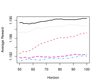
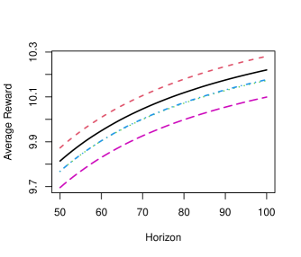
Figure 1: The average rewards of five policies over horizons ranging from $50$ to $100$ when the initial state distribution is bivariate standard normal distribution (left) and the initial state distribution is $t$-distribution with degree of freedom $2$ (right). The black solid curve corresponds to the proposed robust policy using $c=0.5$, red short-dashed curve using $c=0.3$ and green dotted curve using $c=0.1$. The blue dashed curve with dots corresponds to the policy using the long-term average reward and purple long-dashed curve corresponds to the policy using the average cumulative discounted rewards with discount rate $\gamma=0.9$.

7 Discussion

In this work, we propose a robust criterion to evaluate a policy by average rewards with respect to a set of distributions centered at the policy induced stationary distribution. It can be shown to contain average rewards across varying planning horizons with different reference distributions. Based on this criterion, we developed a data-efficient learning method to estimate the corresponding optimal policy that can maximize the worst case performance of some uncertainty set, improving the generalizability of the learned policy. A rate-optimal regret bound, up to a logarithm factor, was established in terms of the number of trajectories and decision points in each trajectory. A numerical study demonstrates the decent performance of our proposed method.

In the following, we discuss the setting where the reward $R_{t}$ also depends on the current action. Define the expected reawrd by $r(s,a)=\mathbb{E}[R_{t}|S_{t}=s,A_{t}=a]$. If we consider $\Pi$ as a class of deterministic policies, then we can correspondingly define $\mathcal{U}^{\pi}_{c}$ as $\left\{\mathbb{E}^{\pi}_{u}\left[r(S,A)\right]\,|\,u\in\Lambda^{\pi}_{c}\right\}.$ To obtain $\pi^{\ast}_{c}$ using the modified $\mathcal{U}^{\pi}_{c}$, under the assumption that the essential minimums of $r(s,a)$ under $d^{\pi}$ are the same for every $\pi\in\Pi$, one can show that it is equivalent to solving $\max_{\pi\in\Pi,\beta\in\mathbb{R}}\left\{\beta-\frac{1}{\left(1-c\right)}\mathbb{E}^{\pi}_{d^{\pi}}\left[\left(-r(S,A)+\beta\right)_{+}\right]\right\}.$ If we consider a stochastic policy class, then we need to solve $\max_{\pi\in\Pi,\beta\in\mathbb{R}}\left\{\beta-\frac{1}{\left(1-c\right)}\mathbb{E}_{d^{\pi}}\left[\left(-\sum_{a\in\mathcal{A}}\pi(a\,|\,S)r(S,a)+\beta\right)_{+}\right]\right\}.$ To obtain estimators for the above two objective functions, we need to implement an additional step by estimating the conditional reward function $r(s,a)$. This can be done by using some standard supervised learning techniques. In some applications, it may be more natural to define the reward as a function of the next state. In this case, one can include the reward into the state and still use our reward formulation.

Lastly, we discuss some future research directions. From the theoretical perspective, it will be interesting to derive the finite sample regret bound for the batch policy learning in the infinite-horizon MDP without stationarity and positivity assumptions. From the optimization perspective, our current algorithm requires a moderate computation and large memory due to the nonparametric estimation and the policy-dependent structure of nuisance functions. It is thus desirable to develop a more computationally efficient algorithm. One possible remedy is to consider zero-order optimization method. In the proposed algorithm, we consider tuning parameters independent of the policy. It will be interesting to investigate a more general setting and study how to perform model selection in batch RL, which seems far less studied in the literature. Another possible line of the research is to extend our proposed efficient policy learning method from the batch setting to the online setting. One challenging question is how to design an online algorithm to balance the evaluation of a policy and the search for a new policy given that all nuisance functions are policy dependent. Studying two-timescale stochastic algorithms such as Konda et al. (2004) may be a good starting point.

Appendix A Introduction

In Section 2 of this Supplementary Material, we provide details about computing $\widehat{\pi}^{c}_{N}$, and show how to select all tuning parameters in our learning method and also the constant $c$ in determining the size of $\Lambda_{c}^{\pi}$. In Section 3, we give all our technical proofs of theoretical results in the main text.

Appendix B Optimization and related computation

We start with our overall optimization problem.

Upper level optimization task:

$$\max_{\pi\in\Pi,\beta\in\mathbb{R}} \frac{\mathbb{P}_{n}\left\{(1/T_{0})\sum_{t=1}^{T_{0}}\widehat{\omega}^{\pi}_{N}(S_{t},A_{t})\left[\beta-\frac{1}{1-c}\left(\beta-R_{t}\right)_{+}+\widehat{U}^{\pi,\beta}_{N}(S_{t},A_{t},S_{t+1})\right]\right\}}{\mathbb{P}_{n}\left\{(1/T_{0})\sum_{t=1}^{T_{0}}\widehat{\omega}^{\pi}_{N}(S_{t},A_{t})\right\}}$$ (38)

Lower level optimization task 1:

$$(\widehat{\eta}_{N}^{\pi,\beta},\widehat{Q}_{N}^{\pi,\beta})=\operatorname*{argmin}_{(\eta,Q)\in\mathbb{R}\times\mathcal{F}_{1}}\mathbb{P}_{n}\left[\frac{1}{T_{0}}\sum_{t=1}^{T_{0}}\left[\widehat{g}_{N}^{\pi,\beta}(S_{t},A_{t};\eta,Q)\right]^{2}\right]+\lambda_{1N}J_{1}^{2}(Q)$$ (39)

$$\text{such that}\;\;\widehat{g}_{N}^{\pi,\beta}(\cdot,\cdot;\eta,Q)=\operatorname{argmin}_{h\in\mathcal{G}_{1}}\mathbb{P}_{n}\Big{[}\frac{1}{T_{0}}\sum_{t=1}^{T_{0}}\big{(}\delta^{\pi,\beta}(Z_{t};\eta,Q)-g(S_{t},A_{t})\big{)}^{2}\Big{]}+\mu_{1N}J_{2}^{2}(g)$$ (40)

Lower level optimization task 2:

$$\widehat{H}_{N}^{\pi}(\cdot,\cdot)=\operatorname*{argmin}_{H\in\mathcal{F}_{2}}\mathbb{P}_{n}\Big{[}\frac{1}{T_{0}}\sum_{t=1}^{T_{0}}\widehat{h}^{2}_{N}(S_{t},A_{t};H)\Big{]}+\lambda_{2N}J_{1}^{2}(H)$$ (41)

$$\text{such that}\,\,\widehat{h}_{N}(\cdot,\cdot;H)=\operatorname*{argmin}_{h\in\mathcal{G}_{2}}\mathbb{P}_{n}\Big{[}\frac{1}{T_{0}}\sum_{t=1}^{T_{0}}\big{(}\Delta^{\pi}(Z_{t};H)-h(S_{t},A_{t})\big{)}^{2}\Big{]}+\mu_{2N}J_{2}^{2}(h),$$ (42)

where we recall that $\delta^{\pi,\beta}(Z_{t};\eta,Q)=\beta-\frac{1}{1-c}\left(\beta-R_{t}\right)_{+}+\sum_{a^{\prime}}\pi(a^{\prime}|S_{t+1})Q(S_{t+1},a)-Q(S_{t},A_{t})-\eta$, $\widehat{U}^{\pi,\beta}_{N}(s,a,s^{\prime})=\sum_{a\in\cal A}\pi(a|s^{\prime})\widehat{Q}^{\pi,\beta}_{N}(s^{\prime},a)-\widehat{Q}^{\pi,\beta}_{N}(s,a)$, $\Delta^{\pi}(Z_{t};H)=1-H(S_{t},A_{t})+\sum_{a^{\prime}}\pi(a^{\prime}|S_{t+1})H(S_{t+1},a^{\prime})$, and $\widehat{\omega}^{\pi}_{N}(s,a)=\widehat{h}_{N}(s,a;\widehat{H}_{N}^{\pi})/\mathbb{P}_{n}[(1/T)\sum_{t=1}^{T}\widehat{h}_{N}(s,a;\widehat{H}_{N}^{\pi})]$.

B.1 Optimization Algorithm

As discussed at the end of Section 4 of the main text, the overall optimization problem is bi-level, where the upper level serves for searching an optimal robust policy and the lower level represents feasible sets, i.e., the estimation of our nuisance functions. In order to compute (38), we first need to specify spaces i.e., $\mathcal{F}_{1},\mathcal{F}_{2},\mathcal{G}_{1}$ and $\mathcal{G}_{2}$. For simplicity, we assume $\mathcal{F}_{1}=\mathcal{F}_{2}$ and $\mathcal{G}_{1}=\mathcal{G}_{2}$ and consider all these spaces as reproducing kernel Hilbert spaces (RKHSs) with radial basis function. This kernel has the universal property that can approximate any continuous functions under some mild conditions. In addition, considering RKHSs promotes efficient computations due to the representer theorem. Note that two parallel lower level problems (39)-(40) and (41)-(42) can be regarded as two nested kernel ridge regressions. By using the representer theorem, we can compute closed-form solutions for all our nuisance functions. Next, we specify the policy class, where we consider a class of stochastic paramterized policies indexed by $\theta$. For example, if we consider the binary-action space, i.e., $\mathcal{A}=\{0,1\}$, then we can model $\Pi$ as

$$\Pi=\left\{\pi\;\middle|\;\pi(1\,|\,s,\theta)=\frac{\exp(s^{T}\theta)}{1+\exp(s^{T}\theta)},\;\;\|\theta\|_{\infty}\leq\bar{c},\;\;\theta\in\mathbb{R}^{d},\;\;s\in\mathcal{S}\right\},$$

where $\|\bullet\|_{\infty}$ is the infinity norm, $\bar{c}$ is some positive constant for keeping stochasticity of the learned policy. We remark that multiple action cases and other models for the policy class can be defined similarly.

For the remaining of this section, we describe our optimization algorithm to obtained our estimated policy $\widehat{\pi}_{N}^{c}$ and the estimated auxiliary parameter $\widehat{\beta}$. We propose to use the block update algorithm. For each iteration, we first fixed $\pi$ (or equivalently $\theta$), and maximize $\widehat{M}_{N}(\beta,\pi)$ over $\beta$. Note that this is an one-dimensional optimization problem, which thus can be solved efficiently with the guarantee of finding a minimum. We remark that $\widehat{M}_{N}(\beta,\pi)$ is a piecewise linear function with respect to $\beta$ and thus an optimal solution must be one element in the vector $\{R_{t}^{i}\}_{1\leq i\leq n,1\leq t\leq T_{0}}$. Next, we fixed $\beta$ and maximize $\widehat{M}_{N}(\beta,\pi)$ over $\pi$. We use a limited-memory Broyden-Fletcher-Goldfarb-Shanno algorithm with box constraints (L-BFGS-B) to compute the solution $\widehat{\theta}$ [Liu and Nocedal, 1989]. To avoid bad solutions, in this step, we randomly select multiple initial points and search for the best solution. The full procedure can be found in Algorithm 1.

1 Input: Data $\mathcal{D}_{n}$, initial $\theta_{0}$ and $\beta_{0}$, a constant $\bar{c}$, and tolerance $\epsilon_{tol}>0$.

2Repeat for $t=0,\cdots,$ do till $\left\|\theta_{t+1}-\theta_{t}\right\|\leq\min\left\{\left\|\theta_{t}\right\|_{2},1\right\}\epsilon_{tol}$

3Compute $\beta_{t+1}$ by maximizing $\widehat{M}_{N}(\beta,\pi_{\theta_{t}})$ over $\beta$ with an initial $\beta_{t}$;

4Compute $\theta_{t+1}$ by maximizing $\widehat{M}_{N}(\beta_{t+1},\pi)$ over $\Pi$ with an initial $\theta_{t}$.

Output: $\widehat{\theta}$ and $\widehat{\beta}$.

Algorithm 1 Maximize $\widehat{M}_{N}(\beta,\pi)$

Discussion of Step 4 in Algorithm 1: It is noted that Step 4 in Algorithm 1 only involves optimization over $\theta$ while keeping $\beta$ fixed. We rewrite the training data $\mathcal{D}_{n}$ into tuples $Z_{h}=\{S_{h},A_{h},R_{h},S_{h+1}\}$ for $h=1,\dots,N$, where $h$ indexes the tuple of transition sample in the training set $\mathcal{D}_{n}$, $S_{h}$ and $S_{h+1}$ are the current and next states and $R_{h}$ is the associated reward. Let $W_{h}=(S_{h},A_{h})$ be one state-action pair, and $W_{h}^{\prime}=(S_{h},A_{h},S_{h+1})$ be one state-action-next-state pair. Denote the kernel function for the state as $k_{0}(s_{1},s_{2})$, where $s_{1},s_{2}\in\mathcal{S}$. Then the state-action kernel function can be define as $k((s_{1},a_{1}),(s_{2},a_{2}))=\mathds{1}_{\{a_{1}=a_{2}\}}k_{0}(s_{1},s_{2})$. Recall that we have to restrict the function space $\mathcal{F}_{1}$ such that $Q(s^{*},a^{*})=0$ for all $Q\in\mathcal{F}_{1}$ and $\mathcal{F}_{2}$ such that $H(s^{*},a^{*})=0$ for all $H\in\mathcal{F}_{2}$ respectively so as to avoid the identification issue. For ease of presentation, in the following, we omit the subscript for $\mathcal{F}_{j}$ and $\mathcal{G}_{j}$ when there is no confusion. Thus for any given kernel function $k$ defined on $\mathcal{S}\times\mathcal{A}$, we make the following transformation by defining $k(W_{1},W_{2})=k(W_{1},W_{2})-k((s^{*},a^{*}),W_{2})-k(W_{1},(s^{*},a^{*}))+k((s^{*},a^{*}),(s^{*},a^{*}))$ with some abuse of notations. One can check that the induced RKHS by this $k(\cdot,\cdot)$ satisfies the constraint in $\mathcal{F}$ automatically.

We denote kernel functions for $\mathcal{F}$ and $\mathcal{G}$ by $k(\cdot,\cdot),l(\cdot,\cdot)$ respectively. The corresponding inner products are defined as $\langle\cdot,\cdot\rangle_{\mathcal{F}}$ and $\langle\cdot,\cdot\rangle_{\mathcal{G}}$. In terms of the inner minimization problem (39)-(40), the closed form solution can be obtained by representer theorem. For example, $\widehat{g}^{\pi,\beta}_{N}(\cdot,\cdot;\eta,Q)=\sum_{h=1}^{N}l(W_{h},\cdot)\widehat{\gamma}(\eta,Q)$, where $\widehat{\gamma}(\eta,Q)=(L+\mu_{1}I_{N})^{-1}\delta_{N}^{{\pi}}(\eta,Q)$, $L$ is the kernel matrix of $l$, $\mu_{1}=\mu_{1N}N$, and $\delta^{\pi}_{N}(\eta,Q)=(\delta^{\pi}(W^{\prime}_{h};\eta,Q))_{h=1}^{N}$ is a vector of TD error. Moreover, each temporal difference error can be further written as $\delta^{\pi,\beta}(W^{\prime}_{h};\eta,Q)=\beta-\frac{1}{1-c}\left(\beta-R\right)_{+}-\eta-\langle Q,\tilde{k}_{W^{\prime}}\rangle_{\mathcal{G}}$, where

$$\tilde{k}_{W^{\prime}}(\cdot)=k(W,\cdot)-\sum_{a^{\prime}}\pi(a^{\prime}|S^{\prime})k((S^{\prime},a^{\prime}),\cdot)\in\mathcal{F}$$

One can demonstrate that $\widehat{Q}^{\pi,\beta}_{N}$ in (39) can be expressed by the linear span: $\{\sum_{h=1}^{N}\alpha_{h}\tilde{k}_{W_{h}^{\prime}}(\cdot):\alpha_{h}\in\mathbb{R},h=1,\dots,N\}$ according to the representer property. Then the optimization problem (39)-(40) is equivalent to solving

$$(\widehat{\eta}_{N}^{\pi,\beta},\widehat{\alpha}(\pi,\beta))=\operatorname*{argmin}_{\eta\in\mathbb{R},\alpha\in\mathbb{R}^{N}}(R^{\beta}_{N}-\eta 1_{N}-\tilde{K}(\pi)\alpha)^{\top}M(R^{\beta}_{N}-\eta 1_{N}-\tilde{K}(\pi)\alpha)+\lambda_{1}\alpha^{\top}\tilde{K}(\pi)\alpha$$ (43)

where $R^{\beta}_{N}=(\beta-\frac{1}{1-c}\left(\beta-R_{h}\right)_{+})_{h=1}^{N}$, $\tilde{K}(\pi)=(\langle\tilde{k}_{W_{h}^{\prime}},\tilde{k}_{W_{j}^{\prime}}\rangle_{\mathcal{F}})_{j,h=1}^{N}$, $M=(L+\mu_{1}I_{N})^{-1}L^{2}(L+\mu_{1}I_{N})^{-1}$, $1_{N}$ is a length-$N$ vector of all ones, $\lambda_{1}=\lambda_{1N}N$ and $\alpha=(\alpha_{h})_{h=1}^{N}$ is a vector of length $N$. Note that the $(h,k)$-th element of the matrix $\tilde{K}(\pi)\left[h,k\right]$ can be further calculated as

$$\langle\tilde{k}_{W_{h}^{\prime}},\tilde{k}_{W_{j}^{\prime}}\rangle_{\mathcal{F}} =k(W_{h},W_{j})-\sum_{a^{\prime}}\pi(a^{\prime}|S_{h}^{\prime})k((S_{h}^{\prime},a^{\prime}),W_{j})-\sum_{a^{\prime}}\pi(a^{\prime}|S_{j}^{\prime})k((S_{j}^{\prime},a^{\prime}),W_{h})$$

$$\qquad+\sum_{a_{h}^{\prime}}\sum_{a_{j}^{\prime}}\pi(a_{h}^{\prime}|S_{h}^{\prime})\pi(a_{j}^{\prime}|S_{j}^{\prime})k((S_{h}^{\prime},a_{h}^{\prime}),(S_{j}^{\prime},a_{j}^{\prime})).$$

We make $\tilde{K}(\pi)$ and $\widehat{\alpha}(\pi,\beta)$ as functions of $\pi$ and $\beta$ to explicitly indicate their dependency on the policy $\pi$ and the auxiliary parameter $\beta$. The first-order optimality implies that $(\widehat{\eta}_{N}^{\pi,\beta},\widehat{\alpha}(\pi,\beta))$ satisfies

$$1_{N}^{\top}M1_{N}\widehat{\eta}_{N}^{\pi,\beta}=1_{N}^{\top}M(R^{\beta}_{N}-\tilde{K}(\pi)\widehat{\alpha}(\pi,\beta))$$

$$(M\tilde{K}(\pi)+\lambda_{1}I_{N})\widehat{\alpha}(\pi,\beta)=M(R^{\beta}_{N}-M1_{N}\widehat{\eta}_{N}^{\pi,\beta}),$$

which gives

$$(M\tilde{K}(\pi)+\lambda_{1}I_{N}-MF(1_{N}^{T}M1_{N})^{-1}1_{N}^{T}M\tilde{K}(\pi))\widehat{\alpha}(\pi,\beta)$$ (44)

$$= (I_{N}-1_{N}(1_{N}^{T}M1_{N})^{-1}1_{N}^{T})MR^{\beta}_{N}$$ (45)

and thus the corresponding $\{\widehat{U}_{N}^{\pi}(W^{\prime}_{h})\}_{h=1}^{N}=-\tilde{K}(\pi)\widehat{\alpha}(\pi,\beta)$. In order to apply L-BFGS-B, we need to compute the Jacobian matrix of the vector $\{\widehat{U}_{N}^{\pi}(W^{\prime}_{h})\}_{h=1}^{N}$ with respect to $\theta$. Based on the above equations, we know

$$\frac{\partial\{\widehat{U}_{N}^{\pi}(W^{\prime}_{h})\}_{h=1}^{N}}{\partial\theta}=-\frac{\partial\tilde{K}(\pi)}{\partial\theta}\otimes\widehat{\alpha}(\pi,\beta)-\tilde{K}(\pi)\frac{\partial\widehat{\alpha}(\pi,\beta)}{\partial\theta},$$

where $\otimes$ is denoted as a tensor product. Here $\frac{\partial\tilde{K}(\pi)}{\partial\theta}$ is a $\mathbb{R}^{N}\otimes\mathbb{R}^{N}\otimes\mathbb{R}^{p}$ tensor, where the $(i,j,k)$-th element is the partial derivative $\frac{\partial\left[\tilde{K}(\pi)\right]_{i,j}}{\partial\theta_{k}}$. In addition, $\frac{\partial\widehat{\alpha}(\pi,\beta)}{\partial\theta}$ can be calculated via implicit theorem based on the equation (44)-(45), i.e.,

$$\left(M\otimes\frac{\partial\tilde{K}(\pi)}{\partial\theta}+\lambda I_{N}-MF(1_{N}^{T}M1_{N})^{-1}1_{N}^{T}M\otimes\frac{\partial\tilde{K}(\pi)}{\partial\theta}\right)\widehat{\alpha}(\pi,\beta)$$ (46)

$$= -(M\tilde{K}(\pi)+\lambda I_{N}-MF(1_{N}^{T}M1_{N})^{-1}1_{N}^{T}M\tilde{K}(\pi))\frac{\partial\widehat{\alpha}(\pi,\beta)}{\partial\theta},$$ (47)

which gives the expression of $\frac{\partial\widehat{\alpha}(\pi)}{\partial\theta}$, a $N$ by $p$ matrix.

We can use the same approach to get the closed-form solution for the problem (41)-(42) and compute its corresponding gradient with respect to $\theta$. By some calculation, we can get $\{\widehat{h}_{N}^{\pi}(W_{j},\widehat{H}^{\pi}_{N})\}_{j=1}^{N}=L\widehat{\nu}(\pi)$, where $\widehat{h}_{N}^{\pi}(W_{j},\widehat{H}^{\pi}_{N})=\sum_{j=1}^{N}\widehat{\nu}_{j}(\pi)l(W_{j},\cdot)$ and $\nu=(\widehat{\nu}_{j}(\pi))_{j=1}^{N}$ satisfying the following two equations:

$$(M\tilde{K}(\pi)+\lambda_{2}I_{N})\widehat{\varphi}(\pi) =M1_{N}$$ (48)

$$(L+\mu_{2}I_{N})\widehat{\nu}(\pi) =1_{N}-\tilde{K}(\pi)\widehat{\varphi}(\pi),$$ (49)

again by the representer theorem, where $\widehat{\varphi}(\pi)$ is estimated coefficient associated with $\tilde{K}(\pi)$, $\lambda_{2}=\lambda_{2N}N$ and $\mu_{2}=\mu_{2N}N$. The Jacobian matrix of $\{\widehat{h}_{N}^{\pi}(W_{j},\widehat{H}^{\pi}_{N})\}_{j=1}^{N}$ can be computed by again using the implicit theorem on equations (48) and (49). More specifically, we need to solve $\frac{\partial\widehat{\nu}(\pi)}{\partial\theta}$ based on the following two equations.

$$\left(M\otimes\frac{\partial\tilde{K}(\pi)}{\partial\theta}\right)\widehat{\varphi}(\pi)+\left(M\tilde{K}(\pi)+\lambda_{2}I_{N}\right)\frac{\partial\widehat{\varphi}(\pi)}{\partial\theta} =0.$$ (50)

$$(L+\mu_{2}I_{N})\frac{\partial\widehat{\nu}(\pi)}{\partial\theta}+\tilde{K}(\pi)\frac{\partial\widehat{\varphi}(\pi)}{\partial\theta}+\frac{\partial\tilde{K}(\pi)}{\partial\theta}\otimes\frac{\partial\widehat{\varphi}(\pi)}{\partial\theta} =0.$$ (51)

Then we have

$$\frac{\partial\{\widehat{g}_{N}^{\pi,\beta}(W_{h},\widehat{H}^{\pi}_{N})\}_{j=1}^{N}}{\partial\theta}=L\frac{\partial\widehat{\nu}(\pi)}{\partial\theta}.$$

Summarizing together by plugging all the intermediate results into the objective function of our upper optimization problem (38), we can simplify step 4 in Algorithm 1 as

$$\max_{\pi\in\Pi_{\Theta}} \frac{\left(\widehat{\nu}(\pi)\right)^{T}L\left(R^{\beta}_{N}-\tilde{K}(\pi)\widehat{\alpha}(\pi,\beta)\right)}{\widehat{\nu}(\pi)^{T}L1_{N}}.$$ (52)

The corresponding gradient with respect to $\theta$ can be computed directly as

$$\frac{\left(\frac{\partial\widehat{\nu}(\pi)}{\partial\theta}\right)^{T}L\left(R^{\beta}_{N}-\tilde{K}(\pi)\widehat{\alpha}(\pi,\beta)\right)-\left(\widehat{\nu}(\pi)\right)^{T}L\left(\frac{\partial\tilde{K}(\pi)}{\partial\theta}\otimes\widehat{\alpha}(\pi,\beta)+\tilde{K}(\pi)\frac{\partial\widehat{\alpha}(\pi,\beta)}{\partial\theta}\right)\left(\widehat{\nu}(\pi)^{T}L1_{N}\right)}{\left(\widehat{\nu}(\pi)^{T}L1_{N}\right)^{2}}$$

$$- \frac{\left(\frac{\partial\widehat{\nu}(\pi)}{\partial\theta}\right)^{T}L\left(R^{\beta}_{N}-\tilde{K}(\pi)\widehat{\alpha}(\pi,\beta)\right)\left(\widehat{\nu}(\pi)^{T}L1_{N}\right)}{\left(\widehat{\nu}(\pi)^{T}L1_{N}\right)^{2}}.$$

B.2 Selection of Tuning Parameters

In this subsection, we discuss the choice of tuning parameters in our method. The bandwidths in the Gaussian kernels are selected using median heuristic, e.g., median of pairwise distance [Fukumizu et al., 2009]. The tuning parameters $(\lambda_{1N},\mu_{1N})$ and $(\lambda_{2N},\mu_{2N})$ are selected based on 3-fold cross-validation. We assume that all these tuning parameters are independent of the policy $\pi$ and $\beta$ so that we can select them based the estimation of ratio and relative value functions using some randomly generated policies and $\beta$. We adopt ideas from [Farahmand and Szepesvári, 2011] and [Liao et al., 2020]. Specifically, for the tuning parameters $(\lambda_{1N},\mu_{1N})$ in the estimation of relative value function, we focus on (39)-(40) using cross-validation. For the tuning parameters $(\lambda_{2N},\mu_{2N})$ in the estimation of ratio function, we focus on (41)-(42). Both of the cross-validation procedures are based on choosing the tuning parameters that have the smallest estimated projected bellman errors on the validation set among a pre-specified tuning set. The details of selecting these tuning parameters can be found in Algorithm 2.

1 Input: Data $\{Z_{h}\}_{h=1}^{N}$, a set of $M$ policies $\left\{\pi_{1},\cdots,\pi_{M}\right\}\subset\Pi$, a set of $\left\{\beta_{1},\cdots,\beta_{L}\right\}$, a set of $J$ candidate tuning parameters $\{(\mu^{(j)}_{1N},\lambda^{(j)}_{1N})\}_{j=1}^{J}$ in the relative value function estimation, and a set of $J$ candidate tuning parameters $\{(\mu^{(j)}_{2N},\lambda^{(j)}_{2N})\}_{j=1}^{J}$ in the ratio function estimation.

2Randomly split Data into $K$ subsets: $\{Z_{h}\}_{h=1}^{N}=\left\{D_{k}\right\}_{k=1}^{K}$

3Denote $e^{(1)}(m,l,j)$ and $e^{(2)}(m,l,j)$ as the total validation error for $m$-th policy, $l$-th $\beta$ and $j$-th pair of tuning parameters in value and ratio function estimation respectively, for $m=1,\cdots M$, $l=1,\cdots,L$ and $j=1,\cdots,J$. Set their initial values as $0$.

4Repeat for $m=1,\cdots,M$,

5Repeat for $l=1,\cdots,L$,

6Repeat for $k=1,\cdots,K$,

7Repeat for $j=1,\cdots,J$

8Use $\{Z_{h}\}_{h=1}^{N}\backslash D_{k}$ to compute $(\widehat{\eta}_{N}^{\pi_{m},\beta_{l}},\widehat{\alpha}(\pi_{m},\beta))$ and $\widehat{\nu}(\pi_{m},\beta_{l})$ by (39)-(40) and (41)-(42) using tuning parameters $(\mu^{(j)}_{1N},\lambda^{(j)}_{1N})$ and $(\mu^{(j)}_{2N},\lambda^{(j)}_{2N})$ respectively;

9Compute $\delta^{\pi_{m},\beta_{l}}(\cdot;\widehat{\eta}^{\pi_{m},\beta_{l}},\widehat{Q}_{N}^{\pi_{m},\beta_{l}})$ and $\Delta^{\pi_{m}}(\cdot;\widehat{H}_{N}^{\pi_{m}})$ and their corresponding squared Bellman errors $mse^{(1)}$ and $mse^{(2)}$ on the dataset $D_{k}$ by Gaussian kernel regression;

10Assign $e^{(1)}(m,l,j)=e^{(1)}(m,l,j)+mse^{(1)}$ and $e^{(2)}(m,j)=e^{(2)}(m,j)+mse^{(2)}$;

11

12Compute $j^{(1)\ast}\in\operatorname{argmin}_{j}\max_{m,l}e^{(1)}(m,l,j)$ and $j^{(2)\ast}\in\operatorname{argmin}_{j}\max_{m}e^{(2)}(m,j)$

Output: $(\mu_{1N}^{j^{(1)\ast}},\lambda_{1N}^{j^{(1)\ast}})$ and $(\mu_{2N}^{j^{(2)\ast}},\lambda_{2N}^{j^{(2)\ast}})$.

Algorithm 2 Tuning parameters selection via cross-validation

B.3 Selection of Constant $c$ in $\Lambda^{\pi}_{c}$

It is important to choose a proper constant $c$ in $\Lambda^{\pi}_{c}$ in order to protect against uncertainty in terms of the duration of use of the policy in future and different reference distributions. If we choose $c=1$, (2) in the main text becomes $R_{\min}$ for all $\pi\in\Pi$ and thus we are unable to distinct different policies because we are over conservative. If $c=0$, (2) in the main text becomes the long-term average reward, where we basically ignore any rewards happened in any finite period of time. If we know at least how long the learned policy will be implemented in the future, say $T_{0}$, and how fast the policy-induced Markov chain converges to the stationary distribution, we can choose $c$ properly. For example, we have the following uniform ergodic theorem given in Theorem 7.3.10 of Hernández-Lerma and Lasserre [2012].

Theorem B.1 (Uniform Geometric Ergodicity)

If for any $\pi\in\Pi$, the induced Markov chain $P^{\pi}$ is $\psi$-irreducible and aperiodic and satisfies the geometric drift condition described in Theorem 7.3.1 of [Hernández-Lerma and Lasserre, 2012], then there exist constants $0<\alpha(\pi)<1$ and $C_{0}(\pi)>0$ such that,

$$\max_{s\in\mathcal{S}}\left\|P^{\pi}_{t}(\bullet\,|\,S_{1}=s)-d^{\pi}(\bullet)\right\|_{\text{TV}}\leq\min\left(1,C_{0}(\pi)\alpha^{t}(\pi)\right).$$

Indeed, this theorem can further imply that for any $\tilde{\mathbb{G}}\in\Lambda$

$$\left\|\bar{d}^{\pi}_{T;\tilde{\mathbb{G}}}(\bullet)-d^{\pi}(\bullet)\right\|_{\text{TV}}\leq\min\left(1,\frac{C_{0}(\pi)\alpha(\pi)}{1-\alpha(\pi)}\frac{1}{T}\right).$$

As we can see, the average visiting distribution of the induced Markov chain converges sublinearly to the unique stationary distribution in terms of time $T$. If we assume there exists some positive constants $\tilde{\alpha}<1$ and $\tilde{C}_{0}$ independent of $\pi$ that the above inequality holds uniformly over $\Pi$, then we can choose $c$ based on these constants. For example, if we know $\tilde{\alpha}\leq 0.9$, $\tilde{C}_{0}\leq 1$, and $T_{0}=100$, then we can choose $c=\frac{0.9}{100(1-0.9)}=0.09$, so that $\mathcal{U}^{\pi}_{T_{0}}\subseteq\mathcal{U}_{c}^{\pi}$, which satisfies our need. In practice, one also needs to consider the estimation error in terms of $c$. As we can see from (4) in the main text, if we choose $c$ large, the set $\Lambda_{c}^{\pi}$ is large, thus requiring more data to estimate $\pi^{\ast}_{c}$ than that of smaller $c$ in order to achieve the same level of the accuracy. In contrast, a larger $c$ can guarantee a more robust policy than a smaller $c$ because we consider more uncertain scenarios. The remaining question is how to estimate $\tilde{\alpha}$ and $\tilde{C}_{0}$ using $D_{n}$, which we leave it as a future work.

Appendix C Technical Proofs

In this section, we provide all the technical proofs to the theoretical results in the main text. The notation $K(N)\lesssim L(N)$ (resp. $K(N)\gtrsim L(N)$) means that there exist a sufficiently large constant (resp. small) constant $c_{1}>0$ (resp. $c_{2}>0$) such that $K(N)\geq c_{1}L(N)$ (resp. $K(N)\leq c_{2}L(N)$). Moreover, $K(N)\simeq L(N)$ means $K(N)\lesssim L(N)$ and $K(N)\gtrsim L(N)$. All these constants do not depend on data, i.e., deterministic. For notational simplicity, we omit $\beta$, the auxiliary variable in the relative value function $Q^{\pi,\beta}$, its difference $U^{\pi,\beta}$, temporal difference $\delta^{\pi,\beta}$ and their related estimators when there is no confusion. Finally, we also denote $T=T_{0}$, $\mu_{jN}=\mu_{N}$, $\lambda_{jN}=\lambda_{N}$, $\mathcal{F}_{j}=\mathcal{F}$ and $\mathcal{G}_{j}=\mathcal{G}$ for the ease of presentation when there is no confusion.

Definition C.1 (Covering Number)

Let $\epsilon>0$, $\mathcal{F}$ be a set of real-valued functions defined over some space $\mathcal{X}$. For a finite collection of $N_{\epsilon}=\{f_{1},\cdots,f_{N_{\epsilon}}\}$ defined on $\mathcal{X}$ such that for every $f\in\mathcal{F}$, there exits a function $\bar{f}\in N_{\epsilon}$ that $\text{dist}(f-\bar{f})\leq\epsilon$ is called an $\epsilon$-cover of $\mathcal{F}$ with respect to the metric $\text{dist}({\bullet})$. Let $\mathcal{N}(\epsilon,\mathcal{F},\text{dist}({\bullet}))$ be the size of the smallest $\epsilon$-cover of $\mathcal{F}$ with respect to $\text{dist}({\bullet})$.

C.1 Proof of Theorem 4.1

It can be seen that the defined function $\phi(x)$ is convex. By the results in [Shapiro, 2017] [section 3.2], we can show that

$$\max_{u\in\Lambda^{\pi}_{c}}\,\,-\mathbb{E}_{d^{\pi}}\left[\mathcal{R}(S)\right]=\min_{\lambda\geq 0,\beta}\lambda c+\beta+\mathbb{E}_{d^{\pi}}\left[\left(\lambda\phi\right)^{\ast}\left(-\mathcal{R}(S)-\beta\right)\right],$$

where the function $\left(\lambda\phi\right)^{\ast}(\bullet)$ refers to the conjugate of $\lambda\phi(\bullet)$. Note that we modify the left hand side above into a maximization problem to be consistent with results in [Shapiro, 2017]. Then by the definition of $\phi(x)$, we have that

$$\left(\lambda\phi\right)^{\ast}(x)=\begin{cases}-\frac{\lambda}{2}+\left(x+\frac{\lambda}{2}\right)_{+}&x\leq\frac{\lambda}{2}\\[7.22743pt] +\infty&x>\frac{\lambda}{2}\end{cases},$$

where $\left(\bullet\right)_{+}=\max(0,\bullet)$. Then we have the following equivalent formulation.

$$\min_{\lambda\geq 0,\beta}\lambda c+\beta+\mathbb{E}_{d^{\pi}}\left[\left(\lambda\phi\right)^{\ast}\left(-\mathcal{R}(S)-\beta\right)\right]$$

$$= \min_{\begin{subarray}{c}\beta,\lambda\geq 0,\\ \lambda\geq-(2R_{\min}+2\beta)\end{subarray}}\lambda c+\beta-\frac{\lambda}{2}+\mathbb{E}_{d^{\pi}}\left[\left(-\mathcal{R}(S)+\frac{\lambda}{2}-\beta\right)_{+}\right]$$

$$= \min_{\begin{subarray}{c}\beta,\lambda\geq 0,\\ \lambda\geq-(R_{\min}+\beta)\end{subarray}}\lambda c+\beta+\mathbb{E}_{d^{\pi}}\left[\left(-\mathcal{R}(S)-\beta\right)_{+}\right]$$

$$= \min_{\lambda\geq 0}\lambda c-R_{\min}-\lambda+\mathbb{E}_{d^{\pi}}\left[\left(-\mathcal{R}(S)+R_{\min}+\lambda\right)_{+}\right]$$

$$= -cR_{\min}+\min_{\beta\geq R_{\min}}-\left(1-c\right)\beta+\mathbb{E}_{d^{\pi}}\left[\left(-\mathcal{R}(S)+\beta\right)_{+}\right]$$

$$= -cR_{\min}-\left(1-c\right)\max_{\beta\in\mathcal{R}}\left\{\beta-\frac{1}{\left(1-c\right)}\mathbb{E}_{d^{\pi}}\left[\left(-\mathcal{R}(S)+\beta\right)_{+}\right]\right\},$$

where the first equality uses the definition of $\left(\lambda\phi\right)^{\ast}(x)$ and the assumption in this theorem, the second equality changes the variable $\beta\leftarrow(\beta-\frac{\lambda}{2})$, the third equality uses the monotonicity with respect with $\beta$, the fourth equality changes the variable $\beta\leftarrow(\lambda+R_{\min})$ and the last inequality is because the optimal solution is within the feasible set. Therefore, we have the first statement and the second statement follow immediately as below.

$$\operatorname{argmax}_{\pi\in\Pi}\min_{u\in\Lambda^{\pi}_{c}}\mathbb{E}_{d^{\pi}}\left[\mathcal{R}(S)\right]$$

$$= \operatorname{argmax}_{\pi\in\Pi}\max_{\beta\in\mathbb{R}}\left\{\beta-\frac{1}{\left(1-c\right)}\mathbb{E}_{d^{\pi}}\left[\left(-\mathcal{R}(S)+\beta\right)_{+}\right]\right\}.$$

C.2 Finite Sample Error Bound for the Relative Value Difference Function

Proof of Theorem 5.1 Denote $\bar{B}=[-R_{\max},R_{\max}]$. By Lemma C.2 given by Assumption 5.1, we have

$$\sup_{\pi\in\Pi,\beta\in\bar{B}}\|\widehat{U}^{\pi,\beta}_{N}-U^{\pi,\beta}\|\leq\left(1+\frac{1}{p_{\min}}\right)\sup_{\pi\in\Pi,\beta\in\bar{B}}\|\widehat{Q}_{N}^{\pi,\beta}-Q^{\pi,\beta}\|.$$

By the definition of $\widehat{U}^{\pi,\beta}$, we can assume that the expectation of $\widehat{Q}_{N}^{\pi,\beta}$ under the stationary distribution is 0, otherwise we can shift $\widehat{Q}_{N}^{\pi,\beta}$ by a constant to obtain it. Then we apply Lemma C.3 and Lemma C.4 below to get

$$\sup_{\pi\in\Pi,\beta\in\bar{B}}\|\widehat{U}^{\pi,\beta}_{N}-U^{\pi,\beta}\| \lesssim 2\left(1+\frac{1}{p_{\min}}\right)\sup_{\pi\in\Pi,\beta\in\bar{B}}\|(\,\mathcal{I}-\mathcal{P}^{\pi})\left(\widehat{Q}_{N}^{\pi,\beta}-Q^{\pi,\beta}\right)\|$$

$$\lesssim 2\left(1+\frac{1}{p_{\min}}\right)(1+\sqrt{1+\sup_{\pi\in\Pi}\sigma_{\pi}^{2}})\sup_{\pi\in\Pi,\beta\in\bar{B}}\|\mathcal{E}_{\pi}(\widehat{\eta}_{N}^{\pi,\beta},\widehat{Q}_{N}^{\pi,\beta})\|,$$

where $\sigma^{2}_{\pi}$ is the variance of $\omega^{\pi}$and $\mathcal{E}_{\pi,\beta}$ is the bellman error, i.e.,

$$\mathcal{E}_{\pi,\beta}(s,a;\eta,Q)\triangleq\mathbb{E}\left[\beta-\frac{1}{1-c}\left(\beta-R_{t}\right)_{+}+\sum_{a^{\prime}}\pi(a^{\prime}|S_{t+1})Q(S_{t+1},a^{\prime})-\eta-Q(s,a)\,|\,S_{t}=s,A_{t}=a\right].$$

Since $\|w^{\pi}\|^{2}=1+\sigma_{\pi}^{2}$ and by Assumption 5.1 (d), $\sup_{\pi\in\Pi}\sigma_{\pi}^{2}<\infty$.

Next, we derive the uniform error bound for $\sup_{\pi\in\Pi,\beta\in\bar{B}}\|\mathcal{E}_{\pi,\beta}(\widehat{\eta}_{N}^{\pi,\beta},\widehat{Q}_{N}^{\pi,\beta})\|$. Let

$$\mathcal{T}_{\pi}(s,a;Q)=\mathbb{E}\left[\beta-\frac{1}{1-c}\left(\beta-R_{t}\right)_{+}+\sum_{a^{\prime}}\pi(a^{\prime}|S_{t+1})Q(S_{t+1},a^{\prime})\,|\,S_{t}=s,A_{t}=a\right].$$

By the definition of $\kappa$ in Assumption 5.2(c),

$$\sup_{\pi\in\Pi,\beta\in\bar{B}}\|\mathcal{E}_{\pi,\beta}(\widehat{\eta}_{N}^{\pi,\beta},\widehat{Q}_{N}^{\pi,\beta})\|^{2}=\sup_{\pi\in\Pi,\beta\in\bar{B}}\|\mathcal{T}_{\pi}(\cdot,\cdot;\widehat{Q}_{N}^{\pi,\beta})-\widehat{\eta}^{\pi,\beta}_{N}-\widehat{Q}_{N}^{\pi,\beta}(\cdot,\cdot)\|^{2}$$

$$\leq\frac{1}{\kappa^{2}}\sup_{\pi\in\Pi,\beta\in\bar{B}}\|g^{*}_{\pi}(\widehat{\eta}_{N}^{\pi,\beta},\widehat{Q}_{N}^{\pi,\beta})\|^{2}\leq\frac{2}{\kappa^{2}}\left(\sup_{\pi\in\Pi,\beta\in\bar{B}}\|g^{*}_{\pi}(\widehat{\eta}_{N}^{\pi,\beta},\widehat{Q}_{N}^{\pi,\beta})-\widehat{g}^{\pi,\beta}_{N}(\widehat{\eta}_{N}^{\pi,\beta},\widehat{Q}_{N}^{\pi,\beta})\|^{2}+\sup_{\pi\in\Pi,\beta\in\bar{B}}\|\widehat{g}^{\pi,\beta}_{N}(\widehat{\eta}_{N}^{\pi,\beta},\widehat{Q}_{N}^{\pi,\beta})\|^{2}\right).$$ (53)

We first consider the second term in the RHS of the above inequality. Using Lemma C.6 and letting $\tau\leq\frac{1}{3}$, with $N$ sufficiently large, the following holds with probability at least $1-\delta$:

$$\sup_{\pi\in\Pi,\beta\in\bar{B}}\|\widehat{g}_{N}^{\pi}(\widehat{\eta}_{N}^{\pi,\beta},\widehat{Q}_{N}^{\pi,\beta})\|^{2}$$

$$\lesssim\mu_{N}+\mu_{N}\sup_{\pi\in\Pi,\beta\in\bar{B}}J_{2}^{2}\left\{g^{\ast}_{\pi,\beta}(\eta^{\pi,\beta},\tilde{Q}^{\pi,\beta})\right\}+(\mu_{N}+\lambda_{N})\sup_{\pi\in\Pi,\beta\in\bar{B}}J_{1}^{2}(\tilde{Q}^{\pi,\beta})+\frac{(VC(\Pi)+1)\left[\log\left(\max(1/\delta,N)\right)\right]^{\frac{1}{\tau}}}{N}$$

$$+N^{-\frac{1-(2+\alpha)\tau}{1+\alpha-\tau(2+\alpha)}}+\frac{1+VC(\Pi)}{N\mu_{N}^{\alpha/(1-\tau(2+\alpha))}}+\frac{(VC(\Pi)+1)\log^{\frac{\alpha/\tau}{1+\alpha-\tau(2+\alpha)}}(\max(N,1/\delta))}{N\mu_{N}^{\alpha/(1+\alpha-(2+\alpha)\tau)}}+\frac{1}{N\lambda_{N}^{\frac{\alpha}{1-\tau(2+\alpha)}}}$$

$$\lesssim\mu_{N}\left(1+\sup_{\pi\in\Pi,\beta\in\bar{B}}J_{1}^{2}(\tilde{Q}^{\pi,\beta})\right)+\frac{(VC(\Pi)+1)\left[\log\left(\max(1/\delta,N)\right)\right]^{\frac{1}{\tau}}}{N}+N^{-\frac{1-(2+\alpha)\tau}{1+\alpha-\tau(2+\alpha)}}$$

$$+\frac{1+VC(\Pi)}{N\mu_{N}^{\alpha/(1-\tau(2+\alpha))}}+\frac{(VC(\Pi)+1)\log^{\frac{\alpha/\tau}{1+\alpha-\tau(2+\alpha)}}(\max(N,1/\delta))}{N\mu_{N}^{\alpha/(1+\alpha-(2+\alpha)\tau)}},$$

where we use the condition that $\lambda_{N}\simeq\mu_{N}$ and Assumption 5.2(d).

We now turn to the first term. By Lemma C.5 with the same $\tau$ used above and $N$ sufficiently large, we have at least probability $1-\delta$,

$$\sup_{\pi\in\Pi,\beta\in\bar{B}}\|\widehat{g}^{\pi}_{N}(\widehat{\eta}_{N}^{\pi,\beta},\widehat{Q}_{N}^{\pi,\beta})-g^{*}_{\pi}(\widehat{\eta}_{N}^{\pi},\widehat{Q}_{N}^{\pi})\|^{2} \lesssim\mu_{N}+\mu_{N}\sup_{\pi\in\Pi,\beta\in\bar{B}}J_{2}^{2}\left\{g^{*}_{\pi}(\widehat{\eta}_{N},\widehat{Q}_{N}^{\pi})\right\}+\mu_{N}\sup_{\pi\in\Pi,\beta\in\bar{B}}J_{1}^{2}(\widehat{Q}_{N}^{\pi})$$

$$+\frac{(VC(\Pi)+1)\left[\log\left(\max(1/\delta,N)\right)\right]^{\frac{1}{\tau}}}{N}+\frac{1+VC(\Pi)}{N\mu_{N}^{\frac{\alpha}{1-\tau(2+\alpha)}}}.$$

Using Assumption 5.2(d) again, this can be further bounded by

$$\sup_{\pi\in\Pi,\beta\in\bar{B}}\|\widehat{g}^{\pi,\beta}_{N}(\widehat{\eta}_{N}^{\pi,\beta},\widehat{Q}_{N}^{\pi,\beta})-g^{\ast}_{\pi,\beta}(\widehat{\eta}_{N}^{\pi,\beta},\widehat{Q}_{N}^{\pi,\beta})\|^{2} \lesssim\mu_{N}(1+\sup_{\pi\in\Pi,\beta\in\bar{B}}J_{2}^{2}(\widehat{Q}^{\pi,\beta}_{N}))+\frac{(VC(\Pi)+1)\left[\log\left(\max(1/\delta,N)\right)\right]^{\frac{1}{\tau}}}{N}$$

$$+\frac{1+VC(\Pi)}{N\mu_{N}^{\frac{\alpha}{1-\tau(2+\alpha)}}}$$ (54)

To bound $\sup_{\pi\in\Pi,\beta\in\bar{B}}J_{1}^{2}(\widehat{Q}_{N}^{\pi,\beta})$, the optimizing property of the estimators $(\widehat{\eta}_{N}^{\pi,\beta},\widehat{Q}_{N}^{\pi,\beta})$ in (39) implies that

$$\lambda_{N}J_{1}^{2}(\widehat{Q}_{N}^{\pi,\beta}) \leq\mathbb{P}_{n}\left[\frac{1}{T}\sum_{t=1}^{T}\widehat{g}^{\pi,\beta}_{N}(S_{t},A_{t};\widehat{\eta}_{N}^{\pi,\beta},\widehat{Q}_{N}^{\pi,\beta})^{2}\right]+\lambda_{N}J_{1}^{2}(\widehat{Q}_{N}^{\pi,\beta})$$

$$\leq\mathbb{P}_{n}\left[\frac{1}{T}\sum_{t=1}^{T}\widehat{g}^{\pi,\beta}_{N}(S_{t},A_{t};\eta^{\pi,\beta},\tilde{Q}^{\pi,\beta})^{2}\right]+\lambda_{N}J_{1}^{2}(\tilde{Q}^{\pi,\beta})$$

$$=\mathbb{P}_{n}\left[\frac{1}{T}\sum_{t=1}^{T}(\widehat{g}^{\pi,\beta}_{N}(S_{t},A_{t};\eta^{\pi,\beta},\tilde{Q}^{\pi,\beta})-g^{\ast}_{\pi,\beta}(S_{t},A_{t};\eta^{\pi,\beta},\tilde{Q}^{\pi,\beta}))^{2}\right]+\lambda_{N}J_{1}^{2}(\tilde{Q}^{\pi,\beta})$$

$$\lesssim\mu_{N}(1+J_{1}^{2}(\tilde{Q}^{\pi,\beta}))+\frac{(VC(\Pi)+1)\left[\log\left(\max(1/\delta,N)\right)\right]^{\frac{1}{\tau}}}{N}+\frac{1+VC(\Pi)}{N\mu_{N}^{\frac{\alpha}{1-\tau(2+\alpha)}}}+\lambda_{N}J_{1}^{2}(\tilde{Q}^{\pi}),$$

where we use $g_{\pi,\beta}^{\ast}(\eta^{\pi,\beta},\tilde{Q}^{\pi,\beta})=0$ in the third line and the last inequality follows by Lemma C.5 and the fact that $J_{2}(g^{\ast}_{\pi,\beta}(\eta^{\pi,\beta},\tilde{Q}^{\pi,\beta}))=0$. As a result, we have

$$\sup_{\pi\in\Pi,\beta\in\bar{B}}J_{1}^{2}(\widehat{Q}_{N}^{\pi,\beta}) \lesssim\sup_{\pi\in\Pi,\beta\in\bar{B}}J_{1}^{2}(\tilde{Q}^{\pi,\beta})+\frac{\mu_{N}}{\lambda_{N}}(1+\sup_{\pi\in\Pi,\beta\in\bar{B}}J_{1}^{2}(\tilde{Q}^{\pi,\beta}))$$

$$+\frac{(VC(\Pi)+1)\left[\log\left(\max(1/\delta,N)\right)\right]^{\frac{1}{\tau}}}{N\lambda_{N}}+\frac{1+VC(\Pi)}{\lambda_{N}N\mu_{N}^{\frac{\alpha}{1-\tau(2+\alpha)}}}.$$

Combining with (54) and recalling that $\lambda_{N}\simeq\mu_{N}$ give

$$\sup_{\pi\in\Pi,\beta\in\bar{B}}\|\widehat{g}^{\pi,\beta}_{N}(\widehat{\eta}_{N}^{\pi,\beta},\widehat{Q}_{N}^{\pi,\beta})-g^{\ast}_{\pi,\beta}(\widehat{\eta}_{N}^{\pi,\beta},\widehat{Q}_{N}^{\pi,\beta})\|^{2} \lesssim\mu_{N}(1+\sup_{\pi\in\Pi,\beta\in\bar{B}}J_{1}^{2}(\tilde{Q}^{\pi,\beta}))$$

$$+\frac{(VC(\Pi)+1)\left[\log\left(\max(1/\delta,N)\right)\right]^{\frac{1}{\tau}}}{N}+\frac{1+VC(\Pi)}{N\mu_{N}^{\frac{\alpha}{1-\tau(2+\alpha)}}}$$

Summarizing together, we can show that for sufficiently large $N$ and if $\tau\leq\frac{1}{3}$, then with probability at least $1-2\delta$, we have

$$\sup_{\pi\in\Pi,\beta\in\bar{B}}\|\mathcal{T}_{\pi,\beta}(\cdot,\cdot;\widehat{Q}_{N}^{\pi,\beta})-\widehat{\eta}^{\pi,\beta}_{N}-\widehat{Q}_{N}^{\pi,\beta}(\cdot,\cdot)\|^{2}$$

$$\lesssim\mu_{N}+\mu_{N}\sup_{\pi\in\Pi,\beta\in\bar{B}}J_{1}^{2}(\tilde{Q}^{\pi,\beta})+\frac{(VC(\Pi)+1)\left[\log\left(\max(1/\delta,N)\right)\right]^{\frac{1}{\tau}}}{N}$$

$$+N^{-\frac{1-(2+\alpha)\tau}{1+\alpha-\tau(2+\alpha)}}+\frac{1+VC(\Pi)}{N\mu_{N}^{\alpha/(1-\tau(2+\alpha))}}+\frac{(VC(\Pi)+1)\log^{\frac{\alpha/\tau}{1+\alpha-\tau(2+\alpha)}}(\max(N,1/\delta))}{N\mu_{N}^{\alpha/(1+\alpha-(2+\alpha)\tau)}}$$

To conclude our proof, we discuss how to choose $\mu_{N}$ and $\tau$ to obtain a reasonable upper bound. Observe the RHS of the above bound, we can see that when $\mu_{N}$ converges to $0$, the last term will decay faster than the last but the second term. Then we fix $\tau$ and let

$$\mu_{N}\left(1+\sup_{\pi\in\Pi,\beta\in\bar{B}}J_{1}^{2}(\tilde{Q}^{\pi,\beta})\right)=\frac{1+VC(\Pi)}{N\mu_{N}^{\alpha/(1-\tau(2+\alpha))}},$$

which gives us that

$$\mu_{N}=\left[\frac{1+VC(\Pi)}{N(1+\sup_{\pi\in\Pi,\beta\in\bar{B}}J_{1}^{2}(\tilde{Q}^{\pi,\beta}))}\right]^{\frac{1-\tau(2+\alpha)}{1+\alpha-\tau(2+\alpha)}}.$$

Plugging into the bound, we can have

$$\mu_{N}\left(1+\sup_{\pi\in\Pi,\beta\in\bar{B}}J_{1}^{2}(\tilde{Q}^{\pi,\beta})\right)+\frac{(VC(\Pi)+1)\left[\log\left(\max(1/\delta,N)\right)\right]^{\frac{1}{\tau}}}{N}+N^{-\frac{1-(2+\alpha)\tau}{1+\alpha-\tau(2+\alpha)}}$$

$$+\frac{1+VC(\Pi)}{N\mu_{N}^{\alpha/(1-\tau(2+\alpha))}}+\frac{(VC(\Pi)+1)\log^{\frac{\alpha/\tau}{1+\alpha-\tau(2+\alpha)}}(\max(N,1/\delta))}{N\mu_{N}^{\alpha/(1+\alpha-(2+\alpha)\tau)}}$$

$$\lesssim\frac{\left[(1+\sup_{\pi\in\Pi,\beta\in\bar{B}}J_{1}^{2}(\tilde{Q}^{\pi,\beta}))\right]^{\frac{\alpha}{1+\alpha-\tau(2+\alpha)}}\left(1+VC(\Pi)\right)^{\frac{1-\tau(2+\alpha)}{1+\alpha-\tau(2+\alpha)}}}{N^{\frac{1-\tau(2+\alpha)}{1+\alpha-\tau(2+\alpha)}}}$$

$$+\frac{(VC(\Pi)+1)\left[\log\left(\max(1/\delta,N)\right)\right]^{\frac{1}{\tau}}}{N}+N^{-\frac{1-\tau(2+\alpha)}{1+\alpha-\tau(2+\alpha)}}$$

$$+\frac{\left(1+\sup_{\pi\in\Pi,\beta\in\bar{B}}J_{1}^{2}(\tilde{Q}^{\pi,\beta})\right)^{\frac{\alpha(1-\tau(2+\alpha))}{(1+\alpha-\tau(2+\alpha))^{2}}}\left[\log(\max(N,1/\delta))\right]^{\frac{\alpha}{\tau\left(1+\alpha-\tau(2+\alpha)\right)}}}{\left(1+VC(\Pi)\right)^{\frac{\alpha(1-\tau(2+\alpha))}{(1+\alpha-\tau(2+\alpha))^{2}}}N^{1-\frac{\alpha(1-\tau(2+\alpha))}{(1+\alpha-\tau(2+\alpha))^{2}}}}(VC(\Pi)+1)$$

$$\lesssim\frac{\left[(1+\sup_{\pi\in\Pi,\beta\in\bar{B}}J_{1}^{2}(\tilde{Q}^{\pi,\beta}))\right]^{\frac{\alpha}{1+\alpha-\tau(2+\alpha)}}\left(1+VC(\Pi)\right)^{\frac{1-\tau(2+\alpha)}{1+\alpha-\tau(2+\alpha)}}}{N^{\frac{1-\tau(2+\alpha)}{1+\alpha-\tau(2+\alpha)}}}$$

$$+\frac{(VC(\Pi)+1)\left[\log\left(\max(1/\delta,N)\right)\right]^{\frac{1}{\tau}}}{N}$$

$$+(VC(\Pi)+1)\frac{\left(1+\sup_{\pi\in\Pi,\beta\in\bar{B}}J_{1}^{2}(\tilde{Q}^{\pi,\beta})\right)^{\frac{\alpha(1-\tau(2+\alpha))}{(1+\alpha-\tau(2+\alpha))^{2}}}\left[\log(\max(N,1/\delta))\right]^{\frac{\alpha}{\tau\left(1+\alpha-\tau(2+\alpha)\right)}}}{\left(1+VC(\Pi)\right)^{\frac{\alpha(1-\tau(2+\alpha))}{(1+\alpha-\tau(2+\alpha))^{2}}}N^{1-\frac{\alpha(1-\tau(2+\alpha))}{(1+\alpha-\tau(2+\alpha))^{2}}}}$$

$$\lesssim\frac{\left[(1+\sup_{\pi\in\Pi,\beta\in\bar{B}}J_{1}^{2}(\tilde{Q}^{\pi,\beta}))\right]^{\frac{\alpha}{1+\alpha-\tau(2+\alpha)}}\left(1+VC(\Pi)\right)}{N^{\frac{1-\tau(2+\alpha)}{1+\alpha-\tau(2+\alpha)}}}$$

$$+\frac{\left(1+VC(\Pi)\right)\left[\log\left(\max(1/\delta,N)\right)\right]^{\frac{1}{\tau}}}{N}$$

$$+\frac{\left(1+VC(\Pi)\right)\left(1+\sup_{\pi\in\Pi,\beta\in\bar{B}}J_{1}^{2}(\tilde{Q}^{\pi,\beta})\right)^{\frac{\alpha(1-\tau(2+\alpha))}{(1+\alpha-\tau(2+\alpha))^{2}}}\left[\log(\max(N,1/\delta))\right]^{\frac{\alpha}{\tau\left(1+\alpha-\tau(2+\alpha)\right)}}}{N^{1-\frac{\alpha(1-\tau(2+\alpha))}{(1+\alpha-\tau(2+\alpha))^{2}}}}.$$

To minimize the RHS of the above bound, we first consider

$$\frac{\left[1+\sup_{\pi\in\Pi,\beta\in\bar{B}}J_{1}^{2}(\tilde{Q}^{\pi,\beta})\right]^{\frac{\alpha}{1+\alpha-\tau(2+\alpha)}}}{N^{\frac{1-\tau(2+\alpha)}{1+\alpha-\tau(2+\alpha)}}}$$

$$= \frac{\left(1+\sup_{\pi\in\Pi,\beta\in\bar{B}}J_{1}^{2}(\tilde{Q}^{\pi,\beta})\right)^{\frac{\alpha(1-\tau(2+\alpha))}{(1+\alpha-\tau(2+\alpha))^{2}}}\left[\log(\max(N,1/\delta))\right]^{\frac{\alpha}{\tau\left(1+\alpha-\tau(2+\alpha)\right)}}}{N^{1-\frac{\alpha(1-\tau(2+\alpha))}{(1+\alpha-\tau(2+\alpha))^{2}}}}.$$

This is equivalent to letting

$$\left[N\left(1+\sup_{\pi\in\Pi,\beta\in\bar{B}}J_{1}^{2}(\tilde{Q}^{\pi,\beta})\right)\right]^{\frac{\alpha}{1+\alpha-\tau(2+\alpha)}}=\left[\log(\max(N,1/\delta))\right]^{\frac{1}{\tau}}.$$ (55)

Denote

$$A =N\left(1+\sup_{\pi\in\Pi,\beta\in\bar{B}}J_{1}^{2}(\tilde{Q}^{\pi,\beta})\right)$$

$$B =\log(\max(N,1/\delta)).$$

Then we can obtain $\tau$ by solving

$$\frac{\alpha}{1+\alpha-\tau(2+\alpha)}\log(A)=\frac{1}{\tau}\log(B),$$

which gives

$$\tau=\frac{(1+\alpha)\log(B)}{\alpha\log(A)+(2+\alpha)\log(B)}.$$

Next, we consider

$$\frac{\left[1+\sup_{\pi\in\Pi,\beta\in\bar{B}}J_{1}^{2}(\tilde{Q}^{\pi,\beta})\right]^{\frac{\alpha}{1+\alpha-\tau(2+\alpha)}}}{N^{\frac{1-\tau(2+\alpha)}{1+\alpha-\tau(2+\alpha)}}}=\frac{\left[\log(\max(N,1/\delta))\right]^{\frac{1}{\tau}}}{N},$$

which again gives us that

$$\tau=\frac{(1+\alpha)\log(B)}{\alpha\log(A)+(2+\alpha)\log(B)}.$$

Based on these two observation, we will let

$$\tau=\frac{(1+\alpha)\log(B)}{\alpha\log(A)+(2+\alpha)\log(B)}.$$

Clearly, when $N$ is sufficiently large, $\log(A)$ dominates $\log(B)$ and then $\tau$ can be arbitrarily small, thus eventually satisfying $\tau\leq\frac{1}{3}$. In such case, we can show that

$$\|\mathcal{T}_{\pi,\beta}(\bullet,\bullet;\widehat{Q}_{N}^{\pi,\beta})-\widehat{\eta}^{\pi,\beta}_{N}-\widehat{Q}_{N}^{\pi,\beta}(\bullet,\bullet)\|^{2}\lesssim\frac{\left[(1+\sup_{\pi\in\Pi,\beta\in\bar{B}}J_{1}^{2}(\tilde{Q}^{\pi,\beta}))\right]^{\frac{\alpha}{1+\alpha-\tau(2+\alpha)}}\left(1+VC(\Pi)\right)}{N^{\frac{1-\tau(2+\alpha)}{1+\alpha-\tau(2+\alpha)}}}$$

$$+ \frac{(VC(\Pi)+1)\left[\log\left(\max(1/\delta,N)\right)\right]^{\frac{1}{\tau}}}{N}$$

$$+(VC(\Pi)+1)\frac{\left(1+\sup_{\pi\in\Pi,\beta\in\bar{B}}J_{1}^{2}(\tilde{Q}^{\pi,\beta})\right)^{\frac{\alpha(1-\tau(2+\alpha))}{(1+\alpha-\tau(2+\alpha))^{2}}}\left[\log(\max(N,1/\delta))\right]^{\frac{\alpha}{\tau\left(1+\alpha-\tau(2+\alpha)\right)}}}{N^{1-\frac{\alpha(1-\tau(2+\alpha))}{(1+\alpha-\tau(2+\alpha))^{2}}}}$$

$$\lesssim \left(1+VC(\Pi)\right)(1+\sup_{\pi\in\Pi,\beta\in\bar{B}}J_{1}^{2}(\tilde{Q}^{\pi,\beta}))^{\frac{\alpha}{1+\alpha}}\left[\log\left(\max(1/\delta,N)\right)\right]^{\frac{2+\alpha}{1+\alpha}}N^{-\frac{1}{1+\alpha}}.$$

Correspondingly, we can choose

$$\mu_{N}\simeq\left(1+VC(\Pi)\right)(1+\sup_{\pi\in\Pi,\beta\in\bar{B}}J_{1}^{2}(\tilde{Q}^{\pi,\beta}))^{-\frac{1}{1+\alpha}}\left[\log\left(\max(1/\delta,N)\right)\right]^{\frac{2+\alpha}{1+\alpha}}N^{-\frac{1}{1+\alpha}}.$$

Putting all together, we can conclude that

$$\sup_{\pi\in\Pi,\beta\in\bar{B}}\|\widehat{U}_{N}^{\pi,\beta}-U^{\pi,\beta}\|^{2}\lesssim\left(1+VC(\Pi)\right)(1+\sup_{\pi\in\Pi,\beta\in\bar{B}}J_{1}^{2}(\tilde{Q}^{\pi,\beta}))^{\frac{\alpha}{1+\alpha}}\left[\log\left(\max(1/\delta,N)\right)\right]^{\frac{2+\alpha}{1+\alpha}}N^{-\frac{1}{1+\alpha}},$$

with probability at least $1-3\delta$. Letting $\delta=\frac{1}{3N}$, we obtain the desired result.

Denote $U^{\pi}(Q)=Q(s,a)-\sum_{a^{\prime}\in\cal A}\pi(a^{\prime}|s^{\prime})Q(s^{\prime},a)$ and $U^{\pi,\beta}=U^{\pi}(Q^{\pi})$.

Lemma C.2

Under Assumption 5.1, for any state-action function $Q$, we have

$$\|U^{\pi}(Q)-U^{\pi,\beta}\|\leq\left(1+\frac{1}{p_{\min}}\right)\|Q-Q^{\pi,\beta}\|.$$

Proof of Lemma C.2 We omit $\beta$ for the ease of presentation in this proof.

$$\|U^{\pi}(Q)-U^{\pi}\|=\sqrt{\mathbb{E}[(1/T)\sum_{t=1}^{T}(U^{\pi}(S_{t},A_{t},S_{t+1};Q)-U^{\pi}(S_{t},A_{t},S_{t+1}))^{2}]}$$

$$\leq\sqrt{\mathbb{E}[(1/T)\sum_{t=1}^{T}(Q(S_{t},A_{t})-Q^{\pi}(S_{t},A_{t}))^{2}]}$$

$$\qquad+\sqrt{\mathbb{E}\Big{[}(1/T)\sum_{t=1}^{T}\big{(}\sum_{a}\pi(a|S_{t+1})(Q(S_{t+1},a)-Q^{\pi}(S_{t+1},a))\big{)}^{2}\Big{]}}$$

$$\leq\sqrt{\mathbb{E}[(1/T)\sum_{t=1}^{T}(Q(S_{t},A_{t})-Q^{\pi}(S_{t},A_{t}))^{2}]}$$

$$\qquad+\sqrt{\mathbb{E}\Big{[}(1/T)\sum_{t=1}^{T}\big{(}\sum_{a}\frac{\pi(a|S_{t+1})}{\pi_{b}(a|S_{t+1})}\pi_{b}(a|S_{t+1})(Q(S_{t+1},a)-Q^{\pi}(S_{t+1},a))\big{)}^{2}\Big{]}}$$

$$\leq\sqrt{\mathbb{E}[(1/T)\sum_{t=1}^{T}(Q(S_{t},A_{t})-Q^{\pi}(S_{t},A_{t}))^{2}]}$$

$$\qquad+\frac{1}{p_{\min}}\sqrt{\mathbb{E}\Big{[}(1/T)\sum_{t=1}^{T}\big{(}\sum_{a}\pi_{b}(a|S_{t+1})(Q(S_{t+1},a)-Q^{\pi}(S_{t+1},a))\big{)}^{2}\Big{]}}$$

$$=(1+\frac{1}{p_{\min}})\|Q-Q^{\pi}\|,$$ (56)

where the last inequality is based on $\pi_{b}(a|s)\geq p_{\min}$ for every $(s,a)\in\mathcal{S}\times\mathcal{A}$ and the last equality is based on the stationarity of the trajectory $\mathcal{D}$ given in Assumption 5.1.

Lemma C.3

Suppose Assumption 5.1 (e) holds. Then for any state-action function $\tilde{Q}$ such that $d^{\pi}(\tilde{Q})=0$, we have $\|\tilde{Q}-Q^{\pi,\beta}\|\leq 2\left(1+C_{4}\bar{\alpha}/(1-\bar{\alpha})\right)\|(\,\mathcal{I}-\mathcal{P}^{\pi})(\tilde{Q}-Q^{\pi,\beta})\|$, for some constant $C_{4}$.

Proof of Lemma C.3 We omit $\beta$ in $Q^{\pi,\beta}$ in this proof. Let $\mathcal{P}^{\pi}_{t}:=(\mathcal{P}^{\pi})^{t}$ be the $t$-step transition kernel. Choose a $t$ sufficiently large such that $C_{4}\bar{\alpha}_{t}\leq 1/2$ for every $\pi\in\Pi$, then we can obtain that

$$\|\tilde{Q}-Q^{\pi}\| \leq\|(\,\mathcal{I}-\mathcal{P}^{\pi}_{t})(\tilde{Q}-Q^{\pi})\|+\|\mathcal{P}^{\pi}_{t}(\tilde{Q}-Q^{\pi})\|$$

$$\leq\|(\,\mathcal{I}-\mathcal{P}^{\pi}_{t})(\tilde{Q}-Q^{\pi})\|+C_{3}\bar{\alpha}^{t}\|\tilde{Q}-Q^{\pi}\|$$

$$\leq\|(\,\mathcal{I}-\mathcal{P}^{\pi}_{t})(\tilde{Q}-Q^{\pi})\|+(1/2)\|\tilde{Q}-Q^{\pi}\|.$$

This implies that

$$\|\tilde{Q}-Q^{\pi}\| \leq 2\|(\,\mathcal{I}-\mathcal{P}^{\pi}_{t})(\tilde{Q}-Q^{\pi})\|$$

$$=2\|(\,\mathcal{I}-\mathcal{P}_{1}^{\pi}+\mathcal{P}_{1}^{\pi}-\mathcal{P}_{2}^{\pi}+\cdots+\mathcal{P}^{\pi}_{t-1}-P^{\pi}_{t})(\tilde{Q}-Q^{\pi})\|$$

$$\leq 2(\|(\,\mathcal{I}-\mathcal{P}_{1}^{\pi})(\tilde{Q}-Q^{\pi})\|+\|(\mathcal{P}_{1}^{\pi}-\mathcal{P}_{2}^{\pi})(\tilde{Q}-Q^{\pi})\|+\cdots\|(\mathcal{P}^{\pi}_{t-1}-P^{\pi}_{t})(\tilde{Q}-Q^{\pi})\|).$$

Denote $h=(\,\mathcal{I}-\mathcal{P}^{\pi})(\tilde{Q}-Q^{\pi})$. It can be seen that $d^{\pi}(h)=0$. Now for each $k$, we can have

$$\|(\mathcal{P}_{k-1}^{\pi}-\mathcal{P}^{\pi}_{k})(\tilde{Q}-Q^{\pi})\|=\|\mathcal{P}_{k-1}^{\pi}(\,\mathcal{I}-\mathcal{P}^{\pi})(\tilde{Q}-Q^{\pi})\|=\|\mathcal{P}_{k-1}^{\pi}h\|\leq C_{0}\|h\|\bar{\alpha}_{k-1},$$

by again Assumption 5.1 (e). Hence

$$\|\tilde{Q}-Q^{\pi}\| \leq 2(\|h\|+C_{0}\|h\|\bar{\alpha}+C_{0}\|h\|\bar{\alpha}_{2}+\cdots+C_{0}\|h\|\bar{\alpha}_{t-1})$$

$$=2C_{0}\|h\|\sum_{k=0}^{t-1}\bar{\alpha}_{k-1}$$

$$\leq\tilde{C}_{0}\|h\|,$$

for some constant $\tilde{C}_{0}$ since $t$ is uniformly bounded.

Lemma C.4

For all $(\eta,Q)\in\mathbb{R}\times\mathcal{F}$, $|\eta-M(\pi,\beta)|\leq\sqrt{1+\sigma_{\pi}^{2}}\|\mathcal{E}_{\pi,\beta}(\eta,Q)\|$ and $\|(\,\mathcal{I}-\mathcal{P}^{\pi})(Q-Q^{\pi,\beta})\|\leq(1+\sqrt{1+\sigma_{\pi}^{2}})\|\mathcal{E}_{\pi,\beta}(\eta,Q)\|$, where $\,\mathcal{I}$ is the identity operator.

Proof of Lemma C.4 Denote $M(\beta,\pi)=\eta^{\pi}$ for the ease of presentation. The Bellman error can be written as

$$\mathcal{E}_{\pi,\beta}(s,a;\eta,Q)=\mathbb{E}\left[\beta-\frac{1}{1-c}\left(\beta-R_{t}\right)_{+}+\sum_{a^{\prime}}\pi(a^{\prime}|S_{t+1})Q(S_{t+1},a^{\prime})-\eta-Q(s,a)\,|\,S_{t}=s,A_{t}=a\right]$$

$$=(\eta^{\pi,\beta}-\eta)+(Q^{\pi,\beta}-Q)(s,a)-\mathcal{P}^{\pi}(Q^{\pi,\beta}-Q)(s,a)$$

$$=(\eta^{\pi,\beta}-\eta)e^{\pi}(s,a)+(\eta^{\pi,\beta}-\eta)(1-e^{\pi}(s,a))+(Q^{\pi,\beta}-Q)(s,a)-\mathcal{P}^{\pi}(Q^{\pi,\beta}-Q)(s,a)$$

$$=(\eta^{\pi,\beta}-\eta)e^{\pi}(s,a)+(\eta^{\pi,\beta}-\eta)(H^{\pi}(s,a)-\mathcal{P}^{\pi}H^{\pi}(s,a))+(Q^{\pi,\beta}-Q)(s,a)-\mathcal{P}^{\pi}(Q^{\pi,\beta}-Q)(s,a)$$

$$=(\eta^{\pi,\beta}-\eta)e^{\pi}(s,a)+w(s,a)-\mathcal{P}^{\pi}w(s,a),$$

where the fourth inequality is based on the bellman equation of the scaled ratio function and in the last equality we define $w=Q^{\pi,\beta}-Q+(\eta^{\pi,\beta}-\eta)H^{\pi}$. Using the orthogonality property of the stationary distribution, we have $\|\mathcal{E}_{\pi,\beta}(\eta,Q)\|^{2}=(\eta-\eta^{\pi,\beta})^{2}\|e^{\pi}\|^{2}+\|(\,\mathcal{I}-\mathcal{P}^{\pi})w\|^{2}$ and thus $|\eta-\eta^{\pi}|\leq\|e^{\pi}\|^{-1}\|\mathcal{E}_{\pi}(\eta,Q)\|$. Furthermore, we have

$$\|(\,\mathcal{I}-\mathcal{P}^{\pi})(Q-Q^{\pi,\beta})\|=\|\mathcal{E}_{\pi,\beta}(\eta,Q)+(\eta-\eta^{\pi,\beta})\|$$

$$\leq\|\mathcal{E}_{\pi,\beta}(\eta,Q)\|+|\eta-\eta^{\pi,\beta}|\leq(1+\|e^{\pi}\|^{-1})\|\mathcal{E}_{\pi,\beta}(\eta,Q)\|.$$

Note that by the definition of (scaled) ratio functions, $\|e^{\pi}\|=\|\omega^{\pi}\|/(1+\sigma^{2}_{\pi})=(1+\sigma^{2}_{\pi})^{-1/2}$ (since $\|\omega^{\pi}\|^{2}=1+\sigma_{\pi}^{2}$) and thus we have

$$|\eta-\eta^{\pi,\beta}|\leq\sqrt{1+\sigma_{\pi}^{2}}\|\mathcal{E}_{\pi,\beta}(\eta,Q)\|$$

$$\|(\,\mathcal{I}-\mathcal{P}^{\pi})(Q-Q^{\pi})\|\leq(1+\sqrt{1+\sigma_{\pi}^{2}})\|\mathcal{E}_{\pi,\beta}(\eta,Q)\|.$$

Lemma C.5

Let $g^{\ast}_{\pi,\beta}(\eta,Q)$ be the projected Bellman error operator defined in (32) and $\widehat{g}^{\pi,\beta}{N}(\eta,Q)$ be the estimated Bellman error defined in (40) with the tuning parameter $\mu_{N}$. Suppose Assumptions 5.1, 5.1, Assumption 5.1, and 5.2 hold. For any $0<\tau\leq\frac{1}{3}$ and sufficiently large $N$, with probability at least $1-\delta$, the following inequalities hold for all $\eta,\beta\in\bar{B}$, $Q\in\mathcal{F}$ and $\pi\in\Pi$:

$$\|\widehat{g}^{\pi,\beta}{N}(\eta,Q)-g^{\ast}_{\pi,\beta}(\eta,Q)\|^{2} \lesssim\mu_{N}+\mu_{N}J_{2}^{2}\left\{g^{*}_{\pi}(\eta,Q)\right\}+\mu_{N}J_{1}^{2}(Q)$$

$$+\frac{(VC(\Pi)+1)\left[\log\left(\max(1/\delta,N)\right)\right]^{\frac{1}{\tau}}}{N}+\frac{1+VC(\Pi)}{N\mu_{N}^{\frac{\alpha}{1-\tau(2+\alpha)}}},$$

$$J_{2}^{2}(\widehat{g}^{\pi,\beta}_{N}(\eta,Q)) \lesssim 1+J_{2}^{2}\left\{g^{\ast}_{\pi,\beta}(\eta,Q)\right\}+J_{1}^{2}(Q)$$

$$+\frac{(VC(\Pi)+1)\left[\log\left(\max(1/\delta,N)\right)\right]^{\frac{1}{\tau}}}{N\mu_{N}}+\frac{1+VC(\Pi)}{N\mu_{N}^{\frac{1-\tau(2+\alpha)+\alpha}{1-\tau(2+\alpha)}}},$$

$$\|\widehat{g}^{\pi,\beta}_{N}(\eta,Q)-g^{\ast}_{\pi,\beta}(\eta,Q)\|_{N}^{2} \lesssim\mu_{N}+\mu_{N}J_{2}^{2}\left\{g^{\ast}_{\pi,\beta}(\eta,Q)\right\}+\mu_{N}J_{1}^{2}(Q)$$

$$+\frac{(VC(\Pi)+1)\left[\log\left(\max(1/\delta,N)\right)\right]^{\frac{1}{\tau}}}{N}+\frac{1+VC(\Pi)}{N\mu_{N}^{\frac{\alpha}{1-\tau(2+\alpha)}}}.$$

Proof of Lemma C.5 We omit $\beta$ in $Q^{\pi,\beta}$, $U^{\pi,\beta}$ and their relative quantities for the ease of presentation. Notice that Assumption 5.1 implies that $\{(S_{it},A_{it})\}_{i\geq 1,t\geq 1}$ is also exponentially $\boldsymbol{\beta}$-mixing. We start with decomposing the error as

$$\|\widehat{g}_{N}^{\pi}(\eta,Q)-g^{*}_{\pi}(\eta,Q)\|^{2}=\frac{1}{T}\sum_{t=1}^{T}\mathbb{E}\left[\left\{\widehat{g}_{N}^{\pi}(S_{t},A_{t};\eta,Q)-g^{*}_{\pi}(S_{t},A_{t};\eta,Q)\right\}^{2}\right]$$

$$=\frac{1}{T}\sum_{t=1}^{T}\mathbb{E}\left[\left\{\widehat{g}_{N}^{\pi}(S_{t},A_{t};\eta,Q)-\delta_{t}^{\pi}(\eta,Q)+\delta_{t}^{\pi}(\eta,Q)-g^{*}_{\pi}(S_{t},A_{t};\eta,Q)\right\}^{2}\right]$$

$$=\frac{1}{T}\sum_{t=1}^{T}\mathbb{E}\left[\left\{\delta_{t}^{\pi}(\eta,Q)-\widehat{g}_{N}^{\pi}(S_{t},A_{t};\eta,Q)\right\}^{2}\right]+\frac{1}{T}\sum_{t=1}^{T}\mathbb{E}\left[\left\{\delta_{t}^{\pi}(\eta,Q)-g^{*}_{\pi}(S_{t},A_{t};\eta,Q)\right\}^{2}\right]$$

$$\qquad\quad+\frac{2}{T}\sum_{t=1}^{T}\mathbb{E}\left[\left\{\widehat{g}_{N}^{\pi}(S_{t},A_{t};\eta,Q)-\delta_{t}^{\pi}(\eta,Q)\right\}\left\{\delta_{t}^{\pi}(\eta,Q)-g^{*}_{\pi}(S_{t},A_{t};\eta,Q)\right\}\right].$$

Since $\sum_{t=1}^{T}\mathbb{E}\left[\left\{\mathcal{E}_{\pi}(S_{t},A_{t};\eta,Q)-g^{*}_{\pi}(S_{t},A_{t};\eta,Q)\right\}g(S_{t},A_{t})\right]=0$ for all $g\in\mathcal{G}$ due to the optimizing property of $g^{*}_{\pi}$, the last term above can be simplified as

$$\frac{2}{T}\sum_{t=1}^{T}\mathbb{E}\Big{[}\big{\{}\widehat{g}_{N}^{\pi}(S_{t},A_{t};\eta,Q)-g^{*}_{\pi}(S_{t},A_{t};\eta,Q)$$

$$\qquad\qquad+g^{*}_{\pi}(S_{t},A_{t};\eta,Q)-\delta_{t}^{\pi}(\eta,Q)\big{\}}\big{\{}\delta_{t}^{\pi}(\eta,Q)-g^{*}_{\pi}(S_{t},A_{t};\eta,Q)\big{\}}\Big{]}$$

$$=\frac{2}{T}\sum_{t=1}^{T}\mathbb{E}\left[\big{\{}g^{*}_{\pi}(S_{t},A_{t};\eta,Q)-\delta_{t}^{\pi}(\eta,Q)\big{\}}\big{\{}\delta_{t}^{\pi}(\eta,Q)-g^{*}_{\pi}(S_{t},A_{t};\eta,Q)\big{\}}\right]$$

$$=-\frac{2}{T}\sum_{t=1}^{T}\mathbb{E}\left[\left\{\delta_{t}^{\pi}(\eta,Q)-g^{*}_{\pi}(S_{t},A_{t};\eta,Q)\right\}^{2}\right].$$

As a result, we can have

$$\|\widehat{g}_{N}^{\pi}(\eta,Q)-g^{*}_{\pi}(\eta,Q)\|^{2}$$

$$=\mathbb{E}\Big{[}\frac{1}{T}\sum_{t=1}^{T}\big{\{}\delta_{t}^{\pi}(\eta,Q)-\widehat{g}_{N}^{\pi}(S_{t},A_{t};\eta,Q)\big{\}}^{2}-\big{\{}\delta_{t}^{\pi}(\eta,Q)-g^{*}_{\pi}(S_{t},A_{t};\eta,Q)\big{\}}^{2}\Big{]}.$$

For $g_{1},g_{2}\in\mathcal{G},\eta\in\mathbb{R},Q\in\mathcal{Q},\pi\in\Pi,\beta\in\bar{B}$, we define the following two functions:

$$f_{1}^{\pi}(g_{1},g_{2},\eta,Q):(S,A,S^{\prime})\mapsto\left\{\delta^{\pi}(\eta,Q)-g_{1}(S,A)\right\}^{2}-\left\{\delta^{\pi}(\eta,Q)-g_{2}(S,A)\right\}^{2}$$

$$f_{2}^{\pi}(g_{1},g_{2},\eta,Q):(S,A,S^{\prime})\mapsto\left\{\delta^{\pi}(\eta,Q)-g_{2}(S,A)\right\}\left\{g_{1}(S,A)-g_{2}(S,A)\right\},$$

where the underlying distribution of $(S,A,S^{\prime})$ is the same as $(S_{t},A_{t},S_{t+1})$. Recall that $\left\{S_{t},A_{t},S_{t+1}\right\}_{t=1}^{T}$ is a stationary process by Assumption 5.1.

With these notations, we know that

$$\|\widehat{g}_{N}^{\pi}(\eta,Q)-g^{*}_{\pi}(\eta,Q)\|^{2}=\mathbb{E}\left[f_{1}^{\pi}\left\{\widehat{g}_{N}^{\pi}(\eta,Q),g^{*}_{\pi}(\eta,Q),\eta,Q\right\}\right],$$

$$\|\widehat{g}_{N}^{\pi}(\eta,Q)-g^{*}_{\pi}(\eta,Q)\|_{N}^{2}=\mathbb{P}_{N}\left[f_{1}^{\pi}\left\{\widehat{g}_{N}^{\pi}(\eta,Q),g^{*}_{\pi}(\eta,Q),\eta,Q\right\}+2f_{2}^{\pi}\left\{\widehat{g}_{N}^{\pi,\beta}(\eta,Q),g^{*}_{\pi}(\eta,Q),\eta,Q\right\}\right].$$

In the following, we introduce the decomposition for each pair of $(\eta,Q)$:

$$\|\widehat{g}_{N}^{\pi}(\eta,Q)-g^{*}_{\pi}(\eta,Q)\|^{2}+\|\widehat{g}_{N}^{\pi}(\eta,Q)-g^{*}_{\pi}(\eta,Q)\|_{N}^{2}+\mu_{N}J_{2}^{2}\left\{\widehat{g}_{N}^{\pi}(\eta,Q)\right\}$$

$$=I_{1}(\eta,Q)+I_{2}(\eta,Q),$$

where

$$I_{1}(\eta,Q)=3\mathbb{P}_{N}f_{1}^{\pi}\left\{\widehat{g}_{N}^{\pi}(\eta,Q),g^{*}_{\pi}(\eta,Q),\eta,Q\right\}+\mu_{N}[3J_{2}^{2}\left\{\widehat{g}_{N}^{\pi}(\eta,Q)\right\}+2J_{2}^{2}\left\{g^{*}_{\pi}(\eta,Q)\right\}+2J_{1}^{2}(Q)]$$

$$I_{2}(\eta,Q)=(\mathbb{P}_{N}+P)f_{1}^{\pi}\left\{\widehat{g}_{N}^{\pi}(\eta,Q),g^{*}_{\pi}(\eta,Q),\eta,Q\right\}+\mu_{N}J_{2}^{2}\left\{\widehat{g}_{N}^{\pi}(\eta,Q)\right\}$$

$$\qquad\qquad\qquad+2\mathbb{P}_{N}f_{2}^{\pi}\left\{\widehat{g}_{N}^{\pi,\beta}(\eta,Q),g^{*}_{\pi}(\eta,Q),\eta,Q\right\}-I_{1}(\eta,Q).$$

For the first term, the optimizing property of $\widehat{g}_{N}^{\pi}(\eta,Q)$ implies that

$$\frac{1}{3}I_{1}(\eta,Q) =\mathbb{P}_{N}\Big{[}\left\{\delta_{t}^{\pi}(\eta,Q)-\widehat{g}_{N}^{\pi}(S,A;\eta,Q)\right\}^{2}-\left\{\delta^{\pi}(\eta,Q)-g^{*}_{\pi}(S,A;\eta,Q)\right\}^{2}\Big{]}$$

$$\qquad+\mu_{N}J_{2}^{2}\left\{\widehat{g}_{N}^{\pi}(\eta,Q)\right\}+\frac{2}{3}\mu_{N}J_{2}^{2}\left\{g^{*}_{\pi}(\eta,Q)\right\}+\frac{2}{3}\mu_{N}J_{1}^{2}(Q)$$

$$=\mathbb{P}_{N}\Big{[}\left\{\delta_{t}^{\pi}(\eta,Q)-\widehat{g}_{N}^{\pi}(S,A;\eta,Q)\right\}^{2}\Big{]}+\mu_{N}J_{2}^{2}\left\{\widehat{g}_{N}^{\pi}(\eta,Q)\right\}$$

$$\qquad-\mathbb{P}_{n}\big{[}\left\{\delta^{\pi}(\eta,Q)-g^{*}_{\pi}(S,A;\eta,Q)\right\}^{2}\big{]}+\frac{2}{3}\mu_{N}J_{2}^{2}\left\{g^{*}_{\pi}(\eta,Q)\right\}+\frac{2}{3}\mu_{N}J_{1}^{2}(Q)$$

$$\leq\frac{5}{3}\mu_{N}J_{2}^{2}\left\{g^{*}_{\pi}(\eta,Q)\right\}+\frac{2}{3}\mu_{N}J_{1}^{2}(Q).$$

Thus, $I_{1}(\eta,Q)\leq 5\mu_{N}J_{2}^{2}\left\{g^{*}_{\pi}(\eta,Q)\right\}+2\mu_{N}J_{1}^{2}(Q)$ holds for all $(\eta,Q)$.

Next we derive the uniform bound of $I_{2}(\eta,Q)$ over all $(\eta,Q)$. We use the independent block techniques [Yu, 1994] and the peeling device with the exponential inequality for the relative deviation of the empirical process developed in [Farahmand and Szepesvári, 2012]. The key step is to develop an individualized independent block for each peeling component.

First of all, we apply the peeling device. Note that $\mathbb{E}[f_{2}^{\pi}\left\{\widehat{g}_{N}^{\pi,\beta}(\eta,Q),g^{*}_{\pi}(\eta,Q),\eta,Q\right\}(S,A)]=0$ and recall that the process $\{S_{t},A_{t}\}_{t=1}^{T}$ is stationary. We can then write $I_{2}(\eta,Q)$ as

$$I_{2}(\eta,Q)=(\mathbb{P}_{N}+P)f_{1}^{\pi}\left\{\widehat{g}_{N}^{\pi}(\eta,Q),g^{*}_{\pi}(\eta,Q),\eta,Q\right\}+\mu_{N}J_{2}^{2}\left\{\widehat{g}_{N}^{\pi}(\eta,Q)\right\}$$

$$\qquad\qquad\qquad+2\mathbb{P}_{N}f_{2}^{\pi}\left\{\widehat{g}_{N}^{\pi,\beta}(\eta,Q),g^{*}_{\pi}(\eta,Q),\eta,Q\right\}-3\mathbb{P}_{N}f_{1}^{\pi}\left\{\widehat{g}_{N}^{\pi}(\eta,Q),g^{*}_{\pi}(\eta,Q),\eta,Q\right\}$$

$$\qquad\qquad\qquad-\mu_{N}[3J_{2}^{2}\left\{\widehat{g}_{N}^{\pi}(\eta,Q)\right\}+2J_{2}^{2}\left\{g^{*}_{\pi}(\eta,Q)\right\}+2J_{1}^{2}(Q)]$$

$$=2(P-\mathbb{P}_{N})(f_{1}^{\pi}-f_{2}^{\pi})\left\{\widehat{g}_{N}^{\pi}(\eta,Q),g^{*}_{\pi}(\eta,Q),\eta,Q\right\}-P(f_{1}^{\pi}-f_{2}^{\pi})\left\{\widehat{g}_{N}^{\pi}(\eta,Q),g^{*}_{\pi}(\eta,Q),\eta,Q\right\}$$

$$\qquad-2\mu_{N}[J_{2}^{2}\left\{\widehat{g}_{N}^{\pi}(\eta,Q)\right\}+J_{2}^{2}(g^{*}_{\pi}(\eta,Q))+J_{1}^{2}(Q)].$$

For simplicity, we denote $f^{\pi}=f_{1}^{\pi}-f_{2}^{\pi}$ by

$$f^{\pi}(g_{1},g_{2},\eta,Q):(S,A,S^{\prime})\mapsto(g_{2}-g_{1})(S,A)\cdot\left(3\delta^{\pi}(\eta,Q)-2g_{2}(S,A)-g_{1}(S,A)\right),$$

and the functional

$$\mathbf{J}^{2}(g_{1},g_{2},Q)=J_{2}^{2}(g_{1})+J_{2}^{2}(g_{2})+J_{1}^{2}(Q),$$

for any $g_{1},g_{2}\in\mathcal{G}$ and $Q\in\mathcal{Q}$. Fix some $t>0$.

$$\Pr\left\{\exists(\beta,\pi,\eta,Q)\in\bar{B}\times\Pi\times\bar{B}\times\mathcal{Q},I_{2}(\eta,Q)>t\right\}$$

$$=\sum_{l=0}^{\infty}\Pr\Big{(}\exists(\beta,\pi,\eta,Q)\in\bar{B}\times\Pi\times\bar{B}\times\mathcal{Q},~{}2\mu_{N}\mathbf{J}^{2}\left\{\widehat{g}_{N}^{\pi}(\eta,Q),g^{*}_{\pi}(\eta,Q),Q\right\}\in~{}[2^{l}t\mathds{1}_{\{l\neq 0\}},2^{l+1}t),$$

$$\hskip 60.27759pt2(P-\mathbb{P}_{N})f^{\pi}\left\{\widehat{g}_{N}^{\pi}(\eta,Q),g^{*}_{\pi}(\eta,Q),\eta,Q\right\}>Pf^{\pi}\left\{\widehat{g}_{N}^{\pi}(\eta,Q),g^{*}_{\pi}(\eta,Q),\eta,Q\right\}$$

$$\hskip 86.11084pt+2\mu_{N}\mathbf{J}^{2}\left\{\widehat{g}_{N}^{\pi}(\eta,Q),g^{*}_{\pi}(\eta,Q),Q\right\}+t\Big{)}$$

$$\leq\sum_{l=0}^{\infty}\Pr\Big{(}\exists(\beta,\pi,\eta,Q)\in\bar{B}\times\Pi\times\bar{B}\times\mathcal{Q},~{}2\mu_{N}\mathbf{J}^{2}\left\{\widehat{g}_{N}^{\pi}(\eta,Q),g^{*}_{\pi}(\eta,Q),Q\right\}\leq 2^{l+1}t,$$

$$\hskip 60.27759pt2(P-\mathbb{P}_{N})f^{\pi}\left\{\widehat{g}_{N}^{\pi}(\eta,Q),g^{*}_{\pi}(\eta,Q),\eta,Q\right\}>Pf^{\pi}\left\{\widehat{g}_{N}^{\pi}(\eta,Q),g^{*}_{\pi}(\eta,Q),\eta,Q\right\}+2^{l}t\Big{)}$$

$$\leq\sum_{l=0}^{\infty}\Pr\left(\sup_{h\in\mathcal{F}_{l}}\frac{(P-\mathbb{P}_{N})\left\{h(Z)\right\}}{P\left\{h(Z)\right\}+2^{l}t}>\frac{1}{2}\right),$$

where the function class $\mathcal{F}_{l}=\{f^{\pi}\left\{g,g^{*}_{\pi}(\eta,Q),\eta,Q\right\}:J_{2}^{2}(g)\leq\frac{2^{l}t}{\mu_{N}},J_{2}^{2}(g^{*}_{\pi}(\eta,Q))\leq\frac{2^{l}t}{\mu_{N}},J_{1}^{2}(Q)\leq\frac{2^{l}t}{\mu_{N}},\eta\in\bar{B},Q\in\mathcal{Q},\pi\in\Pi,\beta\in\bar{B}\}.$ In addition, it is also easy to see that for any $h=f^{\pi}\left\{g,g^{*}_{\pi}(\eta,Q),\eta,Q\right\}\in\mathcal{F}_{l}$,

$$\|f^{\pi}\left\{g,g^{*}_{\pi}(\eta,Q),\eta,Q\right\}\|_{\infty}\leq 6G_{\max}(\frac{2}{1-c}R_{\max}+2Q_{\max}+3G_{\max})\triangleq K_{1},$$ (57)

Next, we bound each term of the above probabilities by using the independent block technique. We define a partition by dividing the index $\{1,\cdots,N\}$ into $2v_{N}$ blocks, where each block has an equal length $x_{N}$. The residual block is denoted by $R_{N}$, i.e., $\{(j-1)x_{N}+1,\cdots,(j-1)x_{N}+x_{N}\}_{j=1}^{2v_{N}}$ and $R_{N}=\left\{2v_{N}x_{N}+1,\cdots,N\right\}$. Then it can be seen that $N-2x_{N}<2v_{N}x_{N}\leq N$ and the cardinality $|R_{N}|<2x_{N}$.

For each $l\geq 0$, we will use a different independent block sequence denoted by $(x_{N,l},v_{N,l})$ with the residual $R_{l}$ and then optimize the probability bound by properly choosing $(x_{N,l},v_{N,l})$ and $R_{l}$. More specifically, we choose

$$x_{N,l}=\lfloor x^{\prime}_{N,l}\rfloor\hskip 12.0pt\mbox{and }\hskip 12.0ptv_{N,l}=\lfloor\frac{N}{2x_{N,l}}\rfloor,$$

where $x^{\prime}_{N,l}=(\frac{Nt}{VC(\Pi)+1})^{\tau}(2^{l})^{p}$ and $v^{\prime}_{N,l}=\frac{N}{2x^{\prime}_{N,l}}$ with some positive constants $\tau$ and $p$ determined later. We require $\tau\leq p\leq\frac{1}{2+\alpha}\leq\frac{1}{2}$. We also need $t\geq\frac{VC(\Pi)+1}{N}$ so that $x^{\prime}_{N,l}\geq 1$. Suppose $N$ is sufficiently large such that

$$N\geq c_{1}\triangleq 4\times 8^{2}\times K_{1}\times(VC(\Pi)+1).$$ (58)

In the following, we consider two cases. The first case considers any $l$ such that $x^{\prime}_{N,l}\geq\frac{N}{8(VC(\Pi)+1)}$. In this case, since $\tau\leq p$, we can show that $x^{\prime}_{N,l}\leq(\frac{Nt2^{l}}{VC(\Pi)+1})^{p}$. Combining with the sample size requirement, we can obtain that $(\frac{Nt2^{l}}{VC(\Pi)+1})\geq(\frac{\frac{N}{8}}{VC(\Pi)+1})^{\frac{1}{p}}\geq 4NK_{1}$. Then we can show that in this case,

$$\frac{(P-\mathbb{P}_{N})\left\{h(Z)\right\}}{P\left\{h(Z)\right\}+2^{l}t}\leq\frac{2K_{1}}{2^{l}t}\leq\frac{1}{2}.$$

Therefore, when $t\geq\frac{(VC(\Pi)+1)}{N}$ and $x^{\prime}_{N,l}\geq\frac{N}{8(VC(\Pi)+1)}$,

$$\Pr\left(\sup_{h\in\mathcal{F}_{l}}\frac{(P-\mathbb{P}_{N})\left\{h(Z)\right\}}{P\left\{h(Z)\right\}+2^{l}t}>\frac{1}{2}\right)=0.$$

The second case we consider is when $x^{\prime}_{N,l}<\frac{N}{8(VC(\Pi)+1)}$. We apply the relative deviation concentration inequality for the exponential $\boldsymbol{\beta}$-mixing stationary process given in Theorem 4 of Farahmand and Szepesvári [2012], which combined results in Yu [1994] and Theorem 19.3 in Györfi et al. [2006]. To use their results, it then suffices to verify conditions (C1)-(C5) in Theorem 4 of Farahmand and Szepesvári [2012] with $\mathcal{F}=\mathcal{F}_{l}$, $\epsilon=1/2$ and $\eta=2^{l}t$ to get an exponential inequality for each term in the summation. First of all, Condition (C1) has been verified in (57).

For (C2), recall $f^{\pi}=f_{1}^{\pi}-f_{2}^{\pi}$ and thus

$$\mathbb{E}[f^{\pi}\left\{g,g^{*}_{\pi}(\eta,Q),\eta,Q\right\}^{2}]\leq 2\mathbb{E}[f_{1}^{\pi}\left\{g,g^{*}_{\pi}(\eta,Q),\eta,Q\right\}(S,A,S^{\prime})^{2}]+2\mathbb{E}[f_{2}^{\pi}\left\{g,g^{*}_{\pi}(\eta,Q),\eta,Q\right\}(S,A,S^{\prime})^{2}].$$

For the first term of RHS above:

$$\mathbb{E}[f_{1}^{\pi}\left\{g,g^{*}_{\pi}(\eta,Q),\eta,Q\right\}(S,A,S^{\prime})^{2}]$$

$$=\mathbb{E}\left[\left\{\left\{\delta_{t}^{\pi}(\eta,Q)-g(S,A)\right\}^{2}-\left\{\delta_{t}^{\pi}(\eta,Q)-g^{*}_{\pi}(S,A;\eta,Q)\right\}^{2}\right\}^{2}\right]$$

$$=\mathbb{E}\left[\left\{2\delta^{\pi}(\eta,Q)-g(S,A)-g^{*}_{\pi}(S,A;\eta,Q)\right\}^{2}\left\{g^{*}_{\pi}(S,A;\eta,Q)-g(S,A)\right\}^{2}\right]$$

$$\leq\left\{2(\frac{2}{1-c}R_{\max}+2Q_{\max})+2G_{\max}\right\}^{2}\mathbb{E}[\left(g^{*}_{\pi}(S,A;\eta,Q)-g(S,A)\right)^{2}]$$

$$=4\left(\frac{2}{1-c}R_{\max}+2Q_{\max}+G_{\max}\right)^{2}\mathbb{E}\left[f^{\pi}\left\{g,g^{*}_{\pi}(\eta,Q),\eta,Q\right\}(S,A,S^{\prime})\right],$$

and the second term:

$$\mathbb{E}[f_{2}^{\pi}\left\{g,g^{*}_{\pi}(\eta,Q),\eta,Q\right\}(S,A,S^{\prime})^{2}]$$

$$=\mathbb{E}\left[\Big{\{}\{\delta_{t}^{\pi}(\eta,Q)-g^{*}_{\pi}(S,A;\eta,Q)\}\{g(S,A)-g^{*}_{\pi}(S,A;\eta,Q)\}\Big{\}}^{2}\right]$$

$$\leq\mathbb{E}\left[\{\delta^{\pi}(\eta,Q)-g^{*}_{\pi}(S,A;\eta,Q)\}^{2}\{g(S,A)-g^{*}_{\pi}(S,A;\eta,Q)\}^{2}\right]$$

$$\leq\left(\frac{2}{1-c}R_{\max}+2Q_{\max}+G_{\max}\right)^{2}\mathbb{E}[\left(g^{*}_{\pi}(S,A;\eta,Q)-g(S,A)\right)^{2}]$$

$$=\left(\frac{2}{1-c}R_{\max}+2Q_{\max}+G_{\max}\right)^{2}\mathbb{E}[f^{\pi}\left\{g,g^{*}_{\pi}(\eta,Q),\eta,Q\right\}(S,A,S^{\prime})],$$

where we use again the fact that $\mathbb{E}[f_{2}^{\pi}\left\{\widehat{g}_{N}^{\pi,\beta}(\eta,Q),g^{*}_{\pi}(\eta,Q),\eta,Q\right\}(S,A,S^{\prime})]=0$. Putting together, we have shown that

$$\mathbb{E}[f^{\pi}\left\{g,g^{*}_{\pi}(\eta,Q),\eta,Q\right\}(S,A,S^{\prime})^{2}] \leq K_{2}\mathbb{E}[f^{\pi}\left\{g,g^{*}_{\pi}(\eta,Q),\eta,Q\right\}(S,A,S^{\prime})],$$

where $K_{2}=\left(\frac{2}{1-c}R_{\max}+2Q_{\max}+G_{\max}\right)^{2}$. This shows that Condition (C2) is satisfied.

To verify the condition (C3), without loss of generality, we assume $K_{1}\geq 1$. Otherwise, let $K_{1}=\max(1,K_{1})$. Then we know that $2K_{1}x_{N,l}\geq\sqrt{2K_{1}x_{N,l}}$ since $x_{N,l}\geq 1$. We need to verify $\sqrt{N}\epsilon\sqrt{1-\epsilon}\sqrt{\eta}\geq 1152K_{1}x_{N,l}$, or it suffices to have $\sqrt{N}\epsilon\sqrt{1-\epsilon}\sqrt{\eta}\geq 1152K_{1}x^{\prime}_{N,l}$ since $x^{\prime}_{N,l}\geq x_{N,l}$ by definition. Recall that $\epsilon=1/2$ and $\eta=2^{l}t$. To show this, it is enough to show that

$$\sqrt{N}\frac{\sqrt{2}}{4}\sqrt{2^{l}t}\geq 1152K_{1}(\frac{Nt2^{l}}{VC(\Pi)+1})^{p},$$

since $(\frac{Nt2^{l}}{VC(\Pi)+1})^{p}\geq x^{\prime}_{N,l}$. Recall that $p\leq\frac{1}{2+\alpha}$, then it is sufficient to let $t\geq\frac{2304\sqrt{2}K_{1}}{N}\triangleq\frac{c_{1}^{\prime}}{N}$ so that the above inequality holds for every $l\geq 0$.

Next we verify (C4) that $\frac{|R_{l}|}{N}\leq\frac{\epsilon\eta}{6K_{1}}$. Recall that $|R_{l}|<2x_{N,l}\leq 2x^{\prime}_{N,l}=2(\frac{Nt}{VC(\Pi)+1})^{\tau}(2^{l})^{p}$. So if $t\geq\frac{c_{2}}{N}$ for some positive constant $c_{2}$ depending on $K_{1}$, we can have

$$\frac{\epsilon\eta}{6K_{1}}=\frac{2^{l}t}{12K_{1}}\geq\frac{2(\frac{Nt}{VC(\Pi)+1})^{\tau}(2^{l})^{p}}{N}=\frac{2x^{\prime}_{N,l}}{N}>\frac{|R_{l}|}{N}.$$

In addition, $|R_{l}|\leq 2x^{\prime}_{N,l}<\frac{N}{2}$.

Lastly we verify condition (C5). Define

$$\mathcal{Q}_{M}=\{c+U:|c|\leq R_{\max},U=Q(s,a)-\sum_{a^{\prime}\in\cal A}\pi(a^{\prime}|s^{\prime})Q(s^{\prime},a^{\prime}),Q\in\mathcal{Q},J_{1}(Q)\leq M\}$$

and $\mathcal{G}_{M}=\{g:g\in\mathcal{G},J_{2}(g)\leq M\}$. It is not hard to verify that with $M=\sqrt{\frac{2^{l}t}{\mu_{N}}}$,

$$\log\left(\mathcal{N}(\epsilon,\mathcal{F}_{l},\|\cdot\|_{N})\right)$$

$$\lesssim \log\left(\cal\mathcal{N}(\epsilon,\mathcal{Q}_{M},\|\cdot\|_{\infty})\mathcal{N}(\epsilon,\mathcal{G}_{M},\|\cdot\|_{\infty})\right)+\log(\mathcal{N}(\epsilon,\Pi,d_{\Pi}(\bullet))\mathcal{N}(\epsilon,\bar{B},\|\cdot\|_{\infty})),$$

by Assumption 5.1. As a result of the entropy condition in Assumption 5.1 (d) and 5.1 (d), let $t\geq\mu_{N}$, we have

$$\log\mathcal{N}(\epsilon,\mathcal{F}_{l},\|\cdot\|_{N})$$

$$\lesssim\log\mathcal{N}(\epsilon,\mathcal{Q}_{M},\|\cdot\|_{\infty})+2\log\mathcal{N}(\epsilon,\mathcal{G}_{M},\|\cdot\|_{\infty})+\log\mathcal{N}\left\{\epsilon,\Pi,d_{\Pi}(\bullet)\right\}+\log\mathcal{N}\left\{\epsilon,\bar{B},\|\cdot\|_{\infty}\right\}$$

$$\lesssim\left(\frac{2^{l}t}{\mu_{N}}\right)^{\alpha}\epsilon^{-2\alpha}+(VC(\Pi)+1)\log\left(1/\epsilon\right)$$

$$\leq c_{3}(1+VC(\Pi))\left(\frac{2^{l}t}{\mu_{N}}\right)^{\alpha}\epsilon^{-2\alpha},$$

for some constant $c_{3}\geq 1$ and $VC(\Pi)$ is the VC-index of the policy class $\Pi$. Then Condition (C5) is satisfied if the following inequality holds for all $x\geq(2^{l}tx_{N,l})/8$,

$$\frac{\sqrt{v_{N,l}}(1/2)^{2}x}{96x_{N,l}\sqrt{2}\max(K_{1},2K_{2})} \geq\int_{0}^{\sqrt{x}}\sqrt{c_{3}(1+VC(\Pi))}\left(\frac{2^{l}t}{\mu_{N}}\right)^{\alpha/2}\left(\frac{u}{2x_{N,l}}\right)^{-\alpha}du$$

$$=x_{N,l}^{\alpha}x^{\frac{1-\alpha}{2}}\sqrt{2^{\alpha}c_{3}(1+VC(\Pi))}\left(\frac{2^{l}t}{\mu_{N}}\right)^{\alpha/2}.$$

It is enough to guarantee that

$$\frac{\sqrt{v_{N,l}}(1/2)^{2}x}{96x_{N,l}\sqrt{2}\max(K_{1},2K_{2})}\geq x_{N,l}^{\alpha}x^{\frac{1-\alpha}{2}}\sqrt{2^{\alpha}c_{3}(1+VC(\Pi))}\left(\frac{2^{l}t}{\mu_{N}}\right)^{\alpha/2}.$$

After some algebra, we can check that the above inequality holds if for some constant $c_{4}$,

$$t\geq c_{4}\frac{(x_{N,l})^{1+\alpha}}{v^{\prime}_{N,l}2^{l}\mu_{N}^{\alpha}}(1+VC(\Pi)),$$

or equivalently,

$$t\geq c_{5}\frac{1+VC(\Pi)}{N\mu_{N}^{\frac{\alpha}{1-\tau(2+\alpha)}}\left(2^{l}\right)^{\frac{1-p(2+\alpha)}{1-\tau(2+\alpha)}}},$$

by the definition that $x_{N,l}\leq x^{\prime}_{N,l}$ and $v^{\prime}_{N,l}\leq v_{N,l}$. To summarize, if for any $l\geq 0$,

$$t\geq\mu_{N}+c_{5}\frac{1+VC(\Pi)}{N\mu_{N}^{\frac{\alpha}{1-\tau(2+\alpha)}}\left(2^{l}\right)^{\frac{1-p(2+\alpha)}{1-\tau(2+\alpha)}}},$$

then the entropy inequality in Condition (C5) above holds. Since $0<\tau\leq p\leq\frac{1}{1+2\alpha}$, the right hand side is a non-increasing function of $l$. Then as long as,

$$t\geq\mu_{N}+c_{5}\frac{1+VC(\Pi)}{N\mu_{N}^{\frac{\alpha}{1-\tau(2+\alpha)}}},$$

Condition (C5) holds .

To summarize, the conditions (C1-C5) in Theorem 4 in Farahmand and Szepesvári [2012] with $\mathcal{F}=\mathcal{F}_{l}$, $\epsilon=1/2$ and $\eta=2^{l}t$ hold for every $l\geq 0$ when $t\geq c^{\prime}_{2}n^{-1}(VC(\Pi)+1)$ for some constant $c^{\prime}_{2}\geq 1$ and $t\geq\mu_{N}+c_{5}\frac{1+VC(\Pi)}{N\mu_{N}^{\frac{\alpha}{1-\tau(2+\alpha)}}}$. Thus when $N\geq c_{1}$,

$$\Pr\left\{\exists(\beta,\pi,\eta,Q)\in B\times\Pi\times B\times\mathcal{Q},I_{2}(\eta,Q)>t\right\}$$

$$\leq\sum_{l=0}^{\infty}\Pr\left[\sup_{h\in\mathcal{F}_{l}}\frac{(P-\mathbb{P}_{N})\left\{h(Z)\right\}}{P\left\{h(Z)\right\}+2^{l}t}>\frac{1}{2}\right]$$

$$\leq\sum_{l=0}^{\infty}120\exp\left\{-c_{6}\frac{v_{N,l}^{{}^{\prime}2}t2^{l}}{N}\right\}+2\beta_{x_{N,l}}v_{N,l}$$

$$\leq\sum_{l=0}^{\infty}120\exp\left\{-c_{6}\frac{v_{N,l}^{{}^{\prime}2}t2^{l}}{N}\right\}+2\beta_{0}\exp\left(-\beta_{1}x_{N,l}+\log v_{N,l}\right),$$

where the last inequality is based on exponential decay given in Assumption 5.1. When $t\geq\frac{(VC(\Pi)+1)\left(4/\beta_{1}\log(N)\right)^{1/\tau}}{N}$, we have $\log v_{N,l}\leq\frac{1}{2}\beta_{1}x_{N,l}$ by using $x_{N,l}^{\prime}\leq 2x_{N,l}$ and $v_{N,l}\leq N$. This will further imply that $2\beta_{x_{N,l}}v_{N,l}\leq 2\beta_{0}\exp\left(-\beta_{1}x_{N,l}/2\right)$. Then we will have

$$\Pr\left\{\exists(\beta,\pi,\eta,Q)\in B\times\Pi\times B\times\mathcal{Q},I_{2}(\eta,Q)>t\right\}$$

$$\leq\sum_{l=0}^{\infty}120\exp\left\{-c_{6}\frac{v_{N,l}^{{}^{\prime}2}t2^{l}}{N}\right\}+2\beta_{0}\exp\left(-\beta_{1}x_{N,l}+\log v_{N,l}\right)$$

$$\lesssim\sum_{l=0}^{\infty}120\exp\left(-c_{7}(Nt)^{1-2\tau}(2l)^{1-2p}(VC(\Pi)+1)^{2\tau}\right)+2\beta_{0}\exp\left(-\beta_{1}(\frac{Nt}{VC(\Pi)+1})^{\tau}(2^{l})^{p}\right)$$

$$\leq c_{8}\exp\left(-c_{9}(Nt)^{1-2\tau}(VC(\Pi)+1)^{2\tau}\right)+c_{10}\exp\left(-c_{11}(\frac{Nt}{VC(\Pi)+1})^{\tau}\right).$$

As long as $t$ satisfies all the above constraints,

$$I_{2}(\eta,Q)\leq\frac{1}{N}\left\{\left(\frac{\log(\frac{2c_{9}}{\delta})}{c_{8}}\right)^{\frac{1}{1-2\tau}}\right\}+\frac{VC(\Pi)+1}{N}\left\{\left(\frac{\log(\frac{2c_{11}}{\delta})}{c_{10}}\right)^{\frac{1}{\tau}}\right\},$$

with probability at least $1-\delta$. Collecting all the conditions on $t$ and combining with the bound of $I_{1}(\eta,Q)$, we have shown that with probability at least $1-\delta$, the following holds for all $(\beta,\pi,\eta,Q)\in B\times\Pi\times B\times\mathcal{Q}$:

$$\|\widehat{g}_{N}^{\pi}(\eta,Q)-g^{*}_{\pi}(\eta,Q)\|^{2}+\|\widehat{g}_{N}^{\pi}(\eta,Q)-g^{*}_{\pi}(\eta,Q)\|_{N}^{2}+\mu_{N}J_{2}^{2}\left\{\widehat{g}_{N}^{\pi}(\eta,Q)\right\}$$

$$\leq\mu_{N}+5\mu_{N}J_{2}^{2}\left\{g^{*}_{\pi}(\eta,Q)\right\}+2\mu_{N}J_{1}^{2}(Q)+\frac{1}{N}\left\{\left(\frac{\log(\frac{2c_{9}}{\delta})}{c_{8}}\right)^{\frac{1}{1-2\tau}}\right\}+\frac{VC(\Pi)+1}{N}\left\{\left(\frac{\log(\frac{2c_{11}}{\delta})}{c_{10}}\right)^{\frac{1}{\tau}}\right\}$$

$$+c_{5}\frac{1+VC(\Pi)}{N\mu_{N}^{\frac{\alpha}{1-\tau(2+\alpha)}}}+\frac{(VC(\Pi)+1)\left(4/\beta_{1}\log(N)\right)^{1/\tau}}{N}+c^{\prime}_{2}\frac{VC(\Pi)+1}{N}.$$

Recall that we require $0<\tau\leq p\leq\frac{1}{2+\alpha}$. Consider any $\tau\leq\frac{1}{3}$ and pick $p$ any value between $\tau$ and $\frac{1}{1+2\alpha}$. Then the bound above can be simplified as

$$\|\widehat{g}_{N}^{\pi}(\eta,Q)-g^{*}_{\pi}(\eta,Q)\|^{2}+\|\widehat{g}_{N}^{\pi}(\eta,Q)-g^{*}_{\pi}(\eta,Q)\|_{N}^{2}+\mu_{N}J_{2}^{2}\left\{\widehat{g}_{N}^{\pi}(\eta,Q)\right\}$$

$$\lesssim(1+\mu_{N})J_{2}^{2}\left\{g^{*}_{\pi}(\eta,Q)\right\}+\mu_{N}J_{1}^{2}(Q)+\frac{(VC(\Pi)+1)\left[\log\left(\max(1/\delta,N)\right)\right]^{\frac{1}{\tau}}}{N}+\frac{1+VC(\Pi)}{N\mu_{N}^{\frac{\alpha}{1-\tau(2+\alpha)}}}.$$

Lemma C.6

Suppose the conditions in Lemma C.5 hold. Let $(\widehat{\eta}_{N}^{\pi,\beta},\widehat{Q}_{N}^{\pi,\beta})$ be the estimator in (39)-(40) with tuning parameter $\lambda_{N}$, and $\widehat{g}_{N}^{\pi,\beta}(\eta,Q)$ be the estimated Bellman error operator with the tuning parameter $\mu_{N}$. Up to some constant that, for sufficiently large $N$, the following holds with probability at least $1-2\delta$:

$$\|\widehat{g}_{N}^{\pi,\beta}(\widehat{\eta}_{N}^{\pi,\beta},\widehat{Q}_{N}^{\pi,\beta})\|^{2}+\|\widehat{g}_{N}^{\pi,\beta}(\widehat{\eta}_{N}^{\pi,\beta},\widehat{Q}_{N}^{\pi,\beta})\|_{N}^{2}$$

$$\lesssim\mu_{N}+\mu_{N}J_{2}^{2}\left\{g^{\ast}_{\pi,\beta}(\eta^{\pi,\beta},\tilde{Q}^{\pi,\beta})\right\}+(\mu_{N}+\lambda_{N})J_{1}^{2}(\tilde{Q}^{\pi,\beta})+\frac{(VC(\Pi)+1)\left[\log\left(\max(1/\delta,N)\right)\right]^{\frac{1}{\tau}}}{N}$$

$$+N^{-\frac{1-(2+\alpha)\tau}{1+\alpha-\tau(2+\alpha)}}+\frac{1+VC(\Pi)}{N\mu_{N}^{\alpha/(1-\tau(2+\alpha))}}+\frac{(VC(\Pi)+1)\log^{\frac{\alpha/\tau}{1+\alpha-\tau(2+\alpha)}}(\max(N,1/\delta))}{N\mu_{N}^{\alpha/(1+\alpha-(2+\alpha)\tau)}}+\frac{1}{N\lambda_{N}^{\frac{\alpha}{1-\tau(2+\alpha)}}}.$$

Proof of Lemma C.6 We omit $\beta$ in $Q^{\pi,\beta}$, $U^{\pi,\beta}$ and their relative quantities for the ease of presentation. Fix some $\delta>0$. Define a functional $f:(S,A)\mapsto g^{2}(S,A)$ for notational convenience, we decompose the error by

$$\|\widehat{g}_{N}^{\pi}(\widehat{\eta}_{N}^{\pi},\widehat{Q}_{N}^{\pi})\|^{2}+\|\widehat{g}_{N}^{\pi}(\widehat{\eta}_{N}^{\pi},\widehat{Q}_{N}^{\pi})\|_{N}^{2}=(P+\mathbb{P}_{N})f\left\{\widehat{g}_{N}^{\pi}(\widehat{\eta}_{N}^{\pi},\widehat{Q}_{N}^{\pi})\right\}=I_{1}+I_{2},$$

where

$$I_{1}=3\left[\mathbb{P}_{N}f\left\{\widehat{g}_{N}^{\pi}(\widehat{\eta}_{N}^{\pi},\widehat{Q}_{N}^{\pi})\right\}+(2/3)\lambda_{n}J_{1}^{2}(\widehat{Q}_{N}^{\pi})\right]$$

$$I_{2}=(\mathbb{P}_{N}+P)f\left\{\widehat{g}_{N}^{\pi}(\widehat{\eta}_{N}^{\pi},\widehat{Q}_{N}^{\pi})\right\}-I_{1}.$$

Denote $\widehat{\eta}_{N}^{\pi}$ as an estimation of $M(\beta,\pi)$ using the Bellman equation of the relative value function. We assume the average reward estimates $\widehat{\eta}_{N}^{\pi}\in\bar{B}$, otherwise we can first show the consistency and use the high probability bound to focus on the truncation of this estimator. For the first term $I_{1}$, assumptions in Lemma C.5, the optimizing property (40) and the in-sample error bound in Lemma C.5 imply that for some fixed $\tau_{1}\leq\frac{1}{3}$ and for sufficiently large $N$, the following holds with probability at least $1-\delta$,

$$I_{1} \leq 3\mathbb{P}_{N}f(\widehat{g}_{N}^{\pi}(\eta^{\pi},\tilde{Q}^{\pi}))+3\lambda_{N}J_{1}^{2}(\tilde{Q}^{\pi})$$

$$=3\mathbb{P}_{N}\left\{\widehat{g}_{N}^{\pi}(S,A;\eta^{\pi},\tilde{Q}^{\pi})^{2}\right\}+3\lambda_{N}J_{1}^{2}(\tilde{Q}^{\pi})$$

$$=3\mathbb{P}_{N}\left[\left\{\widehat{g}_{N}^{\pi}(S,A;\eta^{\pi},\tilde{Q}^{\pi})-g^{*}_{\pi}(S,A;\eta^{\pi},\tilde{Q}^{\pi})\right\}^{2}\right]+3\lambda_{N}J_{1}^{2}(\tilde{Q}^{\pi})$$

$$=3\|\widehat{g}_{N}^{\pi}(\eta^{\pi},\tilde{Q}^{\pi})-g^{*}_{\pi}(\eta^{\pi},\tilde{Q}^{\pi})\|_{N}^{2}+3\lambda_{N}J_{1}^{2}(\tilde{Q}^{\pi})$$

$$\lesssim\mu_{N}+\mu_{N}J_{2}^{2}\left\{g^{*}_{\pi}(\eta^{\pi},\tilde{Q}^{\pi})\right\}+\left(\mu_{N}+\lambda_{N}\right)J_{1}^{2}(\tilde{Q}^{\pi})+\frac{(VC(\Pi)+1)\left[\log\left(\max(1/\delta,N)\right)\right]^{\frac{1}{\tau_{1}}}}{N}+\frac{1+VC(\Pi)}{N\mu_{N}^{\frac{\alpha}{1-\tau_{1}(2+\alpha)}}},$$

where in the second equality we use $g^{*}_{\pi}(\eta^{\pi},\tilde{Q}^{\pi})=0$ from Assumption 5.2 (b).

The second term $I_{2}$ can be written as

$$I_{2} =(\mathbb{P}_{N}+P)f\left\{\widehat{g}_{N}^{\pi}(\widehat{\eta}_{N}^{\pi},\widehat{Q}_{N}^{\pi})\right\}-3(\mathbb{P}_{N}f\left\{\widehat{g}_{N}^{\pi}(\widehat{\eta}_{N}^{\pi},\widehat{Q}_{N}^{\pi})\right\}+(2/3)\lambda_{N}J_{1}^{2}(\widehat{Q}_{N}^{\pi}))$$

$$=2(P-\mathbb{P}_{N})f\left\{\widehat{g}_{N}^{\pi}(\widehat{\eta}_{N}^{\pi},\widehat{Q}_{N}^{\pi})\right\}-Pf\left\{\widehat{g}_{N}^{\pi}(\widehat{\eta}_{N}^{\pi},\widehat{Q}_{N}^{\pi})\right\}-2\lambda_{N}J_{1}^{2}(\widehat{Q}_{N}^{\pi}).$$

Define the constant

$$\zeta^{2}(N,\mu_{N},\delta,\tau_{1}) =1+\frac{(VC(\Pi)+1)\left[\log\left(\max(1/\delta,N)\right)\right]^{\frac{1}{\tau_{1}}}}{N\mu_{N}}+\frac{1+VC(\Pi)}{N\mu_{N}^{\frac{1-\tau_{1}(2+\alpha)+\alpha}{1-\tau_{1}(2+\alpha)}}}.$$

Using the probability bound on the complexity (i.e., $J_{2}(\widehat{g}_{N}^{\pi}(\eta,Q))$) developed in Lemma C.5 and Assumption 5.2 (d), we can show that with probability at least $1-\delta$,

$$J_{2}\left\{\widehat{g}_{N}^{\pi}(\widehat{\eta}_{N}^{\pi},\widehat{Q}_{N}^{\pi})\right\} \lesssim\left[J_{1}(\widehat{Q}_{N}^{\pi})+J_{2}\left\{g^{*}_{\pi}(\widehat{\eta}_{N}^{\pi},\widehat{Q}_{N}^{\pi})\right\}+\zeta(N,\mu_{N},\delta,\tau_{1})\right]$$

$$\lesssim\left\{J_{1}(\widehat{Q}_{N}^{\pi})+J_{1}(\widehat{Q}_{N}^{\pi})+\zeta(N,\mu_{N},\delta,\tau_{1})\right\}$$

$$\lesssim\left\{J_{1}(\widehat{Q}_{N}^{\pi})+\zeta(N,\mu_{N},\delta,\tau_{1})\right\}$$

$$=c_{1}\left\{J_{1}(\widehat{Q}_{N}^{\pi})+\zeta(N,\mu_{N},\delta,\tau_{1})\right\},$$

for some constant $c_{1}$. For simplicity, we denote this event by $E=\Big{\{}J_{2}\left\{\widehat{g}_{N}^{\pi}(\widehat{\eta}_{N}^{\pi},\widehat{Q}_{N}^{\pi})\right\}\leq c_{1}\left\{J_{1}(\widehat{Q}_{N}^{\pi})+\zeta(N,\mu_{N},\delta,\tau_{1})\right\}\Big{\}}$. Then we can have $\Pr(I_{2}>t)\leq\Pr\left\{(I_{2}>t)\cap E\right\}+\delta$ and all we need to bound is the first term using peeling device on $2\lambda_{N}J_{1}^{2}(\widehat{Q}_{N}^{\pi})$ in $I_{2}$. More specifically,

$$\Pr\left\{(I_{2}>t)\cap E\right\}=\sum_{l=0}^{\infty}\Pr\left[\{I_{2}>t,~{}2\lambda_{N}J_{1}^{2}(\widehat{Q}_{N}^{\pi})\in[2^{l}t\mathds{1}_{\{t\neq 0\}},2^{l+1}t)\}\cap E\right]$$

$$\leq\sum_{l=0}^{\infty}\Pr\Big{[}~{}2(P-\mathbb{P}_{N})f\left\{\widehat{g}_{N}^{\pi}(\widehat{\eta}_{N}^{\pi},\widehat{Q}_{N}^{\pi})\right\}>Pf\left\{\widehat{g}_{N}^{\pi}(\widehat{\eta}_{N}^{\pi},\widehat{Q}_{N}^{\pi})\right\}+2\lambda_{N}J_{1}^{2}(\widehat{Q}_{N}^{\pi})+t,$$

$$\hskip 51.6665pt2\lambda_{N}J_{1}^{2}(\widehat{Q}_{N}^{\pi})\in[2^{l}t\mathds{1}_{\{t\neq 0\}},2^{l+1}t),J_{2}\left\{\widehat{g}_{N}^{\pi}(\widehat{\eta}_{N}^{\pi},\widehat{Q}_{N}^{\pi})\right\}\leq c_{1}\left\{J_{1}(\widehat{Q}_{N}^{\pi})+\zeta(N,\mu_{N},\delta,\tau_{1})\right\}\Big{]}$$

$$\leq\sum_{l=0}^{\infty}\Pr\Big{[}~{}2(P-\mathbb{P}_{N})f\left\{\widehat{g}_{N}^{\pi}(\widehat{\eta}_{N}^{\pi},\widehat{Q}_{N}^{\pi})\right\}>Pf\left\{\widehat{g}_{N}^{\pi}(\widehat{\eta}_{N}^{\pi},\widehat{Q}_{N}^{\pi})\right\}+2^{l}t\mathds{1}_{\{t\neq 0\}}+t,$$

$$\hskip 51.6665pt2\lambda_{N}J_{1}^{2}(\widehat{Q}_{N}^{\pi})\leq 2^{l+1}t,J_{2}\left\{\widehat{g}_{N}^{\pi}(\widehat{\eta}_{N}^{\pi},\widehat{Q}_{N}^{\pi})\right\}\leq c_{1}\left\{\sqrt{(2^{l}t)/\lambda_{N}}+\zeta(N,\mu_{N},\delta,\tau_{1})\right\}\Big{]}$$

$$\leq\sum_{l=0}^{\infty}\Pr\Big{[}~{}2(P-\mathbb{P}_{N})f\left\{\widehat{g}_{N}^{\pi}(\widehat{\eta}_{N}^{\pi},\widehat{Q}_{N}^{\pi})\right\}>Pf\left\{\widehat{g}_{N}^{\pi}(\widehat{\eta}_{N}^{\pi},\widehat{Q}_{N}^{\pi})\right\}+2^{l}t,$$

$$\hskip 51.6665ptJ_{2}\left\{\widehat{g}_{N}^{\pi}(\widehat{\eta}_{N}^{\pi},\widehat{Q}_{N}^{\pi})\right\}\leq c_{1}\left\{\sqrt{(2^{l}t)/\lambda_{N}}+\zeta(N,\mu_{N},\delta,\tau_{1})\right\}\Big{]}$$

$$\leq\sum_{l=0}^{\infty}\Pr\left[\sup_{h\in\mathcal{F}_{l}}\frac{(P-\mathbb{P}_{N})\left\{h(S,A)\right\}}{P\left\{h(S,A)\right\}+2^{l}t}>\frac{1}{2}\right],$$

where $\mathcal{F}_{l}=\left\{f(g):J_{2}(g)\leq c_{1}\left\{\sqrt{(2^{l}t)/\lambda_{N}}+\zeta(N,\mu_{N},\delta,\tau_{1})\right\},g\in\mathcal{G}\right\}$. It is easy to see that $|f(g)(S,A)|\leq G_{\max}^{2}\triangleq K_{1}$.

Similar to Lemma C.5, we bound each term of the above probabilities by using the independent block technique. For each $l\geq 0$, we will use an independent block sequence $(x_{N,l},v_{N,l})$ with the residual $R_{l}$. By controlling the size of these blocks, we can optimize the bound. We let

$$x_{N,l}=\lfloor x^{\prime}_{N,l}\rfloor\hskip 12.0pt\mbox{and }\hskip 12.0ptv_{N,l}=\lfloor\frac{N}{2x_{N,l}}\rfloor,$$

where $x^{\prime}_{N,l}=(Nt)^{\tau}(2^{l})^{p}$ and $v^{\prime}_{N,l}=\frac{N}{2x^{\prime}_{N,l}}$ with some positive constants $\tau$ and $p$. Let $\tau\leq p\leq\frac{1}{2+\alpha}\leq\frac{1}{2}$ and $N$ satisfies the following constraint:

$$N\geq c_{1}\triangleq 4\times 8^{2}\times K_{1}\geq 4^{\frac{p}{1-p}}8^{\frac{1}{1-p}}.$$ (59)

By the definition of $x^{\prime}_{N,l}$ and assuming $t\geq\frac{1}{N}$, $x_{N,l}\geq 1$. Then we consider two cases. The first case is any $l$ such that $x^{\prime}_{N,l}\geq\frac{N}{8}$. In such case, based on the assumption over $\tau$ and $p$, we can show that $x^{\prime}_{N,l}\leq(Nt2^{l})^{p}$, which further implies that $(Nt2^{l})\geq 4NK_{1}$ by the sample constraint and $p\leq\frac{1}{2+\alpha}$. Then we can show that for this case,

$$\frac{(P-\mathbb{P}_{N})\left\{h(S,A)\right\}}{P\left\{h(S,A)\right\}+2^{l}t}\leq\frac{2K_{1}}{2^{l}t}\leq\frac{1}{2},$$

for sufficiently large $N$. Thus such terms does not contribute to the probability bound.

The second case we consider is any $l$ such that $x^{\prime}_{N,l}<\frac{N}{8}$. We again apply the relative deviation concentration inequality for the exponential $\boldsymbol{\beta}$-mixing stationary process given in Theorem 4 of Farahmand and Szepesvári [2012], which combined results in Yu [1994] and Theorem 19.3 in Györfi et al. [2006]. It then suffices to verify conditions (C1)-(C5) in Theorem 4 of Farahmand and Szepesvári [2012] with $\mathcal{F}=\mathcal{F}_{l}$, $\epsilon=1/2$ and $\eta=2^{l}t$ to get an exponential inequality for each term in the summation. The conditions (C1) has been verified. For (C2), we have $Pf^{2}(g)\leq G_{\max}^{2}Pf(g)$ and thus (A2) holds by choosing $K_{2}=G_{\max}^{2}$

To verify the condition (C3), without loss of generality, we assume $K_{1}\geq 1$. Otherwise, let $K_{1}=\max(1,K_{1})$. Then we know that $2K_{1}x_{N,l}\geq\sqrt{2K_{1}x_{N,l}}$ since $x_{N,l}\geq 1$. We need to have $\sqrt{N}\epsilon\sqrt{1-\epsilon}\sqrt{\eta}\geq 1152K_{1}x_{N,l}$, or suffice to have $\sqrt{N}\epsilon\sqrt{1-\epsilon}\sqrt{\eta}\geq 1152K_{1}x^{\prime}_{N,l}$. Recall that $\epsilon=1/2$ and $\eta=2^{l}t$. So it is enough to show that

$$\sqrt{N}\frac{\sqrt{2}}{4}\sqrt{2^{l}t}\geq 1152K_{1}(Nt2^{l})^{p}.$$

We can check that if $t\geq\frac{2304\sqrt{2}K_{1}}{N}$, the above inequality holds for every $l\geq$ since $p\leq\frac{1}{2+\alpha}$.

Next we verify (C4) that $\frac{|R_{l}|}{N}\leq\frac{\epsilon\eta}{6K_{1}}$. Recall that $|R_{l}|\leq 2x_{N,l}\leq 2x^{\prime}_{N,l}=(Nt)^{\tau}(2^{l})^{p}$. So if $t\geq\frac{c_{2}}{n}$ for some positive constant $c_{2}$, we can have

$$\frac{\epsilon\eta}{6K_{1}}=\frac{2^{l}t}{12K_{1}}\geq\frac{2(Nt)^{\tau}(2^{l})^{p}}{N}=\frac{2x^{\prime}_{N,l}}{N}\geq\frac{|R_{l}|}{N}.$$

In addition, $|R_{l}|\leq 2x^{\prime}_{N,l}<\frac{N}{2}$.

We now verify the final condition (C5). First, we obtain an upper bound $\mathcal{N}(u,\mathcal{F}_{l};\|\cdot\|_{\infty})$ for all possible realization of $(S,A)$. For any $g_{1},g_{2}\in\mathcal{G}$,

$$\mathbb{P}_{N}\left[f(g_{1})(S,A)-f(g_{2})(S,A)\right]^{2}\leq 4G_{\max}^{2}\|g_{1}-g_{2}\|_{N}^{2}.$$

Thus applying Assumption 5.1 (d) implies that for some constant $c_{3}$, the metric entropy for each $l$ is bounded by

$$\log{\mathcal{N}}(u,\mathcal{F}_{l},\|\cdot\|_{\infty})$$

$$\leq\log{\mathcal{N}}\left(\frac{u}{2G_{\max}},\{g:J_{2}(g)\leq c_{1}(\sqrt{(2^{l}t)/\lambda_{N}}+\zeta(N,\mu_{N},\delta,\tau_{1})),g\in\mathcal{G}\},\|\cdot\|_{\infty}\right)$$

$$\lesssim\left[\frac{c_{1}\left\{\sqrt{(2^{l}t)/\lambda_{N}}+\zeta(N,\mu_{N},\delta,\tau_{1})\right\}}{u/(2G_{\max})}\right]^{2\alpha}\leq c_{3}\left\{\left(\frac{2^{l}t}{\lambda_{N}}\right)^{\alpha}+\zeta(N,\mu_{N},\delta,\tau_{1})^{2\alpha}\right\}u^{-2\alpha},$$

for some positive constant $c_{3}$.

Now we see the condition (C5) is satisfied if the following inequality holds for all $x\geq(2^{l}tx_{N,l})/8$ such that

$$\frac{\sqrt{v_{N,l}}(1/2)^{2}x}{96x_{N,l}\sqrt{2}\max(K_{1},2K_{2})} \geq\int_{0}^{\sqrt{x}}\sqrt{c_{3}}\left\{\left(\frac{2^{l}t}{\lambda_{N}}\right)^{\alpha}+\zeta(N,\mu_{N},\delta,\tau_{1})^{2\alpha}\right\}^{1/2}\left(\frac{u}{2x_{N,l}}\right)^{-\alpha}du$$

$$=x_{N,l}^{\alpha}x^{\frac{1-\alpha}{2}}\sqrt{2^{\alpha}c_{3}}\left(\left(\frac{2^{l}t}{\lambda_{N}}\right)^{\alpha}+\zeta(N,\mu_{N},\delta,\tau_{1})^{2\alpha}\right)^{1/2}.$$

It is sufficient to let the following inequality hold:

$$\frac{\sqrt{v_{N,l}}}{384x_{N,l}\sqrt{2}\max(K_{1},2K_{2})}x^{\frac{1+\alpha}{2}}\geq\sqrt{c_{3}^{\prime}}x_{N,l}^{\alpha}\left\{\left(\frac{2^{l}t}{\lambda_{n}}\right)^{\alpha}+\zeta(N,\mu_{N},\delta,\tau_{1})^{2\alpha}\right\}^{1/2},$$

for some constant $c_{3}^{\prime}$. Using the inequality that $(a+b)^{1/2}\leq\sqrt{a}+\sqrt{b}$ and the fact that LHS is increasing function of $x$, it’s enough to ensure that the following two inequalities hold:

$$\frac{\sqrt{v_{N,l}}}{384x_{N,l}\sqrt{2}\max(K_{1},2K_{2})}(x_{N,l}2^{l}t/8)^{\frac{1+\alpha}{2}}\geq\sqrt{c_{3}^{\prime}}x_{N,l}^{\alpha}\left(\frac{2^{l}t}{\lambda_{N}}\right)^{\alpha/2}$$

$$\frac{\sqrt{v_{N,l}}}{384x_{N,l}\sqrt{2}\max(K_{1},2K_{2})}(x_{N,l}2^{l}t/8)^{\frac{1+\alpha}{2}}\geq\sqrt{c_{3}^{\prime}}x_{N,l}^{\alpha}\zeta(N,\mu_{N},\delta,\tau_{1})^{\alpha}.$$

By the definition of $v_{N,l}$ and $x_{N,l}$, after some algebra, we can see that the first inequality holds if

$$t\geq c_{5}\frac{1}{N\lambda_{N}^{\frac{\alpha}{1-\tau(2+\alpha)}}}.$$

The second inequality holds if $t$ satisfies

$$t \geq c_{6}N^{-\frac{1-(2+\alpha)\tau}{1+\alpha-(2+\alpha)\tau}}\zeta(N,\mu_{N},\delta,\tau_{1})^{\frac{2\alpha}{1+\alpha-(2+\alpha)\tau}}.$$

Choosing $\tau=\tau_{1}\leq 1/3$, we can obtain that

$$N^{-\frac{1-(2+\alpha)\tau}{1+\alpha-\tau(2+\alpha)}}\zeta(N,\mu_{N},\delta,\tau_{1})^{\frac{2\alpha}{1+\alpha-(2+\alpha)\tau}}$$

$$=N^{-\frac{1-(2+\alpha)\tau}{1+\alpha-\tau(2+\alpha)}}\left[1+\frac{(VC(\Pi)+1)\left[\log\left(\max(1/\delta,N)\right)\right]^{\frac{1}{\tau_{1}}}}{N\mu_{N}}+\frac{1+VC(\Pi)}{N\mu_{N}^{\frac{1-\tau_{1}(2+\alpha)+\alpha}{1-\tau_{1}(2+\alpha)}}}\right]^{\frac{\alpha}{1+\alpha-(2+\alpha)\tau}}$$

$$\lesssim N^{-\frac{1-(2+\alpha)\tau}{1+\alpha-\tau(2+\alpha)}}+\frac{1+VC(\Pi)}{N\mu_{N}^{\alpha/(1-\tau(2+\alpha))}}+\frac{(VC(\Pi)+1)\log^{\frac{\alpha/\tau}{1+\alpha-\tau(2+\alpha)}}(\max(N,1/\delta))}{N\mu_{N}^{\alpha/(1+\alpha-(2+\alpha)\tau)}}.$$

Putting all together, all conditions (C1) to (C5) would be satisfied for all $l\geq 0$ when

$$t\geq \frac{c_{2}}{N}+c^{\prime}_{5}\left\{N^{-\frac{1-(2+\alpha)\tau}{1+\alpha-(2+\alpha)\tau}}+\frac{1+VC(\Pi)}{N\mu_{N}^{\alpha/(1-\tau(2+\alpha))}}+\frac{(VC(\Pi)+1)\log^{\frac{\alpha/\tau}{1+\alpha-\tau(2+\alpha)}}(\max(N,1/\delta))}{N\mu_{N}^{\alpha/(1+\alpha-(2+\alpha)\tau)}}\right\}+c_{5}\frac{1}{N\lambda_{N}^{\frac{\alpha}{1-\tau(2+\alpha)}}},$$

for some constant $c_{5}^{\prime}$.

Applying Theorem 4 in Farahmand and Szepesvári [2012] with $\mathcal{F}=\mathcal{F}_{l}$, $\epsilon=1/2$ and $\eta=2^{l}t$, for sufficiently large $N$, we can obtain that

$$\Pr\left\{\exists(\beta,\pi,\eta,Q)\in B\times\Pi\times B\times\mathcal{Q},I_{2}(\eta,Q)>t\right\}$$

$$\leq\sum_{l=0}^{\infty}\Pr\left[\sup_{h\in\mathcal{F}_{l}}\frac{(P-\mathbb{P}_{N})\left\{h(S,A)\right\}}{P\left\{h(S,A)\right\}+2^{l}t}>\frac{1}{2}\right]$$

$$\leq\sum_{l=0}^{\infty}120\exp\left\{-c_{6}\frac{v_{N,l}^{{}^{\prime}2}t2^{l}}{N}\right\}+2\beta_{x_{N,l}}v_{N,l}$$

$$\leq\sum_{l=0}^{\infty}120\exp\left\{-c_{6}\frac{v_{N,l}^{{}^{\prime}2}t2^{l}}{N}\right\}+2\beta_{0}\exp\left(-\beta_{1}x_{N,l}+\log v_{N,l}\right),$$

where the last inequality is based on Assumption 5.1. When $t\geq\frac{\left(4/\beta_{1}\log(N)\right)^{1/\tau}}{N}$, we have $\log v_{N,l}\leq\frac{1}{2}\beta_{1}x_{N,l}$. This will further imply that $2\beta_{x_{N,l}}v_{N,l}\leq 2\beta_{0}\exp\left(-\beta_{1}x_{N,l}/2\right)$. Then we will have

$$\Pr\left\{\exists(\beta,\pi,\eta,Q)\in B\times\Pi\times B\times\mathcal{Q},I_{2}(\eta,Q)>t\right\}$$

$$\leq\sum_{l=0}^{\infty}120\exp\left\{-c_{6}\frac{v_{N,l}^{2}t2^{l}}{N}\right\}+2\beta_{0}\exp\left(-\beta_{1}x_{N,l}+\log v_{N,l}\right)$$

$$\lesssim\sum_{l=0}^{\infty}120\exp\left(-c_{7}(Nt)^{1-2\tau}(2l)^{1-2p}\right)+2\beta_{0}\exp\left(-\beta_{1}(Nt)^{\tau}(2^{l})^{p}\right)$$

$$\leq c_{8}\exp\left(-c_{9}(Nt)^{1-2\tau}\right)+c_{10}\exp\left(-c_{11}(Nt)^{\tau}\right).$$

As long as $t$ satisfies all the above constraints, then

$$I_{2}(\eta,Q)\leq\frac{1}{N}\left\{\left(\frac{\log(\frac{2c_{8}}{\delta})}{c_{9}}\right)^{\frac{1}{1-2\tau}}+\left(\frac{\log(\frac{2c_{10}}{\delta})}{c_{11}}\right)^{\frac{1}{\tau}}\right\},$$

with probability at least $1-\delta$. Collecting all the conditions on $t$ and combining with the bound of $I_{1}(\eta,Q)$, we have shown that with probability at least $1-2\delta$, the following holds for all $(\beta,\pi,\eta,Q)\in B\times\Pi\times B\times\mathcal{Q}$:

$$\|\widehat{g}_{N}^{\pi}(\widehat{\eta}_{N}^{\pi},\widehat{Q}_{N}^{\pi})\|^{2}+\|\widehat{g}_{N}^{\pi}(\widehat{\eta}_{N}^{\pi},\widehat{Q}_{N}^{\pi})\|_{N}^{2}$$

$$\lesssim\mu_{N}+\mu_{N}J_{2}^{2}\left\{g^{*}_{\pi}(\eta^{\pi},\tilde{Q}^{\pi})\right\}+(\mu_{N}+\lambda_{N})J_{1}^{2}(\tilde{Q}^{\pi})+\frac{(VC(\Pi)+1)\left[\log\left(\max(1/\delta,N)\right)\right]^{\frac{1}{\tau}}}{N}+\frac{1+VC(\Pi)}{N\mu_{N}^{\frac{\alpha}{1-\tau(2+\alpha)}}}$$

$$+N^{-\frac{1-(2+\alpha)\tau}{1+\alpha-\tau(2+\alpha)}}+\frac{(VC(\Pi)+1)\log^{\frac{\alpha/\tau}{1+\alpha-\tau(2+\alpha)}}(\max(N,1/\delta))}{N\mu_{N}^{\alpha/(1+\alpha-(2+\alpha)\tau)}}+\frac{1}{N\lambda_{N}^{\frac{\alpha}{1-\tau(2+\alpha)}}},$$

which concludes our proof.

C.3 Finite Sample Error Bounds of Ratio Functions

We begin with the following lemma.

Lemma C.7

Suppose assumptions 5.1, 5.1, 5.1, 5.2 hold. Let $\widehat{\omega}^{\pi}_{N}$ be the estimated ratio function with tuning parameter $\mu_{2N}\simeq\lambda_{2N}\simeq(1+VC(\Pi))(\log N)^{\frac{2+\alpha}{1+\alpha}}N^{-\frac{1}{1+\alpha}}$ defined in (24). For any $m\geq 1$, there exists some constant such that with sufficiently large $N$, the following holds with probability at least $1-\frac{3+2m}{N}$

$$\|h^{*}_{\pi}(\widehat{H}^{\pi}_{N})-h^{*}_{\pi}(H^{\pi})\|_{2}^{2}\lesssim\left(1+VC(\Pi)\right)\left[\log\left(\max(1/\delta,N)\right)\right]^{\frac{2+\alpha}{1+\alpha}}N^{-\frac{r_{m}+\frac{1}{1+\alpha}}{2}}$$

$$J_{1}^{2}(\widehat{H}^{\pi}_{N})\lesssim N^{\frac{\frac{1}{1+\alpha}}{2}-\frac{r_{m}}{2}},$$

where $r_{m}=\frac{r_{m-1}+1/(1+\alpha)}{2}=\frac{1}{1+\alpha}-\frac{(1-\alpha)2^{-(m-1)}}{1+\alpha}$.

Proof of Lemma C.7 We start with

$$\|h^{*}_{\pi}(\widehat{H}^{\pi}_{N})-h^{*}_{\pi}(H^{\pi})\|^{2}\leq 2\|h^{*}_{\pi}(\widehat{H}^{\pi}_{N})-\widehat{h}_{N}^{\pi}(\widehat{H}^{\pi}_{N})\|^{2}+2\|\widehat{h}_{N}^{\pi}(\widehat{H}^{\pi}_{N})-h^{*}_{\pi}(H^{\pi})\|^{2}$$ (60)

The first term can be bounded by Lemma C.8. For sufficiently large $N$ and $\tau\leq\frac{1}{3}$, with probability at least $1-\delta$, for all $\pi\in\Pi$, we can have

$$\|h^{*}_{\pi}(\widehat{H}^{\pi}_{N})-\widehat{h}_{N}^{\pi}(\widehat{H}^{\pi}_{N})\|_{2}^{2}$$

$$\lesssim\mu_{N}(1+J_{1}^{2}(\widehat{H}^{\pi}_{N})+J_{2}^{2}(h^{*}_{\pi}(\widehat{H}^{\pi}_{N})))+\frac{(VC(\Pi)+1)\left[\log(\max(N,1/\delta))\right]^{\frac{1}{\tau}}}{N}+\frac{1+VC(\Pi)}{N\mu_{N}^{\frac{\alpha}{1-\tau(2+\alpha)}}}$$

$$\lesssim\mu_{N}\left(1+J_{1}^{2}(\widehat{H}^{\pi}_{N})\right)+\frac{(VC(\Pi)+1)\left[\log(\max(N,1/\delta))\right]^{\frac{1}{\tau}}}{N}+\frac{1+VC(\Pi)}{N\mu_{N}^{\frac{\alpha}{1-\tau(2+\alpha)}}}.$$

Now we discuss the second term. We apply Lemma C.9 with the same $\tau$ as above. Then for sufficiently large $N$, with the probability at least $1-2\delta$, for all $\pi\in\Pi$

$$\|\widehat{h}_{N}^{\pi}(\widehat{H}^{\pi}_{N})-h^{*}_{\pi}(H^{\pi})\|^{2}+\lambda_{N}J_{1}^{2}(\widehat{H}^{\pi}_{N})$$

$$\lesssim\zeta_{2}(\delta,N,VC(\Pi),\mu_{N},\lambda_{N},\tau)+\operatorname{Rem}(\pi)+\mu_{N}J_{1}(\widehat{H}^{\pi}_{N}).$$

Recall that $\operatorname{Rem}(\pi)=4\big{|}\mathbb{P}_{N}h^{*}_{\pi}(S;A;H^{\pi})[\Delta^{\pi}(S,A,S^{\prime};\widehat{H}^{\pi}_{N})-\Delta^{\pi}(S,A,S;H^{\pi})]\big{|}$. Here we define

$$\zeta_{2}(\delta,N,VC(\Pi),\mu_{N},\lambda_{N},\tau)=(\mu_{N}+\lambda_{N})(1+\sup_{\pi\in\Pi}J_{1}^{2}(\tilde{H}^{\pi}))+\frac{(VC(\Pi)+1)\left[\log(\max(N,1/\delta))\right]^{\frac{1}{\tau}}}{N}$$

$$+\frac{1+VC(\Pi)}{N\mu_{N}^{\frac{\alpha}{1-\tau(2+\alpha)}}}+\frac{1}{N\lambda_{N}^{\frac{\alpha}{1-\tau(2+\alpha)}}}+\frac{\sqrt{\mu_{N}(VC(\Pi)+1)}\left[\log(\max(N,1/\delta))\right]^{\frac{1}{2\tau}}}{\sqrt{N}}$$

$$+N^{-\frac{1-(2+\alpha)\tau}{1+\alpha-(2+\alpha)\tau}}+\frac{(VC(\Pi)+1)\log^{\frac{\alpha/\tau}{1+\alpha-\tau(2+\alpha)}}(\max(N,1/\delta))}{N\mu_{N}^{\alpha/(1+\alpha-(2+\alpha)\tau)}}+\frac{\sqrt{1+VC(\Pi)}}{\sqrt{N}\mu_{N}^{\frac{\alpha+\tau(2+\alpha)-1}{2(1-\tau(2+\alpha))}}}.$$

Letting

$$\lambda_{N}\cong\mu_{N}=\left(1+VC(\Pi)\right)(1+\sup_{\pi\in\Pi}J_{1}^{2}(\tilde{H}^{\pi}))^{-\frac{1}{1+\alpha}}\left[\log\left(\max(1/\delta,N)\right)\right]^{\frac{2+\alpha}{1+\alpha}}N^{-\frac{1}{1+\alpha}},$$

and

$$\tau=\frac{(1+\alpha)\log(B)}{\alpha\log(A)+(2+\alpha)\log(B)},$$

where

$$A =N\left(1+\sup_{\pi\in\Pi}J_{1}^{2}(\tilde{H}^{\pi})\right)$$

$$B =\log(\max(N,1/\delta)).$$

we can show that the first seven terms in $\zeta_{2}(\delta,N,VC(\Pi),\mu_{N},\lambda_{N},\tau)$ is proportionally less than or equal to

$$\left(1+VC(\Pi)\right)(1+\sup_{\pi\in\Pi}J_{1}^{2}(\tilde{H}^{\pi}))^{\frac{\alpha}{1+\alpha}}\left[\log\left(\max(1/\delta,N)\right)\right]^{\frac{2+\alpha}{1+\alpha}}N^{-\frac{1}{1+\alpha}},$$

which is similar to the derivation in the proof of Theorem 5.1. Now we discuss the last term of $\zeta_{2}(\delta,N,VC(\Pi),\mu_{N},\lambda_{N},\tau)$. As we know that

$$\mu_{N}>\bar{\mu}_{N}=\left(1+VC(\Pi)\right)^{\frac{1}{1+\alpha}-2\alpha\log(B)}(1+\sup_{\pi\in\Pi}J_{1}^{2}(\tilde{H}^{\pi}))^{-\frac{1}{1+\alpha}}\left[\log\left(\max(1/\delta,N)\right)\right]^{\frac{2+\alpha}{1+\alpha}}N^{-\frac{1}{1+\alpha}}$$

. In addition, by the definition of $\bar{\mu}_{N}$, we can show that

$$\bar{\mu}_{N}=\left[\frac{1+VC(\Pi)}{A}\right]^{\frac{1-\tau(2+\alpha)}{1+\alpha-\tau(2+\alpha)}}\triangleq D^{\frac{1-\tau(2+\alpha)}{1+\alpha-\tau(2+\alpha)}}.$$

Then we can show that

$$\frac{\sqrt{1+VC(\Pi)}}{\sqrt{N}\mu_{N}^{\frac{\alpha+\tau(2+\alpha)-1}{2(1-\tau(2+\alpha))}}}\leq\sqrt{\frac{1+VC(\Pi)}{N\bar{\mu}_{N}^{-1+\frac{\alpha}{1-\tau(2+\alpha)}}}}=\sqrt{\frac{\bar{\mu}^{2}_{N}\left(1+VC(\Pi)\right)}{N\times D}}$$

$$=\left(1+VC(\Pi)\right)^{\frac{1}{1+\alpha}-2\alpha\log(B)}(1+\sup_{\pi\in\Pi}J_{1}^{2}(\tilde{H}^{\pi}))^{-\frac{1-\alpha}{2(1+\alpha)}}\left[\log\left(\max(1/\delta,N)\right)\right]^{\frac{2+\alpha}{1+\alpha}}N^{-\frac{1}{1+\alpha}}.$$

Combining together, we can demonstrate that

$$\zeta_{2}(\delta,N,VC(\Pi),\mu_{N},\lambda_{N},\tau)\lesssim\left(1+VC(\Pi)\right)^{\frac{1}{1+\alpha}}(1+\sup_{\pi\in\Pi}J_{1}^{2}(\tilde{Q}^{\pi}))^{\frac{\alpha}{1+\alpha}}\left[\log\left(\max(1/\delta,N)\right)\right]^{\frac{2+\alpha}{1+\alpha}}N^{-\frac{1}{1+\alpha}}.$$

As a result, we obtain that for $N$ sufficiently large and the chosen $\mu_{N}$, with probability at least $1-3\delta$, for all $\pi\in\Pi$,

$$\lambda_{N}J_{1}^{2}(\widehat{H}^{\pi}_{N}) \lesssim\left(1+VC(\Pi)\right)(1+\sup_{\pi\in\Pi}J_{1}^{2}(\tilde{H}^{\pi}))^{\frac{\alpha}{1+\alpha}}\left[\log\left(\max(1/\delta,N)\right)\right]^{\frac{2+\alpha}{1+\alpha}}N^{-\frac{1}{1+\alpha}}$$

$$+\operatorname{Rem}(\pi)+\mu_{N}J_{1}(\widehat{H}^{\pi}_{N})$$ (61)

$$\|h^{*}_{\pi}(\widehat{H}^{\pi}_{N})-h^{*}_{\pi}(H^{\pi})\|^{2} \lesssim\left(1+VC(\Pi)\right)(1+\sup_{\pi\in\Pi}J_{1}^{2}(\tilde{H}^{\pi}))^{\frac{\alpha}{1+\alpha}}\left[\log\left(\max(1/\delta,N)\right)\right]^{\frac{2+\alpha}{1+\alpha}}N^{-\frac{1}{1+\alpha}}$$

$$+\operatorname{Rem}(\pi)+\mu_{N}J_{1}(\widehat{H}^{\pi}_{N})$$ (62)

Initial Rate

We derive an initial rate by bounding $\operatorname{Rem}(\pi)$ uniformly over $\pi\in\Pi$. Let

$$f(H_{1},H_{2})(S,A,S^{\prime})=4h^{*}_{\pi}(S;A;H_{2})[\Delta^{\pi}(S,A,S^{\prime};H_{1})-\Delta^{\pi}(S,A,S^{\prime};H_{2})].$$

We thus have $\operatorname{Rem}(\pi)=|\mathbb{P}_{N}f(\widehat{H}^{\pi}_{N},H^{\pi})|$. Note that under Assumption (b), $h^{*}_{\pi}(H^{\pi})=e^{\pi}$. The orthogonality property (C.10) then implies that $Pf(H,H^{\pi})=0$ for any $H\in\mathcal{F}$. We can bound $\operatorname{Rem}(\pi)$ by

$$\operatorname{Rem}(\pi)=|\mathbb{P}_{N}f(\widehat{H}^{\pi}_{N},H^{\pi})|=J_{1}(\widehat{H}^{\pi}_{N}-H^{\pi})\frac{|\mathbb{P}_{N}f(\widehat{H}^{\pi}_{N},H^{\pi})|}{J_{1}(\widehat{H}^{\pi}_{N}-H^{\pi})}\leq J_{1}(\widehat{H}^{\pi}_{N}-H^{\pi})\sup_{f\in\mathcal{F}_{0}}|\mathbb{P}_{N}f|$$

where the function class $\mathcal{F}_{0}$ is given by

$$\mathcal{F}_{0} =\Big{\{}(S,A,S^{\prime})\mapsto\big{[}\frac{(H^{\pi}-H)(S,A)}{J_{1}(H^{\pi}-H)}-\sum_{a^{\prime}}\pi(a^{\prime}|S^{\prime})\frac{(H^{\pi}-H)(S^{\prime},a^{\prime})}{J_{1}(H^{\pi}-H)}\big{]}h^{*}_{\pi}(S,A;H^{\pi}):H\in\mathcal{F},\pi\in\Pi\Big{\}}$$

$$=\Big{\{}D\mapsto\Big{[}H(S,A)-\sum_{a^{\prime}}\pi(a^{\prime}|S^{\prime})H(S^{\prime},a^{\prime})\Big{]}h^{*}_{\pi}(S,A):H\in\mathcal{F},J_{1}(H)=1,\pi\in\Pi\Big{\}}$$

$$\subset\Big{\{}D\mapsto\Big{[}H(S,A)-\sum_{a^{\prime}}\pi(a^{\prime}|S^{\prime})H(S^{\prime},a^{\prime})\Big{]}h(S,A;H^{\pi}):H\in\mathcal{F},J_{1}(H)\leq 1,\pi\in\Pi,J(h)\leq\sup_{\pi\in\Pi}J_{2}(e^{\pi})\Big{\}}$$

$$\triangleq\mathcal{F}_{1}.$$

Applying Lemma C.11 with $M=1$ and $\sigma=2G_{\max}F_{\max}$ implies that the following holds with probability at least $1-\delta-\frac{1}{N}$:

$$\sup_{f\in\mathcal{F}_{1}}|\mathbb{P}_{N}f| \lesssim\frac{\sqrt{VC(\Pi)+1}}{\sqrt{N}}\log(\max(N,1/\delta))$$

As a result, combing with (61) and with probability at least $1-4\delta-\frac{1}{N}$, the following holds for all $\pi$:

$$\lambda_{N}J_{1}^{2}(\widehat{H}^{\pi}_{N})\lesssim \left(1+VC(\Pi)\right)(1+\sup_{\pi\in\Pi}J_{1}^{2}(H^{\pi}))^{\frac{\alpha}{1+\alpha}}\left[\log\left(\max(1/\delta,N)\right)\right]^{\frac{2+\alpha}{1+\alpha}}N^{-\frac{1}{1+\alpha}}$$

$$+ \operatorname{Rem}(\pi)+\mu_{N}J_{1}(\widehat{H}^{\pi}_{N})$$

$$\lesssim \left(1+VC(\Pi)\right)(1+\sup_{\pi\in\Pi}J_{1}^{2}(H^{\pi}))^{\frac{\alpha}{1+\alpha}}\left[\log\left(\max(1/\delta,N)\right)\right]^{\frac{2+\alpha}{1+\alpha}}N^{-\frac{1}{1+\alpha}}$$

$$+ \frac{\sqrt{VC(\Pi)+1}}{\sqrt{N}}\log(\max(N,1/\delta))J_{1}(\widehat{H}^{\pi}_{N}-\tilde{H}^{\pi})+\mu_{N}J_{1}(\widehat{H}^{\pi}_{N})$$

$$\lesssim \left(1+VC(\Pi)\right)(1+\sup_{\pi\in\Pi}J_{1}^{2}(H^{\pi}))^{\frac{\alpha}{1+\alpha}}\left[\log\left(\max(1/\delta,N)\right)\right]^{\frac{2+\alpha}{1+\alpha}}N^{-\frac{1}{1+\alpha}}$$

$$+ \frac{\sqrt{VC(\Pi)+1}}{\sqrt{N}}\log(\max(N,1/\delta))J_{1}(\widehat{H}^{\pi}_{N})$$

$$+ \frac{\sqrt{VC(\Pi)+1}}{\sqrt{N}}\log(\max(N,1/\delta))\sup_{\pi\in\Pi}J_{1}(\tilde{H}^{\pi})+\mu_{N}J_{1}(\widehat{H}^{\pi}_{N})$$

Dividing $\lambda_{N}$ on both sides and recalling that $\lambda_{N}\cong\mu_{N}$ give that

$$J_{1}^{2}(\widehat{H}^{\pi}_{N})\lesssim 1+\sup_{\pi\in\Pi}J^{2}_{1}(\tilde{H}^{\pi})+\left\{\frac{\sqrt{VC(\Pi)+1}}{\sqrt{N}}\log(\max(N,1/\delta))/\lambda_{N}+1\right\}J_{1}(\widehat{H}^{\pi}_{N})$$

$$+ \frac{\sqrt{VC(\Pi)+1}}{\sqrt{N}}\log(\max(N,1/\delta))\sup_{\pi\in\Pi}J_{1}(\tilde{H}^{\pi})/\lambda_{N}$$

Let $x=J_{1}(\widehat{H}^{\pi}_{N})$ and the above inequality becomes $x^{2}\leq a+bx$ for some $a,b>0$. When $a\leq bx$, we have $x^{2}\leq 2bx$, or $x^{2}\leq 4b^{2}$. When $a>bx$, we have $x^{2}\leq a+bx\leq 2a$. Thus $x^{2}\leq\max(4b^{2},2a)\leq 2a+4b^{2}$. Now we have

$$J_{1}^{2}(\widehat{H}^{\pi}_{N})\lesssim 1+\sup_{\pi\in\Pi}J^{2}_{1}(\tilde{H}^{\pi})+\sqrt{\frac{VC(\Pi)+1}{N}}\log(\max(N,1/\delta))\sup_{\pi\in\Pi}J_{1}(\tilde{H}^{\pi})/\lambda_{N}$$

$$+\left\{\frac{\sqrt{VC(\Pi)+1}}{\sqrt{N}}\log(\max(N,1/\delta))/\lambda_{N}+1\right\}^{2}$$

$$\lesssim N^{\frac{1-\alpha}{1+\alpha}}(1+\sup_{\pi\in\Pi}J^{2}_{1}(H^{\pi}))^{\frac{2+\alpha}{1+\alpha}},$$

where without loss of generality, we assume $\sup_{\pi\in\Pi}J_{1}(\tilde{H}^{\pi})\geq 1$. Now summarizing the previous probability bounds, we can show that w.p. $1-4\delta-\frac{1}{N}$ for all $\pi\in\Pi$:

$$\|h^{*}_{\pi}(\widehat{H}^{\pi}_{N})-h^{*}_{\pi}(H^{\pi})\|^{2} \lesssim\left(1+VC(\Pi)\right)(1+\sup_{\pi\in\Pi}J_{1}^{2}(H^{\pi}))^{\frac{\alpha}{1+\alpha}}\left[\log\left(\max(1/\delta,N)\right)\right]^{\frac{2+\alpha}{1+\alpha}}N^{-\frac{1}{1+\alpha}}$$

$$+\mu_{N}\big{[}N^{\frac{1-\alpha}{1+\alpha}}(1+\sup_{\pi\in\Pi}J^{2}_{1}(\tilde{H}^{\pi}))^{\frac{2+\alpha}{1+\alpha}}\big{]}^{\frac{1}{2}}$$

$$+\sqrt{\frac{VC(\Pi)+1}{N}}\log(\max(N,1/\delta))\sup_{\pi\in\Pi}J_{1}(\tilde{H}^{\pi})$$

$$+\sqrt{\frac{VC(\Pi)+1}{N}}\log(\max(N,1/\delta))\times\big{[}N^{\frac{1-\alpha}{1+\alpha}}(1+\sup_{\pi\in\Pi}J^{2}_{1}(\tilde{H}^{\pi}))^{\frac{2+\alpha}{1+\alpha}}\big{]}^{\frac{1}{2}}$$

$$\lesssim\left(1+VC(\Pi)\right)(1+\sup_{\pi\in\Pi}J_{1}^{2}(H^{\pi}))\left[\log\left(\max(1/\delta,N)\right)\right]^{\frac{2+\alpha}{1+\alpha}}N^{-\frac{\alpha}{1+\alpha}}$$

Let $r_{1}=\frac{\alpha}{1+\alpha}$. We have shown that for $N$ sufficiently large, with probability at least $1-4\delta-\frac{1}{N}$, the inequalities (61), (62) and the followings hold:

$$\|h^{*}_{\pi}(\widehat{H}^{\pi}_{N})-h^{*}_{\pi}(H^{\pi})\|^{2}\lesssim\left(1+VC(\Pi)\right)(1+\sup_{\pi\in\Pi}J_{1}^{2}(H^{\pi}))\left[\log\left(\max(1/\delta,N)\right)\right]^{\frac{2+\alpha}{1+\alpha}}N^{-\frac{\alpha}{1+\alpha}}$$

$$J_{1}^{2}(\widehat{H}^{\pi}_{N})\lesssim N^{\frac{1}{1+\alpha}-r_{1}}(1+\sup_{\pi\in\Pi}J^{2}_{1}(H^{\pi}))^{\frac{2+\alpha}{1+\alpha}}$$

Rate Improvement

Let $r=r_{1}$. Denote by $E_{N}$ the event that the inequalities (61) and (62) hold and

$$\|h^{*}_{\pi}(\widehat{H}^{\pi}_{N})-h^{*}_{\pi}(H^{\pi})\|^{2}\lesssim\left(1+VC(\Pi)\right)(1+\sup_{\pi\in\Pi}J_{1}^{2}(H^{\pi}))\left[\log\left(\max(1/\delta,N)\right)\right]^{\frac{2+\alpha}{1+\alpha}}N^{-r}$$

$$J_{1}^{2}(\widehat{H}^{\pi}_{N})\lesssim N^{\frac{1}{1+\alpha}-r}(1+\sup_{\pi\in\Pi}J^{2}_{1}(H^{\pi}))^{\frac{2+\alpha}{1+\alpha}}.$$

We have shown that $\Pr(E_{N})\geq 1-4\delta-1/N$. Below we improve the rate by refining the bound of the remainder term, $\operatorname{Rem}(\pi)$. First, note that under the event $E_{N}$,

$$Pf^{2}(\widehat{H}^{\pi}_{N},H^{\pi}) \lesssim G_{\max}^{2}\|h^{*}_{\pi}(\widehat{H}^{\pi}_{N})-h^{*}_{\pi}(H^{\pi})\|^{2}$$ (63)

$$\lesssim\left(1+VC(\Pi)\right)(1+\sup_{\pi\in\Pi}J_{1}^{2}(H^{\pi}))\left[\log\left(\max(1/\delta,N)\right)\right]^{\frac{2+\alpha}{1+\alpha}}N^{-r}\triangleq(I),$$ (64)

where we use Assumption 5.2 (c). In addition, similarly,

$$J_{1}(\widehat{H}^{\pi}_{N}-H^{\pi}) \lesssim N^{\frac{1}{2(1+\alpha)}-r/2}(1+\sup_{\pi\in\Pi}J^{2}_{1}(H^{\pi}))^{\frac{2+\alpha}{2(1+\alpha)}}+\sup_{\pi\in\Pi}J_{1}(H^{\pi})$$

$$\lesssim N^{\frac{1}{2(1+\alpha)}-r/2}(1+\sup_{\pi\in\Pi}J^{2}_{1}(H^{\pi}))\triangleq(II).$$

Then under the event $E_{N}$, we have

$$\operatorname{Rem}(\pi)=|\mathbb{P}_{N}f(\widehat{H}^{\pi}_{N},H^{\pi})|\leq\sup_{f\in\mathcal{F}_{0}}|\mathbb{P}_{N}f|$$

where $\mathcal{F}_{0}$ is given by

$$\mathcal{F}_{0}= \Big{\{}f:(S,A,S^{\prime})\mapsto\big{[}H(S,A)-\sum_{a^{\prime}}\pi(a^{\prime}|S^{\prime})H(S^{\prime},a^{\prime})\big{]}h(S,A):\pi\in\Pi,h\in\mathcal{G},H\in\mathcal{F},$$

$$\hskip 43.05542ptJ_{1}(H)\lesssim(II),J_{2}(h)\lesssim\sup_{\pi\in\Pi}J_{2}(e^{\pi}),Pf^{2}\lesssim(I)\Big{\}}$$

Apply Lemma C.11 with $v=VC(\Pi)+1$, $\sigma^{2}=(I)$ and $M=(II)$, with probability at least $1-\delta-1/N$,

$$\sup_{f\in\mathcal{F}_{0}}|\mathbb{P}_{N}f|\lesssim(VC(\Pi)+1)N^{-\frac{r+\frac{1}{1+\alpha}}{2}}\left(1+\sup_{\pi\in\Pi}J_{1}^{2}(\tilde{H}^{\pi})\right)^{\frac{1+\alpha}{2}}\log^{\frac{3}{2}}(\max(\frac{1}{\delta},N)),$$

Combing with (61), which holds under the event $E_{N}$, we have

$$\lambda_{N}J_{1}^{2}(\widehat{H}^{\pi}_{N}) \lesssim\left(1+VC(\Pi)\right)(1+\sup_{\pi\in\Pi}J_{1}^{2}(H^{\pi}))^{\frac{\alpha}{1+\alpha}}\left[\log\left(\max(1/\delta,N)\right)\right]^{\frac{2+\alpha}{1+\alpha}}N^{-\frac{1}{1+\alpha}}$$

$$+(VC(\Pi)+1)N^{-\frac{r+\frac{1}{1+\alpha}}{2}}\left(1+\sup_{\pi\in\Pi}J_{1}^{2}(\tilde{H}^{\pi})\right)^{\frac{1+\alpha}{2}}\log^{\frac{3}{2}}(\max(\frac{1}{\delta},N))+\mu_{N}J_{1}(\widehat{H}^{\pi}_{N}).$$

Thus using the same argument as before gives

$$J_{1}^{2}(\widehat{H}^{\pi}_{N}) \lesssim(1+\sup_{\pi\in\Pi}J_{1}^{2}(\tilde{H}^{\pi}))^{\frac{(1+\alpha)^{2}+2}{2(1+\alpha)}}N^{\frac{\frac{1}{1+\alpha}}{2}-\frac{r}{2}}.$$

Now using (62) again with this inequality under the event $E_{N}$ gives

$$\|h^{*}_{\pi}(\widehat{H}^{\pi}_{N})-h^{*}_{\pi}(H^{\pi})\|^{2} \lesssim\left(1+VC(\Pi)\right)(1+\sup_{\pi\in\Pi}J_{1}^{2}(H^{\pi}))^{\frac{\alpha}{1+\alpha}}\left[\log\left(\max(1/\delta,N)\right)\right]^{\frac{2+\alpha}{1+\alpha}}N^{-\frac{1}{1+\alpha}}$$

$$+\operatorname{Rem}(\pi)+\mu_{N}J_{1}(\widehat{H}^{\pi}_{N})$$

$$\lesssim\left(1+VC(\Pi)\right)(1+\sup_{\pi\in\Pi}J_{1}^{2}(H^{\pi}))^{\frac{1+\alpha}{2}}\left[\log\left(\max(1/\delta,N)\right)\right]^{\frac{2+\alpha}{1+\alpha}}N^{-\frac{r+\frac{1}{1+\alpha}}{2}}$$

Since $(1+\sup_{\pi\in\Pi}J_{1}^{2}(\tilde{H}^{\pi}))<\infty$, we show that the following holds w.p. $1-(4+1)\delta-(1+1)/N$, for all $\pi\in\Pi$

$$\|h^{*}_{\pi}(\widehat{H}^{\pi}_{N})-h^{*}_{\pi}(H^{\pi})\|_{2}^{2}\lesssim\left(1+VC(\Pi)\right)\left[\log\left(\max(1/\delta,N)\right)\right]^{\frac{2+\alpha}{1+\alpha}}N^{-\frac{r+\frac{1}{1+\alpha}}{2}}$$

$$J_{1}^{2}(\widehat{H}^{\pi}_{N})\lesssim N^{\frac{\frac{1}{1+\alpha}}{2}-\frac{r}{2}}.$$

Thus the convergence rate is improved to $r_{2}=\frac{r_{1}+1/(1+\alpha)}{2}$. The same procedure can be applied $m$ times. It is easy to verify that for any $m\geq 2$, $r_{m}=\frac{r_{m-1}+1/(1+\alpha)}{2}=\frac{1}{1+\alpha}-\frac{(1-\alpha)2^{-(m-1)}}{1+\alpha}$, thus we obtain the desired result.

Proof of Theorem 5.3 in the Main Text

Recall the ratio estimator, $\widehat{\omega}^{\pi}_{N}$ in (24). From Lemma C.7 and Lemma C.8, w.p. $1-(3+k)\delta-k/N$ for all $\pi\in\Pi$ we have

$$\|\widehat{e}^{\pi}_{N}-e^{\pi}\|^{2}=\|\widehat{h}_{N}^{\pi}(\widehat{H}^{\pi}_{N})-h^{*}_{\pi}(\widehat{H}^{\pi}_{N})+h^{*}_{\pi}(\widehat{H}^{\pi}_{N})-h^{*}_{\pi}(H^{\pi})\|^{2}$$

$$\leq 2\|\widehat{h}_{N}^{\pi}(\widehat{H}^{\pi}_{N})-h^{*}_{\pi}(\widehat{H}^{\pi}_{N})\|^{2}+2\|h^{*}_{\pi}(\widehat{H}^{\pi}_{N})-h^{*}_{\pi}(H^{\pi})\|^{2}$$

$$\lesssim N^{-r_{k}}(VC(\Pi)+1)(\log(\max(N,1/\delta)))^{\frac{\alpha+2}{\alpha+1}}.$$

In addition

$$|\mathbb{P}_{N}\widehat{h}_{N}^{\pi}(\widehat{H}^{\pi}_{N})-Pe^{\pi}| =|\mathbb{P}_{N}\widehat{h}_{N}^{\pi}(\widehat{H}^{\pi}_{N})-P\widehat{h}_{N}^{\pi}(\widehat{H}^{\pi}_{N})+P\widehat{h}_{N}^{\pi}(\widehat{H}^{\pi}_{N})-e^{\pi}|$$

$$\leq|(\mathbb{P}_{N}-P)\widehat{h}_{N}^{\pi}(\widehat{H}^{\pi}_{N})|+P|\widehat{h}_{N}^{\pi}(\widehat{H}^{\pi}_{N})-e^{\pi}|$$

$$\leq|(\mathbb{P}_{N}-P)\widehat{h}_{N}^{\pi}(\widehat{H}^{\pi}_{N})|+\|\widehat{h}_{N}^{\pi}(\widehat{H}^{\pi}_{N})-e^{\pi}\|.$$

For the first term above, $|(\mathbb{P}_{N}-P)\widehat{h}_{N}^{\pi}(\widehat{H}^{\pi}_{N})|\leq J_{2}(\widehat{h}_{N}^{\pi}(\widehat{H}^{\pi}_{N}))\frac{\mathbb{P}_{N}\widehat{h}_{N}^{\pi}(\widehat{H}^{\pi}_{N})}{J_{2}(\widehat{h}_{N}^{\pi}(\widehat{H}^{\pi}_{N}))}\leq J_{2}(\widehat{h}_{N}^{\pi}(\widehat{H}^{\pi}_{N}))\sup_{h\in\mathcal{G}_{1}}|\mathbb{P}_{N}h|$, where $\mathcal{G}_{1}=\{h:h\in\mathcal{G},J_{2}(h)\leq 1\}$. Using Lemma C.8 with proper chosen $\tau$ as before and Letting $N$ sufficiently large, with probability at least $1-\delta$ for all $\pi$,

$$J_{2}(\widehat{h}_{N}^{\pi}(\widehat{H}^{\pi}_{N}))\lesssim 1+J_{1}(\widehat{H}^{\pi}_{N})+J_{2}(h^{*}_{\pi}(\widehat{H}^{\pi}_{N}))+\frac{\sqrt{VC(\Pi)+1}\left[\log(\max(N,1/\delta))\right]^{\frac{1}{2\tau}}}{\sqrt{N\mu_{N}}}+\frac{\sqrt{1+VC(\Pi)}}{\sqrt{N}\mu_{N}^{\frac{1+\alpha-\tau(2+\alpha)}{2(1-\tau(2+\alpha))}}}$$

$$\lesssim\left\{N^{\frac{\frac{1}{1+\alpha}-r_{k}}{2}}(1+VC(\Pi))[\log(\max(N,1/\delta))]^{\frac{2+\alpha}{1+\alpha}}\right\}^{\frac{1}{2}},$$

Similar to the derivation of initial rate in the proof of Theorem C.7, applying Lemma C.11 implies with probability at least $1-(4+k)\delta-\frac{k+1}{N}$,

$$|\mathbb{P}_{N}\widehat{h}_{N}^{\pi}(\widehat{H}^{\pi}_{N})-Pe^{\pi}|\leq\bar{C}N^{-\frac{r_{k}}{2}}(1+VC(\Pi))[\log(\max(N,1/\delta))]^{\frac{2+\alpha}{1+\alpha}+1},$$

for some constant $\bar{C}$. When $N$ is large enough such that

$$\bar{C}N^{-\frac{1+r_{k}-\frac{1}{1+\alpha}}{2}}(1+VC(\Pi))^{\frac{3}{2}}[\log(\max(N,1/\delta))]^{\frac{2+\alpha}{2(1+\alpha)}+1}<(1/2)Pe^{\pi},$$

then $|\mathbb{P}_{N}\widehat{h}_{N}^{\pi}(\widehat{H}^{\pi}_{N})-Pe^{\pi}|\leq(1/2)Pe^{\pi}$. Thus we have $\mathbb{P}_{N}\widehat{h}_{N}^{\pi}(\widehat{H}^{\pi}_{N})\geq(1/2)Pe^{\pi}>0$ and

$$\|\widehat{\omega}^{\pi}_{N}-\omega^{\pi}\| \leq\frac{\|\widehat{e}^{\pi}_{N}-e^{\pi}\|}{|\mathbb{P}_{N}\widehat{e}^{\pi}_{N}|}+\|e^{\pi}\|\times\Big{|}\frac{1}{\mathbb{P}_{N}\widehat{e}^{\pi}_{N}}-\frac{1}{Pe^{\pi}}\Big{|}$$

$$\leq\frac{2}{Pe^{\pi}}\|\widehat{e}^{\pi}_{N}-e^{\pi}\|+\frac{2\|e^{\pi}\|}{(Pe^{\pi})^{2}}\times|\mathbb{P}_{N}\widehat{h}_{N}^{\pi}(\widehat{H}^{\pi}_{N})-Pe^{\pi}|$$

Recall that $\|\omega^{\pi}\|^{2}=\int\omega^{\pi}(s,a)d^{\pi}(s,a)>1$. As a result, $Pe^{\pi}=\frac{1}{\|\omega^{\pi}\|^{2}}=\|e^{\pi}\|^{2}$. Finally we have

$$\|\widehat{\omega}^{\pi}_{N}-\omega^{\pi}\| \leq 2\|\omega^{\pi}\|^{2}\cdot\|\widehat{e}^{\pi}_{N}-e^{\pi}\|+2\|\omega^{\pi}\|^{3}\cdot|\mathbb{P}_{N}\widehat{h}_{N}^{\pi}(\widehat{H}^{\pi}_{N})-Pe^{\pi}|$$

$$\leq 2\|\omega^{\pi}\|^{3}\left(\|\widehat{e}^{\pi}_{N}-e^{\pi}\|+|\mathbb{P}_{N}\widehat{h}_{N}^{\pi}(\widehat{H}^{\pi}_{N})-Pe^{\pi}|\right)$$

$$\lesssim\sup_{\pi\in\Pi}\{\|\omega^{\pi}\|^{3}\}N^{-r_{k}/2}(1+VC(\Pi))[\log(\max(N,1/\delta))]^{\frac{2+\alpha}{2(1+\alpha)}+1}$$

Lemma C.8 (Lower level)

Suppose Assumptions 5.1, 5.1, 5.1 and 5.2 hold. Then with sufficiently large $N$ and $0\leq\tau\leq\frac{1}{3}$, $\Pr(E_{N})\geq 1-\delta$, where the event $E_{N}$ is that for all $(H,\pi)\in\mathcal{F}\times\Pi$, the followings hold

$$\|\widehat{h}_{N}^{\pi}(H)-h^{*}_{\pi}(H)\|^{2}\lesssim\mu_{N}(1+J_{1}^{2}(H)+J_{2}^{2}(h^{*}_{\pi}(H)))+\frac{(VC(\Pi)+1)\left[\log(\max(N,1/\delta))\right]^{\frac{1}{\tau}}}{N}+\frac{1+VC(\Pi)}{N\mu_{N}^{\frac{\alpha}{1-\tau(2+\alpha)}}}$$

$$J_{2}^{2}(\widehat{h}_{N}^{\pi}(H))\lesssim 1+J_{1}^{2}(H)+J_{2}^{2}(h^{*}_{\pi}(H))+\frac{(VC(\Pi)+1)\left[\log(\max(N,1/\delta))\right]^{\frac{1}{\tau}}}{N\mu_{N}}+\frac{1+VC(\Pi)}{N\mu_{N}^{\frac{1+\alpha-\tau(2+\alpha)}{1-\tau(2+\alpha)}}}$$

$$\|\widehat{h}_{N}^{\pi}(H)-h^{*}_{\pi}(H)\|_{N}^{2}\lesssim\mu_{N}(1+J_{1}^{2}(H)+J_{2}^{2}(h^{*}_{\pi}(H)))+\frac{(VC(\Pi)+1)\left[\log(\max(N,1/\delta))\right]^{\frac{1}{\tau}}}{N}+\frac{1+VC(\Pi)}{N\mu_{N}^{\frac{\alpha}{1-\tau(2+\alpha)}}}.$$

The proof is similar to that of Lemma C.4 so we omit details here.

Lemma C.9 (Decomposition)

Suppose Assumptions 5.1, 5.1, 5.1 and 5.2 hold. Then, the following hold with probability at least $1-{2\delta}$: for all policy $\pi\in\Pi$:

$$\|\widehat{h}_{N}^{\pi}(\widehat{H}^{\pi}_{N})-h^{*}_{\pi}(H^{\pi})\|^{2}+\lambda_{N}J_{1}^{2}(\widehat{H}^{\pi}_{N})$$

$$\lesssim(\mu_{N}+\lambda_{N})(1+\sup_{\pi\in\Pi}J_{1}^{2}(\tilde{H}^{\pi}))+\frac{(VC(\Pi)+1)\left[\log(\max(N,1/\delta))\right]^{\frac{1}{\tau}}}{N}+\frac{1+VC(\Pi)}{N\mu_{N}^{\frac{\alpha}{1-\tau(2+\alpha)}}}$$

$$+\operatorname{Rem}(\pi)+\mu_{N}J_{1}(\widehat{H}^{\pi}_{N})+\frac{\sqrt{\mu_{N}(VC(\Pi)+1)}\left[\log(\max(N,1/\delta))\right]^{\frac{1}{2\tau}}}{\sqrt{N}}+\frac{\sqrt{1+VC(\Pi)}}{\sqrt{N}\mu_{N}^{\frac{\alpha+\tau(2+\alpha)-1}{2(1-\tau(2+\alpha))}}}$$

$$+N^{-\frac{1-(2+\alpha)\tau}{1+\alpha-(2+\alpha)\tau}}+\frac{(VC(\Pi)+1)\log^{\frac{\alpha/\tau}{1+\alpha-\tau(2+\alpha)}}(\max(N,1/\delta))}{N\mu_{N}^{\alpha/(1+\alpha-(2+\alpha)\tau)}}+\frac{1}{N\lambda_{N}^{\frac{\alpha}{1-\tau(2+\alpha)}}}$$

where $\operatorname{Rem}(\pi)=4\big{|}\mathbb{P}_{N}h^{*}_{\pi}(S;A;H^{\pi})[\Delta^{\pi}(S,A,S^{\prime};\widehat{H}^{\pi}_{N})-\Delta^{\pi}(S,A,S;H^{\pi})]\big{|}$

Proof of Lemma C.9 For $h_{1},h_{2}\in\mathcal{G}$, define the functionals $\boldsymbol{f}_{1},\boldsymbol{f}_{2}$,

$$\boldsymbol{f}_{1}(h_{1})(S,A)=h^{2}_{1}(S,A)$$

$$\boldsymbol{f}_{2}(h_{1},h_{2})(S,A)=2h_{1}(S,A)h_{2}(S,A)$$

With this definition, we have

$$\|\widehat{h}_{N}^{\pi}(\widehat{H}^{\pi}_{N})-g^{*}_{\pi}(H^{\pi})\|^{2}+\lambda_{N}J_{1}^{2}(\widehat{H}^{\pi}_{N})=P\boldsymbol{f}_{1}(\widehat{h}_{N}^{\pi}(\widehat{H}^{\pi}_{N})-h^{*}_{\pi}(H^{\pi}))+\lambda_{N}J_{1}^{2}(\widehat{H}^{\pi}_{N})$$

$$=2\times\big{[}\mathbb{P}_{N}\boldsymbol{f}_{1}(\widehat{h}_{N}^{\pi}(\widehat{H}^{\pi}_{N}))+\lambda_{N}J_{1}^{2}(\widehat{H}^{\pi}_{N})\big{]}+P\boldsymbol{f}_{1}(\widehat{h}_{N}^{\pi}(\widehat{H}^{\pi}_{N})-h^{*}_{\pi}(H^{\pi}))$$

$$\qquad\qquad+\lambda_{N}J_{1}^{2}(\widehat{H}^{\pi}_{N})-2\times\big{[}\mathbb{P}_{N}\boldsymbol{f}_{1}(\widehat{h}_{N}^{\pi}(\widehat{H}^{\pi}_{N}))+\lambda_{N}J_{1}^{2}(\widehat{H}^{\pi}_{N})\big{]}$$

Using the optimizing property of $\widehat{H}^{\pi}_{N}$ in (22), the first term can be bounded by the following inequality.

$$\mathbb{P}_{N}\boldsymbol{f}_{1}(\widehat{h}_{N}^{\pi}(\widehat{H}^{\pi}_{N}))+\lambda_{N}J_{1}^{2}(\widehat{H}^{\pi}_{N})\leq\mathbb{P}_{N}\boldsymbol{f}_{1}(\widehat{h}_{N}^{\pi}(H^{\pi}))+\lambda_{N}J_{1}^{2}(H^{\pi})$$

$$=\mathbb{P}_{N}\boldsymbol{f}_{1}(\widehat{h}_{N}^{\pi}(H^{\pi})-h^{*}_{\pi}(H^{\pi}))+\mathbb{P}_{N}\boldsymbol{f}_{1}(h^{*}_{\pi}(H^{\pi}))+\mathbb{P}_{N}\boldsymbol{f}_{2}(\widehat{h}_{N}^{\pi}(H^{\pi})-h^{*}_{\pi}(H^{\pi}),h^{*}_{\pi}(H^{\pi}))+\lambda_{N}J_{1}^{2}(H^{\pi})$$

$$=\mathbb{P}_{N}\boldsymbol{f}_{1}(\widehat{h}_{N}^{\pi}(H^{\pi})-h^{*}_{\pi}(H^{\pi}))+\lambda_{N}J_{1}^{2}(H^{\pi})+(1/2)\mathbb{P}_{N}\boldsymbol{f}_{2}(2\widehat{h}_{N}^{\pi}(H^{\pi})-h^{*}_{\pi}(H^{\pi}),h^{*}_{\pi}(H^{\pi}))$$

so that

$$\|\widehat{h}_{N}^{\pi}(\widehat{H}^{\pi}_{N})-h^{*}_{\pi}(H^{\pi})\|^{2}+\lambda_{N}J_{1}^{2}(\widehat{H}^{\pi}_{N})$$

$$\leq 2\left[\mathbb{P}_{N}\boldsymbol{f}_{1}(\widehat{h}_{N}^{\pi}(H^{\pi})-h^{*}_{\pi}(H^{\pi}))+\lambda_{N}J_{1}^{2}(H^{\pi})+(1/2)\mathbb{P}_{N}\boldsymbol{f}_{2}(2\widehat{h}_{N}^{\pi}(H^{\pi})-h^{*}_{\pi}(H^{\pi}),h^{*}_{\pi}(H^{\pi}))\right]$$

$$\qquad+P\boldsymbol{f}_{1}(\widehat{h}_{N}^{\pi}(\widehat{H}^{\pi}_{N})-h^{*}_{\pi}(H^{\pi}))+\lambda_{N}J_{1}^{2}(\widehat{H}^{\pi}_{N})-2(\mathbb{P}_{N}\boldsymbol{f}_{1}(\widehat{h}_{N}^{\pi}(\widehat{H}^{\pi}_{N}))+\lambda_{N}J_{1}^{2}(\widehat{H}^{\pi}_{N}))$$

$$=2\left[\mathbb{P}_{n}\boldsymbol{f}_{1}(\widehat{g}_{N}^{\pi,\beta}(H^{\pi})-h^{*}_{\pi}(H^{\pi}))+\lambda_{N}J_{1}^{2}(H^{\pi})\right]+P\boldsymbol{f}_{1}(\widehat{h}_{N}^{\pi}(\widehat{H}^{\pi}_{N})-h^{*}_{\pi}(H^{\pi}))-\lambda_{N}J_{1}^{2}(\widehat{h}_{N}^{\pi})$$

$$\qquad-2\mathbb{P}_{N}[\boldsymbol{f}_{1}(\widehat{h}_{N}^{\pi}(\widehat{H}^{\pi}_{N}))+(1/2)\boldsymbol{f}_{2}(h^{*}_{\pi}(H^{\pi})-2\widehat{h}_{N}^{\pi}(H^{\pi}),h^{*}_{\pi}(H^{\pi}))]$$

$$=2\left[\mathbb{P}_{N}\boldsymbol{f}_{1}(\widehat{h}_{N}^{\pi}(H^{\pi})-h^{*}_{\pi}(H^{\pi}))+\lambda_{N}J_{1}^{2}(H^{\pi})\right]+P\boldsymbol{f}_{1}(\widehat{h}_{N}^{\pi}(\widehat{H}^{\pi}_{N})-g^{*}_{\pi}(H^{\pi}))-\lambda_{N}J_{1}^{2}(\widehat{H}^{\pi}_{N})$$

$$\qquad-2\mathbb{P}_{N}[\boldsymbol{f}_{1}(\widehat{h}_{N}^{\pi}(\widehat{H}^{\pi}_{N})-h^{*}_{\pi}(H^{\pi}))+\boldsymbol{f}_{2}(\widehat{h}_{N}^{\pi}(\widehat{H}^{\pi}_{N})-\widehat{h}_{N}^{\pi}(H^{\pi}),h^{*}_{\pi}(H^{\pi}))]$$

$$\leq 2\left[\mathbb{P}_{N}\boldsymbol{f}_{1}(\widehat{h}_{N}^{\pi}(H^{\pi})-h^{*}_{\pi}(H^{\pi}))+\lambda_{N}J_{1}^{2}(H^{\pi})\right]$$

$$\qquad+P\boldsymbol{f}_{1}(\widehat{h}_{N}^{\pi}(\widehat{H}^{\pi}_{N})-h^{*}_{\pi}(H^{\pi}))-\lambda_{N}J_{1}^{2}(\widehat{H}^{\pi}_{N})-2\mathbb{P}_{n}\boldsymbol{f}_{1}(\widehat{h}_{N}^{\pi}(\widehat{H}^{\pi}_{N})-h^{*}_{\pi}(H^{\pi}))$$

$$\qquad+2|\mathbb{P}_{N}\boldsymbol{f}_{2}(\widehat{h}_{N}^{\pi}(\widehat{H}^{\pi}_{N})-\widehat{h}_{N}^{\pi}(H^{\pi})h^{*}_{\pi}(H^{\pi}))|.$$

Then we decompose the error into three components.

$$\|\widehat{h}_{N}^{\pi}(\widehat{H}^{\pi}_{N})-h^{*}_{\pi}(H^{\pi})\|^{2}+\lambda_{N}J_{1}^{2}(\widehat{H}^{\pi}_{N})=I_{1}(\pi)+I_{2}(\pi)+I_{3}(\pi)$$

where

$$I_{1}(\pi)=2\left[\mathbb{P}_{N}\boldsymbol{f}_{1}(\widehat{h}_{N}^{\pi}(H^{\pi})-h^{*}_{\pi}(H^{\pi}))+\lambda_{N}J_{1}^{2}(H^{\pi})\right]$$

$$I_{2}(\pi)=P\boldsymbol{f}_{1}(\widehat{h}_{N}^{\pi}(\widehat{H}^{\pi}_{N})-h^{*}_{\pi}(H^{\pi}))-\lambda_{N}J_{1}^{2}(\widehat{H}^{\pi}_{N})-2\mathbb{P}_{N}\boldsymbol{f}_{1}(\widehat{h}_{N}^{\pi}(\widehat{H}^{\pi}_{N})-\widehat{h}_{N}^{\pi}(H^{\pi}))$$

$$I_{3}(\pi)=2|\mathbb{P}_{N}\boldsymbol{f}_{2}(\widehat{h}_{N}^{\pi}(\widehat{H}^{\pi}_{N})-\widehat{h}_{N}^{\pi}(H^{\pi}),h^{*}_{\pi}(H^{\pi}))|$$

Below we provide a bound for each of the three terms. By Lemma C.8 with $\tau_{1}\leq\frac{1}{3}$ and sufficiently large $N$, three inequalities in Lemma C.8 hold. Denote such event as $E_{N}$.

Bounding $I_{1}(\pi)$

Under the event $E_{N}$, we can have

$$I_{1}(\pi) =2\|\widehat{h}_{N}^{\pi}(H^{\pi})-h^{*}_{\pi}(H^{\pi})\|^{2}+\lambda_{N}J_{1}^{2}(H^{\pi})$$

$$\lesssim\Big{(}\mu_{N}(1+J_{1}^{2}(H^{\pi})+J_{2}^{2}(h^{*}_{\pi}(H^{\pi})))\Big{)}+\frac{(VC(\Pi)+1)\left[\log(\max(N,1/\delta))\right]^{\frac{1}{\tau_{1}}}}{N}$$

$$+\frac{1+VC(\Pi)}{N\mu_{N}^{\frac{\alpha}{1-\tau(2+\alpha)}}}+\lambda_{N}J_{1}^{2}(H^{\pi})$$

$$\lesssim(\mu_{N}+\lambda_{N})(1+\sup_{\pi\in\Pi}J_{1}^{2}(\tilde{H}^{\pi}))+\frac{(VC(\Pi)+1)\left[\log(\max(N,1/\delta))\right]^{\frac{1}{\tau_{1}}}}{N}+\frac{1+VC(\Pi)}{N\mu_{N}^{\frac{\alpha}{1-\tau(2+\alpha)}}}.$$

Bounding $I_{3}(\pi)$

Using the optimizing property of $\widehat{h}_{N}^{\pi}(H)$ and Assumption (b) that $h^{*}_{\pi}(H^{\pi})=e^{\pi}\in\mathcal{G}$, the followings holds for all $H\in\mathcal{F},\pi\in\Pi$,

$$\mu_{N}J_{2}(\widehat{h}_{N}^{\pi}(H),h^{*}_{\pi}(H^{\pi}))$$

$$=\mathbb{P}_{n}[(1/T)\sum_{t=1}^{T}\big{(}1-H(S_{t},A_{t})+\sum_{a^{\prime}}\pi(a^{\prime}|S_{t+1})H(S_{t+1},a^{\prime})-\widehat{h}_{N}^{\pi}(S_{t},A_{t};H)\big{)}h^{*}_{\pi}(S_{t},A_{t};H^{\pi})]$$

$$=\mathbb{P}_{n}[(1/T)\sum_{t=1}^{T}(\Delta^{\pi}(S_{t},A_{t},S_{t+1};H)-\widehat{h}_{N}^{\pi}(S_{t},A_{t};H))h^{*}_{\pi}(S_{t},A_{t};H^{\pi})]$$

Thus we have

$$(1/2)\mathbb{P}_{N}\boldsymbol{f}_{2}(\widehat{h}_{N}^{\pi}(\widehat{H}^{\pi}_{N})-\widehat{h}_{N}^{\pi}(H^{\pi}),h^{*}_{\pi}(H^{\pi}))$$

$$=\mathbb{P}_{n}(1/T)\sum_{t=1}^{T}h^{*}_{\pi}(S_{t},A_{t};H^{\pi})[\widehat{h}_{N}^{\pi}(S_{t},A_{t};\widehat{H}^{\pi}_{N})-\widehat{h}_{N}^{\pi}(S_{t},A_{t};H^{\pi})]$$

$$=\mathbb{P}_{n}(1/T)\sum_{t=1}^{T}h^{*}_{\pi}(S_{t},A_{t};H^{\pi})[\widehat{h}_{N}^{\pi}(S_{t},A_{t};\widehat{H}^{\pi}_{N})-\Delta^{\pi}(S_{t},A_{t},S_{t+1};\widehat{H}^{\pi}_{N})+\Delta^{\pi}(S_{t},A_{t},S_{t+1};\widehat{H}^{\pi}_{N})$$

$$\qquad\qquad-\Delta^{\pi}(S_{t},A_{t},S_{t+1};H^{\pi})+\Delta^{\pi}(S_{t},A_{t},S_{t+1};H^{\pi})-\widehat{h}_{N}^{\pi}(S_{t},A_{t};H^{\pi})]$$

$$=\mathbb{P}_{n}(1/T)\sum_{t=1}^{T}h^{*}_{\pi}(S_{t};A_{t};H^{\pi})[\Delta^{\pi}(S_{t},A_{t},S_{t+1};\widehat{H}^{\pi}_{N})-\Delta^{\pi}(S_{t},A_{t},S_{t+1};H^{\pi})]$$

$$\qquad\qquad+\mu_{N}J_{2}(\widehat{h}_{N}^{\pi}(H^{\pi}),h^{*}_{\pi}(H^{\pi}))-\mu_{N}J_{2}(\widehat{h}_{N}^{\pi}(\widehat{H}^{\pi}_{N}),h^{*}_{\pi}(H^{\pi}))$$

In addition, under the event $E_{N}$, we have

$$|\mu_{N}J_{2}(\widehat{h}_{N}^{\pi}(H^{\pi}),h^{*}_{\pi}(H^{\pi}))-\mu_{N}J_{2}(\widehat{h}_{N}^{\pi}(\widehat{H}^{\pi}_{N}),h^{*}_{\pi}(H^{\pi}))|\leq\mu_{N}J_{2}(e^{\pi})\left(J_{2}(\widehat{h}_{N}^{\pi}(H^{\pi}))+J_{2}(\widehat{h}_{N}^{\pi}(\widehat{H}^{\pi}_{N}))\right)$$

$$\lesssim\mu_{N}J_{2}(e^{\pi})\Big{(}1+J_{1}(\tilde{H}^{\pi})+J_{1}(\widehat{H}^{\pi}_{N})+\frac{\sqrt{VC(\Pi)+1}\left[\log(\max(N,1/\delta))\right]^{\frac{1}{2\tau}}}{\sqrt{N\mu_{N}}}+\frac{\sqrt{1+VC(\Pi)}}{\sqrt{N}\mu_{N}^{\frac{1+\alpha-\tau(2+\alpha)}{2(1-\tau(2+\alpha))}}}\Big{)}$$

$$\lesssim\mu_{N}(1+\sup_{\pi\in\Pi}J_{2}(H^{\pi}))\Big{(}1+\sup_{\pi\in\Pi}J_{1}(\tilde{H}^{\pi})+J_{1}(\widehat{H}^{\pi}_{N})+\frac{\sqrt{VC(\Pi)+1}\left[\log(\max(N,1/\delta))\right]^{\frac{1}{2\tau}}}{\sqrt{N\mu_{N}}}+\frac{\sqrt{1+VC(\Pi)}}{\sqrt{N}\mu_{N}^{\frac{1+\alpha-\tau(2+\alpha)}{2(1-\tau(2+\alpha))}}}\Big{)}$$

$$\lesssim\mu_{N}J_{1}(\widehat{H}^{\pi}_{N})+\mu_{N}\big{(}1+\frac{\sqrt{VC(\Pi)+1}\left[\log(\max(N,1/\delta))\right]^{\frac{1}{2\tau}}}{\sqrt{N\mu_{N}}}+\frac{\sqrt{1+VC(\Pi)}}{\sqrt{N}\mu_{N}^{\frac{1+\alpha-\tau(2+\alpha)}{2(1-\tau(2+\alpha))}}}\Big{)},$$

where the last equality holds by the assumption that $\sup_{\pi\in\Pi}J_{2}(\tilde{H}^{\pi})<\infty$. Thus we have

$$I_{3}(\pi) =2|\mathbb{P}_{N}\boldsymbol{f}_{2}(\widehat{h}_{N}^{\pi}(\widehat{H}^{\pi}_{N})-\widehat{h}_{N}^{\pi}(H^{\pi}),h^{*}_{\pi}(H^{\pi}))|$$

$$\lesssim 4\big{|}\mathbb{P}_{N}h^{*}_{\pi}(S;A;H^{\pi})[\Delta^{\pi}(S,A,S^{\prime};\widehat{H}^{\pi}_{N})-\Delta^{\pi}(S,A,S;H^{\pi})]\big{|}$$

$$\qquad+\mu_{N}J_{1}(\widehat{H}^{\pi}_{N})+\mu_{N}\big{(}1+\frac{\sqrt{VC(\Pi)+1}\left[\log(\max(N,1/\delta))\right]^{\frac{1}{2\tau}}}{\sqrt{N\mu_{N}}}+\frac{\sqrt{1+VC(\Pi)}}{\sqrt{N}\mu_{N}^{\frac{1+\alpha-\tau(2+\alpha)}{2(1-\tau(2+\alpha))}}}\Big{)}$$

$$=\operatorname{Rem}(\pi)+\mu_{N}J_{1}(\widehat{H}^{\pi}_{N})+\mu_{N}\big{(}1+\frac{\sqrt{VC(\Pi)+1}\left[\log(\max(N,1/\delta))\right]^{\frac{1}{2\tau}}}{\sqrt{N\mu_{N}}}+\frac{\sqrt{1+VC(\Pi)}}{\sqrt{N}\mu_{N}^{\frac{1+\alpha-\tau(2+\alpha)}{2(1-\tau(2+\alpha))}}}\Big{)},$$

where we let $\operatorname{Rem}(\pi)=4\big{|}\mathbb{P}_{N}h^{*}_{\pi}(S;A;H^{\pi})[\Delta^{\pi}(S,A,S^{\prime};\widehat{H}^{\pi}_{N})-\Delta^{\pi}(S,A,S;H^{\pi})]\big{|}$.

Bounding $I_{2}(\pi)$

For the second term,

$$I_{2}(\pi) =P\boldsymbol{f}_{1}(\widehat{h}_{N}^{\pi}(\widehat{H}^{\pi}_{N})-h^{*}_{\pi}(H^{\pi}))-\lambda_{N}J_{1}^{2}(\widehat{H}^{\pi}_{N})-2\mathbb{P}_{N}\boldsymbol{f}_{1}(\widehat{h}_{N}^{\pi}(\widehat{H}^{\pi}_{N})-h^{*}_{\pi}(H^{\pi}))$$

$$=2(P-\mathbb{P}_{N})\boldsymbol{f}_{1}(\widehat{h}_{N}^{\pi}(\widehat{H}^{\pi}_{N})-h^{*}_{\pi}(H^{\pi}))-\lambda_{N}J_{1}^{2}(\widehat{H}^{\pi}_{N})-P\boldsymbol{f}_{1}(\widehat{h}_{N}^{\pi}(\widehat{H}^{\pi}_{N})-h^{*}_{\pi}(H^{\pi}))$$

Let $\zeta(N,\mu_{N},\delta,\tau_{1})=1+\frac{\sqrt{VC(\Pi)+1}\left[\log(\max(N,1/\delta))\right]^{\frac{1}{2\tau}}}{\sqrt{N\mu_{N}}}+\frac{\sqrt{1+VC(\Pi)}}{\sqrt{N}\mu_{N}^{\frac{1+\alpha-\tau(2+\alpha)}{2(1-\tau(2+\alpha))}}}$. Under $E_{N}$, we have

$$J_{2}(\widehat{h}_{N}^{\pi}(\widehat{H}^{\pi}_{N})-h^{*}_{\pi}(H^{\pi}))$$

$$\leq J_{2}(\widehat{h}_{N}^{\pi}(\widehat{H}^{\pi}_{N}))+J_{2}(h^{*}_{\pi}(H^{\pi}))$$

$$\lesssim(1+J_{1}(\widehat{H}^{\pi}_{N})+J_{2}(h^{*}_{\pi}(\widehat{H}^{\pi}_{N}))+\zeta(N,\mu_{N},\delta,\tau_{1})+J_{1}(\tilde{H}^{\pi})$$

$$\lesssim J_{1}(\widehat{H}^{\pi}_{N})+\zeta(N,\mu_{N},\delta,\tau_{1})+\sup_{\pi\in\Pi}J_{1}(\tilde{H}^{\pi})$$

Now we have $\Pr(\exists\pi\in\Pi,I_{2}(\pi)>t)\leq\Pr(\{\exists\,\pi\in\Pi,I_{2}(\pi)>t\}\cap E_{N})+\delta$ and we bound the first term using peeling device on $\lambda_{n}J_{1}^{2}(\widehat{H}^{\pi}_{N})$ in $I_{2}(\pi)$:

$$\Pr(\{\exists\pi\in\Pi,I_{2}(\pi)>t\}\cap E_{n})$$

$$=\sum_{l=0}^{\infty}\Pr\big{(}\{\exists\pi\in\Pi,I_{2}(\pi)>t,~{}\lambda_{N}J_{1}^{2}(\widehat{H}^{\pi}_{N})\in[2^{l}t\mathds{1}_{\{t\neq 0\}},2^{l+1}t)\}\cap E_{N}\big{)}$$

$$\leq\sum_{l=0}^{\infty}\Pr\big{(}\exists\pi\in\Pi,~{}2(P-\mathbb{P}_{N})\boldsymbol{f}_{1}(\widehat{h}_{N}^{\pi}(\widehat{H}^{\pi}_{N})-h^{*}_{\pi}(H^{\pi}))>P\boldsymbol{f}_{1}(\widehat{h}_{N}^{\pi}(\widehat{H}^{\pi}_{N})-h^{*}_{\pi}(H^{\pi}))+\lambda_{N}J_{1}^{2}(\widehat{H}^{\pi}_{N})+t,$$

$$\hskip 51.6665pt\lambda_{N}J_{1}^{2}(\widehat{H}^{\pi}_{N})\in[2^{l}t\mathds{1}_{\{t\neq 0\}},2^{l+1}t),J_{2}(\widehat{h}_{N}^{\pi}(\widehat{H}^{\pi}_{N})-h^{*}_{\pi}(H^{\pi}))\leq c_{1}(J_{1}(\widehat{H}^{\pi}_{N})+\zeta(N,\mu_{N},\delta,\tau_{1}))\big{)}$$

$$\leq\sum_{l=0}^{\infty}\Pr\big{(}\exists\pi\in\Pi,~{}2(P-\mathbb{P}_{N})\boldsymbol{f}_{1}(\widehat{h}_{N}^{\pi}(\widehat{H}^{\pi}_{N})-h^{*}_{\pi}(H^{\pi}))>P\boldsymbol{f}_{1}(\widehat{h}_{N}^{\pi}(\widehat{H}^{\pi}_{N})-h^{*}_{\pi}(H^{\pi}))+2^{l}t\mathds{1}_{\{t\neq 0\}}+t,$$

$$\hskip 51.6665pt\lambda_{N}J_{1}^{2}(\widehat{H}^{\pi}_{N})\leq 2^{l+1}t,J_{2}(\widehat{h}_{N}^{\pi}(\widehat{H}^{\pi}_{N})-h^{*}_{\pi}(H^{\pi}))\leq c_{1}(\sqrt{(2^{l+1}t)/\lambda_{n}}+\zeta(N,\mu_{N},\delta,\tau_{1}))\big{)}$$

$$\leq\sum_{l=0}^{\infty}\Pr\big{(}\exists\pi\in\Pi,~{}2(P-\mathbb{P}_{N})\boldsymbol{f}_{1}(\widehat{h}_{N}^{\pi}(\widehat{H}^{\pi}_{N})-h^{*}_{\pi}(H^{\pi}))>P\boldsymbol{f}_{1}(\widehat{h}_{N}^{\pi}(\widehat{H}^{\pi}_{N})-h^{*}_{\pi}(H^{\pi}))+2^{l}t,$$

$$\hskip 51.6665ptJ_{2}(\widehat{h}_{N}^{\pi}(\widehat{H}^{\pi}_{N})-h^{*}_{\pi}(H^{\pi}))\leq c_{1}(\sqrt{(2^{l+1}t)/\lambda_{N}}+\zeta(N,\mu_{N},\delta,\tau_{1}))\big{)}$$

$$\leq\sum_{l=0}^{\infty}\Pr\left(\sup_{f\in\mathcal{F}_{l}}\frac{(P-\mathbb{P}_{N})f(S,A)}{Pf(S,A)+2^{l}t}>\frac{1}{2}\right),$$

where $c_{3}$ is some constant, and $\mathcal{F}_{l}=\{\boldsymbol{f}_{1}(h):J_{2}(h)\leq c_{1}(\sqrt{(2^{l+1}t)/\lambda_{N}}+\zeta(N,\mu_{N},\delta,\tau_{1})),h\in\mathcal{G}\}$. It is easy to see that $|f(g)(S,A)|\leq G_{\max}^{2}\triangleq K_{1}$.

Similar to Lemma C.9, we bound each term of the above probabilities by using the independent block technique. For each $l\geq 0$, we will use an independent block sequence $(x_{N,l},v_{N,l})$ with the residual $R_{l}$. By controlling the size of these blocks, we can optimize the bound. We let

$$x_{N,l}=\lfloor x^{\prime}_{N,l}\rfloor\hskip 12.0pt\mbox{and }\hskip 12.0ptv_{N,l}=\lfloor\frac{N}{2x_{N,l}}\rfloor,$$

where $x^{\prime}_{N,l}=(Nt)^{\tau}(2^{l})^{p}$ and $v^{\prime}_{N,l}=\frac{N}{2x^{\prime}_{N,l}}$ with some positive constants $\tau$ and $p$. Let $\tau\leq p\leq\frac{1}{2+\alpha}\leq\frac{1}{2}$ and $N$ satisfies the following constraint:

$$N\geq c_{1}\triangleq 4\times 8^{2}\times K_{1}\geq 4^{\frac{p}{1-p}}8^{\frac{1}{1-p}}.$$ (65)

By the definition of $x^{\prime}_{N,l}$ and assuming $t\geq\frac{1}{N}$, $x_{N,l}\geq 1$. Then we consider two cases. The first case is any $l$ such that $x^{\prime}_{N,l}\geq\frac{N}{8}$. In such case, based on the assumption over $\tau$ and $p$, we can show that $x^{\prime}_{N,l}\leq(Nt2^{l})^{p}$, which further implies that $(Nt2^{l})\geq 4NK_{1}$ by the sample constraint and $p\leq\frac{1}{2+\alpha}$. Then we can show that for this case,

$$\frac{(P-\mathbb{P}_{N})\left\{f(S,A)\right\}}{P\left\{f(S,A)\right\}+2^{l}t}\leq\frac{2K_{1}}{2^{l}t}\leq\frac{1}{2},$$

for sufficiently large $N$. Thus such terms does not contribute to the probability bound.

The second case we consider is any $l$ such that $x^{\prime}_{N,l}<\frac{N}{8}$. We again apply the relative deviation concentration inequality for the exponential $\boldsymbol{\beta}$-mixing stationary process given in Theorem 4 of Farahmand and Szepesvári [2012], which combined results in Yu [1994] and Theorem 19.3 in Györfi et al. [2006]. It then suffices to verify conditions (C1)-(C5) in Theorem 4 of Farahmand and Szepesvári [2012] with $\mathcal{F}=\mathcal{F}_{l}$, $\epsilon=1/2$ and $\eta=2^{l}t$ to get an exponential inequality for each term in the summation. The conditions (C1) has been verified. For (C2), we have $Pf^{2}(g)\leq G_{\max}^{2}Pf(g)$ and thus (A2) holds by choosing $K_{2}=G_{\max}^{2}$

To verify the condition (C3), without loss of generality, we assume $K_{1}\geq 1$. Otherwise, let $K_{1}=\max(1,K_{1})$. Then we know that $2K_{1}x_{N,l}\geq\sqrt{2K_{1}x_{N,l}}$ since $x_{N,l}\geq 1$. We need to have $\sqrt{N}\epsilon\sqrt{1-\epsilon}\sqrt{\eta}\geq 1152K_{1}x_{N,l}$, or suffice to have $\sqrt{N}\epsilon\sqrt{1-\epsilon}\sqrt{\eta}\geq 1152K_{1}x^{\prime}_{N,l}$. Recall that $\epsilon=1/2$ and $\eta=2^{l}t$. So it is enough to show that

$$\sqrt{N}\frac{\sqrt{2}}{4}\sqrt{2^{l}t}\geq 1152K_{1}(Nt2^{l})^{p}.$$

We can check that if $t\geq\frac{2304\sqrt{2}K_{1}}{N}$, the above inequality holds for every $l\geq$ since $p\leq\frac{1}{2+\alpha}$.

Next we verify (C4) that $\frac{|R_{l}|}{N}\leq\frac{\epsilon\eta}{6K_{1}}$. Recall that $|R_{l}|\leq 2x_{N,l}\leq 2x^{\prime}_{N,l}=(Nt)^{\tau}(2^{l})^{p}$. So if $t\geq\frac{c_{2}}{n}$ for some positive constant $c_{2}$, we can have

$$\frac{\epsilon\eta}{6K_{1}}=\frac{2^{l}t}{12K_{1}}\geq\frac{2(Nt)^{\tau}(2^{l})^{p}}{N}=\frac{2x^{\prime}_{N,l}}{N}\geq\frac{|R_{l}|}{N}.$$

In addition, $|R_{l}|\leq 2x^{\prime}_{N,l}<\frac{N}{2}$.

We now verify the final condition (C5). First, we obtain an upper bound $\mathcal{N}(u,\mathcal{F}_{l};\|\cdot\|_{\infty})$ for all possible realization of $(S,A)$. For any $g_{1},g_{2}\in\mathcal{G}$,

$$\mathbb{P}_{N}\left[f(g_{1})(S,A)-f(g_{2})(S,A)\right]^{2}\leq 4G_{\max}^{2}\|g_{1}-g_{2}\|_{N}^{2}.$$

Thus applying Assumption 5.1 implies that for some constant $c_{3}$, the metric entropy for each $l$ is bounded by

$$\log{\mathcal{N}}(u,\mathcal{F}_{l},\|\cdot\|_{\infty})$$

$$\leq\log{\mathcal{N}}\left(\frac{u}{2G_{\max}},\{h:J_{2}(h)\leq c_{1}(\sqrt{(2^{l}t)/\lambda_{N}}+\zeta(N,\mu_{N},\delta,\tau_{1})),h\in\mathcal{G}\},\|\cdot\|_{\infty}\right)$$

$$\leq C_{3}\left[\frac{c_{1}\left\{\sqrt{(2^{l}t)/\lambda_{N}}+\zeta(N,\mu_{N},\delta,\tau_{1})\right\}}{u/(2G_{\max})}\right]^{2\alpha}\leq c_{3}\left\{\left(\frac{2^{l}t}{\lambda_{N}}\right)^{\alpha}+\zeta(N,\mu_{N},\delta,\tau_{1})^{2\alpha}\right\}u^{-2\alpha},$$

for some positive constant $c_{3}$.

Now we see the condition (C5) is satisfied if the following inequality holds for all $x\geq(2^{l}tx_{N,l})/8$ such that

$$\frac{\sqrt{v_{N,l}}(1/2)^{2}x}{96x_{N,l}\sqrt{2}\max(K_{1},2K_{2})} \geq\int_{0}^{\sqrt{x}}\sqrt{c_{3}}\left\{\left(\frac{2^{l}t}{\lambda_{N}}\right)^{\alpha}+\zeta(N,\mu_{N},\delta,\tau_{1})^{2\alpha}\right\}^{1/2}\left(\frac{u}{2x_{N,l}}\right)^{-\alpha}du$$

$$=x_{N,l}^{\alpha}x^{\frac{1-\alpha}{2}}\sqrt{2^{\alpha}c_{3}}\left(\left(\frac{2^{l}t}{\lambda_{N}}\right)^{\alpha}+\zeta(N,\mu_{N},\delta,\tau_{1})^{2\alpha}\right)^{1/2}.$$

It is sufficient to let the following inequality hold:

$$\frac{\sqrt{v_{N,l}}}{384x_{N,l}\sqrt{2}\max(K_{1},2K_{2})}x^{\frac{1+\alpha}{2}}\geq\sqrt{c_{3}^{\prime}}x_{N,l}^{\alpha}\left\{\left(\frac{2^{l}t}{\lambda_{n}}\right)^{\alpha}+\zeta(N,\mu_{N},\delta,\tau_{1})^{2\alpha}\right\}^{1/2},$$

for some constant $c_{3}^{\prime}$. Using the inequality that $(a+b)^{1/2}\leq\sqrt{a}+\sqrt{b}$ and the fact that LHS is increasing function of $x$, it’s enough to ensure that the following two inequalities hold:

$$\frac{\sqrt{v_{N,l}}}{384x_{N,l}\sqrt{2}\max(K_{1},2K_{2})}(x_{N,l}2^{l}t/8)^{\frac{1+\alpha}{2}}\geq\sqrt{c_{3}^{\prime}}x_{N,l}^{\alpha}\left(\frac{2^{l}t}{\lambda_{N}}\right)^{\alpha/2}$$

$$\frac{\sqrt{v_{N,l}}}{384x_{N,l}\sqrt{2}\max(K_{1},2K_{2})}(x_{N,l}2^{l}t/8)^{\frac{1+\alpha}{2}}\geq\sqrt{c_{3}^{\prime}}x_{N,l}^{\alpha}\zeta(N,\mu_{N},\delta,\tau_{1})^{\alpha}.$$

By the definition of $v_{N,l}$ and $x_{N,l}$, after some algebra, we can see that the first inequality holds if

$$t\geq c_{5}\frac{1}{N\lambda_{N}^{\frac{\alpha}{1-\tau(2+\alpha)}}}.$$

The second inequality holds if $t$ satisfies

$$t \geq c_{6}N^{-\frac{1-(2+\alpha)\tau}{1+\alpha-(2+\alpha)\tau}}\zeta(N,\mu_{N},\delta,\tau_{1})^{\frac{2\alpha}{1+\alpha-(2+\alpha)\tau}}.$$

Choosing $\tau=\tau_{1}\leq 1/3$, we can obtain that

$$N^{-\frac{1-(2+\alpha)\tau}{1+\alpha-\tau(2+\alpha)}}\zeta(N,\mu_{N},\delta,\tau_{1})^{\frac{2\alpha}{1+\alpha-(2+\alpha)\tau}}$$

$$=N^{-\frac{1-(2+\alpha)\tau}{1+\alpha-\tau(2+\alpha)}}\left[1+\frac{(VC(\Pi)+1)\left[\log\left(\max(1/\delta,N)\right)\right]^{\frac{1}{\tau_{1}}}}{N\mu_{N}}+\frac{1+VC(\Pi)}{N\mu_{N}^{\frac{1-\tau_{1}(2+\alpha)+\alpha}{1-\tau_{1}(2+\alpha)}}}\right]^{\frac{\alpha}{1+\alpha-(2+\alpha)\tau}}$$

$$\lesssim N^{-\frac{1-(2+\alpha)\tau}{1+\alpha-\tau(2+\alpha)}}+\frac{1+VC(\Pi)}{N\mu_{N}^{\alpha/(1-\tau(2+\alpha))}}+\frac{(VC(\Pi)+1)\log^{\frac{\alpha/\tau}{1+\alpha-\tau(2+\alpha)}}(\max(N,1/\delta))}{N\mu_{N}^{\alpha/(1+\alpha-(2+\alpha)\tau)}}.$$

Putting all together, all conditions (C1) to (C5) would be satisfied for all $l\geq 0$ when

$$t\geq \frac{c_{2}}{N}+c^{\prime}_{5}\left\{N^{-\frac{1-(2+\alpha)\tau}{1+\alpha-(2+\alpha)\tau}}+\frac{1+VC(\Pi)}{N\mu_{N}^{\alpha/(1-\tau(2+\alpha))}}+\frac{(VC(\Pi)+1)\log^{\frac{\alpha/\tau}{1+\alpha-\tau(2+\alpha)}}(\max(N,1/\delta))}{N\mu_{N}^{\alpha/(1+\alpha-(2+\alpha)\tau)}}\right\}+c_{5}\frac{1}{N\lambda_{N}^{\frac{\alpha}{1-\tau(2+\alpha)}}},$$

for some constant $c_{5}^{\prime}$.

Applying Theorem 4 in Farahmand and Szepesvári [2012] with $\mathcal{F}=\mathcal{F}_{l}$, $\epsilon=1/2$ and $\eta=2^{l}t$, for sufficiently large $N$, we can obtain that

$$\Pr\left(\left\{\exists\pi\in\Pi,I_{2}(\pi)>t\right\}\cap E_{N}\right)$$

$$\leq\sum_{l=0}^{\infty}\Pr\left[\sup_{h\in\mathcal{F}_{l}}\frac{(P-\mathbb{P}_{N})\left\{h(S,A)\right\}}{P\left\{h(S,A)\right\}+2^{l}t}>\frac{1}{2}\right]$$

$$\leq\sum_{l=0}^{\infty}120\exp\left\{-c_{6}\frac{v_{N,l}^{2}t2^{l}}{N}\right\}+2\beta_{x_{N,l}}v_{N,l}$$

$$\leq\sum_{l=0}^{\infty}120\exp\left\{-c_{6}\frac{v_{N,l}^{2}t2^{l}}{N}\right\}+2\beta_{0}\exp\left(-\beta_{1}x_{N,l}+\log v_{N,l}\right),$$

where the last inequality is based on Assumption 5.1. When $t\geq\frac{\left(4/\beta_{1}\log(N)\right)^{1/\tau}}{N}$, we have $\log v_{N,l}\leq\frac{1}{2}\beta_{1}x_{N,l}$. This will further imply that $2\beta_{x_{N,l}}v_{N,l}\leq 2\beta_{0}\exp\left(-\beta_{1}x_{N,l}/2\right)$. Then we will have

$$\Pr\left(\left\{\exists\pi\in\Pi,I_{2}(\pi)>t\right\}\cap E_{N}\right)$$

$$\leq\sum_{l=0}^{\infty}120\exp\left\{-c_{6}\frac{v_{N,l}^{2}t2^{l}}{N}\right\}+2\beta_{0}\exp\left(-\beta_{1}x_{N,l}+\log v_{N,l}\right)$$

$$\leq\sum_{l=0}^{\infty}120\exp\left(-c_{7}(Nt)^{1-2\tau}(2l)^{1-2p}\right)+2\beta_{0}\exp\left(-\beta_{1}(Nt)^{\tau}(2^{l})^{p}\right)$$

$$\leq c_{8}\exp\left(-c_{9}(Nt)^{1-2\tau}\right)+c_{10}\exp\left(-c_{11}(Nt)^{\tau}\right).$$

As long as $t$ satisfies all the above constraints, then

$$I_{2}(\eta,Q)\leq\frac{1}{N}\left\{\left(\frac{\log(\frac{2c_{8}}{\delta})}{c_{9}}\right)^{\frac{1}{1-2\tau}}+\left(\frac{\log(\frac{2c_{10}}{\delta})}{c_{11}}\right)^{\frac{1}{\tau}}\right\},$$

with probability at least $1-2\delta$. Collecting all the conditions on $t$ and combining with the bound of $I_{1}(\eta,Q)$, we have shown that for sufficiently large $N$ and $\tau=\tau_{1}\leq\frac{1}{3}$, with probability at least $1-2\delta$, the following holds for all $\pi\in\Pi$:

$$\|\widehat{h}_{N}^{\pi}(\widehat{H}^{\pi}_{N})-g^{*}_{\pi}(H^{\pi})\|^{2}+\lambda_{N}J_{1}^{2}(\widehat{H}^{\pi}_{N})=I_{1}(\pi)+I_{2}(\pi)+I_{3}(\pi)$$

$$\lesssim(\mu_{N}+\lambda_{N})(1+\sup_{\pi\in\Pi}J_{1}^{2}(\tilde{H}^{\pi}))+\frac{(VC(\Pi)+1)\left[\log(\max(N,1/\delta))\right]^{\frac{1}{\tau_{1}}}}{N}+\frac{1+VC(\Pi)}{N\mu_{N}^{\frac{\alpha}{1-\tau(2+\alpha)}}}$$

$$+\operatorname{Rem}(\pi)+\mu_{N}J_{1}(\widehat{H}^{\pi}_{N})+\mu_{N}\big{(}1+\frac{\sqrt{VC(\Pi)+1}\left[\log(\max(N,1/\delta))\right]^{\frac{1}{2\tau}}}{\sqrt{N\mu_{N}}}+\frac{\sqrt{1+VC(\Pi)}}{\sqrt{N}\mu_{N}^{\frac{1+\alpha-\tau(2+\alpha)}{2(1-\tau(2+\alpha))}}}\Big{)}$$

$$+N^{-1}+N^{-\frac{1-(2+\alpha)\tau}{1+\alpha-(2+\alpha)\tau}}+\frac{1+VC(\Pi)}{N\mu_{N}^{\alpha/(1-\tau(2+\alpha))}}+\frac{(VC(\Pi)+1)\log^{\frac{\alpha/\tau}{1+\alpha-\tau(2+\alpha)}}(\max(N,1/\delta))}{N\mu_{N}^{\alpha/(1+\alpha-(2+\alpha)\tau)}}+\frac{1}{N\lambda_{N}^{\frac{\alpha}{1-\tau(2+\alpha)}}}$$

$$+\frac{1}{N}\left\{\left(\frac{\log(\frac{2c_{8}}{\delta})}{c_{9}}\right)^{\frac{1}{1-2\tau}}+\left(\frac{\log(\frac{2c_{10}}{\delta})}{c_{11}}\right)^{\frac{1}{\tau}}\right\}$$

$$\lesssim(\mu_{N}+\lambda_{N})(1+\sup_{\pi\in\Pi}J_{1}^{2}(\tilde{H}^{\pi}))+\frac{(VC(\Pi)+1)\left[\log(\max(N,1/\delta))\right]^{\frac{1}{\tau}}}{N}+\frac{1+VC(\Pi)}{N\mu_{N}^{\frac{\alpha}{1-\tau(2+\alpha)}}}$$

$$+\operatorname{Rem}(\pi)+\mu_{N}J_{1}(\widehat{H}^{\pi}_{N})+\frac{\sqrt{(VC(\Pi)+1)\mu_{N}}\left[\log(\max(N,1/\delta))\right]^{\frac{1}{2\tau}}}{\sqrt{N}}+\frac{\sqrt{1+VC(\Pi)}}{\sqrt{N}\mu_{N}^{\frac{\alpha+\tau(2+\alpha)-1}{2(1-\tau(2+\alpha))}}}$$

$$+N^{-\frac{1-(2+\alpha)\tau}{1+\alpha-(2+\alpha)\tau}}+\frac{(VC(\Pi)+1)\log^{\frac{\alpha/\tau}{1+\alpha-\tau(2+\alpha)}}(\max(N,1/\delta))}{N\mu_{N}^{\alpha/(1+\alpha-(2+\alpha)\tau)}}+\frac{1}{N\lambda_{N}^{\frac{\alpha}{1-\tau(2+\alpha)}}}$$

which concludes our proof.

Lemma C.10 (Orthogonality)

The function, $e^{\pi}(\cdot,\cdot)$, satisfies the orthogonality property, i.e., for any state-action function $H(\cdot,\cdot)$,

$$\mathbb{E}\Big{[}\sum_{t=1}^{T}e^{\pi}(S_{t},A_{t})\big{(}H(S_{t},A_{t})-\mathbb{E}\big{[}\sum_{a^{\prime}}\pi(a^{\prime}|S_{t+1})H(S_{t+1},a^{\prime})|S_{t},A_{t}\big{]}\big{)}\Big{]}=0$$ (66)

As a result, $H^{\pi}\in\operatorname{argmin}_{q}\mathbb{E}[\frac{1}{T}\sum_{t=1}^{T}(\mathbb{E}[\epsilon^{\pi}(Z_{t};H)|S_{t},A_{t}])^{2}]$ and it is unique up to a constant shift.

The proof is straightforward, so we omit here.

Lemma C.11

Let $Z_{i},i=1,\cdots,N$ be an exponential $\beta$-mixing stationary sequences and $\mathcal{F}$ be a family of point-wise measurable real-valued functions such that $\|f\|_{\infty}\leq F<\infty$ and $\mathbb{E}[f(Z_{1})]=0$ for all $f\in\mathcal{F}$. In addition, $\mathbb{E}[f(Z_{1})^{2}]\leq\sigma^{2}$ and $J_{1}(f)\leq M$. Then under the entropy condition that

$$\log{N}(\epsilon,\mathcal{F},\|\cdot\|_{\infty})\lesssim v\left(\frac{M}{\epsilon}\right)^{2\alpha}$$

for some positive constant $v$, then with probability at least $1-\frac{1}{N}-\delta$,

$$\sup_{f\in\mathcal{F}}|\sum_{t=1}^{N}f(Z_{t})| \lesssim\sqrt{vN\log(N)}\sigma^{1-\alpha}+\log(N)v\sigma^{-2\alpha}$$

$$+M^{\alpha}\sqrt{vN\log(N)}\sigma^{1-\alpha}+\log(N)M^{2\alpha}v\sigma^{-2\alpha}$$

$$+\log^{\frac{3}{2}}(\max(N,1/\delta))\left\{(v\frac{N}{\log(N)})^{\frac{1}{4}}\sigma^{\frac{1-\alpha}{2}}+\sqrt{v}\sigma^{-\alpha}+M^{\frac{\alpha}{2}}((v\frac{N}{\log(N)})^{\frac{1}{4}})+M^{\alpha}\sqrt{v}\sigma^{-\alpha}\right\}$$

$$+\sigma\sqrt{N}\log(\max(N,1/\delta))+\log^{2}(\max(N,1/\delta))$$

Proof of Lemma C.11 We apply the Berbee’s coupling lemma Dedecker and Louhichi [2002], which can approximate $\sup_{f\in\mathcal{F}}|\sum_{t=1}^{N}f(Z_{t})|$. By Lemma 4.1 of Dedecker and Louhichi [2002], we can construct a sequence of random variables $\left\{Z^{0}_{t}\right\}_{t=1}^{N}$ such that $\sup_{f\in\mathcal{F}}|\sum_{t=1}^{N}f(Z_{t})|=\sup_{f\in\mathcal{F}}|\sum_{t=1}^{N}f(Z^{0}_{t})|$, and that the sequence $\left\{Z^{0}_{2kx_{N}+j}\right\}_{j=1}^{x_{N}}$ for $k=0,\cdots,(v_{N}-1)$ is i.i.d and so is $\left\{Z^{0}_{(2k+1)x_{N}+j}\right\}_{j=1}^{a_{N}}$ $k=0,\cdots,(v_{N}-1)$ are i.i.d with probability at least $1-\frac{N\boldsymbol{\beta}(x_{N})}{x_{N}}$. Here we assume we can divide the index $\left\{1,\cdots,N\right\}$ into $2v_{N}$ block with equal length $x_{N}$. Denote the remainder index set as $R_{N}$ and without loss of generality assume that $|R_{N}|\leq x_{N}$. Then we can show that

$$\sup_{f\in\mathcal{F}}|\sum_{t=1}^{N}f(Z_{t})| \leq\sum_{j=1}^{x_{N}}\sup_{f\in\mathcal{F}}|\sum_{k=0}^{2v_{N}-1}f(Z^{0}_{kx_{N}+j})|+\sum_{f\in\mathcal{F}}|\sum_{j\in R_{N}}f(Z^{0}_{j})|$$

$$\leq\sum_{j=1}^{2x_{N}}\sup_{f\in\mathcal{F}}|\sum_{k=0}^{v_{N}-1}f(Z^{0}_{2kx_{N}+j})|+|R_{N}|M$$

$$\leq\sum_{j=1}^{2x_{N}}\sup_{f\in\mathcal{F}}|\sum_{k=0}^{v_{N}-1}f(Z^{0}_{2kx_{N}+j})|+x_{N}M,$$

where the last inequality holds because $|R_{N}|\leq x_{N}$.

As we know $Z^{0}_{2kx_{N}+j}$ is i.i.d. for $k=0,\cdots,v_{N}-1$. Then we can first apply Talagrand inequality to show that for any $t>0$, with probability at least $1-\exp(t)$, we have

$$\sup_{f\in\mathcal{F}}|\sum_{k=0}^{v_{N}-1}f(Z^{0}_{2kx_{N}+j})| \leq\mathbb{E}\sup_{f\in\mathcal{F}}|\sum_{k=0}^{v_{N}-1}f(Z^{0}_{2kx_{N}+j})|$$

$$+\sqrt{4Ft\mathbb{E}\sup_{f\in\mathcal{F}}|\sum_{k=0}^{v_{N}-1}f(Z^{0}_{2kx_{N}+j})|+2v_{N}\sigma^{2}t}+\frac{Ft}{3},$$

which can further imply that with probability at least $1-\delta$

$$\sum_{j=1}^{2x_{N}}\sup_{f\in\mathcal{F}}|\sum_{k=0}^{v_{N}-1}f(Z^{0}_{2kx_{N}+j})| \leq\sum_{j=1}^{2x_{N}}\mathbb{E}\sup_{f\in\mathcal{F}}|\sum_{k=0}^{v_{N}-1}f(Z^{0}_{2kx_{N}+j})|$$

$$+\sum_{j=1}^{2x_{N}}2\sqrt{F\log(\frac{2x_{N}}{\delta})}\sqrt{\mathbb{E}\sup_{f\in\mathcal{F}}|\sum_{k=0}^{v_{N}-1}f(Z^{0}_{2kx_{N}+j})|}$$

$$+2x_{N}\sigma\sqrt{2v_{N}\log(\frac{2x_{N}}{\delta})}+2x_{N}\frac{F\log(\frac{2x_{N}}{\delta})}{3}$$

Then applying maximal inequality with uniform entropy condition, we can show that

$$\mathbb{E}\sup_{f\in\mathcal{F}}|\sum_{k=0}^{v_{N}-1}f(Z^{0}_{2kx_{N}+j})|\lesssim\sqrt{vv_{N}}\sigma^{1-\alpha}+v\sigma^{-2\alpha}+M^{\alpha}\sqrt{vv_{N}}\sigma^{1-\alpha}+M^{2\alpha}v\sigma^{-2\alpha}.$$

Summarizing together and choosing $x_{N}=2\log(N)$, we obtain that with probability at least $1-\frac{1}{N}-\delta$,

$$\sup_{f\in\mathcal{F}}|\sum_{t=1}^{N}f(Z_{t})| \lesssim\sqrt{vN\log(N)}\sigma^{1-\alpha}+\log(N)v\sigma^{-2\alpha}$$

$$+M^{\alpha}\sqrt{vN\log(N)}\sigma^{1-\alpha}+\log(N)M^{2\alpha}v\sigma^{-2\alpha}$$

$$+\log^{\frac{3}{2}}(\max(N,1/\delta))\left\{(v\frac{N}{\log(N)})^{\frac{1}{4}}\sigma^{\frac{1-\alpha}{2}}+\sqrt{v}\sigma^{-\alpha}+M^{\frac{\alpha}{2}}(v\frac{N}{\log(N)})^{\frac{1}{4}}+M^{\alpha}\sqrt{v}\sigma^{-\alpha}\right\}$$

$$+\sigma\sqrt{N}\log(\max(N,1/\delta))+\log^{2}(\max(N,1/\delta))$$

which concludes our proof by dividing $N$ at both sides. In particular, when $M,\sigma$ are all constants, we can show with probability at least $1-\frac{1}{N}-\delta$,

$$\sup_{f\in\mathcal{F}}|\mathbb{P}_{N}f(Z)|\lesssim\sqrt{\frac{v}{N}}\log(\max(N,\frac{1}{\delta})).$$

C.4 Regret Bound

Proof of Theorem 5.9 Let $\pi^{*}$ is the in-class optimal policy and assume $\pi^{*}\in\Pi$ and denote $\widehat{\pi}_{N}=\widehat{\pi}_{N}^{c}$ to indicate its dependency on $N$. We bound the regret by

$$\operatorname{Regret}(\widehat{\pi}_{N}) =\sup_{\pi\in\Pi,|\beta|\leq R_{\max}}M(\beta,\pi)-\sup_{|\beta|\leq R_{\max}}M(\beta,\widehat{\pi}_{N})\leq M(\beta^{\ast},\pi^{*})-M(\widehat{\beta},\widehat{\pi}_{N})$$

$$=(\widehat{M}_{N}-M)(\widehat{\beta},\widehat{\pi}_{N})-(\widehat{M}_{N}-M)(\beta^{\ast},\pi^{*})+\widehat{M}_{N}(\beta^{\ast},\pi^{*})-\widehat{M}_{N}(\widehat{\pi}_{N})$$

$$\leq(\widehat{M}_{N}-M)(\widehat{\beta},\widehat{\pi}_{N})-(\widehat{M}_{N}-M)(\beta^{\ast},\pi^{*})$$

Define

$$\phi_{\beta}^{\pi}(S,A,S^{\prime})=\omega^{\pi}(S,A)[\beta-\frac{1}{1-c}(\beta-R)_{+}+\sum_{a^{\prime}}\pi(a^{\prime}|S^{\prime})Q^{\pi}(S^{\prime},a^{\prime})-Q^{\pi}(S,A)-M(\beta,\pi)].$$

Define the remainder term $\operatorname{Rem}_{N}(\beta,\pi)=(\widehat{M}_{N}(\beta,\pi)-M(\beta,\pi))-\mathbb{P}_{N}\phi^{\pi}_{\beta}$. Letting $\bar{B}=[-R_{\max},R_{\max}]$, We then have

$$\operatorname{Regret}(\widehat{\pi}_{N}) \leq\mathbb{P}_{N}(\phi^{\widehat{\pi}_{N}}_{\widehat{\beta}}-\phi^{\pi^{*}}_{\beta^{\ast}})+(\operatorname{Rem}_{N}(\widehat{\beta},\widehat{\pi}_{N})-\operatorname{Rem}_{N}(\beta^{\ast},\pi^{*}))$$

$$\leq\sup_{\pi\in\Pi,\beta\in\bar{B}}~{}\mathbb{P}_{N}(\phi^{\pi}_{\beta}-\phi^{\pi^{*}}_{\beta})+2\sup_{\pi\in\Pi,\beta\in\bar{B}}|\operatorname{Rem}_{N}(\beta,\pi)|.$$

(i) Leading Term

For any $(s,a,s^{\prime},r)$, we have

$$|\omega^{\pi_{1}}(s,a)(\beta_{1}-\frac{1}{1-c}(\beta_{1}-\mathcal{R}(s))_{+}+U^{\pi_{1}}(s,a,s^{\prime})-M(\beta_{1},\pi_{1}))$$

$$-\omega^{\pi_{2}}(s,a)(\beta_{2}-\frac{1}{1-c}(\beta_{2}-\mathcal{R}(s))_{+}+U^{\pi_{2}}(s,a,s^{\prime})-M(\beta_{2},\pi_{2}))|$$

$$\leq\frac{2-c}{1-c}\sup_{\pi\in\Pi}\|\omega^{\pi}\|_{\infty}|\beta_{1}-\beta_{2}|+2\left(\frac{2}{1-c}R_{\max}+F_{\max}\right)|\omega^{\pi_{1}}(s,a)-\omega^{\pi_{2}}(s,a)|$$

$$+\sup_{\pi\in\Pi}\|\omega^{\pi}\|_{\infty}|U^{\pi_{1}}(s,a,s^{\prime})-U^{\pi_{2}}(s,a,s^{\prime})|+\sup_{\pi\in\Pi}\|\omega^{\pi}\|_{\infty}|M(\beta_{1},\pi_{1})-M(\beta_{2},\pi_{2})|$$

By our assumption, we know

$$|\omega^{\pi_{1}}(s,a)-\omega^{\pi_{2}}(s,a)|\lesssim d_{\Pi}(\pi_{1},\pi_{2})$$

$$|M(\beta_{1},\pi_{1})-M(\beta_{2},\pi_{2})|\lesssim d_{\Pi}(\pi_{1},\pi_{2})+|\beta_{1}-\beta_{2}|$$

$$|U^{\pi_{1}}(s,a,s^{\prime})-U^{\pi_{2}}(s,a,s^{\prime})|\lesssim d_{\Pi}(\pi_{1},\pi_{2})+|\beta_{1}-\beta_{2}|.$$

Then we have

$$|\phi^{\pi_{1}}_{\beta_{1}}(s,a,s^{\prime})-\phi^{\pi_{2}}_{\beta_{2}}(s,a,s^{\prime})|\lesssim d_{\Pi}(\pi_{1},\pi_{2})+|\beta_{1}-\beta_{2}|$$

On the other hand,

$$|\phi^{\pi}_{\beta}(s,a,s^{\prime})|\leq\phi_{\max}:=2(\frac{1}{1-c}R_{\max}+F_{\max})\cdot\sup_{\pi\in\Pi}\|\omega^{\pi}\|_{\infty}<\infty$$

We will apply the maximal inequality with the bracketing number. This only requires a slight modification of Lemma C.11. We can show that

$$\sup_{\pi\in\Pi,\beta\in\bar{B}}~{}\mathbb{P}_{N}(\phi_{\beta}^{\pi}-\phi_{\beta^{\ast}}^{\pi^{*}})\lesssim\log(\max(N,1/\delta))\sqrt{\frac{\Sigma}{N}}J_{[]}(\phi_{\max},\mathcal{F}^{*},L_{2}),$$

with probability $(1-\delta-\frac{1}{\log(N)})$, where $\mathcal{F}^{*}=\{\phi_{\beta}^{\pi}-\phi_{\beta^{\ast}}^{\pi^{*}}:\pi\in\Pi\}$, $\Sigma=\underset{\pi\in\Pi,|\beta|\leq R_{\max}}{\sup}\mathbb{E}\left[\psi^{2}(Z;U^{\pi,\beta},\omega^{\pi})\right]$ and the bracketing entropy $J_{[]}(\phi_{\max},\mathcal{F}^{*},L_{2})=\int_{0}^{\phi_{\max}}\sqrt{\log N_{[]}(\epsilon,\mathcal{F}^{*},L_{2})}d\epsilon$. Using the Lipschitz property gives

$$J_{[]}(\phi_{\max},\mathcal{F}^{*},L_{2}) \lesssim\int_{0}^{\phi_{\max}}\sqrt{\log N((R_{\max})^{-1}\epsilon,\bar{B},\|\cdot\|_{2})+\log N(\epsilon,\Pi,d_{\Pi}(\bullet))}d\epsilon$$

$$\lesssim\sqrt{VC(\Pi)+1}.$$

(ii) Remainder Term

For the ease of notation, define

$$f(\omega,U,\beta,\pi):(S,A,S^{\prime})\mapsto\omega(S,A)(\beta-\frac{1}{1-c}(\beta-R)_{+}+U(S,A,S)-M(\beta,\pi))$$

Note that we have $\phi^{\pi}_{\beta}=f(\omega^{\pi},U^{\pi},\beta,\pi)$. Let $\widehat{\phi}^{\pi}_{\beta}=f(\widehat{\omega}^{\pi}_{N},\widehat{U}^{\pi,\beta}_{N},\beta,\pi)$ be a “plug-in” estimator of $\phi^{\pi}$. Since the ratio estimator satisfies $\mathbb{P}_{N}\omega^{\pi}_{N}(S,A)=1$ by construction, we have

$$\operatorname{Rem}_{N}(\beta,\pi)=\widehat{M}_{N}(\beta,\pi)-M(\beta,\pi)-\mathbb{P}_{N}\phi^{\pi}_{\beta}$$

$$=(\mathbb{P}_{N}-P)(\widehat{\phi}^{\pi}_{\beta}-\phi^{\pi}_{\beta})+P(\widehat{\phi}^{\pi}_{\beta}-\phi^{\pi}_{\beta})$$

This implies that

$$\sup_{\pi\in\Pi,\beta\in\bar{B}}|\operatorname{Rem}_{N}(\beta,\pi)|\leq\sup_{\pi\in\Pi,\beta\in\bar{B}}|P(\widehat{\phi}^{\pi}_{\beta}-\phi^{\pi}_{\beta})|+\sup_{\pi\in\Pi,\beta\in\bar{B}}|(\mathbb{P}_{N}-P)(\widehat{\phi}^{\pi}_{\beta}-\phi^{\pi}_{\beta})|$$

.

Consider the first term. The doubly-robustness structure of the estimating equation, implies that

$$P(\widehat{\phi}^{\pi}_{\beta}-\phi^{\pi}_{\beta})=P(f(\widehat{\omega}^{\pi}_{N},\widehat{U}^{\pi,\beta}_{N},\pi)-f(\omega^{\pi},U^{\pi},\pi))$$

$$=P[f(\widehat{\omega}^{\pi}_{N},\widehat{U}^{\pi,\beta}_{N},\pi)-f(\widehat{\omega}^{\pi}_{N},{U}^{\pi,\beta},\beta,\pi)+f(\widehat{\omega}^{\pi}_{N},{U}^{\pi,\beta},\beta,\pi)-f(\omega^{\pi},U^{\pi},\beta,\pi)]$$

$$=P[f(\widehat{\omega}^{\pi}_{N},{U}^{\pi,\beta},\beta,\pi)-f(\omega^{\pi},U^{\pi},\beta,\pi)]+\Big{(}P[f(\widehat{\omega}^{\pi}_{N},\widehat{U}^{\pi,\beta}_{N},\pi)-f(\widehat{\omega}^{\pi}_{N},{U}^{\pi,\beta},\beta,\pi)]$$

$$\qquad-P[f(\omega^{\pi},\widehat{U}^{\pi,\beta}_{n},\pi)-f(\omega^{\pi},{U}^{\pi,\beta},\beta,\pi)]\Big{)}+P[f(\omega^{\pi},\widehat{U}^{\pi,\beta}_{N},\beta,\pi)-f(\omega^{\pi},{U}^{\pi,\beta},\beta,\pi)]$$

$$=\mathbb{E}\Big{[}(1/T)\sum_{t=1}^{T}(\widehat{\omega}^{\pi}_{N}-\omega^{\pi})(S_{t},A_{t})(R_{t+1}+{U}^{\pi,\beta}(S_{t},A_{t},S_{t+1})-M(\beta,\pi)\Big{]}$$

$$\qquad+\mathbb{E}\Big{[}(1/T)\sum_{t=1}^{T}(\widehat{\omega}^{\pi}_{n}-\omega^{\pi})(S_{t},A_{t})\cdot(\widehat{U}^{\pi}_{n}-U^{\pi})(S_{t},A_{t},S_{t+1})\Big{]}$$

$$\qquad+\mathbb{E}\Big{[}(1/T)\sum_{t=1}^{T}\omega^{\pi}(S_{t},A_{t})(\widehat{U}^{\pi,\beta}_{N}-U^{\pi})(S_{t},A_{t},S_{t+1})\Big{]}$$

$$=\mathbb{E}\Big{[}(1/T)\sum_{t=1}^{T}(\widehat{\omega}^{\pi}_{N}-\omega^{\pi})(S_{t},A_{t})\cdot(\widehat{U}^{\pi,\beta}_{N}-U^{\pi})(S_{t},A_{t},S_{t+1})\Big{]}$$

where the last equality holds by noting $\sum_{s,a}\mathbb{E}[(\widehat{U}^{\pi,\beta}_{N}-{U}^{\pi,\beta})(S_{t},A_{t},S_{t+1})|S_{t}=s,A_{t}=a]d^{\pi}(s,a)=0$. Furthermore, applying Cauchy inequality twice gives

$$|P(\widehat{\phi}^{\pi}_{N}-\phi^{\pi})|=|(1/T)\sum_{t=1}^{T}\mathbb{E}[(\widehat{\omega}^{\pi}_{N}-\omega^{\pi})(S_{t},A_{t})\cdot(\widehat{U}^{\pi,\beta}_{N}-U^{\pi})(S_{t},A_{t},S_{t+1})]|$$

$$\leq(1/T)\sum_{t=1}^{T}\sqrt{\mathbb{E}\big{[}(\widehat{\omega}^{\pi}_{N}-\omega^{\pi})^{2}(S_{t},A_{t})\big{]}}\cdot\sqrt{\mathbb{E}[(\widehat{U}^{\pi,\beta}_{N}-U^{\pi})^{2}(S_{t},A_{t},S_{t+1})]}$$

$$\leq\sqrt{(1/T)\sum_{t=1}^{T}\mathbb{E}[(\widehat{\omega}^{\pi}_{N}-\omega^{\pi})^{2}(S_{t},A_{t})]}\cdot\sqrt{(1/T)\sum_{t=1}^{T}\mathbb{E}[(\widehat{U}^{\pi,\beta}_{N}-U^{\pi})^{2}(S_{t},A_{t},S_{t+1})]}$$

$$=\|\widehat{\omega}^{\pi}_{N}-\omega^{\pi}\|\cdot\|\widehat{U}^{\pi}_{N}-U^{\pi}\|$$

Using Theorem 5.3 and Theorem 5.1, we can show that

$$\sup_{\pi\in\Pi,\beta\in\bar{B}}|P(\widehat{\phi}^{\pi}_{\beta}-\phi^{\pi}_{\beta})| \leq\sup_{\pi\in\Pi,\beta\in\bar{B}}\{\|\widehat{\omega}^{\pi}_{N}-\omega^{\pi}\|\cdot\|\widehat{U}^{\pi}_{N}-U^{\pi}\|\}$$

$$\leq(\sup_{\pi\in\Pi}\|\widehat{\omega}^{\pi}_{N}-\omega^{\pi}\|)(\sup_{\pi\in\Pi,\beta\in\bar{B}}\|\widehat{U}^{\pi}_{N}-U^{\pi}\|)$$

$$\lesssim N^{-r_{k}/2}(1+VC(\Pi))[\log(\max(N,1/\delta))]^{\frac{1+\alpha/2}{1+\alpha}+1/2}$$

$$\times\left[\log\left(\max(1/\delta,N)\right)\right]^{\frac{2+\alpha}{2(1+\alpha)}}N^{-\frac{1}{2(1+\alpha)}}$$

$$\lesssim N^{-(r_{k}+\frac{1}{1+\alpha})/2}(1+VC(\Pi))[\log(\max(N,1/\delta))]^{\frac{2+\alpha}{1+\alpha}+1/2},$$

with probability at least $1-(k+6)\delta-k/N$. As long as $k\geq 3$, choosing $\delta=\frac{1}{N}$, the above term decays faster than $\frac{1}{\sqrt{N}}$. Now we consider the second term. Define

$$(I)\triangleq N^{-r_{k}}(1+VC(\Pi))[\log(\max(N,1/\delta))]^{\frac{2+\alpha}{1+\alpha}+1},$$

and

$$(II)\triangleq\left(1+VC(\Pi)\right)\left[\log\left(\max(1/\delta,N)\right)\right]^{\frac{2+\alpha}{1+\alpha}}N^{-\frac{1}{1+\alpha}},$$

As we know $\Pr(E_{N})\geq 1-(6+k)/N-k/\log(N)$, where $E_{N}=E_{N,1}\cap E_{N,2}$ and

$$E_{N,1}=\{\|\widehat{\omega}^{\pi}_{N}-w^{\pi}\|^{2}\lesssim(I),J_{2}(\widehat{e}^{\pi}_{N})\lesssim N^{\frac{\frac{1}{1+\alpha}}{2}-\frac{r_{k}}{2}},\forall\pi\in\Pi\}$$

$$E_{N,2}=\{\|\widehat{U}^{\pi,\beta}_{N}-{U}^{\pi,\beta}\|^{2}\lesssim(II),J_{1}(\widehat{Q}_{N}^{\pi})\lesssim 1,\forall\pi\in\Pi\}.$$

By the previous argument, we know that for $N$ sufficiently large, we have

$$\mathbb{P}_{N}\widehat{h}_{N}^{\pi}\geq\frac{1}{2}Pe^{\pi}.$$

Therefore

$$J_{2}(\omega_{N}^{\pi})\lesssim N^{\frac{\frac{1}{1+\alpha}}{2}-\frac{r_{k}}{2}}.$$

Then under this event $E_{N}$, we have

$$\sup_{\pi\in\Pi,\beta\in\Pi}\big{\{}|(\mathbb{P}_{N}-P)(\widehat{\phi}^{\pi}_{\beta}-\phi^{\pi}_{\beta})|\big{\}}\leq\sup_{f\in\mathcal{F}^{*},Pf^{2}\lesssim\zeta(N)}|(\mathbb{P}_{N}-P)f|$$

where $\zeta(N)=(I)$ and

$$\mathcal{F}^{*}=\{f:(S,A,S^{\prime})\mapsto g(S,A,S^{\prime})-\phi^{\pi}_{\beta}(S,A,S^{\prime})\,|\,\beta\in\bar{B},\pi\in\Pi,g\in\mathcal{G}^{*}\}$$

$$\mathcal{G}^{*}=\{ g:(S,A,S^{\prime})\mapsto w(s,a)(\beta-\frac{1}{1-c}\left(\beta-\mathcal{R}(s)\right)_{+}+\sum_{a^{\prime}\in\cal A}\pi(a^{\prime}|s^{\prime})Q(s^{\prime},a^{\prime})-\eta)\,|\,$$

$${J_{2}(w)\lesssim N^{\frac{\frac{1}{1+\alpha}}{2}-\frac{r_{k}}{2}}},J(Q)\lesssim 1,\pi\in\Pi,\eta,\beta\in[-R_{\max},R_{\max}]\}$$

One can show that

$$\log(N(\epsilon,\mathcal{F}^{*},\|\cdot\|_{\infty}))\lesssim(VC(\Pi)+1)\left(\frac{M}{\epsilon}\right)^{2\alpha},$$

where $M=N^{\frac{\frac{1}{1+\alpha}}{2}-\frac{r_{k}}{2}}$. Applying Lemma C.11 with $v=VC(\Pi)+1$, $M$ and $\sigma^{2}=\zeta(N)$, we can show that with probability $1-1/N$,

$$\sup_{\pi\in\Pi,\beta\in\Pi}\big{\{}|(\mathbb{P}_{N}-P)(\widehat{\phi}^{\pi}_{\beta}-\phi^{\pi}_{\beta})|\big{\}}\lesssim\sqrt{VC(\Pi)+1}~{}o(\frac{1}{\sqrt{N}}),$$

for $k\geq 2$ and $N$ sufficiently large. Summarizing together, we can show that with probability at least $1-(2k+10)/N$

$$\operatorname{Regret}(\widehat{\pi}_{N})\lesssim\sqrt{\frac{\Sigma(VC(\Pi)+1)}{N}}\log(N).$$

C.5 Statistical Efficiency of the Proposed Estimator

Proof of Theorem 5.5 As we have shown in the proof of Theorem 5.9, for any $\pi\in\Pi$ and $|\beta|\leq R_{\max}$,

$$\widehat{M}_{N}(\beta,\pi)-M_{N}(\beta,\pi)=\operatorname{Rem}_{N}(\beta,\pi)=o_{p}(\frac{1}{\sqrt{N}}).$$

Denote $V^{2}=\mathbb{E}\left[\psi^{2}(Z;U^{\pi},\omega^{\pi})\right]$. We can show that

$$\sqrt{N}\frac{M_{N}(\beta,\pi)-M(\beta,\pi)}{V}\xrightarrow{d}\mathcal{N}(0,1).$$

Recall that

$$M_{N}(\beta,\pi)-M(\beta,\pi)=\mathbb{P}_{N}\psi(Z;U^{\pi},\omega^{\pi}),$$

which is sum of martingale differences. We apply Corollary 2 in Jones et al. [2004]. By Assumption 5.1 and $\psi$ is uniformly bounded, we have

$$\sqrt{N}\mathbb{P}_{N}\phi(Z;U^{\pi},\omega^{\pi})\xrightarrow{d}\mathcal{N}(0,V^{2}).$$

The remaining is to show $EB(N)=V^{2}$. By Lemma A.1 in Liao et al. [2020], under some regularity condition, we can show that

$$\triangledown M(\varpi_{0})=\mathbb{E}[\triangledown L_{\varpi_{0}}(\{D_{i}\}_{i=1}^{n})\mathbb{P}_{N}\psi(Z,U^{\pi},\omega^{\pi})].$$

Then by the Cauchy-Schwarz inequality, we have

$$EB(N) =N\sup\left\{\triangledown^{T}M(\varpi_{0})\left\{\mathbb{E}\left[\triangledown L_{\varpi_{0}}(\{D_{i}\}_{i=1}^{n})\triangledown^{T}L_{\varpi_{0}}(\{D_{i}\}_{i=1}^{n})\right]\right\}^{-1}\triangledown M(\varpi_{0})\right\}$$

$$\leq N\mathbb{E}\left[\mathbb{P}_{N}\psi(Z,U^{\pi},\omega^{\pi})\left(\mathbb{P}_{N}\psi(Z,U^{\pi},\omega^{\pi})\right)^{T}\right]$$

$$=\mathbb{E}\left[\mathbb{P}_{N}\psi^{2}(Z,U^{\pi},\omega^{\pi})\right]$$

$$=V^{2},$$

where the second equality uses $\mathbb{E}[\psi(Z_{i},U^{\pi},\omega^{\pi})\psi(Z_{j},U^{\pi},\omega^{\pi})]=0$ for $i\neq j$ and the last equality is based on the stationarity property given in Assumption 5.1. We conclude our proof by using a similar argument in the proof of Theorem 2 in Kallus and Uehara [2019] to show that the upper bound $V^{2}$ is the supremum over all regular parametric models.

Proof of Theorem 5.7 As we have shown in the proof of Theorem 5.5, for any $\pi\in\Pi$ and $|\beta|\leq R_{\max}$,

$$\sqrt{N}\frac{M_{N}(\beta,\pi)-M(\beta,\pi)}{V(\beta)}\xrightarrow{d}\mathcal{N}(0,1),$$

where $V^{2}(\beta)=\mathbb{E}\left[\psi^{2}(Z;U^{\pi,\beta},\omega^{\pi})\right]$. Then by functional delta theorem (See Theorem 5.7 of Shapiro et al. [2021]) and the assumption that $\max_{\beta\in\mathbb{R}}M(\beta,\pi)$ is unique, we have

$$\sqrt{N}\frac{\max_{\beta\in\mathbb{R}}M_{N}(\beta,\pi)-\max_{\beta\in\mathbb{R}}M(\beta,\pi)}{V(\beta^{\ast}(\pi))}\xrightarrow{d}\mathcal{N}(0,1).$$

The remaining is to show $V(\beta^{\ast}(\pi))$ is the efficiency bound. By Danskin theorem (e.g., Danskin [2012]) and some regularity condition, one can show that

$$\triangledown M(\pi,\beta^{\ast}(\pi);\varpi_{0})=\mathbb{E}[\triangledown L_{\varpi_{0}}(\{D_{i}\}_{i=1}^{n})\mathbb{P}_{N}\phi(Z,U^{\pi,\beta^{\ast}(\pi)},\omega^{\pi})].$$

Then by the Cauchy-Schwarz inequality, we have

$$EB(N) =N\sup\left\{\triangledown^{T}M(\pi,\beta^{\ast}(\pi);\varpi_{0})\left\{\mathbb{E}\left[\triangledown L_{\varpi_{0}}(\{D_{i}\}_{i=1}^{n})\triangledown^{T}L_{\varpi_{0}}(\{D_{i}\}_{i=1}^{n})\right]\right\}^{-1}\triangledown M(\pi,\beta^{\ast}(\pi);\varpi_{0})\right\}$$

$$\leq N\mathbb{E}\left[\mathbb{P}_{N}\phi(Z,U^{\pi},\omega^{\pi})\left(\mathbb{P}_{N}\phi(Z,U^{\pi,\beta^{\ast}(\pi)},\omega^{\pi})\right)^{T}\right]$$

$$=\mathbb{E}\left[\mathbb{P}_{N}\phi^{2}(Z,U^{\pi,\beta^{\ast}(\pi)},\omega^{\pi})\right]$$

$$=V^{2}(\beta^{\ast}(\pi)).$$

We conclude our proof by using a similar argument in the proof of Theorem 2 in Kallus and Uehara [2019] to show that the upper bound $V^{2}(\beta^{\ast}(\pi))$ is the supremum over all regular parametric models.

References

- Abdullah et al. [2019] M. A. Abdullah, H. Ren, H. B. Ammar, V. Milenkovic, R. Luo, M. Zhang, and J. Wang. Wasserstein robust reinforcement learning. arXiv preprint arXiv:1907.13196, 2019.
- Agarwal and Duchi [2012] A. Agarwal and J. C. Duchi. The generalization ability of online algorithms for dependent data. IEEE Transactions on Information Theory, 59(1):573–587, 2012.
- Antos et al. [2008] A. Antos, C. Szepesvári, and R. Munos. Fitted q-iteration in continuous action-space mdps. In Advances in neural information processing systems, pages 9–16, 2008.
- Artzner et al. [1999] P. Artzner, F. Delbaen, J.-M. Eber, and D. Heath. Coherent measures of risk. Mathematical finance, 9(3):203–228, 1999.
- Athey and Wager [2017] S. Athey and S. Wager. Efficient policy learning. arXiv preprint arXiv:1702.02896, 2017.
- Baxter and Bartlett [2001] J. Baxter and P. L. Bartlett. Infinite-horizon policy-gradient estimation. Journal of Artificial Intelligence Research, 15:319–350, 2001.
- Ben-Tal and Teboulle [1986] A. Ben-Tal and M. Teboulle. Expected utility, penalty functions, and duality in stochastic nonlinear programming. Management Science, 32(11):1445–1466, 1986.
- Ben-Tal and Teboulle [2007] A. Ben-Tal and M. Teboulle. An old-new concept of convex risk measures: The optimized certainty equivalent. Mathematical Finance, 17(3):449–476, 2007.
- Blanchet and Murthy [2019] J. Blanchet and K. Murthy. Quantifying distributional model risk via optimal transport. Mathematics of Operations Research, 44(2):565–600, 2019.
- Bradley [2005] R. C. Bradley. Basic properties of strong mixing conditions. a survey and some open questions. arXiv preprint math/0511078, 2005.
- Chow et al. [2015] Y. Chow, A. Tamar, S. Mannor, and M. Pavone. Risk-sensitive and robust decision-making: a cvar optimization approach. In Advances in Neural Information Processing Systems, pages 1522–1530, 2015.
- Dabney et al. [2018] W. Dabney, M. Rowland, M. Bellemare, and R. Munos. Distributional reinforcement learning with quantile regression. In Proceedings of the AAAI Conference on Artificial Intelligence, volume 32, 2018.
- Danskin [2012] J. M. Danskin. The theory of max-min and its application to weapons allocation problems, volume 5. Springer Science & Business Media, 2012.
- Dedecker and Louhichi [2002] J. Dedecker and S. Louhichi. Maximal inequalities and empirical central limit theorems. In Empirical process techniques for dependent data, pages 137–159. Springer, 2002.
- Derman and Mannor [2020] E. Derman and S. Mannor. Distributional robustness and regularization in reinforcement learning. arXiv preprint arXiv:2003.02894, 2020.
- Ernst et al. [2005] D. Ernst, P. Geurts, L. Wehenkel, and L. Littman. Tree-based batch mode reinforcement learning. Journal of Machine Learning Research, 6:503–556, 2005.
- Esfahani and Kuhn [2018] P. M. Esfahani and D. Kuhn. Data-driven distributionally robust optimization using the wasserstein metric: Performance guarantees and tractable reformulations. Mathematical Programming, 171(1):115–166, 2018.
- Farahmand and Szepesvári [2011] A.-m. Farahmand and C. Szepesvári. Model selection in reinforcement learning. Machine learning, 85(3):299–332, 2011.
- Farahmand and Szepesvári [2012] A.-m. Farahmand and C. Szepesvári. Regularized least-squares regression: Learning from a -mixing sequence. Journal of Statistical Planning and Inference, 142(2):493–505, 2012.
- Farahmand et al. [2016] A.-m. Farahmand, M. Ghavamzadeh, C. Szepesvári, and S. Mannor. Regularized policy iteration with nonparametric function spaces. The Journal of Machine Learning Research, 17(1):4809–4874, 2016.
- Filar et al. [1989] J. A. Filar, L. C. Kallenberg, and H.-M. Lee. Variance-penalized markov decision processes. Mathematics of Operations Research, 14(1):147–161, 1989.
- Fukumizu et al. [2009] K. Fukumizu, A. Gretton, G. R. Lanckriet, B. Schölkopf, and B. K. Sriperumbudur. Kernel choice and classifiability for rkhs embeddings of probability distributions. In Advances in neural information processing systems, pages 1750–1758, 2009.
- Gao and Kleywegt [2016] R. Gao and A. J. Kleywegt. Distributionally robust stochastic optimization with wasserstein distance. arXiv preprint arXiv:1604.02199, 2016.
- Gehring and Precup [2013] C. Gehring and D. Precup. Smart exploration in reinforcement learning using absolute temporal difference errors. In Proceedings of the 2013 international conference on Autonomous agents and multi-agent systems, pages 1037–1044, 2013.
- Györfi et al. [2006] L. Györfi, M. Kohler, A. Krzyzak, and H. Walk. A distribution-free theory of nonparametric regression. Springer Science & Business Media, 2006.
- Hansen [1982] L. P. Hansen. Large sample properties of generalized method of moments estimators. Econometrica: Journal of the Econometric Society, pages 1029–1054, 1982.
- Hernández-Lerma and Lasserre [2012] O. Hernández-Lerma and J. B. Lasserre. Further topics on discrete-time Markov control processes, volume 42. Springer Science & Business Media, 2012.
- Jin et al. [2021] Y. Jin, Z. Yang, and Z. Wang. Is pessimism provably efficient for offline rl? In International Conference on Machine Learning, pages 5084–5096. PMLR, 2021.
- Jones et al. [2004] G. L. Jones et al. On the markov chain central limit theorem. Probability surveys, 1:299–320, 2004.
- Kallus and Uehara [2019] N. Kallus and M. Uehara. Efficiently breaking the curse of horizon: Double reinforcement learning in infinite-horizon processes. arXiv preprint arXiv:1909.05850, 2019.
- Kallus and Uehara [2020] N. Kallus and M. Uehara. Statistically efficient off-policy policy gradients. In International Conference on Machine Learning, pages 5089–5100. PMLR, 2020.
- Kaplan [1970] R. S. Kaplan. A dynamic inventory model with stochastic lead times. Management Science, 16(7):491–507, 1970.
- Klasnja et al. [2015] P. Klasnja, E. Hekler, S. Shiffman, A. Boruvka, D. Almirall, A. Tewari, and S. Murphy. Micro-randomized trials: An experimental design for developing just-in-time adaptive interventions. Health Psychology, 34(S):1220, 2015.
- Komorowski et al. [2018] M. Komorowski, L. A. Celi, O. Badawi, A. C. Gordon, and A. A. Faisal. The artificial intelligence clinician learns optimal treatment strategies for sepsis in intensive care. Nature medicine, 24(11):1716–1720, 2018.
- Komunjer and Vuong [2010] I. Komunjer and Q. Vuong. Semiparametric efficiency bound in time-series models for conditional quantiles. Econometric Theory, pages 383–405, 2010.
- Konda et al. [2004] V. R. Konda, J. N. Tsitsiklis, et al. Convergence rate of linear two-time-scale stochastic approximation. The Annals of Applied Probability, 14(2):796–819, 2004.
- Kosorok and Laber [2019] M. R. Kosorok and E. B. Laber. Precision medicine. Annual review of statistics and its application, 6:263–286, 2019.
- Kuhn et al. [2019] D. Kuhn, P. M. Esfahani, V. A. Nguyen, and S. Shafieezadeh-Abadeh. Wasserstein distributionally robust optimization: Theory and applications in machine learning. In Operations Research & Management Science in the Age of Analytics, pages 130–166. INFORMS, 2019.
- Kumar et al. [2020] A. Kumar, A. Zhou, G. Tucker, and S. Levine. Conservative q-learning for offline reinforcement learning. arXiv preprint arXiv:2006.04779, 2020.
- Kuznetsov and Mohri [2017] V. Kuznetsov and M. Mohri. Generalization bounds for non-stationary mixing processes. Machine Learning, 106(1):93–117, 2017.
- Le et al. [2019] H. Le, C. Voloshin, and Y. Yue. Batch policy learning under constraints. In International Conference on Machine Learning, pages 3703–3712, 2019.
- Levine et al. [2020] S. Levine, A. Kumar, G. Tucker, and J. Fu. Offline reinforcement learning: Tutorial, review, and perspectives on open problems. arXiv preprint arXiv:2005.01643, 2020.
- Liao et al. [2016] P. Liao, P. Klasjna, A. Tewari, and S. Murphy. Micro-randomized trials in mhealth. Statistics in Medicine, 35(12):1944–71, 2016.
- Liao et al. [2019] P. Liao, P. Klasnja, and S. Murphy. Off-policy estimation of long-term average outcomes with applications to mobile health. arXiv preprint arXiv:1912.13088, 2019.
- Liao et al. [2020] P. Liao, Z. Qi, and S. Murphy. Batch policy learning in average reward markov decision processes. arXiv preprint arXiv:2007.11771, 2020.
- Liu and Nocedal [1989] D. C. Liu and J. Nocedal. On the limited memory bfgs method for large scale optimization. Mathematical programming, 45(1-3):503–528, 1989.
- Liu et al. [2018] Q. Liu, L. Li, Z. Tang, and D. Zhou. Breaking the curse of horizon: Infinite-horizon off-policy estimation. In Advances in Neural Information Processing Systems, pages 5356–5366, 2018.
- Luckett et al. [2019] D. J. Luckett, E. B. Laber, A. R. Kahkoska, D. M. Maahs, E. Mayer-Davis, and M. R. Kosorok. Estimating dynamic treatment regimes in mobile health using v-learning. Journal of the American Statistical Association, (just-accepted):1–39, 2019.
- Mannor and Tsitsiklis [2011] S. Mannor and J. Tsitsiklis. Mean-variance optimization in markov decision processes. arXiv preprint arXiv:1104.5601, 2011.
- Meyn and Tweedie [2012] S. P. Meyn and R. L. Tweedie. Markov chains and stochastic stability. Springer Science & Business Media, 2012.
- Mitrophanov [2005] A. Y. Mitrophanov. Sensitivity and convergence of uniformly ergodic markov chains. Journal of Applied Probability, 42(4):1003–1014, 2005.
- Mnih et al. [2015] V. Mnih, K. Kavukcuoglu, D. Silver, A. A. Rusu, J. Veness, M. G. Bellemare, A. Graves, M. Riedmiller, A. K. Fidjeland, G. Ostrovski, et al. Human-level control through deep reinforcement learning. nature, 518(7540):529–533, 2015.
- Nahum-Shani et al. [2018] I. Nahum-Shani, S. N. Smith, B. J. Spring, L. M. Collins, K. Witkiewitz, A. Tewari, and S. A. Murphy. Just-in-time adaptive interventions (jitais) in mobile health: key components and design principles for ongoing health behavior support. Annals of Behavioral Medicine, 52(6):446–462, 2018.
- Newey [1990] W. K. Newey. Semiparametric efficiency bounds. Journal of applied econometrics, 5(2):99–135, 1990.
- Pflug and Pichler [2014] G. C. Pflug and A. Pichler. Multistage stochastic optimization, volume 1104. Springer, 2014.
- Powell [2007] W. B. Powell. Approximate Dynamic Programming: Solving the curses of dimensionality, volume 703. John Wiley & Sons, 2007.
- Prashanth and Ghavamzadeh [2013] L. Prashanth and M. Ghavamzadeh. Actor-critic algorithms for risk-sensitive mdps. In Advances in neural information processing systems, pages 252–260, 2013.
- Prashanth L and Fu [2018] A. Prashanth L and M. Fu. Risk-sensitive reinforcement learning: A constrained optimization viewpoint. arXiv e-prints, pages arXiv–1810, 2018.
- Puterman [1994] M. L. Puterman. Markov decision processes: Discrete stochastic dynamic programming. 1994.
- Qi et al. [2019a] Z. Qi, Y. Cui, Y. Liu, and J.-S. Pang. Estimation of individualized decision rules based on an optimized covariate-dependent equivalent of random outcomes. SIAM Journal on Optimization, 29(3):2337–2362, 2019a.
- Qi et al. [2019b] Z. Qi, J.-S. Pang, and Y. Liu. Estimating individualized decision rules with tail controls. arXiv preprint arXiv:1903.04367, 2019b.
- Rahimian and Mehrotra [2019] H. Rahimian and S. Mehrotra. Distributionally robust optimization: A review. arXiv preprint arXiv:1908.05659, 2019.
- Rockafellar et al. [2000] R. T. Rockafellar, S. Uryasev, et al. Optimization of conditional value-at-risk. Journal of risk, 2:21–42, 2000.
- Shapiro [2017] A. Shapiro. Distributionally robust stochastic programming. SIAM Journal on Optimization, 27(4):2258–2275, 2017.
- Shapiro et al. [2021] A. Shapiro, D. Dentcheva, and A. Ruszczynski. Lectures on stochastic programming: modeling and theory. SIAM, 2021.
- Shen et al. [2014] Y. Shen, M. J. Tobia, T. Sommer, and K. Obermayer. Risk-sensitive reinforcement learning. Neural computation, 26(7):1298–1328, 2014.
- Shi et al. [2020] C. Shi, S. Zhang, W. Lu, and R. Song. Statistical inference of the value function for reinforcement learning in infinite horizon settings. arXiv preprint arXiv:2001.04515, 2020.
- Smirnova et al. [2019] E. Smirnova, E. Dohmatob, and J. Mary. Distributionally robust reinforcement learning. arXiv preprint arXiv:1902.08708, 2019.
- Sobel [1982] M. J. Sobel. The variance of discounted markov decision processes. Journal of Applied Probability, 19(4):794–802, 1982.
- Steinwart and Christmann [2008] I. Steinwart and A. Christmann. Support vector machines. Springer Science & Business Media, 2008.
- Stone [1982] C. J. Stone. Optimal global rates of convergence for nonparametric regression. The annals of statistics, pages 1040–1053, 1982.
- Tamar et al. [2015] A. Tamar, Y. Chow, M. Ghavamzadeh, and S. Mannor. Policy gradient for coherent risk measures. In Advances in Neural Information Processing Systems, pages 1468–1476, 2015.
- Tsiatis [2007] A. Tsiatis. Semiparametric theory and missing data. Springer Science & Business Media, 2007.
- Van der Vaart [2000] A. W. Van der Vaart. Asymptotic statistics, volume 3. Cambridge university press, 2000.
- Van Roy [1998] B. Van Roy. Learning and value function approximation in complex decision processes. PhD thesis, Massachusetts Institute of Technology, 1998.
- Wozabal [2014] D. Wozabal. Robustifying convex risk measures for linear portfolios: A nonparametric approach. Operations Research, 62(6):1302–1315, 2014.
- Xu and Mannor [2010] H. Xu and S. Mannor. Distributionally robust markov decision processes. In Advances in Neural Information Processing Systems, pages 2505–2513, 2010.
- Yu [1994] B. Yu. Rates of convergence for empirical processes of stationary mixing sequences. The Annals of Probability, pages 94–116, 1994.
- Zhong et al. [2020] H. Zhong, E. X. Fang, Z. Yang, and Z. Wang. Risk-sensitive deep rl: Variance-constrained actor-critic provably finds globally optimal policy. arXiv preprint arXiv:2012.14098, 2020.