Time-Invariance Coefficients Tests with the
Adaptive Multi-Factor Model

Abstract

The purpose of this paper is to test the time-invariance of the beta coefficients estimated by the Adaptive Multi-Factor (AMF) model. The AMF model is implied by the generalized arbitrage pricing theory (GAPT), which implies constant beta coefficients. The AMF model utilizes a Groupwise Interpretable Basis Selection (GIBS) algorithm to identify the relevant factors from among all traded ETFs. We compare the AMF model with the Fama-French 5-factor (FF5) model. We show that for nearly all time periods with length less than 6 years, the beta coefficients are time-invariant for the AMF model, but not for the FF5 model. This implies that the AMF model with a rolling window (such as 5 years) is more consistent with realized asset returns than is the FF5 model.

Keywords: Asset pricing, Adaptive Multi-Factor model, GIBS algorithm, high-dimensional statistics, machine learning.

JEL: C10 (Econometric and Statistical Methods and Methodology: General), G10 (General Financial Markets: General)

1 Introduction

The purpose of this paper is to test the a more general multi-factor beta model implied by the generalized arbitrage pricing theory (GAPT) of Jarrow & Protter (2016) [12], which implies constant beta coefficients. Estimating multi-factor models with time varying betas is a difficult task. Consequently, for tractability, the additional assumption of time invariant betas in multi-factor models is often employed, see Jagannathan et al. (2010) [11] and Harvey et al. (2016) [9] for reviews. The assumption of constant betas may not be restrictive if the time horizon is short, but for many applications restricting to short time horizons is problematic. Alternative approaches for fitting time varying betas have been proposed and estimated, such as the conditional factor models (see Adrian et al. (2015) [1], Cooper & Maio (2019) [7], and Avramov & Chordia (2006) [2]).

In contrast to these approaches, we show herein that this constant beta assumption can be avoided by using the GAPT. To estimate the GAPT, we employ the newly-developed Adaptive Multi-Factor (AMF) model with the Groupwise Interpretable Basis Selection (GIBS) algorithm to choose the relevant factors from among all traded ETFs. The AMF model is the name given to the methodology employed to estimate the beta coefficients using LASSO regression from a population of potential factors identified with the GIBS algorithm.

Using the AMF model with the GIBS algorithm proposed in Zhu et al. (2020) [24], but fitting price differences instead of returns, we estimate a multi-factor model with constant beta coefficients to equities over the time period 2007 - 2018. Employing the collection of Exchange Traded Funds (ETFs) as potential factors, we use a high dimensional GIBS algorithm to select the factors for each company. No-arbitrage tests confirm the validity of the GAPT. As a robustness check, we also show that the estimated model performs better than the traditional Fama-French 5-factor (FF5) model. After this validation, we perform the time-invariance tests for the $\beta$ coefficients for various time periods. We find that for time periods of no more than 5 years, the beta coefficients are time-invariant for the AMF model, but not for the FF5 model. These results confirm that using a dynamic AMF model with a rolling window length no more than 5 years provides a better fit to equity prices compared to the FF5 model.

An outline for this paper is as follows. Section 2 presents the GAPT theory. Section 3 provides the estimation methodology. Section 4 provides the testing methodologies and results. Section 5 concludes.

2 The GAPT

Jarrow & Protter (2016) derive a testable multi-factor model over a finite horizon [0, T] in the context of a continuous time, continuous trading market assuming only frictionless and competitive markets that satisfy no-arbitrage and no dominance, i. e. the existence of an equivalent martingale measure. As in the traditional asset pricing models, adding a non-zero alpha to this relation (Jensen’s alpha) implies a violation of the no-arbitrage condition.

The GAPT uses a linear algebra framework to prove the existence of an algebraic basis in the security’s payoff space at some future time $T$. Since this is is a continuous time and trading economy, this payoff space is infinite dimensional. The algebraic basis at time $T$ constitutes the collection of tradeable basis assets and it provides the multi-factor model for a security’s price at time $T$. The coefficients of the time T multi-factor model are constants (non-random). No-arbitrage, the existence of the martingale measure, implies that the arbitrage-free prices of the risky assets at all earlier dates $t\in[0,T)$ will satisfy the same factor model and with the same constant coefficients. Transforming prices into returns (dividing prices at time $t+1$ by time $t$ prices to get the return at $t+1$), makes the resulting coefficients in the multi-factor model stochastic when viewed at time $0$. However, this is not the case for the multi-factor model specified in a security’s price (or price differences). The multi-factor model’s beta coefficients in the security’s price process are time-invariant.

The GAPT is important for industry practice because it provides an exact identification of the relevant set of basis assets characterizing a security’s realized (emphasis added) returns. This enables a more accurate risk-return decomposition facilitating its use in trading (identifying mispriced assets) and for risk management. Taking expectations of this realized return relation with respect to the martingale measure determines which basis assets are risk-factors, i.e. which basis assets have non-zero expected excess returns (risk premiums) and represent systematic risk. Since the traditional models are nested within the GAPT, an empirical test of the GAPT provides an alternative method for testing the traditional models as well.

Let $B(t)$ denote the time $t$ value of a money market account (mma) with initial value of $1 at time 0, i.e.

$$B(t)=1\cdot\prod_{k=0}^{t-1}\Big{[}1+r_{0}(k)\Big{]}$$ (1)

where $r_{0}(k)$ is the default-free spot rate (the risk-free rate) from time $k$ to time $k+1$.

Let $A_{i}(t)$ denote the market price of the $i^{th}$ stock at time $t$ for $i=1,\ldots,N_{c}$. To include cumulative cash flows and stock splits into the valuation methodology, we need to compute the adjusted price $Y_{i}$, which is reconstructed by the using the security’s returns, after being adjusted for dividends and stock splits:

$$Y_{i}(t)=A_{i}(0)\prod_{k=0}^{t-1}\Big{[}1+R_{i}(k)\Big{]}$$ (2)

where $A_{i}(0)$ is the initial price and $R_{i}(k)$ its return over $[k,k+1]$.

Let $V_{j}(t)$ be the adjusted price of the $j^{th}$ basis asset at time $t$ for $j=1,\ldots,N_{f}$. Here, the sources of the basis asset in our model are the Fama-French 5 factors and the Exchange-Traded Funds (ETFs). We include within this set of risk-factors the mma. For notational simplicity, we let $V_{1}(t)=B(t)$.

Given this notation, the generalized APT implies the following multi-factor model for the $i^{th}$ security’s time $t$ price:

$$Y_{i}(t)=\sum_{j=1}^{N_{f}}\beta_{i,j}V_{j}(t)+\epsilon_{i}(t)$$ (3)

where $\beta_{i,j}$ for all $i,j$ are constants and $\tilde{\epsilon}_{i}(t)$ is an i.i.d. error term with zero mean and constant variance. The key implication here is that the beta coefficients as implied by the GAPT are constants. This is an implication of the GAPT and not an additional assumption.

The goal of our estimation is two-fold. First, we want to test to see whether expression (3) provides a good fit to historical stock price data. Second, we want to investigate whether the multi-factors coefficients $\beta_{i,j}$’s are time-invariant, i.e. consistent with the GAPT. Given that prices are known to be autocorrelated, instead of estimating expression (3), we fit the first order price differences of this expression:

$$\Delta Y_{i}(t)=Y_{i}(t+1)-Y_{i}(t)=\sum_{j=1}^{N_{f}}\beta_{i,j}\Delta V_{j}(t)+\Delta\epsilon_{i}(t)$$ (4)

where $\Delta V_{j}(t)=V_{j}(t+1)-V_{j}(t)$ and $\Delta\epsilon_{i}(t)=\epsilon_{i}(t+1)-\epsilon_{i}(t)$.

For a given time period $(t,T)$, letting $n=T-t+1$, $p=N_{f}$ we can rewrite the expression (3) using time series vectors as

$$\bm{Y}_{i}=\bm{V}\bm{\beta}_{i}+\bm{\epsilon}_{i}$$ (5)

where $\bm{V}=(\bm{V}_{1},\bm{V}_{2},\ldots,\bm{V}_{p})$ and

$$\bm{Y}_{i}=\begin{pmatrix}Y_{i}(t)\\ Y_{i}(t+1)\\ \vdots\\ Y_{i}(T)\end{pmatrix}_{n\times 1},\;\bm{V}_{j}=\begin{pmatrix}V_{j,t}\\ V_{j,t+1}\\ \vdots\\ V_{j,T}\end{pmatrix}_{n\times 1},\bm{\beta}_{i}=\begin{pmatrix}\beta_{i,1}\\ \beta_{i,2}\\ \vdots\\ \beta_{i,p}\end{pmatrix}_{p\times 1},\;\bm{\epsilon}_{i}=\begin{pmatrix}\epsilon_{i}(t)\\ \epsilon_{i}(t+1)\\ \vdots\\ \epsilon_{i}(T)\end{pmatrix}_{n\times 1}.$$

Taking the first-order difference of each vector, the equation (4) can be rewritten as

$$\Delta\bm{Y}_{i}=\Delta\bm{V}\bm{\beta}_{i}+\Delta\bm{\epsilon}_{i}$$ (6)

where $\Delta\bm{V}=(\Delta\bm{V}_{1},\Delta\bm{V}_{2},\ldots,\Delta\bm{V}_{p})$ and

$$\Delta\bm{Y}_{i}=\begin{pmatrix}\Delta Y_{i}(t)\\ \Delta Y_{i}(t+1)\\ \vdots\\ \Delta Y_{i}(T-1)\end{pmatrix}_{(n-1)\times 1},\;\Delta\bm{V}_{j}=\begin{pmatrix}\Delta V_{j,t}\\ \Delta V_{j,t+1}\\ \vdots\\ \Delta V_{j,T-1}\end{pmatrix}_{(n-1)\times 1}$$

$$\bm{\beta}_{i}=\begin{pmatrix}\beta_{i,1}\\ \beta_{i,2}\\ \vdots\\ \beta_{i,p}\end{pmatrix}_{p\times 1},\;\Delta\bm{\epsilon}_{i}=\begin{pmatrix}\Delta\epsilon_{i}(t)\\ \Delta\epsilon_{i}(t+1)\\ \vdots\\ \Delta\epsilon_{i}(T-1)\end{pmatrix}_{(n-1)\times 1}.$$

Based on the generalized APT theory, we will estimate the unknowns and test on the time-invariance of the $\beta$’s using the AMF model with the GIBS algorithm (Zhu et al. [24]) in the following sections. The AMF model is the name given to the methodology employed to estimate the beta coefficients using LASSO regression from a population of potential factors identified with the GIBS algorithm.

3 The Estimation Methodology

This section gives the estimation and the testing methodology. We first specify the data used to estimate and to test the model. Then, we pick time periods with various lengths with a sufficient quantity of ETFs available. For each time period, we use the GIBS algorithm to estimate the AMF model. Within each time period, we propose several methods to test if the $\beta$’s are constant. We will also compare the results for AMF with the benchmark FF5 model.

3.1 Data and Time Periods

We use the ETFs to select the basis assets to be included in the multi-factor model. For comparison to the literature and as a robustness test, we include the Fama-French 5 factors into this set.

The data used in this paper consists of all the stocks and all the ETFs available in the CRSP (The Center for Research in Security Prices) database over the years 2007 - 2018. We start in 2007 because prior the number of ETFs with a sufficient amount of capital (in other word, tradable) is limited, which makes it difficult to fit the AMF model.

To avoid the influence of market microstructure effects, we use a weekly observation interval. A security is included in our sample only if it has prices and returns available for more than 2/3 of all the trading weeks. This is consistent with the empirical asset pricing literature. Our final sample consists of over 4000 companies listed on the NYSE. To avoid a survivorship bias, we include the delisted returns (see Shumway (1997) [18] for more explanation). For each regression time period, we form the adjusted price using Equation (2).

We repeat our analysis on all sub-periods of 2007 - 2018 (both ends inclusive, the same below) starting at Jan. 1st, ending at Dec. 31th, and with a length at least 3 years. This means we have 55 sub-periods in total, such as 2007 - 2009, 2008 - 2010, …, 2008 - 2018, 2007 - 2018. We only use the time periods with length at least 3 years to ensure that there are sufficient observations to fit the models. As stated above, we use the weekly observations to avoid the market microstructure effects, so 3 years means $n\geq 156$ observations in such regression.

The number of ETFs in our sample is large, slightly over 2000 by the end of 2018, i.e. the number of basis assets $p_{1}>2000$. The set of potential factors is denoted $V_{j}(1\leq j\leq p_{1})$. Since $n=156<2000<p_{1}$ for the 3-year time periods, high-dimensional statistical methods, including the GIBS algorithm, need to be used.

3.2 High-Dimensional Statistics and the GIBS Algorithm

This section provides a brief review of the high-dimensional statistical methodologies used in this paper, including the GIBS algorithm.

Let $\left\|\bm{v}\right\|_{d}$ denote the standard $l_{d}$ norm of a vector, then

$$\left\|\bm{v}\right\|_{d}=\left(\sum_{i}|\bm{v}_{i}|^{d}\right)^{1/d}\qquad\text{where}\;\;0<d<\infty,$$ (7)

specifically, $\left\|\bm{v}\right\|_{1}=\sum_{i}|\bm{v}_{i}|$. Suppose $\bm{\beta}$ is a vector with dimension $p\times 1$. Given a set $S\subseteq\{1,2,...,p\}$, we let $\beta_{S}$ denote the $p\times 1$ vector with i-th element

$$(\bm{\beta}_{S})_{i}=\begin{cases}\beta_{i},&\text{if}\;\;i\in S\\ 0,&otherwise.\end{cases}$$ (8)

Here the index set $S$ is called the support of $\bm{\beta}$, in other words, $supp(\bm{\beta})=\{i:\bm{\beta}_{i}\neq 0\}$. Similarly, if $\bm{X}$ is a matrix instead of a vector, then $\bm{X}_{S}$ are the columns of $\bm{X}$ indexed by $S$. Denote the ones vector $\mathbbm{1}_{n}$ as a $n\times 1$ vector with all elements being 1, $\bm{J_{n}}=\mathbbm{1}_{n}\mathbbm{1}_{n}^{\prime}$, and $\bm{\bar{J}_{n}}=\frac{1}{n}\bm{J_{n}}$. $\bm{I_{n}}$ denotes the identity matrix with diagonal 1 and 0 elsewhere. The subscript $n$ is always omitted when the dimension $n$ is clear from the context. The notation $\#S$ means the number of elements in the set $S$.

For any matrix $M=\{m_{i,j}\}_{i,j=1}^{n}$ define the following terms

k-th skew-diagonal $$=\{m_{i,j}|i=j+k\}$$ (9)

k-th skew-anti-diagonal $$=\{m_{i,j}|i=n+k+1-j\}$$ (10)

where $-n+1\leq k\leq n-1$.

Because of this high-dimension problem and the high-correlation among the basis assets, traditional methods fail to give an interpretable and systematic way to fit the AMF model. Therefore, we employ the GIBS algorithm proposed in the paper Zhu et al. (2020) [24] to select the basis assets set for each stock .

We give a brief review of the GIBS algorithm in this section. In the GIBS algorithm, a procedure using the Minimax-Linkage Prototype Clustering is employed to obtain low-correlated ETFs (denoted as $U$ in the paper). The high-dimensional statistical methods (the Minimax-Linkage Prototype Clustering and LASSO) used in the GIBS algorithm can be found in Appendix A. The sketch of the GIBS algorithm is shown in the Table 1. The details of the GIBS algorithm can be found in the paper Zhu et al. (2020) [24]. An application can be found in Jarrow et al. (2021) [13].

For simplicity, denote $V_{1}(t)=B(t)$ as the money market account, and $V_{2}(t)$ as the market index. Most of the ETFs, $\Delta\bm{V}_{i}$, are correlated with $\Delta\bm{V}_{2}$, the market portfolio. Although this is not true for the other 4 Fama-French factors. Therefore, we first orthogonalize every other basis asset (excluding $\Delta\bm{V}_{1}$ and $\Delta\bm{V}_{2}$) to $\Delta\bm{V}_{2}$. By orthogonalizing with respect to the market return, we avoid choosing redundant basis assets and increase the accuracy of the fitting. Note that for Ordinary Least-Squares (OLS) regression, projection does not affect the estimation of $\Delta\bm{\hat{Y}}$, since it only affects the coefficients. However, in LASSO projection does affect the set of selected basis assets because it changes the magnitude of the coefficients before shrinking. Thus, we compute

$$\widetilde{\Delta\bm{V}}_{i}=(\bm{I}-P_{\Delta\bm{V}_{2}})\Delta\bm{V}_{i}=(\bm{I}-\Delta\bm{V}_{2}(\Delta\bm{V}^{\prime}_{2}\Delta\bm{V}_{2})^{-1}\Delta\bm{V}_{2}^{\prime})\Delta\bm{V}_{i}\qquad\text{where}\quad 3\leq i\leq p_{2}$$ (11)

where $P$ denotes the projection operator. Let

$$\widetilde{\Delta\bm{V}}=(\bm{V}_{1},\bm{V}_{2},\widetilde{\Delta\bm{V}_{3}},...,\widetilde{\Delta\bm{V}_{p_{2}}}).$$ (12)

Note that this is equivalent to the residuals after regressing other risk factors on $\Delta\bm{V}_{2}$.

The transformed ETF basis assets $\widetilde{\Delta\bm{V}}$ still contain highly correlated members. We first divide these basis assets into categories $C_{1},C_{2},...,C_{k}$ based on a financial characterization. Note that $C\equiv\cup_{i=1}^{k}C_{i}=\{1,2,...,p_{1}\}$. The list of categories with descriptions can be found in Appendix B. The categories are (1) bond/fixed income, (2) commodity, (3) currency, (4) diversified portfolio, (5) equity, (6) alternative ETFs, (7) inverse, (8) leveraged, (9) real estate, and (10) volatility.

Next, from each category we choose a set of representatives. These representatives should span the categories they are from, but also have low correlation with each other. This can be done by using the prototype-clustering method with a distance measure defined in Appendix A, which yield the “prototypes” (representatives) within each cluster (intuitively, the prototype is at the center of each cluster) with low-correlations.

Within each category, we use the prototype clustering methods previously discussed to find the set of representatives. The number of representatives in each category can be chosen according to a correlation threshold. This gives the sets $D_{1},D_{2},...,D_{k}$ with $D_{i}\subset C_{i}$ for $1\leq i\leq k$. Denote $D\equiv\cup_{i=1}^{k}D_{i}$. Although this reduction procedure guarantees low-correlation between the elements in each $D_{i}$, it does not guarantee low-correlation across the elements in the union $D$. So, an additional step is needed, in which is prototype clustering on $D$ is used to find a low-correlated representatives set $U$. Note that $U\subseteq D$. Denote $p_{2}\equiv\#U$.

Recall that $\widetilde{\Delta\bm{V}_{U}}$ means the columns of the matrix $\widetilde{\Delta\bm{V}}$ indexed by the set $U$. Since basis assets in $\widetilde{\Delta\bm{V}_{U}}$ are not highly correlated, a LASSO regression can be applied. Therefore, we have that

$$\bm{\widetilde{\beta}}_{i}=\underset{\bm{\beta}_{i}\in\mathbb{R}^{p},(\bm{\beta}_{i})_{j}=0(\forall j\in U^{c})}{\arg\min}\left\{\frac{1}{2n}\left\|\Delta\bm{Y}_{i}-\widetilde{\Delta\bm{V}_{U}}\bm{\beta}_{i}\right\|_{2}^{2}+\lambda\left\|\bm{\beta}_{i}\right\|_{1}\right\}$$ (13)

where $U^{c}$ denotes the complement of $U$. However, here we use a different $\lambda$ as compared to the traditional LASSO. Normally the $\lambda$ of LASSO is selected by cross-validation. However this will overfit the data as discussed in the paper Zhu et al. (2020) [24]. So here we use a modified version of the $\lambda$ selection rule and set

$$\lambda=\max\{\lambda_{1se},min\{\lambda:\#supp(\bm{\widetilde{\beta}}_{i})\leq 20\}\}$$ (14)

where $\lambda_{1se}$ is the $\lambda$ selected by the “1se rule”. The “1se rule” provides the most regularized model such that the error is within one standard error of the minimum error achieved by cross-validation (see [8, 19, 22]). Therefore, the set of basis assets selected is

$$S_{i}\equiv supp(\bm{\widetilde{\beta}}_{i}).$$ (15)

Next, we fit an Ordinary Least-Square (OLS) regression on the selected basis assets, to estimate $\bm{\hat{\beta}}_{i}$, the OLS estimator from

$$\Delta\bm{Y}_{i}=\Delta\bm{V}_{S_{i}}(\bm{\beta}_{i})_{S_{i}}+\Delta\bm{\epsilon}_{i}.$$ (16)

Since this is an OLS regression, we use the original basis assets $\Delta\bm{V}_{S_{i}}$ rather than the orthogonalized basis assets $\widetilde{\Delta\bm{V}}_{S_{i}}$. Note that $supp(\bm{\hat{\beta}}_{i})\subset S_{i}$. Since we are in the OLS regime, significance tests can be performed on $\bm{\beta}_{i}$. This yields the significant set of coefficients

$$S_{i}^{*}\equiv\{j:P_{H_{0}}(|\bm{\beta}_{i,j}|\geq|\bm{\hat{\beta}}_{i,j}|)<0.05\}\quad\text{where}\quad H_{0}:\text{True value}\,\,\bm{\beta}_{i,j}=0.$$ (17)

Note that the significant basis asset set is a subset of the selected basis asset set. In another words,

$$S_{i}^{*}\subseteq supp(\bm{\hat{\beta}}_{i})\subseteq S_{i}\subseteq\{1,2,...,p\}.$$ (18)

A sketch of the GIBS algorithm is shown in Table 1. Recall that for an index set $S\subseteq\{1,2,...,p\}$, $\Delta\bm{V}_{S_{i}}$ means the columns of the matrix $\Delta\bm{V}$ indexed by the set $S_{i}$.

The Groupwise Interpretable Basis Selection (GIBS) algorithm
Inputs: Stocks to fit $\Delta\bm{Y}_{i}$ and basis assets $\Delta\bm{V}$.
1. Derive $\widetilde{\Delta\bm{V}}$ using $\Delta\bm{V}$ and the Equation (11, 12).
2. Divide the transformed basis assets $\widetilde{\Delta\bm{V}}$ into k groups $C_{1},C_{2},\cdots C_{k}$ using a
financial interpretation.
3. Within each group, use prototype clustering to find prototypes $D_{i}\subset C_{i}$.
4. Let $D=\cup_{i=1}^{k}D_{i}$, use prototype clustering in D to find prototypes $U\subset D$.
5. For each stock $\Delta\bm{Y}_{i}$, use a modified version of LASSO to reduce $\bm{\widetilde{X}}_{U}$
to the selected basis assets $\widetilde{\Delta\bm{V}_{S_{i}}}$.
6. For each stock $\Delta\bm{Y}_{i}$, fit linear regression on $\Delta\bm{V}_{S_{i}}$.
Outputs: Selected factors $S_{i}$, significant factors $S_{i}^{*}$, and coefficients in step 6.

Table 1: The sketch of Groupwise Interpretable Basis Selection (GIBS) algorithm

4 Testing Methodologies and Results

This section gives the testing methodologies and results. We first do an intercept (arbitrage) test, which validates the AMF model we use. Then we use the indicator variable to test the time-invariance of the $\beta$’s in a linear setting. After, we do a residual test to check whether including more basis assets provides a better fit. At last we compare the fitting with a Generalized Additive Model (GAM) to test the time-invariance of the $\beta$’s in a non-linear setting. For each test we repeat it on all the time periods discussed in Section 3.1 and report the results.

4.1 The Intercept Test

We test the validity of the generalized APT by adding an intercept (Jensen’s alpha) and testing if the intercept is non-zero. A non-zero intercept implies that the securities are mispriced (i.e. the rejection of the existence of an equivalent martingale measure). Formally, we add an intercept term $\alpha_{i}$ to equation (16) and test the null hypothesis

$$H_{0}:\alpha_{i}=0\quad vs.\quad H_{a}:\alpha_{i}\neq 0.$$ (19)

Since using price differences removes the intercept, the intercept test has to done using prices

$$\bm{Y}_{i}=\alpha_{i}\mathbbm{1}_{n}+\bm{V}_{S_{i}}(\bm{\beta}_{i})_{S_{i}}+\bm{\epsilon}_{i}.$$ (20)

where $\mathbbm{1}$ is an $n\times 1$ vector with all elements 1, and $S_{i}$ are the basis assets selected by the GIBS algorithm in the AMF model, defined in Equation (15). For the FF5, the $S_{i}$ are the Fama-French 5-factors and the risk free rate.

Our initial idea was to fit an OLS regression on the selected basis assets for each company and then report the p-values for the significance of $\alpha_{i}$. However, we observed that the mma’s value $\bm{V}_{1}$ is highly correlated to the constant vector $\mathbbm{1}$ because the risk-free rate is close to (or equal to) 0 for a long time. Therefore, including both $\mathbbm{1}$ and $\bm{V}_{1}$ in the regression leads to the inverse of a nearly-singular matrix, which gives unreliable results. In this case, since the correlation is so large, even projecting out $\mathbbm{1}$ from $\bm{V}_{1}$ does not solve this problem. So we used a two-step procedure instead. First, we estimate the OLS coefficient $(\bm{\hat{\beta}}_{i})_{S_{i}}$ from the the non-intercept model

$$\bm{Y}_{i}=\bm{V}_{S_{i}}(\bm{\beta}_{i})_{S_{i}}+\bm{\epsilon}_{i}$$ (21)

and calculate the estimation of residuals

$$\bm{\hat{\epsilon}}_{i}=\bm{Y}_{i}-\bm{\hat{Y}}_{i}\quad\text{where}\quad\bm{\hat{Y}}_{i}=\bm{V}_{S_{i}}(\bm{\hat{\beta}}_{i})_{S_{i}}.$$ (22)

Then, we fit an intercept-only regression on the residuals

$$\bm{\hat{\epsilon}}_{i}=\alpha_{i}\mathbbm{1}+\bm{\delta}_{i}$$ (23)

and report the p-value for the significance of the intercept. Using this technique, we avoided the collinearity issue. The results show that for all time periods, for all stocks, we can not reject the null hypothesis in either AMF or FF5. In other words, there is no significant non-zero intercept for either AMF or FF5 for any time period and for any stock. This evidence provides a validation of the generalized APT and the use of the AMF and FF5 models.

4.2 Time-invariance Test in Linear Setting

For each time period, this section tests for the time-invariance of the multi-factors beta coefficients in a linear setting. For these tests we use the first order differences of the prices as described in equations (6) and (16). We use price differences to avoid autocorrelation and any non-stationarities in the price process. Here we only focus on the selected basis assets. In other words, we only test the time-invariance of $\beta_{i,j}$ where $j\in S_{i}$ and $S_{i}$ is the one defined in equation (15). Our null hypothesis for each stock $i$ is that “$H_{0}$: $\beta_{i,j}$ are time-invariant over the 4 years.”

Denote $\bm{h}=(h_{1},h_{2},...,h_{n})^{\prime}$ where $h_{i}=0$ for all rows related to first half of the time period and $h_{i}=1$ for all rows related to the second half of the time period. Testing for the significance of interaction of each basis asset with $\bm{h}$ is a way to test whether the coefficients are the same for the first and last two years. To be more specific, consider the regression model:

$$\Delta\bm{Y}_{i}=\Delta\bm{V}_{S_{i}}(\bm{\beta}_{i})_{S_{i}}+\left[\Delta\bm{V}_{S_{i}}\odot(\bm{h}\mathbbm{1}_{n}^{\prime})\right]\bm{\theta}_{i}+\Delta\bm{\epsilon}_{i}$$ (24)

Note that the sign “$\odot$” means the element-wise multiplication for two vectors. Here $\theta_{i,j}=0$ indicates that $\beta_{i,j}$ is time-invariant during the time period. Our null hypothesis becomes

$$H_{0}:\theta_{i,j}=0\;\;\text{for}\;\;\forall j\quad vs.\quad H_{1}:\exists j,\;\;\text{such that}\;\;\theta_{i,j}\neq 0.$$ (25)

An ANOVA test is employed to compare the model in equation (24) and (16). A p-value of less than 0.05 rejects the null hypothesis that the $\beta_{i,j}$’s are all time-invariant. We also want to control for the False Discovery Rate (FDR) (see [3]). The Benjamini-Hochberg (BH) [3] FDR adjusting procedure does not account for the correlation between tests, while the Benjamini-Hochberg-Yekutieli (BHY) [4] FDR adjusting method does. Since we may have correlation between the basis assets, we use the BHY method to adjust the p-values into the FDR Q-values and then report the percentage of stocks with Q-values less than 0.05 in Figure 1.

Figure 1 reports the percentage of stocks with time-varying beta using the time-invariance test in a linear setting for each time period. The y-axis is the start year of each time period and the x-axis is the end year of the time period. The percentage in each grid is the percentage of stocks with FDR Q-threshold 0.05 in the ANOVA test comparing the models in Equation (24) and (16). The larger the percentage is, the darker the grid will be. The upper heatmap is the result for the AMF model, while the bottom heatmap is the result for the FF5 model.

In the heatmaps in Figure 1 (and same below), all elements on the k-th skew-diagonal (see definition in Equation (9)) correspond to time periods of the same length, which is $k+3$ years. For example, the diagonal (0-th skew-diagonal) elements are related to the time periods with 3 years, the 1st skew-diagonal elements are of the time periods 4 years. Comparing the different skew-diagonals, we can see that the AMF model is very stable in all time periods less than 5 years. For most time periods no more than 5 years, only less than 5% companies has a least 1 time-varying $\beta$. In other words, for more than 95% of the companies, the $\beta$’s in the AMF model are time-invariant. However, for FF5 model, even some 3-year time periods are not stable, such as 2007 - 2009.

In the heatmaps in Figure 1 (and same below), all elements on the k-th skew-anti-diagonal (see definition in Equation (10)) correspond to time periods with the same “mid-year”. For example, the 1st skew-anti-diagonal elements are all related to time periods centered in the mid week of 2012, with different time lengths. By comparing different skew-anti-diagonals, we can compare if the stability pattern are the same for different mid-years. For AMF model, we can see that the percentage for a fixed time length does not change much for different mid-years. For example, all time periods of 4 years has time-varying percent less then 5%, which does not change much for different mid-years. However, the stability of the $\beta$’s for FF5 model depends highly on the mid-year, not just the length of the time period. FF5 is more volatile in the mid-years 2012 - 2013 and 2008 - 2009. FF5 can not capture the basis assets as accurately as the AMF, and the $\beta$’s change significantly during the financial crisis.

In general, the AMF is more stable than the FF5, which can be seen in Figure 2. The table in Figure 2 is the difference between the two tables in Figure 1 (AMF - FF5). For most time periods, the grid is blue, meaning that the AMF model is more stable than FF5 by having less a percentage of companies with time-varying $\beta$’s; sometimes the decrease is over 20%. FF5 is slightly more stable than AMF in only a few time periods, although both AMF and FF5 are quite stable, giving less than 5% of the companies with time-varying $\beta$’s. AMF performs much better than FF5 in all other time periods when the FF5 is unstable.

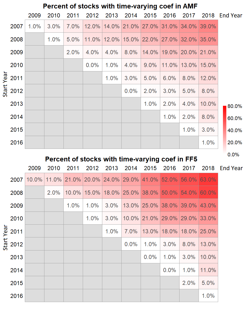
Figure 1: Percentage of stocks with time-varying beta using the time-invariance test in a linear setting for each time period. The y-axis is the start year of each time period and the x-axis is the end year. The percentage in each grid is the percentage of stocks with FDR Q-threshold 0.05 in Section 4.2 ANOVA test comparing the models in Equation (24) and (16).

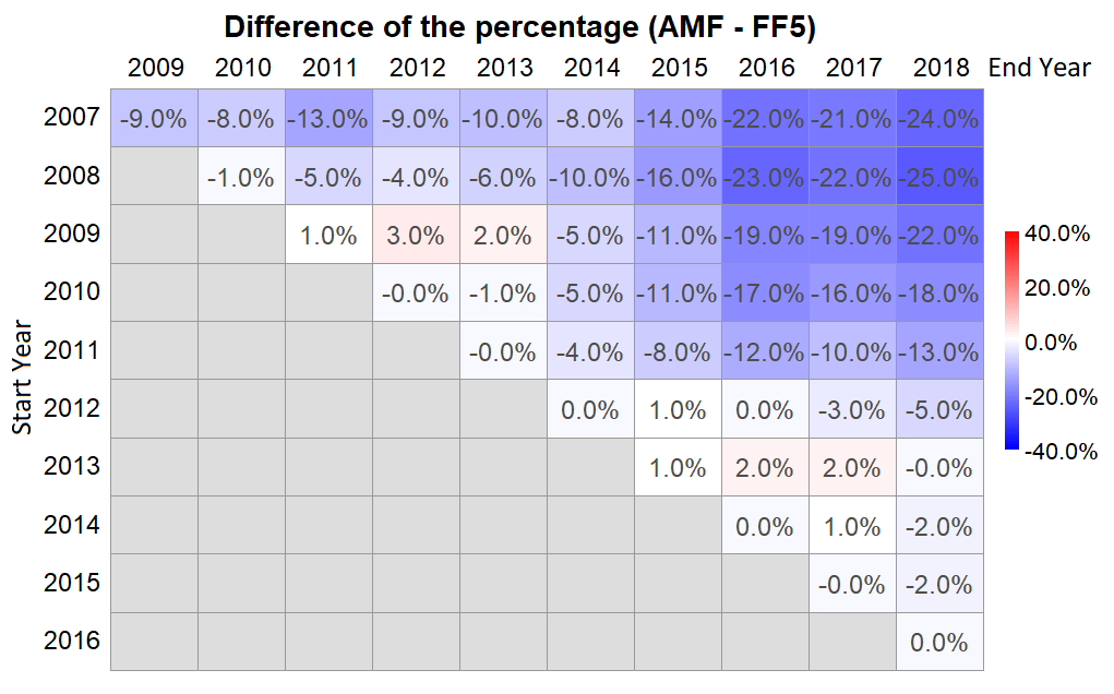
Figure 2: Difference of the two heatmaps in Figure 1 to compare AMF and FF5. Each grid is the percent of time-varying stocks in AMF model minus the percent of time-varying stocks in FF5 model shown in Figure 1.

In summary, AMF outperforms the FF5 in terms of the stability in two ways. First, for all time periods, AMF is more stable (or at least equally stable) than FF5, i.e. AMF either gives more stable $\beta$’s than FF5, or gives equally stable $\beta$’s if FF5 is also stable. Second, the stability of the AMF model for each time length is more robust across all mid-years as compared to FF5. The stability of the AMF model only depends on the length of the time period, and not the starting or ending year, while the stability of the FF5 model depends on the mid-year. This implies that the AMF performed well during the financial crisis.

4.3 Residual analysis

In this section we test if including more basis assets improves the fit in each time period. Since the number of ETFs increased over time, by focusing on the second half of the time period, we have more ETFs available compared to the beginning. We want to test if the newly introduced ETFs in the second half of the time period provides a better fit for the AMF model.

Formally, for a time period $[t_{a},t_{b}]$, let $t_{mid}=(t_{a}+t_{b})/2$. We divide $\Delta\bm{Y}_{i}$ and $\Delta\bm{V}$ into two parts, one for the time period $[t_{a},t_{mid})$ and the second for the time period $[t_{mid},t_{b})$, where

$$\Delta\bm{Y}_{i}=\begin{pmatrix}\Delta\bm{Y}_{i,a}\\ \Delta\bm{Y}_{i,b}\end{pmatrix},\quad\Delta\bm{V}=\begin{pmatrix}\Delta\bm{V}_{a}\\ \Delta\bm{V}_{b}\end{pmatrix}.$$ (26)

We first derive the basis assets set $S_{i}$ in Equation (15) using the GIBS algorithm on the whole time period. Then, we fit an OLS regression on the second half

$$\Delta\bm{Y}_{i,b}=(\Delta\bm{V}_{b})_{S_{i}}(\bm{\gamma}_{i})_{S_{i}}+\Delta\bm{\epsilon}_{i,b}$$ (27)

and obtain the estimated coefficients $(\bm{\hat{\gamma}}_{i})_{S_{i}}$. The residuals are

$$\Delta\bm{\hat{\epsilon}}_{i,b}=\Delta\bm{Y}_{i,b}-(\Delta\bm{V}_{b})_{S_{i}}(\bm{\hat{\gamma}}_{i})_{S_{i}}.$$ (28)

We fit an AMF model with the GIBS algorithm again, using the residuals $\Delta\bm{\hat{\epsilon}}_{i,b}$ as our new dependent variables, using all the basis assets available for the time period $[t_{mid},t_{b})$, except for the basis assets already selected in $S_{i}$. This AMF model on the residuals will provide another selected set of basis assets $S_{i,b}$. If $S_{i,b}\neq\emptyset$, we merge the two sets together

$$S_{i,union}=S_{i}\cup S_{i,b}.$$ (29)

Note that since we remove all the basis assets in $S_{i}$ in our GIBS fitting of the residuals, $S_{i}\cap S_{i,b}=\emptyset$. Continuing, we fit another OLS regression on the second half of the data using the basis assets $S_{i,union}$

$$\Delta\bm{Y}_{i,b}=(\Delta\bm{V}_{b})_{S_{i,union}}(\bm{\gamma}_{i})_{S_{i},union}+\Delta\bm{\epsilon}_{i,b}.$$ (30)

Finally, we use an ANOVA test to compare the models in Equation (27) and Equation (30). For each time period, this test is performed on all stocks yielding a list of p-values. As before, we adjust for FDR using the BHY [4] method and count the number of companies with FDR Q-values less than 0.05. The percentages are reported in Figure 3.

Note that if for $i$-th stock the set $S_{i,b}=\emptyset$, there will not be p-value for this stock since the two models in Equation (27) and (30) are the same. So this stock will not be counted as a company with a FDR Q-value less than 0.05. However, when presenting the percentage, we use the total count of companies available in that time period in the denominator. This generates more conservative percentages.

For the FF5 model, $S_{i}$ is the FF5 5-factors and the risk free rate. All the remaining steps in the procedure are the same. The results for FF5 residuals provide a comparison. From Figure 3 we see that for all time periods, the second half gives a significantly better fit with the new basis assets for around 15% of the stocks in the AMF model. Comparing this result with Figure 1, although there are stocks that have constant $\beta$’s, their risks can be better fitted using the new basis assets. This provides an interesting insight. More basis assets provides better fitting of the $\epsilon$ errors, although the affects of the old basis assets are still the same.

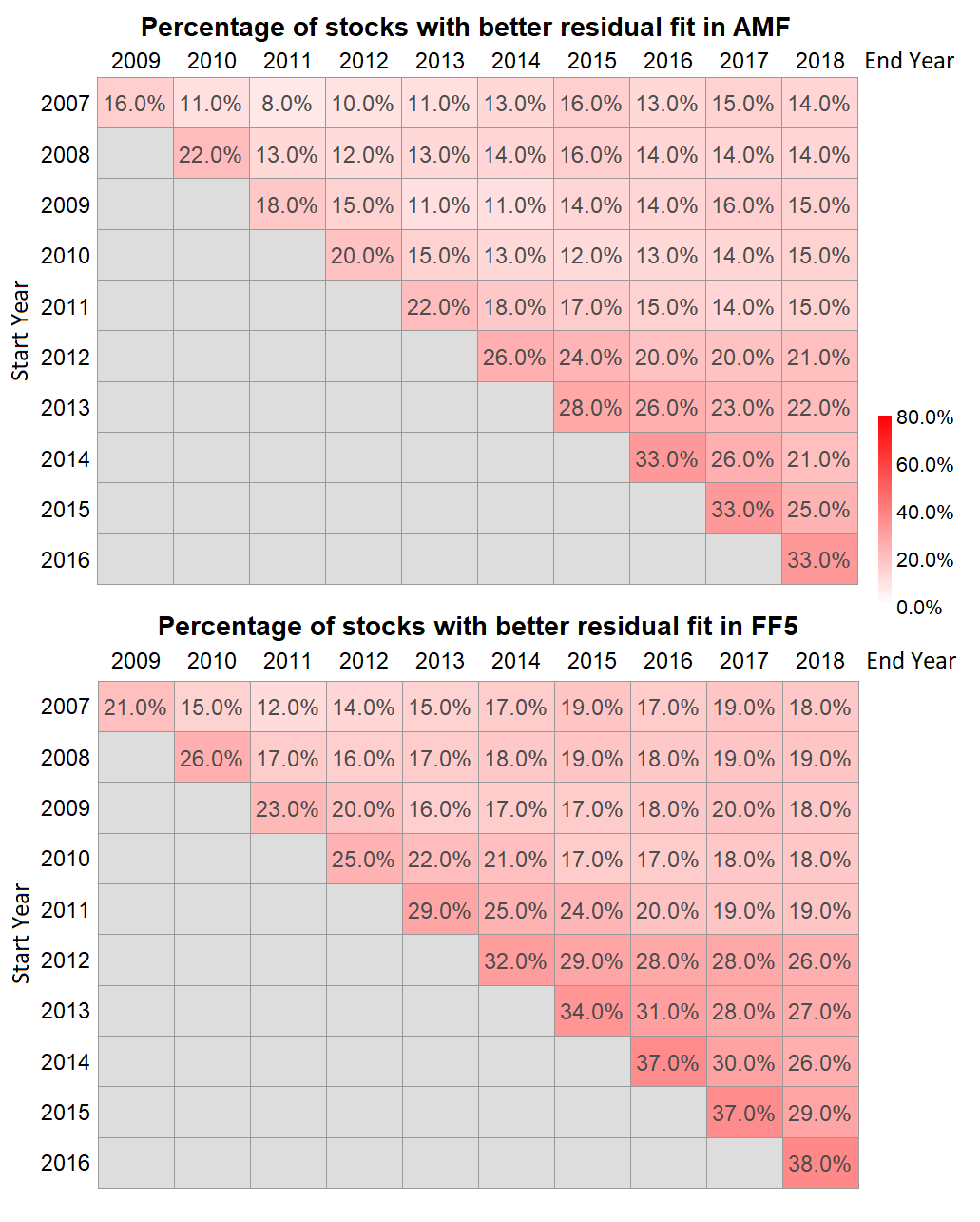
Figure 3: Percentage of stocks where the model in Equation (30) has significantly better fit compared to Equation (30) for each time period. The y-axis is the start year of each time period and the x-axis is the end year. The percentage in each grid is the percentage of stocks with FDR Q-threshold 0.05.

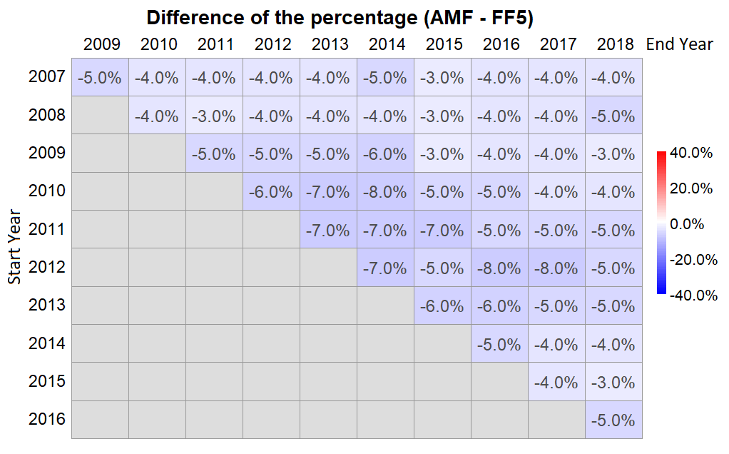
Figure 4: Difference of the two heatmaps in Figure 3. Each grid is the percentage in AMF model minus the percentage in FF5 model shown in Figure 3.

In summary, comparing the results for the AMF and FF5 residuals, it is clear that AMF uses more basis assets and leaves less information in the residuals than foes FF5. From Figure 4 we see that the percentage of stocks that are better fitted in the second half of the time period is always less for AMF than it is for FF5.

4.4 In-Sample and Out-of-Sample Goodness-of-Fit

This section reports the In-Sample and Out-of-Sample goodness-of-fit tests. Since the AMF selects more basis assets than the FF5, it is important to study overfitting. The results show that the AMF model is more powerful and less vulnerable to overfitting than is the FF5, because the AMF achieves a better in-sample Adjusted $R^{2}$ (see [20]) and a better Out-of-Sample $R^{2}$ (see [6]).

The Adjusted $R^{2}$ (see [20]) is a measure of goodness of fit similar to the normal $R^{2}$ but adjusted for the number of parameters to penalize on overfitting. The results are shown in Figure 5 and the difference of the Adjusted $R^{2}$ between AMF and FF5 is shown in Figure 6. It is clear that for all time periods, AMF increases the Adjsuted $R^{2}$ by around 0.1 compared to FF5, which is around a $0.1/0.25=40\%$ increment.

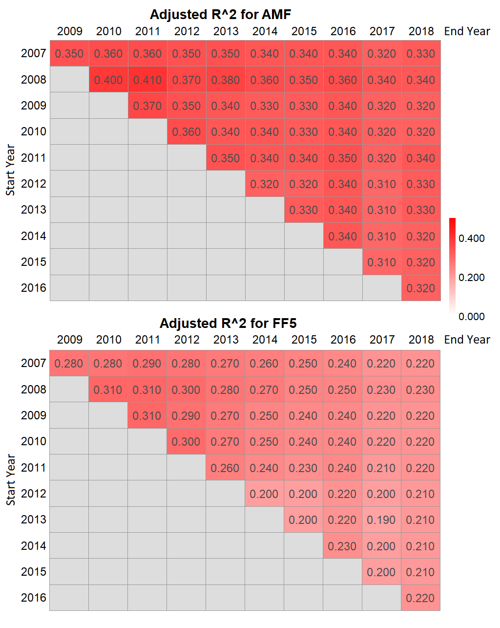
Figure 5: Mean Adjusted $R^{2}$ for the AMF and FF5 model. The y-axis is the start year of each time period and the x-axis is the end year.

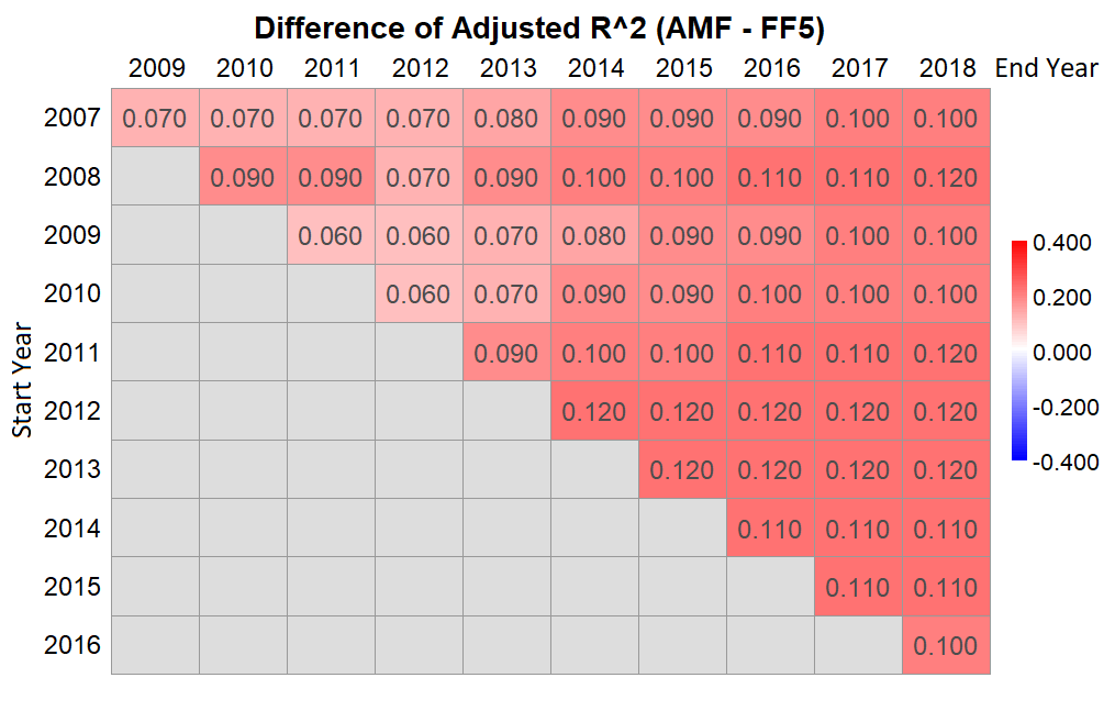
Figure 6: Difference of the two heatmaps in Figure 5. Each grid is the difference of the mean Adjusted $R^{2}$ of the AMF model minus that of the FF5 model shown in Figure 5.

The Out-of-Sample $R^{2}$ (see [6]) is a measure of a model’s prediction power. It can be used to check whether a model is overfitting. For each time period, we calculate the Out-of-Sample $R^{2}$ for AMF and FF5 for the half-year after the end of that period. The results are in Figure 7 and the differences of the Out-of-Sample $R^{2}$ between the two models are in Figure 8. We see that the prediction power of FF5 fades dramatically with time, while the prediction power of AMF is stable, and much better than the FF5. The Out-of-Sample $R^{2}$ for AMF is around 0.47, while that for FF5 is around 0.3 in early years and 0.2 in recent years. In recent years, the prediction power of the AMF model is almost twice as large as that of FF5. Therefore, it is clear that the basis assets selected by the AMF model are not overfitting, but achieving better in-sample and out-of-sample goodness-of-fit.

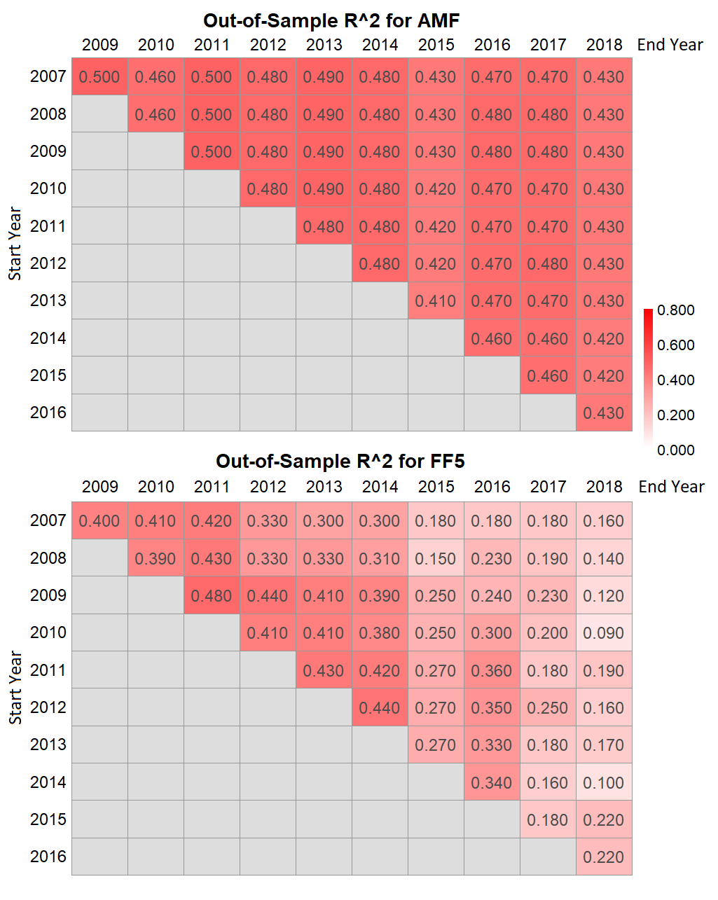
Figure 7: Mean Out-of-Sample $R^{2}$ for the AMF and FF5 model. The y-axis is the start year of each time period and the x-axis is the end year.

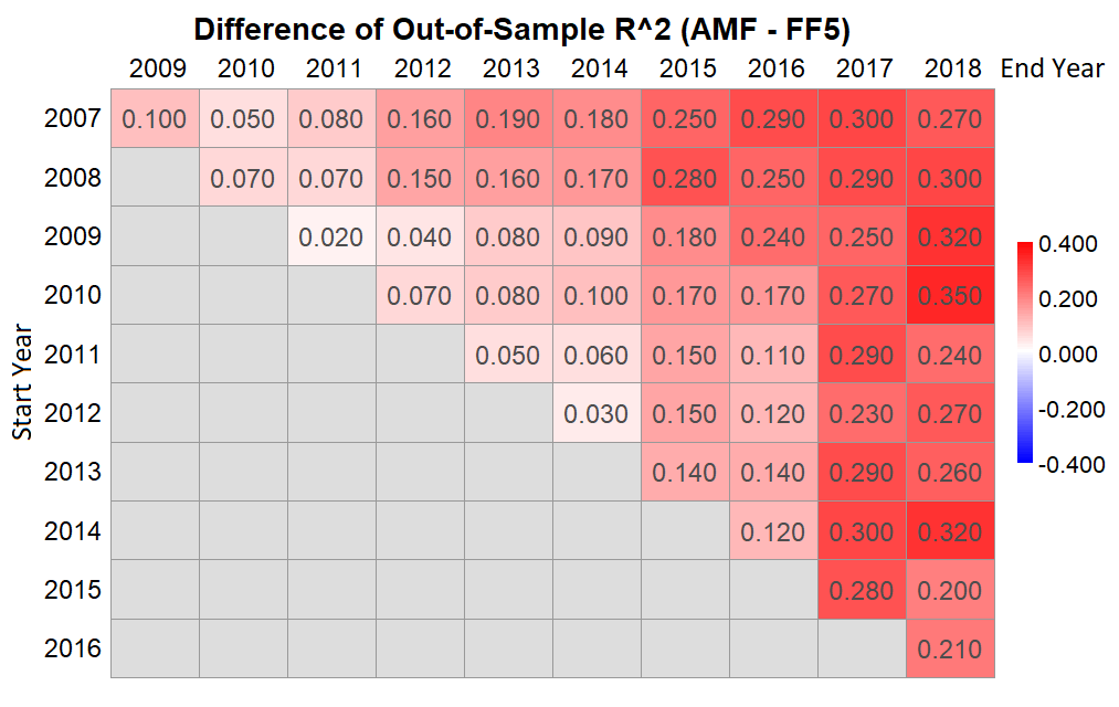
Figure 8: Difference of the two heatmaps in Figure 7. Each grid is the difference of the mean Out-of-Sample $R^{2}$ of the AMF model minus that of the FF5 model shown in Figure 7.

4.5 Time-invariance Test in Non-Linear GAM Setting

We can also test time-invariance based on thr non-linear Generalized Additive Model (GAM). This is a more strict test, since this tests not only for the time-invariance of the $\beta$’s, but also their linearity. We first fit a Time-Varying Coefficient model as a special case of the GAM. The equation can be written as:

$$\Delta\bm{Y}_{i}=\Delta\bm{V}_{S_{i}}[\bm{\beta}_{i}(t)]_{S_{i}}+\Delta\bm{\epsilon}_{i}$$ (31)

where $t$ is the time. Note that the only difference between Equation (31) and Equation (16) is the second allows the $\beta$’s to be functions of time $t$. The GAM model estimate each $\beta$ as a combination of splines or kernels with regard to $t$. This can be done by the gam() function in the R package mgcv.

Next, we perform a ANOVA test between the GAM model in Equation (31) and the linear model in Equation (16) where each $\bm{\beta}_{i}$ are constants over time. This yields a p-value for each stock. As before, we adjust the p-values using the BHY [4] method to account for FDR. We report the percentage of stocks with Q-values less than 0.05 in Figure 9.

Figure 9 reports the percentage of stocks with time-varying beta using the time-invariance test in a non-linear GAM setting for each time period. The y-axis is the start year and the x-axis is the end year of each time period. The percentage in each grid is the percentage of stocks with FDR Q-threshold 0.05 in the ANOVA test that compares the models in Equation (31) and (16). The larger the percentage, the darker the grid will be. The upper heatmap is for the AMF model, while the bottom heatmap is for the FF5 model.

By comparing the different skew-diagonals, we see that both models are more stable in shorter time periods. The AMF outperforms the FF5 in all the time periods, as seen in Figure 10. Figure 10 gives the difference between the percentages across the two heatmaps in Figure 9 (AMF - FF5). All the grids are blue, indicating that AMF is more stable than FF5 in all time periods.

However, comparing the results from GAM and the results from the previous Section 4.2, for any time period and both AMF and FF5 models, more companies are shown to have time-varying $\beta$’s in the GAM test, although the AMF still outperforms the FF5. This does not necessarily mean that the $\beta$’s are time varying in all time periods, since it is easy for GAM to overfit, especially in shorter time periods. Indeed, the number of observations for 3 year time periods is $n=156$. For the FF5 model, there are 5 basis assets. For the AMF model, there are more basis assets selected. For each basis asset, the GAM model selects some splines or kernels, say 10 splines, which can easily expand the dimension of parameters to $p=5\times 10=50$, which is already too large for a regression with $n=156$ observations. The number of parameters becomes too close to the number of observations. In addition, these new variables may be highly correlated, making the fitt more unstable. This can result in the GAM overfitting. Therefore, the testing based on the GAM model in this section is explorative. Considering this high-dimensional issue, penalization and constraints need to be introduced to traditional GAM for our application. This extension is left for future research.

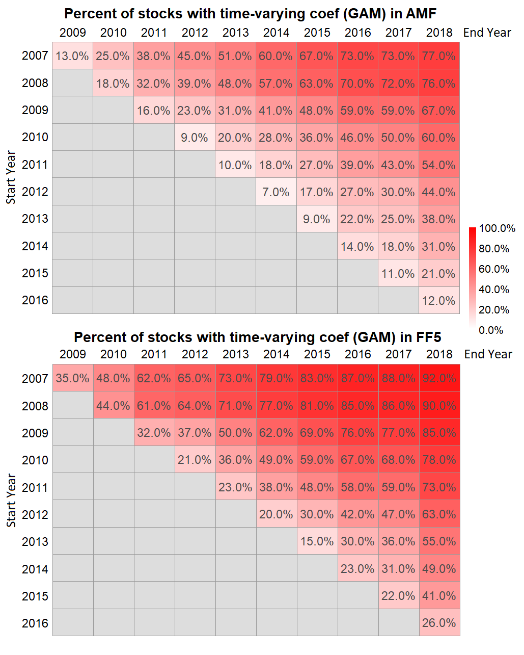
Figure 9: Percentage of stocks with time-varying beta using the time-invariance test in a non-linear GAM setting for each time period. The y-axis is the start year of each time period and the x-axis is the end year. The percentage in each grid is the percentage of stocks with FDR Q-threshold 0.05 in Section 4.2 ANOVA test comparing the models in Equation (31) and (16).

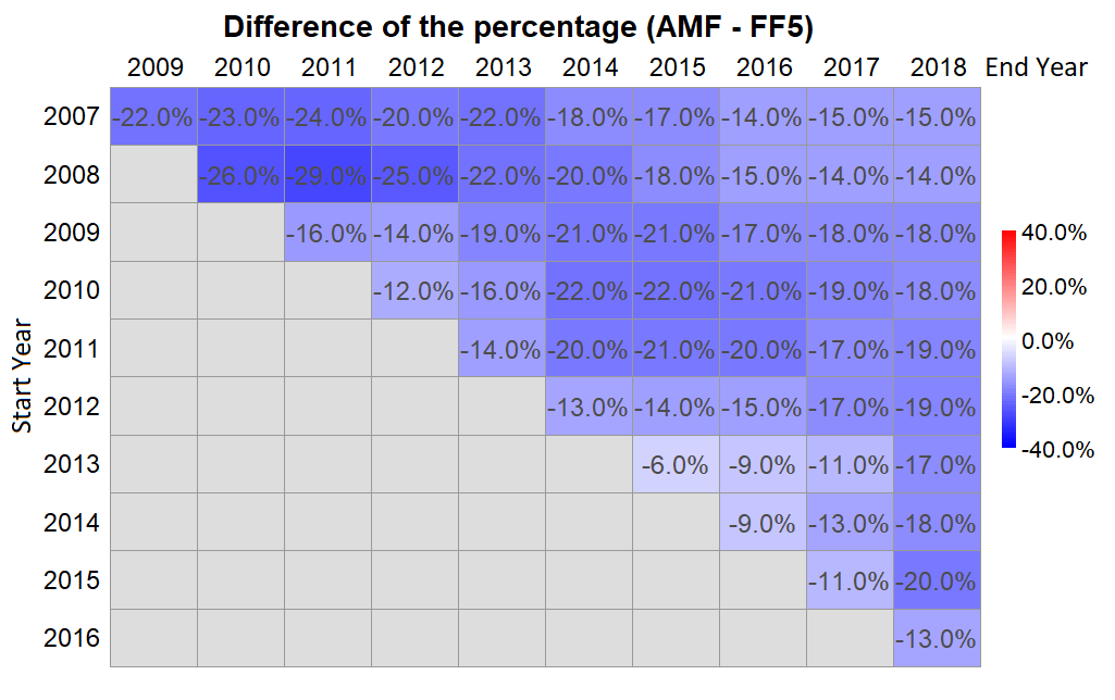
Figure 10: Difference of the two heatmaps in Figure 9 to compare AMF and FF5. Each grid is the percent of time-varying stocks in AMF model minus the percent of time-varying stocks in FF5 model shown inp Figure 9.

5 Conclusion

The purpose of this paper is to test the multi-factor beta model implied by the Generalized APT and the AMF model with the GIBS algorithm, without imposing the exogenous assumption of constant betas. The intercept (arbitrage) tests show that there is no significant non-zero intercepts in either AMF or FF5 model, which validates the 2 models. The in-sample and out-of-sample goodness-of-fit results show that AMF achieves both better in-sample adjusted $R^{2}$ and out-of-sample $R^{2}$, indicating that AMF is more powerful in fitting and less vulnerable to overfitting.

We perform time-invariance tests for the $\beta$’s for both the AMF and the FF5 models in various time periods. We show that the constant-beta assumption holds in the AMF model in all time periods with length less than 6 years and is quite robust regardless of the start year. However, even for short time periods, FF5 sometimes gives very unstable estimation, especially in financial crisis. This indicates that the AMF is more descriptive and it captures the basis assets that explain the market movements during the financial crisis. For time periods with length longer than 6 years, both AMF and FF5 fail to provide time-invariance $\beta$’s. However, the $\beta$’s estimate by the AMF is more time-invariant than the FF5 for nearly all time periods. This shows the superior performance of the AMF model. In summary, using the dynamic AMF model with a descent rolling window (such as 5 years) is more powerful and stable than is the FF5 model.

Appendix A Prototype Clustering and LASSO

This section describes the high-dimensional statistical methodologies used in the GIBS algorithm, including the prototype clustering and the LASSO. To remove unnecessary independent variables using clustering methods, we classify them into similar groups and then choose representatives from each group with small pairwise correlations. First, we define a distance metric to measure the similarity between points (in our case, the returns of the independent variables). Here, the distance metric is related to the correlation of the two points, i.e.

$$d(r_{1},r_{2})=1-|corr(r_{1},r_{2})|$$ (32)

where $r_{i}=(r_{i,t},r_{i,t+1},...,r_{i,T})^{\prime}$ is the time series vector for independent variable $i=1,2$ and $corr(r_{1},r_{2})$ is their correlation. Second, the distance between two clusters needs to be defined. Once a cluster distance is defined, hierarchical clustering methods (see [14]) can be used to organize the data into trees.

In these trees, each leaf corresponds to one of the original data points. Agglomerative hierarchical clustering algorithms (e.g. [14] [10]) build trees in a bottom-up approach, initializing each cluster as a single point, then merging the two closest clusters at each successive stage. This merging is repeated until only one cluster remains. Traditionally, the distance between two clusters is defined as either a complete distance, single distance, average distance, or centroid distance. However, all of these approaches suffer from interpretation difficulties and inversions (which means parent nodes can sometimes have a lower distance than their children), see Bien, Tibshirani (2011)[5]. To avoid these difficulties, Bien, Tibshirani (2011)[5] introduced hierarchical clustering with prototypes via a minimax linkage measure, defined as follows. For any point $x$ and cluster $C$, let

$$d_{max}(x,C)=\max_{x^{\prime}\in C}d(x,x^{\prime})$$ (33)

be the distance to the farthest point in $C$ from $x$. Define the minimax radius of the cluster $C$ as

$$r(C)=\min_{x\in C}d_{max}(x,C)$$ (34)

that is, this measures the distance from the farthest point $x\in C$ which is as close as possible to all the other elements in C. We call the minimizing point the prototype for $C$. Intuitively, it is the point at the center of this cluster. The minimax linkage between two clusters $G$ and $H$ is then defined as

$$d(G,H)=r(G\cup H).$$ (35)

Using this approach, we can easily find a good representative for each cluster, which is the prototype defined above. It is important to note that minimax linkage trees do not have inversions. Also, in our application as described below, to guarantee interpretable and tractability, using a single representative independent variable is better than using other approaches (for example, principal components analysis (PCA)) which employ linear combinations of the independent variables.

The LASSO method was introduced by Tibshirani (1996) [21] for model selection when the number of independent variables ($p$) is larger than the number of sample observations ($n$). The method is based on the idea that instead of minimizing the squared loss to derive the OLS solution for a regression, we should add to the loss a penalty on the absolute value of the coefficients to minimize the absolute value of the non-zero coefficients selected. To illustrate the procedure, suppose that we have a linear model

$$\bm{y}=\bm{X\beta}+\bm{\epsilon}\qquad\text{where}\qquad\bm{\epsilon}\sim N(0,\sigma_{\epsilon}^{2}\bm{I}),$$ (36)

$\bm{X}$ is an $n\times p$ matrix, $\bm{y}$ and $\bm{\epsilon}$ are $n\times 1$ vectors, and $\bm{\beta}$ is a $p\times 1$ vector.

The LASSO estimator of $\bm{\beta}$ is given by

$$\bm{\hat{\beta}}_{\lambda}=\underset{\bm{\beta}\in\mathbb{R}^{p}}{\arg\min}\left\{\frac{1}{2n}\left\|\bm{y}-\bm{X\beta}\right\|_{2}^{2}+\lambda\left\|\bm{\beta}\right\|_{1}\right\}$$ (37)

where $\lambda>0$ is the tuning parameter, which determines the magnitude of the penalty on the absolute value of non-zero $\beta$’s. In this paper, we use the R package glmnet [8] to fit LASSO.

In the subsequent estimation, we will only use a modified version of LASSO as a model selection method to find the collection of important independent variables. After the relevant basis assets are selected, we use a standard Ordinary Least-Square (OLS) regression on these variables to test for the goodness of fit and significance of the coefficients. More discussion of this approach can be found in Zhao, Shojaie, Witten (2017) [23].

In this paper, we fit the prototype clustering followed by a LASSO on the prototype basis assets selected. The theoretical justification for this approach can be found in Reid et al. (2018) [16] and Zhao et al. (2017) [23].

Appendix B ETF Classes and Subclasses

ETFs can be divided into 10 classes, 73 subclasses (categories) in total, based on their financial explanations. The classify criteria are found from the ETFdb database: www.etfdb.com. The classes and subclasses are listed below:

1. Bond/Fixed Income: California Munis, Corporate Bonds, Emerging Markets Bonds, Government Bonds, High Yield Bonds, Inflation-Protected Bonds, International Government Bonds, Money Market, Mortgage Backed Securities, National Munis, New York Munis, Preferred Stock/Convertible Bonds, Total Bond Market.

2. Commodity: Agricultural Commodities, Commodities, Metals, Oil & Gas, Precious Metals.

3. Currency: Currency.

4. Diversified Portfolio: Diversified Portfolio, Target Retirement Date.

5. Equity: All Cap Equities, Alternative Energy Equities, Asia Pacific Equities, Building & Construction, China Equities, Commodity Producers Equities, Communications Equities, Consumer Discretionary Equities, Consumer Staples Equities, Emerging Markets Equities, Energy Equities, Europe Equities, Financial Equities, Foreign Large Cap Equities, Foreign Small & Mid Cap Equities, Global Equities, Health & Biotech Equities, Industrials Equities, Japan Equities, Large Cap Blend Equities, Large Cap Growth Equities, Large Cap Value Equities, Latin America Equities, MLPs (Master Limited Partnerships), Materials, Mid Cap Blend Equities, Mid Cap Growth Equities, Mid Cap Value Equities, Small Cap Blend Equities, Small Cap Growth Equities, Small Cap Value Equities, Technology Equities, Transportation Equities, Utilities Equities, Volatility Hedged Equity, Water Equities.

6. Alternative ETFs: Hedge Fund, Long-Short.

7. Inverse: Inverse Bonds, Inverse Commodities, Inverse Equities, Inverse Volatility.

8. Leveraged: Leveraged Bonds, Leveraged Commodities,
   Leveraged Currency, Leveraged Equities, Leveraged Multi-Asset, Leveraged Real Estate, Leveraged Volati-lity.

9. Real Estate: Global Real Estate, Real Estate.

10. Volatility: Volatility.

References

- [1] Tobias Adrian, Richard K Crump, and Emanuel Moench. Regression based estimation of dynamic asset pricing models. Journal of Financial Economics, 118(2):211–244, 2015.
- [2] Doron Avramov and Tarun Chordia. Asset pricing models and financial market anomalies. The Review of Financial Studies, 19(3):1001–1040, 2006.
- [3] Yoav Benjamini and Yosef Hochberg. Controlling the false discovery rate: a practical and powerful approach to multiple testing. Journal of the Royal Statistical Society: Series B (Methodological), 57(1):289–300, 1995.
- [4] Yoav Benjamini and Daniel Yekutieli. The control of the false discovery rate in multiple testing under dependency. The Annals of Statistics, 29(4):1165–1188, 2001.
- [5] Jacob Bien and Robert Tibshirani. Hierarchical clustering with prototypes via minimax linkage. Journal of the American Statistical Association, 106(495):1075–1084, 2011.
- [6] John Y Campbell and Samuel B Thompson. Predicting excess stock returns out of sample: Can anything beat the historical average? The Review of Financial Studies, 21(4):1509–1531, 2008.
- [7] Ilan Cooper and Paulo Maio. New evidence on conditional factor models. Journal of Financial and Quantitative Analysis, 54(5):1975–2016, 2019.
- [8] Jerome Friedman, Trevor Hastie, and Rob Tibshirani. Regularization paths for generalized linear models via coordinate descent. Journal of Statistical Software, 33(1):1, 2010.
- [9] Campbell R Harvey, Yan Liu, and Heqing Zhu. . . . and the cross-section of expected returns. The Review of Financial Studies, 29(1):5–68, 2016.
- [10] Xiao Huang, Zhenlong Li, Junyu Lu, Sicheng Wang, Hanxue Wei, and Baixu Chen. Time-series clustering for home dwell time during covid-19: what can we learn from it? ISPRS International Journal of Geo-Information, 9(11):675, 2020.
- [11] Ravi Jagannathan, Ernst Schaumburg, and Guofu Zhou. Cross-sectional asset pricing tests. Annual Review of Financial Economics, 2(1):49–74, 2010.
- [12] Robert Jarrow and Philip Protter. Positive alphas and a generalized multiple-factor asset pricing model. Mathematics and Financial Economics, 10(1):29–48, 2016.
- [13] Robert A Jarrow, Rinald Murataj, Martin T Wells, and Liao Zhu. The low-volatility anomaly and the adaptive multi-factor model. arXiv preprint arXiv:2003.08302, 2021.
- [14] Leonard Kaufman and Peter J Rousseeuw. Finding Groups in Data: An Introduction to Cluster Analysis, volume 344. John Wiley & Sons, 2009.
- [15] Robert C Merton. An intertemporal capital asset pricing model. Econometrica: Journal of the Econometric Society, 41(5):867–887, 1973.
- [16] Stephen Reid, Jonathan Taylor, and Robert Tibshirani. A general framework for estimation and inference from clusters of features. Journal of the American Statistical Association, 113(521):280–293, 2018.
- [17] Stephen A Ross. The arbitrage theory of capital asset pricing. Journal of Economic Theory, 13(3):341–360, 1976.
- [18] Tyler Shumway. The delisting bias in crsp data. The Journal of Finance, 52(1):327–340, 1997.
- [19] Noah Simon, Jerome Friedman, Trevor Hastie, and Rob Tibshirani. Regularization paths for cox’s proportional hazards model via coordinate descent. Journal of Statistical Software, 39(5):1, 2011.
- [20] Henri Theil. Economic Forecasts and Policy. North-Holland Pub. Co., 1961.
- [21] Robert Tibshirani. Regression shrinkage and selection via the lasso. Journal of the Royal Statistical Society: Series B (Methodological), 58(1):267–288, 1996.
- [22] Robert Tibshirani, Jacob Bien, Jerome Friedman, Trevor Hastie, Noah Simon, Jonathan Taylor, and Ryan J Tibshirani. Strong rules for discarding predictors in lasso-type problems. Journal of the Royal Statistical Society: Series B (Statistical Methodology), 74(2):245–266, 2012.
- [23] Sen Zhao, Ali Shojaie, and Daniela Witten. In defense of the indefensible: A very naive approach to high-dimensional inference. arXiv preprint arXiv:1705.05543, 2017.
- [24] Liao Zhu, Sumanta Basu, Robert A. Jarrow, and Martin T. Wells. High-dimensional estimation, basis assets, and the adaptive multi-factor model. The Quarterly Journal of Finance, 10(04):2050017, 2020.