Likelihood Inference for Possibly Non-Stationary Processes via Adaptive Overdifferencing

Abstract

We make an observation that facilitates exact likelihood-based inference for the parameters of the popular ARFIMA model without requiring stationarity by allowing the upper bound $\bar{d}$ for the memory parameter $d$ to exceed $0.5$. We observe that estimating the parameters of a single non-stationary ARFIMA model is equivalent to estimating the parameters of a sequence of stationary ARFIMA models, which allows for the use of existing methods for evaluating the likelihood for an invertible and stationary ARFIMA model. This enables improved inference because many standard methods perform poorly when estimates are close to the boundary of the parameter space. It also allows us to leverage the wealth of likelihood approximations that have been introduced for estimating the parameters of a stationary process. We explore how estimation of the memory parameter $d$ depends on the upper bound $\bar{d}$ and introduce adaptive procedures for choosing $\bar{d}$. Via simulations, we examine the performance of our adaptive procedures for estimating the memory parameter when the true value is as large as $2.5$. Our adaptive procedures estimate the memory parameter well, can be used to obtain confidence intervals for the memory parameter that achieve nominal coverage rates, and perform favorably relative to existing alternatives.

Keywords: long memory; ARFIMA; FARIMA

1 Introduction

Many methods for analyzing an equally spaced time series $\boldsymbol{y}=\left(y_{1},\dots,y_{n}\right)$ have been developed. Stationary autoregressive moving average (ARMA) models and their non-stationary generalizations predominate. An ARMA$\left(p,q\right)$ model assumes that deviations of observations $y_{t}$ from their means $\mu_{t}$ are a function of past deviations and stochastic errors,

$$\phi\left(B\right)\left(y_{t}-\mu_{t}\right)=\theta\left(B\right)z_{t}\text{, \quad}z_{t}\stackrel{{\scriptstyle i.i.d.}}{{\sim}}\mathcal{N}\left(0,\sigma^{2}\right),$$ (1)

where $\phi\left(B\right)=1-\sum_{\ell=1}^{p}\phi_{\ell}B^{\ell}$, $\theta\left(B\right)=1+\sum_{\ell=1}^{q}\theta_{\ell}B^{\ell}$, and $B$ is the shift $B^{\ell}y_{t}=y_{t-\ell}$. The mean $\mu_{t}$ is a specified function of a small number of unknown parameters, and may be assumed to be an unknown constant, a low degree polynomial function in time $t$ with unknown coefficients, or a linear function of a small number of predictors with unknown coefficients. Equation (1) describes a stationary, causal, and invertible model when all roots of the autoregressive polynomial $\phi\left(z\right)$ and all roots of the moving average polynomial $\theta\left(z\right)$ lie outside of the unit circle. Stationarity ensures that the mean and variance of the deviations $y_{t}-\mu_{t}$ are constant over time and that correlations between deviations depend only on how far apart they are in time. Further, the autocorrelation function uniquely determines the ARMA$\left(p,q\right)$ parameters. An autoregressive moving average (ARIMA) model generalizes the ARMA model to allow for certain types of non-stationarity , specifically the presence of certain deterministic time trends (Box and Jenkins, 1970). An ARIMA$\left(p,d,q\right)$ model assumes that there is a nonnegative integer $d$ such that the $d$-th differences $\left(1-B\right)^{d}\left(y_{t}-\mu_{t}\right)$ satisfy the ARMA$\left(p,q\right)$ equation. Thus, the ARIMA$\left(p,d,q\right)$ model is equivalent to assuming an ARMA$\left(p,q\right)$ model for deviations of a simple function of observations from their means $\left(1-B\right)^{d}\mu_{t}$, which can allow for the presence of certain deterministic trends without estimating them because $\left(1-B\right)^{d}\mu_{t}=0$ when $\mu_{t}=\sum_{j=0}^{d-1}t^{j}\lambda_{j}$.

Stationary ARMA$\left(p,q\right)$ models are not well suited for modeling correlations that decay very slowly over time because slowly decaying correlations require ARMA$\left(p,q\right)$ models with an increasing number of parameters as the length of the time series grows (Granger, 1980). For this purpose, long memory or autoregressive fractionally differenced moving average (ARFIMA or FARIMA) models have been developed (Hosking, 1981; Granger, 1980). An ARFIMA$\left(p,d,q\right)$ model assumes that a fractional difference of the deviations $\left(1-B\right)^{d}\left(y_{t}-\mu_{t}\right)$ is distributed according to a stationary ARMA$\left(p,q\right)$ model where

$$\left(1-B\right)^{d}=\sum_{\ell=0}^{\infty}{d\choose\ell}\left(-1\right)^{\ell-1}B^{\ell}.$$ (2)

This describes a stationary and invertible ARFIMA$\left(p,d,q\right)$ model when $-1<d<0.5$ (Odaki, 1993). An ARFIMA$\left(p,d,q\right)$ process has slowly decaying correlations when $d>0$, because each deviation $y_{t}-\mu_{t}$ depends on infinitely many past deviations and the corresponding weights decay slowly. The ARIMA$\left(p,d,q\right)$ model is obtained when $d$ is an integer. Such models are fit to the data by first differencing the data an appropriate number of times, and fitting a stationary model to the differenced deviations.

Accordingly, one common approach for maximum likelihood estimation of possibly non-stationary ARFIMA$\left(p,d,q\right)$ models is to decide how much to difference the data first by finding the smallest integer $k$ for which $\left(1-B\right)^{k}\left(y_{t}-\mu_{t}\right)$ appears to be stationary, and assuming a stationary ARFIMA$\left(p,d,q\right)$ model for the differenced deviations $\left(1-B\right)^{k}\left(y_{t}-\mu_{t}\right)$ for $-0.5<d<0.5$. This approach is described in Hualde and Robinson (2011) and intuitively called the “difference-and-add-back” approach by Johansen and Nielsen (2016); it has been recommended by Box-Steffensmeier and Smith (1998) and used in practice (Byers et al., 1997, 2000; Dolado et al., 2003). Although useful, this procedure can lead to practical challenges in the presence of nearly non-stationary differenced ARFIMA$\left(p,d,q\right)$ processes, which are processes that are well represented by values of $d$ close to the boundary of stationarity of the differenced processes, e.g. $d\approx 0.5$, $d\approx 1.5$, or $d\approx 2.5$. Furthermore, it can be difficult to decide whether or not a stationary model is reasonable for an observed time series with slowly decaying empirical correlations.

Figure 1 illustrates this with two time series of length $n=500$. Both time series are simulated according to an ARFIMA$\left(0,d,0\right)$ model $\left(1-B\right)^{d}y_{t}=z_{t}$ using the same stochastic errors $z_{t}$ simulated from a standard normal distribution. The first is simulated according to a stationary process with $d=0.45$ and the second is stimulated according to a non-stationary process with $d=0.55$. The latter time series is simulated by taking cumulative sums of time series simulated according to a stationary process. Although the first time series is simulated from a stationary model and the second is not, both observed time series and their corresponding sample autocorrelation functions look similar.

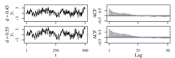
Figure 1: Simulated length $n=500$ time series and their sample autocorrelation functions (ACFs). Both time series satisfy the ARFIMA$\left(0,d,0\right)$ model with $\mu=0$ and the same stochastic errors with memory parameter $d=0.45$ or $d=0.55$. For reference, approximate 95% intervals for sample autocorrelations of a white noise process are provided with ACFs.

Despite the fact that the stationary and non-stationary time series shown in Figure 1 look similar, the likelihoods of the two time series under an ARIMA$\left(0,d-k,0\right)$ model for the deviations $y_{t}-\mu$ obtained using the “difference-and-add-back” approach of fitting a stationary ARIMA$\left(0,d-k,0\right)$ model to the $k$-th differenced data $\left(1-B\right)^{k}\left(y_{t}-\mu\right)$ for $-0.5<d-k<0.5$ are not continuous at $d=k+0.5$; see Figure 2. This is because the data changes from the $n$ observed time series values to the $n-1$ observed differences when we evaluate the likelihood for $d>0.5$. For this reason, likelihood values obtained in this way are of limited utility. They are only comparable across subsets of $d$ values that correspond to the same amount of differencing. Furthermore, the presence of boundaries and discontinuities can produce misleading standard errors and confidence intervals for estimates of the memory parameter $d$, whether they are based on asymptotic or bootstrap methods. A possible solution is suggested by recognizing that $\left(1-B\right)^{d}\left(y_{t}-\mu\right)=\left(1-B\right)^{d-k}\left(1-B\right)^{k}\left(y_{t}-\mu\right)$. Thus, if $y_{t}-\mu$ is an ARFIMA$\left(0,d,0\right)$ process, then the $k$-th difference $\left(1-B\right)^{k}\left(y_{t}-\mu\right)$ is an ARFIMA$\left(0,d-k,0\right)$ process. However, an ARFIMA$\left(0,d-k,0\right)$ process is only invertible for $d>k-1$. Although consistency and asymptotic normality of the maximum likelihood estimator of the memory parameter $d$ has been shown for all $d<k+0.5$ (Lieberman et al., 2012), careful examination of the references in and of Lieberman et al. (2012) yields no examples of maximum likelihood estimators that allow for $d-k$ outside of the invertible range, $d\leq k-1$.

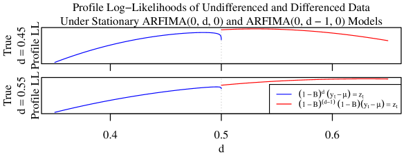
Figure 2: Profile log-likelihoods of undifferenced and first-differenced data under an ARFIMA$\left(0,d,0\right)$ with $\mu_{t}=\mu$ and $\sigma^{2}$ profiled for the time series shown in Figure 1.

Instead, existing alternative solutions are based on approximate likelihoods. The conditional sum-of-squares (CSS) approximate likelihood, as described in Beran (1995), Hualde and Robinson (2011), and Hualde and Nielsen (2020), uses the truncated fractional difference $\left(1-B\right)^{d}_{+}\left(y_{t}-\mu\right)=\sum_{\ell=0}^{t-1}{d\choose\ell}\left(-1\right)^{\ell-1}B^{\ell}\left(y_{t}-\mu\right)$ to approximate $\left(1-B\right)^{d}\left(y_{t}-\mu\right)$ and obtain an approximate likelihood that is continuous in $d$. Hualde and Robinson (2011) and Hualde and Nielsen (2020) proved that the CSS approximate likelihood provides consistent, asymptotically normal parameter estimates under a slightly modified model where the truncated fractional difference of the data $\left(1-B\right)^{d}_{+}\left(y_{t}-\mu_{t}\right)=\sum_{\ell=0}^{t-1}{d\choose\ell}\left(-1\right)^{\ell-1}B^{\ell}\left(y_{t}-\mu_{t}\right)$ is distributed according to a stationary ARMA$\left(p,q\right)$ model with $\mu_{t}=\mu_{0}\left(t\mathbbm{1}_{\left\{t\geq 1\right\}}\right)^{\gamma_{0}}$ for unknown $\mu_{0}$ and $\gamma_{0}$. However, it is known that these CSS approximate likelihood based estimates can be more biased than exact likelihood based estimates in finite samples if the data is generated according to an ARFIMA$\left(p,d,q\right)$ process (Johansen and Nielsen, 2016). Other alternatives involve the specification of additional tuning parameters. Velasco and Robinson (2000) introduced spectral methods for $-0.5<d$ and Hurvich and Chen (2000) introduced spectral methods that have the added benefit of being invariant to the presence of linear trends for $-0.5<d<1.5$. The estimators introduced in Velasco and Robinson (2000) depend on the tapering applied to the sample periodogram and both the estimators introduced in both Velasco and Robinson (2000) and Hurvich and Chen (2000) require specification of the number of periodogram ordinates used for estimation of the ARFIMA$\left(p,d,q\right)$ parameters. More recently, Mayoral (2007) introduced a moment-based method for $d>-0.75$ based on the first $k$ sample autocorrelations, however it also requires the specification of the number of sample autocorrelations to be considered. None of these references introducing and exploring approximate likelihood-based solutions include comparisons to exact likelihood-based estimators that allow for estimates of the memory parameter outside of the stationary and invertible range.

This paper shows that given an upper bound $\bar{d}$ for the memory parameter $d$, it is possible to implement exact likelihood estimation for differenced data for all $d<\bar{d}$. Our approach is motivated by the earlier observation that the $k$-th difference of an ARFIMA$\left(0,d,0\right)$ process is a ARFIMA$\left(0,d-k,0\right)$ process and the literature showing consistency and asymptotic normality of exact likelihood estimators of ARFIMA$\left(0,d-k,0\right)$ models for all $d-k<0.5$ (Lieberman et al., 2012). Given an upper bound $\bar{d}$, we can difference the data before estimation and reduce the problem of estimating the parameters of a single non-stationary ARFIMA$\left(p,d,q\right)$ model to the problem of estimating the parameters of a sequence of stationary ARFIMA$\left(p,d,q\right)$ models with constrained moving average parameters. The upper bound $\bar{d}$ can be selected adaptively without a priori knowledge of the process’ stationarity.

This paper proceeds as follows. First, we explain how the problem of estimating the parameters of a possibly non-stationary ARFIMA$\left(p,d,q\right)$ model with memory parameter $d$ bounded above by a fixed value $\bar{d}$ can be transformed to a simpler problem of estimating the parameters of a sequence of stationary ARFIMA$\left(p,d,q\right)$ models with constrained moving average parameters that correspond to a non-invertible moving average process, with likelihoods that can then be related to the likelihoods of invertible and stationary ARFIMA$\left(p,d,q\right)$ models. We then introduce adaptive procedures for choosing $\bar{d}$. We demonstrate the need for and performance of the adaptive procedures based on the exact likelihood and the approximate likelihoods for ARFIMA$\left(0,d,0\right)$ processes in simulations. We show that the adaptive procedures can produce estimates of $d$ with low bias and, when based on the exact likelihood, confidence intervals with nominal coverage. We also compare the bias of adaptive exact likelihood estimators to the two alternatives described in Beran (1995) and introduced in Mayoral (2007). We observe comparable performance to alternatives when $n$ is relatively small and better performance than the alternatives as $n$ increases when long memory is present. We use the proposed methods to fit possibly non-stationary ARFIMA$\left(1,d,0\right)$ and ARFIMA$\left(0,d,1\right)$ models to time series featured in the literature, and discuss the challenges of estimating the parameters of possibly non-stationary ARFIMA$\left(p,d,q\right)$ models with $p>0$ or $q>0$ in practice. We apply the proposed methods to an existing problem which uses tests of non-stationarity of ARFIMA$\left(0,d,0\right)$ models for deviations from a linear trend to assess mean reversion of OECD countries’ per capita CO₂ emissions. Last, we apply the proposed methods to pooled estimation of ARFIMA$\left(0,d,0\right)$ models from electric cell-substrate impedance sensing (ECIS) measurements.

2 Methodology

2.1 Relating Non-Stationary to Stationary Problems Given $\bar{d}$

Let $y_{t}-\mu_{t}$ be a possibly non-stationary ARFIMA$\left(p,d,q\right)$ process with autoregressive parameters $\boldsymbol{\phi}=\left(\phi_{1},\dots,\phi_{p}\right)$ and moving average parameters $\boldsymbol{\theta}=\left(\theta_{1},\dots,\theta_{q}\right)$ satisfying

$$\phi\left(B\right)\left(1-B\right)^{d}\left(y_{t}-\mu_{t}\right)=\theta\left(B\right)z_{t}\text{, \quad}z_{t}\stackrel{{\scriptstyle i.i.d.}}{{\sim}}\mathcal{N}\left(0,\sigma^{2}\right),$$ (3)

where all roots of $\phi\left(z\right)$ and $\theta\left(z\right)$ lie outside of the unit circle and $d<\bar{d}$ for some $\bar{d}\geq 0.5$. Deviations of the differenced process $x^{\left(m\right)}_{t}=\left(1-B\right)^{m}y_{t}$ from their means $\mu^{\left(m\right)}_{t}=\left(1-B\right)^{m}\mu_{t}$ are stationary for any $m$ satisfying $\bar{d}-m<0.5$ and can be computed exactly for $t>m$ if $m$ is an integer. Let $m_{\bar{d}}$ be the smallest integer that satisfies $\bar{d}-m_{\bar{d}}\leq 0.5$.

Having found an integer $m_{\bar{d}}$ satisfying $\bar{d}-m_{\bar{d}}\leq 0.5$, we can evaluate the likelihood of the differenced deviations $l_{\bar{d}}\left(\boldsymbol{x}^{\left(m_{\bar{d}}\right)}|d,\mu_{t},\sigma,\boldsymbol{\theta},\boldsymbol{\phi}\right)$ for $d<\bar{d}$ (Hosking, 1981). When the differenced mean is constant, $\mu^{\left(m\right)}_{t}=\mu$, the maximum likelihood estimator of $d$ based on the differenced deviations will be consistent and asymptotically normal for $d<\bar{d}$ (Lieberman et al., 2012). This procedure can produce estimates of the memory parameter over the interval $d<\bar{d}$ that are invariant to polynomial trends of degree $m$ or lower, depending on the assumed mean $\mu_{t}$. The estimator obtained by setting $\bar{d}=1.5$ and $\mu_{t}=\lambda_{0}+\lambda_{1}t$ is invariant to linear trends, and the estimator obtained by setting $\bar{d}=2.5$ and $\mu_{t}=\sum_{j=0}^{2}t^{j}\lambda_{j}$ is invariant to quadratic trends. This is a benefit when polynomial trends are a nuisance and a limitation polynomial trends are themselves of interest.

Despite theoretical justifications of maximum likelihood estimation for $d<\bar{d}$ (Lieberman et al., 2012), maximum likelihood estimation of a stationary ARFIMA$\left(p,d,q\right)$ process tends to require $\bar{d}-1\leq d<\bar{d}$. (Pipiras and Taqqu, 2017; Durham et al., 2019). This ensures that the likelihood is only evaluated for parameters that correspond to an invertible process for the differenced deviations. It also allows for the use of certain efficient methods for evaluating the autocovariances of the differenced deviations which require $\bar{d}-1\leq d<\bar{d}$ which are essential because evaluating the autocovariances of an ARFIMA$\left(p,d,q\right)$ process is computationally burdensome (Doornik and Ooms, 2003), e.g. the methods of Sowell (1992). This motivates rewriting the model as

$$\phi\left(B\right)\left(1-B\right)^{d-m_{\bar{d}}+j}\left(x^{\left(m_{\bar{d}}\right)}_{t}-\mu^{\left(m_{\bar{d}}\right)}_{t}\right)=\left(1-B\right)^{j}\theta\left(B\right)z_{t}\text{, \quad}z_{t}\stackrel{{\scriptstyle i.i.d.}}{{\sim}}\mathcal{N}\left(0,\sigma^{2}\right),$$ (4)

where $j$ is a nonnegative integer satisfying $-0.5\leq d-m_{\bar{d}}+j<0.5$. This is a stationary ARFIMA$\left(p,d-m_{\bar{d}}+j,j+q\right)$ model for the differenced deviations with $j+q$ constrained moving average parameters $\tilde{\theta}_{1}^{\left(j\right)},\dots,\tilde{\theta}^{\left(j\right)}_{j+q}$ obtained by expanding out $\left(1-B\right)^{j}\theta\left(B\right)$. It is non-invertible for $j>0$; the moving average polynomial $\tilde{\theta}\left(B\right)$ has roots on the unit circle.

The advantage of rewriting the model is that the covariance $\boldsymbol{\Gamma}_{n-m_{\bar{d}}}\left(d-m_{\bar{d}}+j,\tilde{\boldsymbol{\theta}},\boldsymbol{\phi},\sigma\right)$ of $n-m_{\bar{d}}$ differenced deviations under the ARFIMA$\left(p,d-m_{\bar{d}}+j,j+q\right)$ model (4) is

$$\boldsymbol{\Gamma}_{n-m_{\bar{d}}}\left(d-m_{\bar{d}}+j,\tilde{\boldsymbol{\theta}},\boldsymbol{\phi},\sigma\right)=\boldsymbol{A}_{\bar{d}\left(j\right)}\boldsymbol{\Omega}_{n-m_{\bar{d}}+j}\left(d-m_{\bar{d}}+j,\boldsymbol{\theta},\boldsymbol{\phi},\sigma\right)\boldsymbol{A}_{\bar{d}\left(j\right)}^{\prime},$$ (5)

where $\boldsymbol{A}_{\bar{d}\left(j\right)}$ is the $\left(n-m_{\bar{d}}\right)\times\left(n-m_{\bar{d}}+j\right)$ $j$-th differencing matrix that returns $n-m_{\bar{d}}$ $j$-th differences and $\boldsymbol{\Omega}_{n-m_{\bar{d}}+j}\left(d-m_{\bar{d}}+j,\boldsymbol{\theta},\boldsymbol{\phi},\sigma\right)$ is the $\left(n-m_{\bar{d}}+j\right)\times\left(n-m_{\bar{d}}+j\right)$ covariance matrix for a stationary and invertible ARFIMA$\left(p,d-m_{\bar{d}}+j,q\right)$ process with moving average and autoregressive parameters $\boldsymbol{\theta}$ and $\boldsymbol{\phi}$ and standard deviation $\sigma$. As a result, any method for obtaining autocovariances of a stationary and invertible ARFIMA$\left(p,d,q\right)$ process can be used to obtain the autocovariances needed to compute the likelihood of $\boldsymbol{x}^{\left(m_{\bar{d}}\right)}-\boldsymbol{\mu}^{\left(m_{\bar{d}}\right)}$. Furthermore, autocovariances can be reused across multiple values of $j$.

Given an upper bound $\bar{d}$ the ARFIMA$\left(p,d,q\right)$ likelihood can be obtained as a function of the unknown parameters of the mean $\mu_{t}$, memory parameter $d$, moving average and autoregressive autoregressive parameters $\boldsymbol{\theta}$ and $\boldsymbol{\phi}$, and standard deviation $\sigma$ by finding the integer $m_{\bar{d}}$ which satisfies $-0.5<m_{\bar{d}}-\bar{d}\leq 0.5$, computing the differences $x^{\left(m_{\bar{d}}\right)}_{t}=\left(1-B\right)^{m_{\bar{d}}}y_{t}$ and $\mu^{\left(m_{\bar{d}}\right)}_{t}=\left(1-B\right)^{m_{\bar{d}}}\mu_{t}$, finding the integer $j>0$ satisfying $-0.5\leq d+m_{\bar{d}}+j\leq 0.5$, and evaluating the likelihood of the deviations $x^{\left(m_{\bar{d}}\right)}_{t}-\mu^{\left(m_{\bar{d}}\right)}_{t}$ under the stationary constrained ARFIMA$\left(p,d-m_{\bar{d}}+j,j+q\right)$ model given by (4). This yields a likelihood that is continuous for $d<\bar{d}$. This follows from the continuity of the spectral density of the the differenced deviations and is shown in Section A of the Online Appendix.

Conveniently, this procedure is amenable to the use of arbitrary likelihood approximations for ARFIMA$\left(p,d,q\right)$ processes, specifically approximations which require stationarity. However, we caution that the resulting approximate likelihood for $d<\bar{d}$ may not be continuous. Pipiras and Taqqu (2017) provide a review of likelihood approximations for ARFIMA$\left(p,d,q\right)$ processes.

In this paper, we consider the Whittle approximation, which is obtained by substituting the Whittle log-likelihood, as described in Beran (1995), for the exact log-likelihood of an ARFIMA$\left(p,d-m_{\bar{d}}+j,j+q\right)$ process. This is equivalent to substituting the Whittle log-likelihood in for the exact log-likelihood of the ARFIMA$\left(p,d-m_{\bar{d}},q\right)$ process, and produces a continuous approximate likelihood in $d<\bar{d}$. We consider an additional conditional sum-of-squares approximation which we refer to as the SCSS approximation in Section B of the Online Appendix.

2.2 Data-Adaptive Choice of Upper Bound $\bar{d}$

It is desirable to set $\bar{d}$ as small as possible because taking the $m_{\bar{d}}$-th difference $x^{\left(m_{\bar{d}}\right)}_{t}$ reduces the amount of available data from $n$ observations to $n-m_{\bar{d}}$ observations , prevents estimation of polynomial trends of degree $m$ or lower, and can leads to larger standard errors and wider confidence intervals. For instance, if we choose the value $\bar{d}=2.5$, then it is necessary to use $m_{\bar{d}}=2$. This effectively yields $n-2$ observations. At the same time, it is desirable to set $\bar{d}$ large enough that the estimator $\hat{d}_{\bar{d}}$ is not too close to the boundary $\bar{d}$, because many likelihood- and bootstrap-based methods for estimating standard errors for $\hat{d}_{\bar{d}}$, estimating confidence intervals for $\hat{d}_{\bar{d}}$, and performing tests using $\hat{d}_{\bar{d}}$ are likely to perform poorly when the estimator $\hat{d}_{\bar{d}}$ is close to the boundary $\bar{d}$.

Motivated by the asymptotic normality of the maximum likelihood estimate of the memory parameter under stationary ARFIMA$\left(p,d,q\right)$ models (Lieberman et al., 2012), we suggest the following adaptive procedure for selecting $\bar{d}$. We adaptively find the smallest $\bar{d}$ such that both the maximizing value $\hat{d}_{\bar{d}}$ and the approximate $\left(1-\epsilon\right)\times 100$-percentile of the asymptotic distribution of $\hat{d}_{\bar{d}}$ is less than $\bar{d}$ for some small $\epsilon>0$. We achieve the former by checking whether the profile likelihood of the differenced data $l_{\bar{d}}\left(\boldsymbol{x}^{\left(m_{\bar{d}}\right)}|d\right)$ is decreasing as $d$ approaches the upper boundary $\bar{d}$. Crucially, this procedure avoids maximization of the log-likelihood for values of $\bar{d}$ that have a local maximum at the boundary, and is a stepwise procedure that stops once a suitable value $\bar{d}$ is reached.

Starting with $\bar{d}=0.5$ and given $\delta>0$ and $\epsilon>0$, our procedure proceeds as follows:

1. Approximate the derivative of the profile log-likelihood $l_{\bar{d}}\left(\boldsymbol{x}^{\left(m_{\bar{d}}\right)}|d\right)$ at $d=\bar{d}-2\delta$.

   $$l_{\bar{d}}^{\prime}\left(\boldsymbol{x}^{\left(m_{\bar{d}}\right)}|\bar{d}-2\delta\right)\approx\frac{l_{\bar{d}}\left(\boldsymbol{x}^{\left(m_{\bar{d}}\right)}|\bar{d}-\delta\right)-l_{\bar{d}}\left(\boldsymbol{x}^{\left(m_{\bar{d}}\right)}|\bar{d}-2\delta\right)}{\delta}.$$

   • If $l_{\bar{d}}^{\prime}\left(\boldsymbol{x}^{\left(m_{\bar{d}}\right)}|\bar{d}-2\delta\right)>0$, set $\bar{d}=\bar{d}+1$ and return to 1. Otherwise, proceed to 2.

2. Compute $\hat{d}_{\bar{d}}$, the value of the memory parameter $d$ that maximizes the log-likelihood $l_{\bar{d}}\left(\boldsymbol{x}^{\left(m_{\bar{d}}\right)}|d\right)$, and compute an approximate $\left(1-\epsilon\right)\times 100\%$ percentile according to $\hat{d}_{\bar{d}}+z_{1-\epsilon}/\sqrt{l_{\bar{d}}^{\prime\prime}\left(\boldsymbol{x}^{\left(m_{\bar{d}}\right)}|\hat{d}_{\bar{d}}\right)\left(n-m_{\bar{d}}-p-q\right)}$, where $z_{1-\epsilon}$ is the $\left(1-\epsilon\right)\times 100\%$ percentile of a standard normal distribution.

   • If the $\left(1-\epsilon\right)\times 100\%$ percentile exceeds $\bar{d}$, set $\bar{d}=\bar{d}+1$ and return to 1.

   • If the $\left(1-\epsilon\right)\times 100\%$ percentile is less than $\bar{d}$, stop.

We can think of this procedure as requiring that the estimate $\hat{d}_{\bar{d}}$ be at least $z_{1-\epsilon}$ standard errors $1/\sqrt{l_{\bar{d}}^{\prime\prime}(\boldsymbol{x}^{(m_{\bar{d}})}|\hat{d}_{\bar{d}})(n-m_{\bar{d}}-p-q)}$ below the upper bound $\bar{d}$. When it is not feasible to approximate the sampling distribution of $\hat{d}_{\bar{d}}$ well, a simpler procedure which just verifies that $\hat{d}_{\bar{d}}$ is achieved on the interior of the parameter space, i.e. $\hat{d}_{\bar{d}}<\bar{d}$ can be obtained by setting $\epsilon=0.5$. This procedure requires choices of $\delta$ and $\epsilon$. We find that $\delta=0.01$ performs well in practice; it is large enough to avoid numerical instability near the boundary and small enough to give us a meaningful quantification of the behavior of the log-likelihood at the boundary. We explore the choice of $\epsilon$ in simulations.

3 Simulations

First, we use simulations to explore the performance of exact likelihood and Whittle likelihood estimators for fixed upper bounds $\bar{d}\in\left\{0.5,1.5,2.5,3.5\right\}$. For simplicity, we fix $\mu_{t}=\mu$. We focus on ARFIMA$\left(0,d,0\right)$ models in simulations because computation for fitting ARFIMA$\left(p,d,q\right)$ models with $p>0$ or $q>0$ is much slower than computation for fitting ARFIMA$\left(0,d,0\right)$ models. ARFIMA$\left(p,d,q\right)$ models are fit in two applications in Section 4. Also for simplicity, we consider interval estimation and sampling distribution based adaptive estimators for exact likelihood based estimators only.

We consider the same set of simulations performed in Beran (1995) and Mayoral (2007). We examine the performance of alternative estimators of $d$ for true memory parameter values $d\in\left\{-0.7,-0.3,-0.2,0.0,0.2,0.4,0.7,0.8,1.0,1.2,1.4,2.0,2.2\right\}$ and sample sizes $n\in\left\{100,200,400,500\right\}$. For each set of $d$ and $n$ values, we simulate $10,000$ ARFIMA$\left(0,d,0\right)$ time series, fixing $\mu=0$ and $\sigma^{2}=1$. For $d\geq 0.5$, simulated time series are obtained by taking cumulative sums of simulated stationary ARFIMA time series.

3.1 Point Estimation of the Memory Parameter for Fixed $\bar{d}$

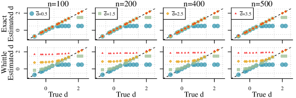
Figure 3: Average estimates of $d$ across 10,000 ARFIMA$\left(0,d,0\right)$ time series with $\mu=0$ and $\sigma^{2}=1$ from maximizing exact or Whittle likelihoods with respect to $d$, $\mu$, and $\sigma^{2}$.

The first row of Figure 3 shows the average estimates of $d$ obtained by maximizing the exact likelihood with respect to $d$, $\mu$, and $\sigma^{2}$. We consider upper bounds $\bar{d}$ that exceed the true data generating value of $d$. We estimate $d$ well at all sample sizes as long as $\bar{d}$ exceeds the true value of $d$. Surprisingly, we estimate $d$ well even when the true value of $d$ is much smaller than $\bar{d}$, e.g., when the true value of $d$ is negative and $\bar{d}>0.5$. This suggests that we do not pay a high price for overdifferencing the data when we are interested in obtaining a point estimate of the memory parameter $d$ by maximizing the exact likelihood.

The second and third rows of Figure 3 show average estimates of $d$ obtained by maximizing the Whittle approximate likelihood with respect to $d$, $\mu$, and $\sigma^{2}$, respectively. Whittle estimates of $d$ are much more sensitive to the choice of $\bar{d}$; they are biased if $\bar{d}$ is too large or too small. Not only do they underestimate the memory parameter $d$ when the true value of the memory parameter exceeds $\bar{d}$, they also systematically overestimate $d$ when $\bar{d}$ exceeds the true value of $d$, especially when $\bar{d}$ is much larger than the true value of $d$. For the approximate likelihood estimator, we pay a price for overdifferencing. The Whittle approximate likelihood based estimators of $d$ performs relatively well only when the true value $d$ satisfies $\bar{d}-1.5\leq d\leq\bar{d}$. The Whittle estimator’s systematic overestimation of $d$ when the true value $d\leq-0.5$ is consistent with the literature. Hurvich and Ray (1995) demonstrated that the log periodogram is biased when the memory parameter $d\leq-0.5$ in such a way that leads to overestimation of the memory parameter, and Hurvich and Chen (2000) observed this phenomenon in simulations.

3.2 Interval Estimation of the Memory Parameter for Fixed $\bar{d}$

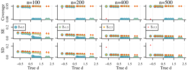
Figure 4: Coverage of 95% confidence intervals for $d$, average standard errors of $\hat{d}$, and standard deviations of $\hat{d}$ across 10,000 ARFIMA$\left(0,d,0\right)$ time series with $\mu=0$ and $\sigma^{2}=1$ from maximizing the exact likelihood with respect to $d$, $\mu$, and $\sigma^{2}$.

In practice, we may also be interested in assessing the uncertainty of our estimate of the memory parameter $d$. Accordingly, for exact likelihood based estimators of the long memory parameter, Figure 4 shows the coverage of 95% confidence intervals for the memory parameter $d$, average standard errors of $\hat{d}$, and approximate standard deviations of $\hat{d}$.

Unsurprisingly, coverage is poor when the true value of the memory parameter $d$ exceeds the maximum value $\bar{d}$. Also unsurprisingly, standard errors are larger and 95% confidence intervals are wider for larger values of $\bar{d}$, especially when $n$ is small. Thus, we pay a small price for overdifferencing when we are interested in assessing the uncertainty of our estimate of the memory parameter $d$ when $\bar{d}$, as long as $\bar{d}$ is not too large. However, we pay a high price for overdifferencing if $\bar{d}$ is especially large relative to the true value of the long memory parameter, specifically if the difference between $\bar{d}$ exceeds the true value of the long memory parameter by three or more, even when $n$ is large. Specifically, we obtain 95% intervals with near zero coverage and standard errors that vastly underestimate the variability of $\hat{d}$. This is caused by numerical instability of the likelihood when $d\in\left(-0.5+m_{\bar{d}}-j,0.5+m_{\bar{d}}-j\right)$ and $j\geq 4$. We evaluate the likelihood in this range by computing the likelihood of a stationary ARFIMA$\left(p,d-m_{\bar{d}}+j,j+q\right)$ model with $j+q$ constrained moving average parameters $\tilde{\theta}_{1}^{\left(j\right)},\dots,\tilde{\theta}^{\left(j\right)}_{j+q}$ obtained by expanding out $\left(1-B\right)^{j}\theta\left(B\right)$. Although this corresponds to the likelihood of a stationary process and thus corresponds to a positive definite variance-covariance matrix of the differenced data, we find that the variance-covariance matrix of the differenced data can become ill-conditioned when $n$ is large, and lead to failure of the adjusted version of Durbin’s algorithm used to evaluate the likelihood. This is explored in detail in Section I of the Online Appendix and is consistent with existing research that finds poor performance of the Durbin-Levinson algorithm for ill-conditioned positive definite Toeplitz matrices (Gohbert et al., 1995).

3.3 Adaptive Point Estimation of the Memory Parameter

The results of the previous section, in particular the second two rows of Figures 3 and 4, motivate the need for the adaptive methods introduced in Section 2.2. We abbreviate the procedure obtained by setting $\epsilon=0.5$ as BND because it checks that the log-likelihood is decreasing in $d$ at the upper boundary $\bar{d}$. We abbreviate procedures obtained by setting $\epsilon<0.5$ as BFR$\left(\epsilon\right)$ because they ensure that a buffer between $\hat{d}$ and the upper boundary $\bar{d}$ by requiring that the approximate $\left(1-\epsilon\right)\times 100\%$ percentile of $d$ be less than the upper boundary $\bar{d}$. We consider three different values of $\epsilon=5\times 10^{-s}$ corresponding to $s\in\left\{2,4,16\right\}$. We note that $s=16$ is the largest integer that returned a finite $\left(1-5\times 10^{-s}\right)\times 100\%$ standard normal percentile, given the version of R we were using. The choice $s=16$ requires that $\hat{d}$ be at least $8.014$ standard errors from the boundary $\bar{d}$. While this may seem extreme, it may be appropriate given that the standard error is an estimate of the standard deviation of the sampling distribution of $\hat{d}$ and given that a normal distribution may be a poor approximation of the sampling distribution of $\hat{d}$ in finite samples. Figure 5 shows average estimates of $d$ obtained using the BND and BFR$\left(\epsilon\right)$ exact and the BND Whittle procedures. The BND procedure and all three BFR$\left(\epsilon\right)$ exact procedures estimate $d$ well, regardless of the value of $\epsilon$ chosen or true value of the memory parameter. The BND Whittle procedure produces excellent estimates of $d$ regardless of the true value of the memory parameter, especially when $n$ is large.

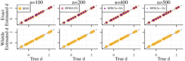
Figure 5: Average BND and BFR$\left(\epsilon\right)$ estimates of $d$ across $10,000$ ARFIMA$\left(0,d,0\right)$ time series with $\mu=0$ and $\sigma^{2}=1$ for different values of $\epsilon$, which determines the percentile used to choose $\bar{d}$. When estimating $d$, the $\mu$ and $\sigma^{2}$ are treated as unknown.

3.4 Adaptive Interval Estimation of the Memory Parameter

In our final simulation study, we examine the coverage of BND and BFR$\left(\epsilon\right)$ $95\%$ confidence intervals for $d$ obtained from the exact likelihood maximizing estimates. Figure 3.4 shows that the best coverage rates were obtained by setting $\epsilon=5\times 10^{-16}$. This suggests the simple strategy of choosing the smallest possible $\epsilon$. The BND and BFR$\left(\epsilon\right)$ $95\%$ confidence intervals generally behave as we would hope; they produce interval estimates whose coverage converges to $0.95$ as $n$ increases. Additionally, the performance of BFR$\left(\epsilon\right)$ $95\%$ confidence intervals does not seem very sensitive to the choice of $\epsilon$, especially when $n$ is large.

The greatest gains of BFR$\left(\epsilon\right)$ over BND confidence intervals are obtained when the true memory parameter $d$ is near boundary values $0.5,1.5,2.5$ and $n$ is small. The BND procedure can yield estimates $\hat{d}_{\bar{d}}$ that are very close to the boundary $\bar{d}$, where the asymptotic normal approximations to the sampling distribution of $\hat{d}_{\bar{d}}$ used to construct approximate confidence intervals are known to be poor. In contrast, the BFR$\left(\epsilon\right)$ procedure is more likely to yield estimates $\hat{d}_{\bar{d}}$ that are far from the boundary $\bar{d}$. The same patterns are observed when comparing BFR$\left(\epsilon\right)$ intervals computed using smaller versus larger values of $\epsilon$.

3.5 Comparison to Alternatives

We compare the absolute bias of the adaptive exact and Whittle likelihood estimators of $d$ to the absolute bias of two alternatives, one which treats the mean $\mu$ and variance $\sigma^{2}$ as unknown and one which treats the mean $\mu$ as known and equal to its true value and treats $\sigma^{2}$ as unknown. Specifically, we compare to a CSS approximate likelihood estimator as described in Beran (1995), Hualde and Robinson (2011), and Hualde and Nielsen (2020) which treats the mean $\mu$ and variance $\sigma^{2}$ as unknown, and we compare to the most favorable oracle implementation of the generalized minimum distance (GMD) estimator introduced by Mayoral (2007), which treats the mean $\mu$ as known and equal to its true value and treats $\sigma^{2}$ as unknown. The GMD estimator requires specification of the number of sample autocorrelations to include in the objective function, denoted by $k$. We consider the most favorable oracle implementation of the GMD estimator which we call “Best GMD” by using the the number of sample autocorrelations $k$ that yields the least biased GMD estimator for each value of the true $d$ and sample size $n$. We do not consider the estimator introduced by Velasco and Robinson (2000) because simulation results from Mayoral (2007) show that it is more biased and variable than the GMD estimator for these simulation settings. Figure 6 shows the average absolute bias of the BND exact estimator, the BFR$\left(5\times 10^{-16}\right)$ exact estimator and the BND Whittle estimator compared to the average absolute bias of the CSS estimator and the Best GMD estimator. Average absolute bias for the Best GMD estimator is reprinted from Mayoral (2007). As in this paper, Mayoral (2007) simulates ARFIMA$\left(p,d,q\right)$ time series with mean $0$ and error variance $\sigma^{2}=1$, but performs 5,000 simulations for each pair of memory parameter $d$ and sample size $n$ values.

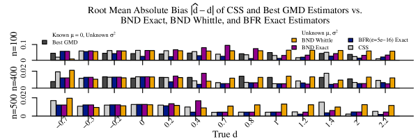
Figure 6: Root average absolute bias of CSS, BND, and BFR$\left(5\times 10^{-16}\right)$ estimators and the Best GMD estimator of $d$ across 100 and 5,000 ARFIMA$\left(0,d,0\right)$ time series with mean $\mu=0$ and variance $\sigma^{2}=1$, respectively, reprinted from Mayoral (2007) for Best GMD. For the CSS, BND, and BFR$\left(5\times 10^{-16}\right)$ estimators, we assume $\mu_{t}=\mu$ and treat $\mu$ and $\sigma^{2}$ as unknown.

Figure 6 shows that our adaptive exact estimators, especially the BFR$\left(5\times 10^{-16}\right)$ estimator, are less biased in many settings. Our adaptive Whittle likelihood estimator is the most biased estimator when $d\geq 0.5$. In comparison to the Best GMD estimator, the BFR$\left(5\times 10^{-16}\right)$ performs better when $d\geq 0$ regardless of the sample size. As the sample size increases, the BND exact estimator outperforms the Best GMD estimator for all $d\geq 0$. This is noteworthy given that the BFR$\left(\epsilon\right)$ estimator summarized in Figure 6 treats the overall mean $\mu$ and variance $\sigma^{2}$ as unknown, whereas the Best GMD estimator treats the overall mean $\mu$ as constant and known to be equal to $0$ and the variance $\sigma^{2}$ as unknown.

Comparison to the CSS estimator suggests systematically poorer performance of the CSS estimator versus most adaptive estimators when the true value of $d$ is close to the boundaries of stationarity, $0.5$, and $1.5$, even as the sample size increases. When the sample size is smaller, the BFR$\left(5\times 10^{-16}\right)$ estimator performs better than the CSS estimator when $-0.3\leq d\leq 1.4$, the BND exact estimator performs better than the CSS estimator when $d\in\left\{-0.2,0,1.4\right\}$. As the sample size increases, the BFR$\left(5\times 10^{-16}\right)$ estimator outperforms the CSS estimator when $d\in\left\{-0.7,0,0.2,0.4,1.4\right\}$, the BND exact estimator outperforms the CSS estimator when $d\in\left\{-0.7,0,1.4\right\}$. We also find that the variability of our adaptive estimators is comparable to the variability of the CSS estimator and the Best GMD estimator for most sample sizes and true values of $d$. Additionally, we find that our adaptive estimators of the noise variance $\sigma^{2}$, especially the BND exact and BFR$\left(5\times 10^{-16}\right)$ exact estimators of $\sigma^{2}$, tend to be less biased than the CSS estimator of $\sigma^{2}$ in the presence of long memory, even as the sample size increases. More details regarding variability of estimators and estimation of the noise variance are provided in Sections C and D of the Online Appendix. We did not explore estimation of the overall mean $\mu$ because, like other estimators of based on integer differenced data, the BND and BFR$\left(\epsilon\right)$ estimators of $\mu$ are not unique after differencing. In additional simulations summarized in Sections E-G of the Online Appendix, we find that the relative performances of the proposed estimators to each other and alternatives persist when the mean is assumed to be a quadratic time trend that is not cancelled by pre-differencing when $\bar{d}\leq 3.5$, and when observations are non-Gaussian.

4 Applications

4.1 Chemical Process Concentration and Temperature

Because Beran (1995) considered the same problem as this paper, we begin by applying our methods to fit ARFIMA$\left(0,d,0\right)$ models with $\mu_{t}=\mu$ to the examples discussed in Beran (1995): the chemical process concentration readings (Series A) and the chemical process temperature readings (Series C). Descriptive plots of Series A and Series C are provided in Section J of the Online Appendix. For both, we consider exact likelihood estimation of the memory parameter because we are interested in obtaining point and interval estimates. Based on the results of the simulation study which suggest that choosing the smallest possible $\epsilon$ yields the best performance, we compute BFR$\left(\epsilon=5\times 10^{-16}\right)$ exact likelihood estimates. Analogous results for the Whittle and SCSS approximate likelihoods and corresponding BND estimates are provided in Section J of the Online Appendix.

Table 1, which shows the exact estimates of $d$ for $\bar{d}\in\left\{0.5,1.5,2.5\right\}$, with the BFR$\left(\epsilon\right)$ exact likelihood estimates highlighted in gray. Exact profile log-likelihood curves for $\bar{d}\in\left\{0.5,1.5,2.5\right\}$, with $\mu$ and $\sigma^{2}$ profiled out are provided in Section J of the Online Appendix. We observe that the exact likelihood curves retain the same shape as $\bar{d}$ increases; both the maximizing value of $d$ and the curvature about the maximizing value change little as $\bar{d}$ increases. When computing estimates using the BFR$\left(\epsilon\right)$ procedure, we set $\epsilon=5\times 10^{-16}$ based on the simulation results discussed in Section 3.4.

Series	$n$	$\bar{d}$	$\hat{d}_{\bar{d}}$	95% Interval for $d$	Series	$n$	$\bar{d}$	$\hat{d}_{\bar{d}}$	95% Interval for $d$
A	$197$	$0.5$	$0.400$	$\left(0.304,0.496\right)$	C	$226$	$0.5$	$0.500$	$-$
		$1.5$	$0.427$	$\left(0.319,0.534\right)$			$1.5$	$1.500$	$-$
		$2.5$	$0.436$	$\left(0.326,0.545\right)$			$2.5$	$1.788$	$\left(1.659,1.918\right)$

Table 1: Estimates and intervals for $d$ for Series A and C, treating $\mu$ and $\sigma^{2}$ are treated as unknown. BFR$\left(\epsilon=5\times 10^{-16}\right)$ estimates given in gray. Intervals provided when the log-likelihood is decreasing at $\bar{d}$.

From Table 1, we see that the choice of $\bar{d}$ affects the exact likelihood estimates of $d$ minimally and the 95% intervals for the exact likelihood estimates of $d$ substantively. The 95% intervals for $\bar{d}=1.5$, the BFR$\left(\epsilon=5\times 10^{-16}\right)$ exact likelihood estimate of $d$, and $\bar{d}=2.5$, for the Series A data contain $0.5$, which suggests that the Series A data may not be stationary. This is consistent with Beran (1995), which used an approximate likelihood method to obtain an estimate $\hat{d}=0.41$ and a 95% confidence interval of $\left(0.301,0.519\right)$.

As in Beran (1995), we also fit ARFIMA$\left(0,d,1\right)$ and ARFIMA$\left(1,d,0\right)$ models with $\mu_{t}=\mu$ to the Series A and C data, respectively, for different values of $\bar{d}$. ARFIMA$\left(p,d,q\right)$ models are more computationally challenging to fit than ARFIMA$\left(0,d,0\right)$ models because evaluating the likelihood is much computationally intensive and the likelihood can have many modes. Table 2 shows the corresponding parameter estimates we obtain for both data sets for $\bar{d}\in\left\{0.5,1.5,2.5,3.5\right\}$, with the BFR$\left(\epsilon=5\times 10^{-16}\right)$ exact likelihood estimates highlighted in gray. Examining the estimates of an ARFIMA$\left(0,d,1\right)$ model for Series A, we observe striking changes in the exact likelihood estimates of $d$ and $\theta_{1}$ as $\bar{d}$ changes, and substantial differences between several of the exact and approximate maximum likelihood estimates. Furthermore, the 95% intervals corresponding to the BFR$\left(\epsilon=5\times 10^{-16}\right)$ exact estimates for $d$ and $\theta_{1}$ shown in Table 2 do not contain the exact likelihood estimates for $\bar{d}>1.5$. At the same time, the BFR$\left(\epsilon=5\times 10^{-16}\right)$ exact estimates for $d$ and $\theta_{1}$ align well with the estimates $\hat{d}=0.445$, $\hat{\theta}_{1}=-0.056$ and corresponding 95% intervals $\left(0.261,0.629\right)$ and $\left(-0.290,0.179\right)$ found in Beran (1995). This warrants more careful investigation.

		Estimate			95% Interval
Series	$\bar{d}$	$d$	$\theta_{1}$	$\phi_{1}$	$d$	$\theta_{1}$	$\phi_{1}$
A	$0.5$	$0.419$	$-0.037$	$-$	$\left(0.286,0.553\right)$	$\left(-0.227,0.152\right)$	$-$
	$1.5$	$0.502$	$-0.117$	$-$	$\left(0.298,0.707\right)$	$\left(-0.367,0.134\right)$	$-$
	$2.5$	$1.314$	$-0.923$	$-$	$\left(1.138,1.490\right)$	$\left(-1.014,-0.833\right)$	$-$
	$3.5$	$1.310$	$-0.911$	$-$	$\left(1.125,1.495\right)$	$\left(-1.014,-0.809\right)$	$-$
C	$0.5$	$0.500$	$-$	$1.000$	$-$	$-$	$-$
	$1.5$	$0.950$	$-$	$0.850$	$\left(0.693,1.208\right)$	$-$	$\left(0.682,1.019\right)$
	$2.5$	$0.972$	$-$	$0.842$	$\left(0.703,1.241\right)$	$-$	$\left(0.662,1.023\right)$
	$3.5$	$0.971$	$-$	$0.852$	$\left(0.830,1.113\right)$	$-$	$\left(0.757,0.946\right)$

Table 2: Estimates and intervals for ARFIMA$\left(0,d,1\right)$ and ARFIMA$\left(1,d,0\right)$ models with $\mu_{t}=\mu$ for Series A and C, respectively, treating $\mu$ and $\sigma^{2}$ as unknown. BFR$\left(\epsilon=5\times 10^{-16}\right)$ estimates given in gray. Intervals provided when the log-likelihood is decreasing at $\bar{d}$.

			95% Interval
Data	$n$	$\bar{d}$	$d$	$\theta_{1}$	$\phi_{1}$
Series A	$197$	0.5	$\left(0.286,0.553\right)$	$\left(-0.227,0.152\right)$	$-$
		$1.5$	$\left(0.298,0.707\right)$	$\left(-0.367,0.134\right)$	$-$
		$2.5$	$\left(1.138,1.490\right)$	$\left(-1.014,-0.833\right)$	$-$
		$3.5$	$\left(1.125,1.495\right)$	$\left(-1.014,-0.809\right)$	$-$
Series C	$226$	$0.5$	$-$	$-$	$-$
		$1.5$	$\left(0.693,1.208\right)$	$-$	$\left(0.682,1.019\right)$
		$2.5$	$\left(0.703,1.241\right)$	$-$	$\left(0.662,1.023\right)$
		$3.5$	$\left(0.830,1.113\right)$	$-$	$\left(0.757,0.946\right)$

Table 3: 95% intervals for exact likelihood estimates of the parameters of ARFIMA$\left(0,d,1\right)$ and ARFIMA$\left(1,d,0\right)$ processes both with $\mu_{t}=\mu$ fit to the chemical process concentration readings (Series A) and chemical process temperature readings (Series C) for different values of $\bar{d}$. The BFR$\left(\epsilon=5\times 10^{-16}\right)$ exact likelihood estimates are highlighted in gray. 95% intervals for $d$ are provided for values of $\bar{d}$ that correspond to log-likelihoods that are decreasing at $\bar{d}$.

The first row of Figure 7 shows the exact joint log-likelihoods for the Series A data as a function of the moving average parameter $\theta_{1}$ and $d$ for $\bar{d}\in\left\{0.5,1.5,2.5,3.5\right\}$. The exact log-likelihood is multimodal when $\bar{d}>0.5$, one with $d<1$ and another with $d>1$. Which mode maximizes the likelihood depends on the choice of $\bar{d}$; the maximum likelihood estimates for $\bar{d}\leq 1.5$ corresponds to the mode with $d<1$, whereas the maximum likelihood estimate for $\bar{d}>1.5$ corresponds to the mode with $d>1$. This suggests possibly poor identifiability of the parameters of the ARIMA$\left(p,d,q\right)$ model even in simple cases with $p=0$ and $q=1$, which should be considered whenever an ARIMA$\left(p,d,q\right)$ is applied.

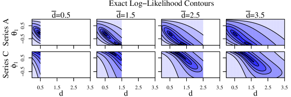
Figure 7: Exact profile log-likelihoods for ARFIMA$\left(0,d,1\right)$ and ARFIMA$\left(1,d,0\right)$ models with $\mu_{t}=\mu$ for Series A and Series C data, respectively, with $\mu$ and $\sigma^{2}$ profiled out.

We revisit Table 2 to examine estimates of the parameters of an ARFIMA$\left(1,d,0\right)$ model for Series C and see more stable estimates across values of $\bar{d}$. The BFR$\left(\epsilon=5\times 10^{-16}\right)$ exact likelihood estimates of $\hat{d}_{\bar{d}}=0.972$ and $\hat{\phi}_{\bar{d},1}=0.842$, with corresponding 95% intervals of $\left(0.684,1.261\right)$ and $\left(0.654,1.031\right)$ are consistent with the approximate likelihood estimates $\hat{d}=0.905$ and $\hat{\phi}_{1}=0.864$ and 95% confidence intervals $\left(0.662,1.148\right)$ and $\left(0.708,1.00\right)$ provided in Beran (1995). We do not observe evidence of multimodality of the exact log-likelihoods in Table 2, however the joint log-likelihoods in the second row of Figure 7 are banana shaped near the maximum. Again, this reflects somewhat poor identifiability of $d$ and $\phi_{1}$ and further emphasizes the need for care when applying ARIMA$\left(p,d,q\right)$ models.

4.2 $\text{CO}_{2}$ Emissions

Barassi et al. (2018) uses long memory models to assess whether relative per capita CO₂ emissions of 28 OECD countries are consistent with mean reverting long memory processes that may converge to a linear trend over enough time. Letting $y_{tc}$ be the relative per capita CO₂ emissions of country $c$ at time $t$ as defined in Barassi et al. (2018), they assume that deviations of the relative per capita CO₂ emissions of each country $y_{tc}$ from an overall mean and country-specific linear trend $\mu_{tc}=\mu_{c}+\beta_{c}t$ are distributed according to an ARFIMA$\left(0,d_{c},0\right)$ process, with $\left(1-B\right)^{d_{c}}\left(y_{tc}-\mu_{c}-\beta_{c}t\right)=z_{tc}$, $z_{tc}\stackrel{{\scriptstyle i.i.d.}}{{\sim}}\mathcal{N}\left(0,\sigma^{2}_{c}\right)$, and error variances $\sigma^{2}_{c}$. Under this model, country $c$’s relative per capita CO₂ emissions are mean reverting if $d_{c}<1$. Accordingly, they assess whether each country’s relative per capita CO₂ emissions are mean reverting by testing the null hypothesis $d_{c}\geq 1$ for each country.

Treating the country-specific means $\mu_{c}$, slopes $\beta_{c}$, and variances $\sigma^{2}_{c}$ as unknown, we perform level $\alpha=0.05$ tests of the null hypotheses that $d_{c}\geq 1$ versus the alternative that $d_{c}<1$ for each country by comparing the upper bound of the 90% confidence interval for the BFR$\left(\epsilon=5\times 10^{-16}\right)$ exact likelihood estimate $\hat{d}_{c}$ to $1$ and rejecting if it fails to exceed $1$. Figure 8 shows the 90% confidence intervals for the BFR$\left(\epsilon=5\times 10^{-16}\right)$ exact likelihood estimates for all 28 OECD countries. We reject the null hypothesis that $d_{c}\geq 1$ for Iceland, Austria, Denmark, Ireland, Switzerland, Norway, and the Netherlands. This is largely consistent with Barassi et al. (2018), which reports strong evidence of mean reversion for Austria, Denmark, Finland, Iceland, Ireland, Israel, Norway and Switzerland based on a battery of alternative methods, many of which depend on the choice of several tuning parameters. One apparent disagreement between our findings and those of Barassi et al. (2018) is that Barassi et al. (2018) conclude that there is strong evidence that Israel’s per capita CO₂ emissions are mean reverting, whereas we are not able to estimate the memory parameter for Israel with enough precision to reject the null hypothesis that $d_{c}\geq 1$.

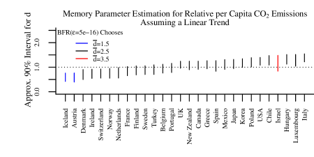
Figure 8: 90% intervals for BFR$\left(\epsilon=5\times 10^{-16}\right)$ exact likelihood estimates of $d$.

4.3 ECIS Measurements

Last, we compute BFR$\left(\epsilon=5\times 10^{-16}\right)$ exact likelihood estimates of the memory parameter for several observed time series of ECIS measurements, which is a relatively new tool for monitoring the growth and behavior of cells in culture (Giaever and Keese, 1991). Previous research has suggested that ARFIMA$\left(0,d,0\right)$ models may be appropriate for ECIS measurements, and it has been hypothesized that the memory parameter $d$ may vary by cell type and contamination status (Giaever and Keese, 1991; Tarantola et al., 2010; Gelsinger et al., 2020; Zhang et al., 2020). We consider ECIS measurements from eight experiments, four conducted using Madin-Darby canine kidney (MDCK) cells and African green monkey kidney epithelial (BSC-1) cells. From each experiment, we examine 40 individual time series of about $n\approx 170$ measurements, which correspond to measurements from 40 cell filled wells on a single tray collected between 40 and 72 hours after the wells were filled and the experiment began. Of the 40 wells examined in each experiment, half were prepared using one medium referred to as BSA and half were prepared using another medium referred to as gel. Of the 20 wells in each experiment prepared with the same medium, 12 contain cells contaminated by mycoplasma and 8 contain uncontaminated cells. Letting $y_{temwf}$ refer to ECIS measurements for well $w$ prepared with medium $m$ in experiment $e$ measured at frequency $f$, we assume that the mean $\mu_{temwf}=\mu_{emwf}$ is constant over time and

$$\begin{array}[]{ll}\left(1-B\right)^{d_{emf}^{\left(1\right)}}\left(y_{temwf}-\mu_{emwf}\right)=z_{temwf}&\text{ for wells $w$ with contaminated cells and}\\ \left(1-B\right)^{d_{emf}^{\left(0\right)}}\left(y_{temwf}-\mu_{emwf}\right)=z_{temwf}&\text{ otherwise,}\end{array}$$

where $z_{temwf}\stackrel{{\scriptstyle i.i.d.}}{{\sim}}\mathcal{N}\left(0,\sigma^{2}_{emwf}\right)$. Pooling over ECIS measurements with the same cells, contamination status, and preparation in the same experiment, we obtain pairs of estimates of the memory parameters $d^{\left(0\right)}_{emf}$ and $d^{\left(1\right)}_{emf}$ for each experiment, medium, and frequency.

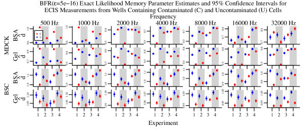
Figure 9: BFR$\left(\epsilon=5\times 10^{-16}\right)$ exact likelihood estimates and 95% intervals for memory parameters $d^{\left(0\right)}_{emf}$ (blue) and $d^{\left(1\right)}_{emf}$ (red). When estimating $d^{\left(0\right)}_{emf}$ and $d^{\left(1\right)}_{emf}$, $\mu_{emwf}$ and $\sigma^{2}_{emwf}$ are treated as unknown.

Figure 9 shows some evidence that ECIS measurements may have long memory behavior that depends on contamination status. We see longer memory in measurements of contaminated MDCK cells prepared using BSA at 32,000 Hz, shorter memory in measurements of contaminated MDCK cells prepared using gel at 4,000 and 8,000 Hz, shorter memory in measurements of contaminated BSC-1 cells prepared using BSA at 32,000 Hz, and shorter memory in measurements of contaminated BSC-1 cells prepared using gel at all frequencies, especially 32,000 Hz. This preliminary analysis suggests that long memory behavior of ECIS measurements may help distinguish contaminated from uncontaminated cells, although the sample sizes are small and the scope is limited.

5 Conclusion

In this paper, we make a simple but powerful observation that allows us to perform exact likelihood estimation of the parameters of ARFIMA$\left(p,d,q\right)$ models without restricting the memory parameter $d$ to the range of values that correspond to a stationary ARFIMA$\left(p,d,q\right)$ process. We introduce adaptive procedures for specifying an upper bound for the memory parameter that allow for parsimonious inference. We demonstrate the utility of this method via simulation studies and applications, both to canonical datasets that have been explored in the ARFIMA$\left(p,d,q\right)$ literature and to more modern datasets. We emphasize that this allows us to compare exact and approximate likelihood methods and identify both situations where approximate likelihood methods perform well and where they have shortcomings relative to exact likelihood methods.

There are many future directions to pursue. Alternative likelihood approximations may provide better estimates of the memory parameter. In particular, we observe that Whittle estimates tend to be biased, which is a well known limitation of Whittle likelihood estimates (Contreras-Cristán et al., 2006). Using one of the novel approximations introduced in Jesus and Chandler (2017), Sykulski et al. (2019), or Das and Yang (2020) in place of the Whittle likelihood may yield less biased approximate estimators. Second, incorporating approximate sampling distributions for Whittle estimators, e.g. those described in Velasco and Robinson (2000), may yield BFR$\left(\epsilon\right)$ Whittle estimators that outperform the BND Whittle estimators considered here. Third, alternative approaches to approximating standard errors and confidence intervals may provide better standard error and interval estimates. We have used numerical differentiation throughout this paper to approximate standard errors and confidence intervals. As shown in Section J of the Online Appendix, confidence intervals corresponding to BND and BFR$\left(\epsilon\right)$ exact likelihood estimators perform well on average across the simulations considered in this paper, however they can be unstable in individual simulations. Fortunately, the methods we introduce in this paper ease the use of modern techniques, e.g. the parametric bootstrap, for approximating the sampling distribution of the memory parameter $d$ by ensuring that the estimate $d$ is far from the upper boundary $\bar{d}$. Fourth, replacing the adjusted version of Durbin’s algorithm used to evaluate the likelihood with an alternative algorithm that is more suitable for ill conditioned covariance matrices, e.g. the algorithm described in (Gohbert et al., 1995), may improve performance of the exact likelihood estimator for large maximum values $\bar{d}$ when the true value of the memory parameter $d$ is much smaller than $\bar{d}$, thus reducing the need for an adaptive approach altogether. Fifth, the performance of our proposed estimators for non-Gaussian processes in simulations suggests the value of extending the consistency and asymptotic normality results provided in (Lieberman et al., 2012) to non-Gaussian processes. Sixth, simulation studies investigating the finite sample properties of our proposed estimators when $p+q>0$ would be valuable for assessing the relative merits of the proposed approach compared to alternatives. Last, this approach may provide a useful framework for obtaining exact likelihood estimation for multivariate fractional differencing models, which may provide performance advantages in comparison to existing approximate methods such as the CSS approximate likelihood estimator introduced in Nielsen (2015).

SUPPLEMENTARY MATERIAL

A stand-alone package for implementing the methods described in this paper can be downloaded from https://github.com/maryclare/nslm.

Appendix A Continuity of $l_{\bar{d}}\left(\boldsymbol{x}^{\left(m_{\bar{d}}\right)}|d,\mu_{t},\sigma,\boldsymbol{\theta},\boldsymbol{\phi}\right)$

Theorem A.1

The log-likelihood $l_{\bar{d}}\left(\boldsymbol{x}^{\left(m_{\bar{d}}\right)}|d,\mu_{t},\sigma,\boldsymbol{\theta},\boldsymbol{\phi}\right)$ is continuous for $-0.5+m_{\bar{d}}-k\leq d<\bar{d}$.

• Continuity of $l_{\bar{d}}\left(\boldsymbol{x}^{\left(m_{\bar{d}}\right)}|d,\mu_{t},\sigma,\boldsymbol{\theta},\boldsymbol{\phi}\right)$ on the intervals $\left[-0.5+m_{\bar{d}}-j,0.5+m_{\bar{d}}-j\right)$ for $j=0,\dots,k$ follows from continuity of the log-likelihood of a stationary ARFIMA$\left(p,d,q\right)$ process (Dahlhaus, 1989). Note that Dahlhaus (1989) requires stationarity of the ARFIMA$\left(p,d,q\right)$ but does not require that roots of the moving average polynomial $\theta\left(x\right)$ lie strictly outside the unit circle.

  Continuity of $l_{\bar{d}}\left(\boldsymbol{x}^{\left(m_{\bar{d}}\right)}|d,\mu_{t},\sigma,\boldsymbol{\theta},\boldsymbol{\phi}\right)$ at $d=-0.5+m_{\bar{d}}-j$ for $j=0,\dots,k-1$ requires

  $$\text{lim}_{\varepsilon\rightarrow 0^{+}}l_{\bar{d}}\left(\boldsymbol{x}^{\left(m_{\bar{d}}\right)}|0.5+m_{\bar{d}}-\left(j+1\right)-\varepsilon,\mu_{t},\sigma,\boldsymbol{\theta},\boldsymbol{\phi}\right)=$$

  $$\quad\quad\quad\quad\quad\quad l_{\bar{d}}\left(\boldsymbol{x}^{\left(m_{\bar{d}}\right)}|-0.5+m_{\bar{d}}-j,\mu_{t},\sigma,\boldsymbol{\theta},\boldsymbol{\phi}\right).$$

  Let $\boldsymbol{\Omega}\left(d,\boldsymbol{\theta},\boldsymbol{\phi},\sigma\right)$ refer to the $\left(n-m_{\bar{d}}\right)\times\left(n-m_{\bar{d}}\right)$ covariance matrix of the stationary differenced data $\boldsymbol{x}^{\left(m_{\bar{d}}\right)}$ with elements $\omega\left(d,\boldsymbol{\theta},\boldsymbol{\phi},\sigma\right)_{ii^{\prime}}$ given by the autocovariance function $\omega\left(\left|i-i^{\prime}\right|;d,\boldsymbol{\theta},\boldsymbol{\phi},\sigma\right)$. The log-likelihood $l_{\bar{d}}\left(\boldsymbol{x}^{\left(m_{\bar{d}}\right)}|d,\mu_{t},\sigma,\boldsymbol{\theta},\boldsymbol{\phi}\right)$ is

  $$l_{\bar{d}}\left(\boldsymbol{x}^{\left(m_{\bar{d}}\right)}|d,\mu,\sigma,\boldsymbol{\theta},\boldsymbol{\phi}\right)=- n\text{log}\left(2\pi\right)/2-\text{log}\left(\left|\boldsymbol{\Omega}\left(d,\boldsymbol{\theta},\boldsymbol{\phi},\sigma\right)\right|\right)/2-$$

  $$\left(\boldsymbol{x}^{\left(m_{\bar{d}}\right)}-\boldsymbol{\mu}^{\left(m_{\bar{d}}\right)}\right)^{\prime}\boldsymbol{\Omega}\left(d,\boldsymbol{\theta},\boldsymbol{\phi},\sigma\right)^{-1}\left(\boldsymbol{x}^{\left(m_{\bar{d}}\right)}-\boldsymbol{\mu}^{\left(m_{\bar{d}}\right)}\right)/2.$$

  Because the log-likelihood depends on $d$ only through the autocovariance function and is a continuous function of the autocovariance function, the log-likelihood $l_{\bar{d}}\left(\boldsymbol{x}^{\left(m_{\bar{d}}\right)}|d,\mu_{t},\sigma,\boldsymbol{\theta},\boldsymbol{\phi}\right)$ is continuous at $d=-0.5+m_{\bar{d}}-j$ if the autocovariance function is continuous at $d=-0.5+m_{\bar{d}}-j$,

  $$\text{lim}_{\varepsilon\rightarrow 0^{+}}\omega\left(h;0.5+m_{\bar{d}}-\left(j+1\right)-\varepsilon,\boldsymbol{\theta},\boldsymbol{\phi},\sigma\right)=\omega\left(h;-0.5+m_{\bar{d}}-j,\boldsymbol{\theta},\boldsymbol{\phi},\sigma\right).$$

  Letting $\gamma\left(h;d,\boldsymbol{\theta},\boldsymbol{\phi},\sigma\right)$ refer to the autocovariance function of a mean-zero stationary ARFIMA$\left(p,d,q\right)$ process with parameters $d$, $\boldsymbol{\theta}$, $\boldsymbol{\phi}$, and $\sigma^{2}$, and letting $\tilde{\boldsymbol{\theta}}^{(j)}$ refer to the coefficients of the moving average polynomial $\left(1-B\right)^{j}\theta\left(B\right)$, we have

  $$\text{lim}_{\varepsilon\rightarrow 0^{+}} \omega\left(h;0.5+m_{\bar{d}}-\left(j+1\right)-\varepsilon,\boldsymbol{\theta},\boldsymbol{\phi},\sigma\right)=\text{lim}_{\varepsilon\rightarrow 0^{+}}\gamma\left(h;0.5-\varepsilon,\tilde{\boldsymbol{\theta}}^{\left(j+1\right)},\boldsymbol{\phi},\sigma\right)=$$

  $$\text{lim}_{\varepsilon\rightarrow 0^{+}}\int_{-\pi}^{\pi}\text{exp}\left\{ih\nu\right\}\left(\frac{\sigma^{2}\left|\tilde{\theta}^{\left(j+1\right)}\left(\text{exp}\left\{-i\nu\right\}\right)\right|^{2}}{2\pi\left|\phi\left(\text{exp}\left\{-i\nu\right\}\right)\right|^{2}}\right)\left|1-\text{exp}\left\{-i\nu\right\}\right|^{-2\left(0.5-\varepsilon\right)}d\nu=$$

  $$\text{lim}_{\varepsilon\rightarrow 0^{+}}\int_{-\pi}^{\pi}\text{exp}\left\{ih\nu\right\}\left(\frac{\sigma^{2}\left|\left(1-\text{exp}\left\{-i\nu\right\}\right)^{j+1}\theta\left(\text{exp}\left\{-i\nu\right\}\right)\right|^{2}}{2\pi\left|\phi\left(\text{exp}\left\{-i\nu\right\}\right)\right|^{2}}\right)\left|1-\text{exp}\left\{-i\nu\right\}\right|^{-2\left(0.5-\varepsilon\right)}d\nu=$$

  $$\text{lim}_{\varepsilon\rightarrow 0^{+}}\int_{-\pi}^{\pi}\text{exp}\left\{ih\nu\right\}\left(\frac{\sigma^{2}\left|\left(1-\text{exp}\left\{-i\nu\right\}\right)^{j}\theta\left(\text{exp}\left\{-i\nu\right\}\right)\right|^{2}}{2\pi\left|\phi\left(\text{exp}\left\{-i\nu\right\}\right)\right|^{2}}\right)\left|1-\text{exp}\left\{-i\nu\right\}\right|^{-2\left(0.5-\varepsilon-1\right)}d\nu=$$

  $$\text{lim}_{\varepsilon\rightarrow 0^{+}}\int_{-\pi}^{\pi}\text{exp}\left\{ih\nu\right\}\left(\frac{\sigma^{2}\left|\tilde{\theta}^{(j)}\left(\text{exp}\left\{-i\nu\right\}\right)\right|^{2}}{2\pi\left|\phi\left(\text{exp}\left\{-i\nu\right\}\right)\right|^{2}}\right)\left|1-\text{exp}\left\{-i\nu\right\}\right|^{-2\left(-0.5-\varepsilon\right)}d\nu=$$

  $$\text{lim}_{\varepsilon\rightarrow 0^{+}}\gamma\left(h;-0.5-\varepsilon,\tilde{\boldsymbol{\theta}}^{\left(j\right)},\boldsymbol{\phi},\sigma\right)=\gamma\left(h;-0.5,\tilde{\boldsymbol{\theta}}^{\left(j\right)},\boldsymbol{\phi},\sigma\right)=\omega\left(h;-0.5+m_{\bar{d}}-j,\boldsymbol{\theta},\boldsymbol{\phi},\sigma\right).$$

  Throughout, we make use of derivations of the spectral density and autocovariance function of an ARFIMA$\left(p,d,q\right)$ process in Sowell (1992). Although Sowell (1992) focuses on stationary ARFIMA$\left(p,d,q\right)$ process with roots of the autoregressive and moving average polynomials $\phi\left(x\right)$ and $\theta\left(x\right)$ outside the unit circle and $-0.5<d<0.5$, the derivations themselves do not require that the roots of the moving average polynomial $\theta\left(x\right)$ lie strictly outside the unit circle and allow for $-1<d\leq-0.5$.

Appendix B The SCSS Approximate Likelihood

The SCSS approximation is obtained by assuming that the finite differences

$$\left(1-B\right)_{+}^{d-m_{\bar{d}}+j}(x^{\left(m_{\bar{d}}\right)}_{t}-\mu^{\left(m_{\bar{d}}\right)}_{t})$$

are distributed according to an ARFIMA$\left(p,0,j+q\right)$ process. The SCSS likelihood is not continuous. The SCSS likelihood is not generally equivalent to the CSS likelihood, which assumes that the finite differences $\left(1-B\right)_{+}^{d}\left(y_{t}-\mu_{t}\right)$ are distributed according to an ARFIMA$\left(p,0,q\right)$ process. The second and third rows of Figure 10 show average estimates of $d$ obtained by maximizing the Whittle and SCSS approximate likelihoods with respect to $d$, $\mu$, and $\sigma^{2}$, respectively. For the SCSS estimator, we pay a price for overdifferencing. The SCSS approximate likelihood based estimators of $d$ performs relatively well only when the true value $d$ satisfies $\bar{d}-1.5\leq d\leq\bar{d}$.

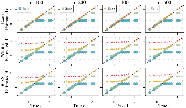
Figure 10: Average estimates of $d$ across 10,000 ARFIMA$\left(0,d,0\right)$ time series with $\mu=0$ and $\sigma^{2}=1$ from maximizing exact Whittle, or SCSS likelihoods with respect to $d$, $\mu$, and $\sigma^{2}$.

At first glance, the SCSS estimator’s tendency to overestimate $d$ when the true value is far less than $\bar{d}$ may appear to conflict with the existing literature, specifically Hualde and Robinson (2011). Hualde and Robinson (2011) demonstrate consistency and asymptotic normality of CSS estimators for arbitrary values of the differencing parameter $d$ when the truncated fractional differences $\left(1-B\right)^{d}_{+}y_{t}$ are distributed according to a stationary ARMA$\left(p,q\right)$ model. However, our results depict the performance of the SCSS estimator when the untruncated fractional differences $\left(1-B\right)^{d}y_{t}$ are distributed according to a stationary ARMA$\left(p,q\right)$ model. The truncated and untruncated models differ, especially when $d\leq-0.5$ and moreso as $d$ decreases below $-0.5$, which corresponds to the case where the true value of the differencing parameter $d$ is far less than the upper bound, specifically $d\leq\bar{d}-1$. The differences between the truncated and untruncated models are illustrated in Section K of the Online Appendix. We believe that this explains how we can observe the systematic overestimation of $d$ by the SCSS estimator shown in Figure 10 while the results of Hualde and Robinson (2011) hold; the results of Hualde and Robinson (2011) hold under a different model for the observed time series data, which diverges more from the model we consider as the true value of $d$ gets further from the upper bound $\bar{d}$.

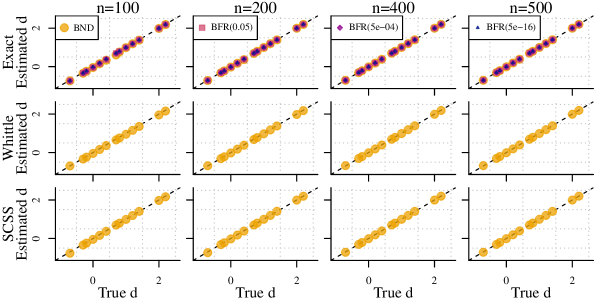
Figure 11: Average BND and BFR$\left(\epsilon\right)$ estimates of $d$ across $10,000$ ARFIMA$\left(0,d,0\right)$ time series with $\mu=0$ and $\sigma^{2}=1$ for different values of $\epsilon$, which determines the percentile used to choose $\bar{d}$. When estimating $d$, the $\mu$ and $\sigma^{2}$ are treated as unknown.

Figure 11 also shows the average estimates of $d$ obtained using the BND Whittle and SCSS procedures, and indicates that the BND SCSS estimator also produces excellent estimates of $d$ regardless of the true value of the memory parameter, especially when $n$ is large.

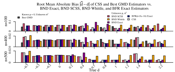
Figure 12: Root average absolute bias of CSS, BND, and BFR$\left(5\times 10^{-16}\right)$ estimators and the Best GMD estimator of $d$ across 100 and 5,000 ARFIMA$\left(0,d,0\right)$ time series with mean $\mu=0$ and variance $\sigma^{2}=1$, respectively, reprinted from Mayoral (2007) for Best GMD. For the CSS, BND, and BFR$\left(5\times 10^{-16}\right)$ estimators, we assume $\mu_{t}=\mu$ and treat $\mu$ and $\sigma^{2}$ as unknown.

We add a comparison of the absolute bias of the BND SCSS estimator to the adaptive exact and Whittle likelihood estimators of $d$ to the absolute bias of two alternatives depicted in Figure 7 of the main manuscript. Figure 12 shows that our adaptive exact and SCSS estimators, especially the BFR$\left(5\times 10^{-16}\right)$ estimator, are less biased in many settings, whereas our adaptive Whittle likelihood estimator is the most biased estimator when $d\geq 0.5$ and performs similarly to our adaptive SCSS estimator otherwise. In comparison to the Best GMD estimator, the BFR$\left(5\times 10^{-16}\right)$ performs better when $d\geq 0$ regardless of the sample size. As the sample size increases, the BND exact estimator outperforms the Best GMD estimator for all $d\geq 0$ and the BND SCSS estimator outperforms the Best GMD estimator for most $d\geq 0$. This is especially noteworthy given that the BFR$\left(\epsilon\right)$ estimator summarized in Figure 12 treats the overall mean $\mu$ and variance $\sigma^{2}$ as unknown, whereas the Best GMD estimator treats the overall mean $\mu$ as constant and known to be equal to $0$ and the variance $\sigma^{2}$ as unknown.

Comparison to the CSS estimator suggests systematically poorer performance of the CSS estimator versus most adaptive estimators when the true value of $d$ is close to the boundaries of stationarity, $0.5$, and $1.5$, even as the sample size increases. When the sample size is smaller, the BFR$\left(5\times 10^{-16}\right)$ estimator performs better than the CSS estimator when $-0.3\leq d\leq 1.4$, the BND exact estimator performs better than the CSS estimator when $d\in\left\{-0.2,0,1.4\right\}$, and the BND SCSS estimator performs better than the than the CSS estimator when $0\leq d\leq 1$ and $d=1.4$. As the sample size increases, the BFR$\left(5\times 10^{-16}\right)$ estimator outperforms the CSS estimator when $d\in\left\{-0.7,0,0.2,0.4,1.4\right\}$, the BND exact estimator outperforms the CSS estimator when $d\in\left\{-0.7,0,1.4\right\}$, and the BND SCSS estimator outperforms the CSS estimator when $-0.7\leq d\leq-0.2$, $0.2\leq d\leq 1$, and $d=1.4$.

Appendix C Variability Comparison with Alternatives

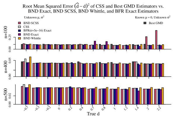
Figure 13: For CSS, BND, and BFR$\left(\epsilon=5\times 10^{-16}\right)$, root mean squared error (RMSE) of estimates of the memory parameter $\hat{d}$ is approximated from $10,000$ simulated ARFIMA$\left(0,d,0\right)$ time series with mean $\mu=0$ and variance $\sigma^{2}=1$ for each sample size $n$ and true value of the differencing parameter $d$. Root mean squared error (RMSE) for the best GMD estimator is reprinted from Mayoral (2007) by choosing the smallest average RMSE across GMD estimators that use a different number of autocorrelations at each value of the true memory parameter $d$ and sample size $n$.

Figure 13 shows that the variability of our adaptive estimators is comparable to the variability of the CSS estimator and the “Best GMD” estimator for most sample sizes and true values of $d$. Again, this is especially noteworthy given that the adaptive BND SCSS, BND exact, and BFR$\left(\epsilon\right)$ exact estimators summarized in Figure 13 treat the overall mean $\mu$ and variance $\sigma^{2}$ as unknown, whereas the version of Mayoral’s estimator summarized in Figure 13 treats the overall mean $\mu$ as constant and known to be equal to $0$ and the variance $\sigma^{2}$ as unknown. There are some exceptions when the sample size is smaller; the adaptive BND SCSS estimator is especially variable when $d\geq 2$ and the adaptive BND exact estimator is especially variable when $0.5<d<1$.

Appendix D Estimation of $\sigma^{2}$ Comparison with Alternatives

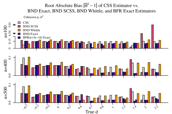
Figure 14: Average absolute bias of estimates of the noise variance $\sigma^{2}$ across $10,000$ simulated ARFIMA$\left(0,d,0\right)$ time series with mean $\mu=0$ and variance $\sigma^{2}=1$ for each sample size $n$ and true value of the differencing parameter $d$.

Appendix E Estimation of $d$ Comparison with Alternatives When Estimating a Polynomial Mean

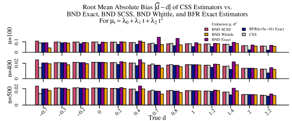
Figure 15: Root average absolute bias of CSS, BND, and BFR$\left(5\times 10^{-16}\right)$ estimators of $d$ across 100 simulated mean-zero ARFIMA$\left(0,d,0\right)$ time series with variance $\sigma^{2}=1$. Estimates are obtained assuming $\mu_{t}=\sum_{j=0}^{2}t^{j}\lambda_{j}$, where $\lambda_{0}$, $\lambda_{1}$, $\lambda_{2}$ and $\sigma^{2}$ are treated as unknown.

Appendix F Estimation of $d$ Comparison with Alternatives for Heavy Tailed Observations

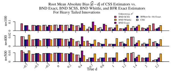
Figure 16: Root average absolute bias of CSS, BND, and BFR$\left(5\times 10^{-16}\right)$ estimators of $d$ across 100 simulated mean-zero time series simulated according to $\left(1-B\right)^{d}y_{t}=z_{t}$, where $z_{t}$ are independent, identically distributed mean zero and unit variance Laplace random variables, which have heavier-than-normal tails. Estimates are obtained assuming $\mu_{t}=\mu$ where $\mu$ and $\sigma^{2}$ are treated as unknown.

Appendix G Estimation of $d$ Comparison with Alternatives for Light Tailed Observations

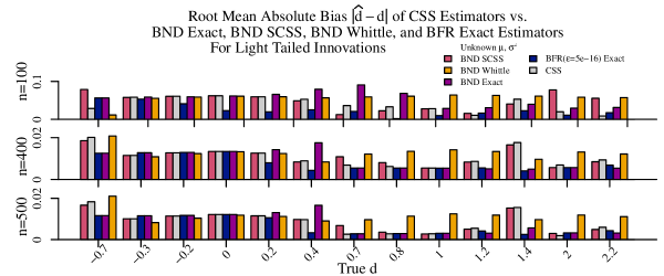
Figure 17: Root average absolute bias of CSS, BND, and BFR$\left(5\times 10^{-16}\right)$ estimators of $d$ across 100 simulated mean-zero time series simulated according to $\left(1-B\right)^{d}y_{t}=z_{t}$, where $z_{t}$ are independent, identically distributed mean zero and unit variance generalized normal random variables with shape parameter 6, which have lighter-than-normal tails. Estimates are obtained assuming $\mu_{t}=\mu$ where $\mu$ and $\sigma^{2}$ are treated as unknown.

Appendix H Estimation of Confidence Intervals

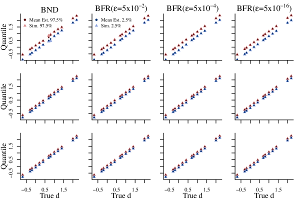
Figure 18: Comparison of lower 2.5% and upper 97.5% quantiles of BND and BFR$\left(\epsilon\right)$ exact likelihood estimators obtained by simulating $10,000$ simulated ARFIMA$\left(0,d,0\right)$ time series with mean $\mu=0$ and variance $\sigma^{2}=1$ versus average lower 2.5% and average upper 97.5% quantiles corresponding to BND and BFR$\left(\epsilon\right)$ exact likelihood estimators obtained using numerical differentiation across $10,000$ simulated ARFIMA$\left(0,d,0\right)$ time series with mean $\mu=0$ and variance $\sigma^{2}=1$ for each sample size $n$ and true value of the differencing parameter $d$.

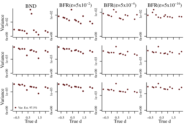
Figure 19: Variance of upper 97.5% quantiles corresponding to BND and BFR$\left(\epsilon\right)$ exact likelihood estimators obtained using numerical differentiation across $10,000$ simulated ARFIMA$\left(0,d,0\right)$ time series with mean $\mu=0$ and variance $\sigma^{2}=1$ for each sample size $n$ and true value of the differencing parameter $d$.

Appendix I Likelihood Instability

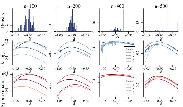
Figure 20: The first row shows histograms of exact maximum likelihood estimates $\hat{d}$ of the differencing parameter $d$ obtained by setting $\bar{d}=3.5$ across a subset of $100$ simulated ARFIMA$\left(0,-0.7,0\right)$ time series with mean $\mu=0$ and variance $\sigma^{2}=1$ for each sample size $n$. The second row shows selected profile log-likelihood curves obtained by setting $\bar{d}=3.5$ for four of the time series depicted in the previous row for each value of $n$. The third row shows approximate profile log-likelihood curves corresponding to the profile log-likelihood curves shown in the previous row obtained by treating values of the time series as conditionally independent after conditioning on the previous 100 values.

Appendix J Chemical Process Concentration and Temperature

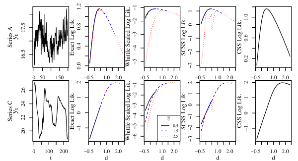
Figure 21: Observed Series A and Series C time series and corresponding exact and Whittle profile log-likelihood curves for $\bar{d}\in\left\{0.5,1.5,2.5\right\}$, with the mean $\mu$ and variance $\sigma^{2}$ profiled out.

			Exact		Whittle	SCSS	CSS
Data	$n$	$\bar{d}$	$\hat{d}_{\bar{d}}$	95% Interval for $d$	$\hat{d}_{\bar{d}}$	$\hat{d}_{\bar{d}}$	$\hat{d}_{\bar{d}}$
Series A	$197$	$0.5$	$0.400$	$\left(0.304,0.496\right)$	$0.420$	$0.418$	$0.418$
		$1.5$	$0.427$	$\left(0.319,0.534\right)$	$0.422$	$0.500$
		$2.5$	$0.436$	$\left(0.326,0.545\right)$	$1.047$	$0.901$
Series C	$226$	$0.5$	$0.500$	$-$	$0.500$	$0.500$	$1.766$
		$1.5$	$1.500$	$-$	$1.500$	$1.500$
		$2.5$	$1.788$	$\left(1.659,1.918\right)$	$1.799$	$1.810$

Table 4: Estimates and corresponding 95% confidence intervals for $d$ for the chemical process concentration readings (Series A) and chemical process temperature readings (Series C) for different values of $\bar{d}$. The BFR$\left(\epsilon=5\times 10^{-16}\right)$ exact likelihood, BND Whittle, and BND SCSS estimates are highlighted in gray. 95% intervals for exact likelihood estimates $\hat{d}_{\bar{d}}$ are provided for values of $\bar{d}$ that correspond to log-likelihoods that are decreasing at $\bar{d}$. The mean $\mu$ and variance $\sigma^{2}$ are treated as unknown when estimating the differencing parameter $d$.

			Exact			Whittle			SCSS			CSS
Data	$n$	$\bar{d}$	$d$	$\theta_{1}$	$\phi_{1}$	$d$	$\theta_{1}$	$\phi_{1}$	$d$	$\theta_{1}$	$\phi_{1}$	$d$	$\theta_{1}$	$\phi_{1}$
Series A	$197$	$0.5$	$0.419$	$-0.037$	$-$	$0.449$	$-0.043$	$-$	0.480	$-0.093$	$-$	$0.479$	$-0.092$	$-$
		$1.5$	$0.502$	$-0.117$	$-$	$0.470$	$-0.077$	$-$	$0.500$	$-0.115$	$-$
		$2.5$	$1.314$	$-0.923$	$-$	$2.047$	$-1.000$	$-$	$0.990$	$-0.685$	$-$
		$3.5$	$1.310$	$-0.911$	$-$	$2.292$	$-0.665$	$-$	$0.994$	$-0.721$	$-$
Series C	$226$	$0.5$	$0.500$	$-$	$1.000$	$0.215$	$-$	$0.907$	$0.500$	$-$	$0.982$	$0.939$	$-$	$0.857$
		$1.5$	$0.950$	$-$	$0.850$	$0.908$	$-$	$0.858$	$0.894$	$-$	$\pagecolor{lightgray}0.881$
		$2.5$	$0.972$	$-$	$0.842$	$0.892$	$-$	$0.930$	$1.014$	$-$	$0.815$
		$3.5$	$0.971$	$-$	$0.852$	$1.109$	$-$	$1.000$	$0.996$	$-$	$0.828$

Table 5: Estimates of the parameters of ARFIMA$\left(0,d,1\right)$ and ARFIMA$\left(1,d,0\right)$ models both with $\mu_{t}=\mu$ for the chemical process concentration readings (Series A) and chemical process temperature readings (Series C) for different values of $\bar{d}$. The BFR$\left(\epsilon=5\times 10^{-16}\right)$ exact likelihood estimates, BND Whittle estimates, and BND SCSS estimates are highlighted in gray. The mean $\mu$ and variance $\sigma^{2}$ are treated as unknown when estimating the differencing parameter $d$.

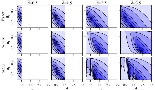
Figure 22: Exact, Whittle, and SCSS joint profile log-likelihoods for Series A as a function of the moving average parameter $\theta_{1}$ and $d$ for $\bar{d}\in\left\{0.5,1.5,2.5,3.5\right\}$, with the mean $\mu$ and variance $\sigma^{2}$ profiled out.

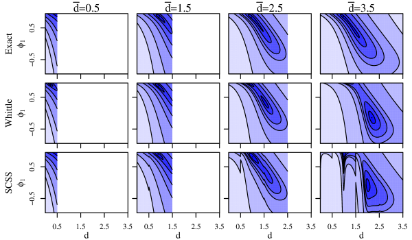
Figure 23: Exact, Whittle, and SCSS joint profile log-likelihoods for Series C as a function of the autoregressive parameter $\phi_{1}$ and $d$ for $\bar{d}\in\left\{0.5,1.5,2.5,3.5\right\}$, with the mean $\mu$ and variance $\sigma^{2}$ profiled out.

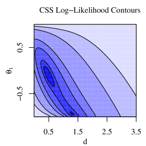
Figure 24: CSS joint profile log-likelihood for Series A as a function of the moving average parameter $\theta_{1}$ and $d$, with the mean $\mu$ and variance $\sigma^{2}$ profiled out.

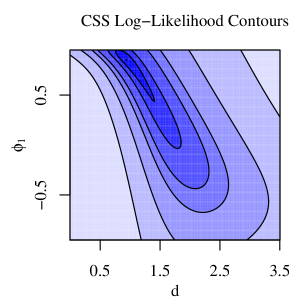
Figure 25: CSS joint profile log-likelihood for Series C as a function of the autoregressive parameter $\phi_{1}$ and $d$, with the mean $\mu$ and variance $\sigma^{2}$ profiled out.

Appendix K Truncated vs. Untruncated Fractional Differences

The model that assumes that truncated fractional differences $\left(1-B\right)^{d}_{+}y_{t}$ are distributed according to a stationary ARMA$\left(p,q\right)$ model and the model that assumes that untruncated fractional differences $\left(1-B\right)^{d}y_{t}$ are distributed according to a stationary ARMA$\left(p,q\right)$ model can both be represented as $y_{t+1}=\sum_{j=1}^{t}c_{tj}y_{t+1-j}+z_{t+1}$, where $z_{t}$ are independent, mean zero random variables with variance $v_{t}$ and the values of $c_{tj}$ and $v_{t}$ are one-step-ahead forecast coefficients and variances determined by which model is being used and its parameters. Comparing the one-step-ahead forecast coefficients and variances across the two models allows us to compare the dependence structure of data generated under the two models. We consider the simpler case where $p=q=0$ and compute the ratios $c_{tj}/\sqrt{v_{t}}$ for $d\in\{-0.5,-0.75,-1,-1.25,-1.5,-1.75\}$ and $t\in\{0,1,2,3\}$. The ratios $c_{tj}/\sqrt{v_{t}}$ are shown in Figure 26. They are similar when $d=-0.5$ but diverge substantially as $d$ decreases. This suggests that when $d\leq-1$, the two models are very different.

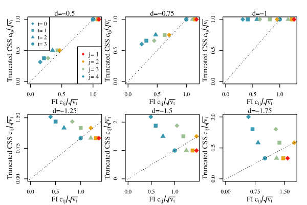
Figure 26: Each panel compares the scaled one-step-ahead forecast coefficients $c_{tj}/\sqrt{v_{t}}$ for the truncated and untruncated fractional difference models for values of $d$ between $-0.5$ and $-1.75$.

References

- Barassi et al. (2018) Barassi, M. R., N. Spagnolo, and Y. Zhao (2018). Fractional Integration Versus Structural Change: Testing the Convergence of CO2 Emissions. Environmental and Resource Economics 71(4), 923–968.
- Beran (1995) Beran, J. (1995). Maximum Likelihood Estimation of the Differencing Parameter for Invertible Short and Long Memory Autoregressive Integrated Moving Average Models. Journal of the Royal Statistical Society. Series B (Methodological) 57(4), 659–672.
- Box and Jenkins (1970) Box, G. E. P. and G. M. Jenkins (1970). Time Series Analysis: Forecasting and Control. San Francisco: Holden Day.
- Box-Steffensmeier and Smith (1998) Box-Steffensmeier, J. M. and R. M. Smith (1998). Investigating Political Dynamics Using Fractional Integration Methods. American Journal of Political Science 42(2), 661–689.
- Byers et al. (1997) Byers, D., J. Davidson, and D. Peel (1997). Modelling political popularity: An analysis of long-range dependence in opinion poll series. Journal of the Royal Statistical Society. Series A: Statistics in Society 160(3), 471–490.
- Byers et al. (2000) Byers, D., J. Davidson, and D. Peel (2000). The dynamics of aggregate political popularity: Evidence from eight countries. Electoral Studies 19(1), 49–62.
- Contreras-Cristán et al. (2006) Contreras-Cristán, A., E. Gutiérrez-Peña, and S. G. Walker (2006). A note on Whittle’s likelihood. Communications in Statistics: Simulation and Computation 35(4), 857–875.
- Dahlhaus (1989) Dahlhaus, R. (1989). Efficient Parameter Estimation for Self-Similar Processes. The Annals of Statistics 17(4), 1749–1766.
- Das and Yang (2020) Das, S. and J. Yang (2020). Spectral methods for small sample time series: A complete periodogram approach. arXiv: 2007.00363.
- Dolado et al. (2003) Dolado, J. J., J. Gonzalo, and L. Mayoral (2003). Long-range dependence in Spanish political opinion poll series. Journal of Applied Econometrics 18(2), 137–155.
- Doornik and Ooms (2003) Doornik, J. A. and M. Ooms (2003). Computational aspects of maximum likelihood estimation of autoregressive fractionally integrated moving average models. Computational Statistics and Data Analysis 42(3), 333–348.
- Durham et al. (2019) Durham, G., J. Geweke, S. Porter-Hudak, and F. Sowell (2019). Bayesian Inference for ARFIMA Models. Journal of Time Series Analysis 40, 388–410.
- Gelsinger et al. (2020) Gelsinger, M. L., L. L. Tupper, and D. S. Matteson (2020). Cell Line Classification Using Electric Cell-Substrate Impedance Sensing (ECIS). International Journal of Biostatistics 16(1), 1–12.
- Giaever and Keese (1991) Giaever, I. and C. R. Keese (1991). Micromotion of mammalian cells measured electrically. Proceedings of the National Academy of Sciences of the United States of America 88(17), 7896–7900.
- Gohbert et al. (1995) Gohbert, I., T. Kailath, and V. Olshevsky (1995). Fast Gaussian Elimination with Partial Pivoting for Matrices with Displacement Structure. Mathematics of Computation 64(212), 1557–1576.
- Granger (1980) Granger, C. W. (1980). Long memory relationships and the aggregation of dynamic models. Journal of Econometrics 14(2), 227–238.
- Hosking (1981) Hosking, J. R. M. (1981). Fractional Differencing. Biometrika 68(1), 165–176.
- Hualde and Nielsen (2020) Hualde, J. and M. Ø. Nielsen (2020). Truncated Sum of Squares Estimation of Fractional Time series Models with Deterministic Trends. Econometric Theory 36(4), 751–772.
- Hualde and Robinson (2011) Hualde, J. and P. M. Robinson (2011). Gaussian pseudo-maximum likelihood estimation of fractional time series models. Annals of Statistics 39(6), 3152–3181.
- Hurvich and Chen (2000) Hurvich, C. M. and W. W. Chen (2000). An Efficient Taper for Potentially Overdifferenced Long-Memory Time Series. Journal of Time Series Analysis 21(2), 155–180.
- Hurvich and Ray (1995) Hurvich, C. M. and B. K. Ray (1995). Estimation of the Memory Parameter For Nonstationary or Noninvertible Fractionally Integrated Processes. Journal of Time Series Analysis 16(1), 17–41.
- Jesus and Chandler (2017) Jesus, J. and R. E. Chandler (2017). Inference with the Whittle Likelihood: A Tractable Approach Using Estimating Functions. Journal of Time Series Analysis 38(2), 204–224.
- Johansen and Nielsen (2016) Johansen, S. and M. Ø. Nielsen (2016). The Role of Initial Values in Conditional Sum-of-Squares Estimation of Nonstationary Fractional Time Series Models. Econometric Theory 32(5), 1095–1139.
- Lieberman et al. (2012) Lieberman, O., R. Rosemarin, and J. Rousseau (2012). Asymptotic Theory for Maximum Likelihood Estimation of the Memory Parameter in Stationary Gaussian Processes. Econometric Theory 28(2), 457–470.
- Mayoral (2007) Mayoral, L. (2007). Minimum distance estimation of stationary and non-stationary ARFIMA processes. Econometrics Journal 10(1), 124–148.
- Nielsen (2015) Nielsen, M. Ø. (2015). Asymptotics for the conditional-sum-of-squares estimator in multivariate fractional time-series models. Journal of Time Series Analysis 36(2), 154–188.
- Odaki (1993) Odaki, M. (1993). On the Invertibility of Fractionally Differenced ARIMA Processes. Biometrika 80(3), 703–709.
- Pipiras and Taqqu (2017) Pipiras, V. and M. S. Taqqu (2017). Long-Range Dependence and Self-Similarity. Cambridge: Cambridge University Press.
- Sowell (1992) Sowell, F. (1992). Maximum likelihood estimation of stationary univariate fractionally integrated time series models. Journal of Econometrics 53, 165–188.
- Sykulski et al. (2019) Sykulski, A. M., S. C. Olhede, A. P. Guillaumin, J. M. Lilly, and J. J. Early (2019). The debiased Whittle likelihood. Biometrika 106(2), 251–266.
- Tarantola et al. (2010) Tarantola, M., A. K. Marel, E. Sunnick, H. Adam, J. Wegener, and A. Janshoff (2010). Dynamics of human cancer cell lines monitored by electrical and acoustic fluctuation analysis. Integrative Biology 2(2-3), 139–150.
- Velasco and Robinson (2000) Velasco, C. and P. M. Robinson (2000). Whittle Pseudo-Maximum Likelihood Estimation for Nonstationary Time Series. Journal of the American Statistical Association 95(452), 1229–1243.
- Zhang et al. (2020) Zhang, W., M. Griffin, and D. Matteson (2020). Modeling Nonlinear Growth Followed by Long-Memory Equilibrium with Unknown Change Point. arXiv: 2007.09417v2.