A Computationally Efficient Classification Algorithm in Posterior Drift Model: Phase Transition and Minimax Adaptivity

Abstract

In massive data analysis, training and testing data often come from very different sources, and their probability distributions are not necessarily identical. A feature example is nonparametric classification in posterior drift model where the conditional distributions of the label given the covariates are possibly different. In this paper, we derive minimax rate of the excess risk for nonparametric classification in posterior drift model in the setting that both training and testing data have smooth distributions, extending a recent work by Cai and Wei, (2019) who only impose smoothness condition on the distribution of testing data. The minimax rate demonstrates a phase transition characterized by the mutual relationship between the smoothness orders of the training and testing data distributions. We also propose a computationally efficient and data-driven nearest neighbor classifier which achieves the minimax excess risk (up to a logarithm factor). Simulation studies and a real-world application are conducted to demonstrate our approach.

Keywords: Transfer Learning, Domain Adaptation, Computational advantage, Adaptive Rate-Optimal

1 Introduction

Despite the significant successes of conventional classification algorithms, one of their unavoidable limitations is to assume that the source (training) data and target (testing) data are identically distributed. In real-world scenarios, it could be difficult and expensive to obtain source data that has the same distribution as the target data (Weiss et al.,, 2016). Thus, an algorithm which can overcome such discrepancy would be highly valuable. Transfer learning is a promising tool to build models for the target domain by transferring data information from the related source domain. In comparison with traditional machine learning algorithms, transfer learning has demonstrated advantages in many aspects such as image classification (Zhu et al.,, 2011; Han et al.,, 2018; Hussain et al.,, 2018), autonomous driving (Kim and Park,, 2017), recommendation system (Zhao et al.,, 2013; Zhang et al.,, 2017), etc. An important transfer learning technique is the so-called domain adaptation (Weiss et al.,, 2016), in which the information or knowledge is adapted from one or more source domains to the target domain. Empirical successes of domain adaptation have attracted increasing attention to the study of its theoretical properties. For example, Ben-David et al., (2007) derive a bound on the generalization error of the classifiers trained from data in the source domain, later extended by Blitzer et al., (2008), Zhang et al., (2012) and Zhao et al., (2018) to the case where the classifiers are trained from both source and target domains. Researchers have also proposed additional structural relationships between the source and target domains, e.g., the covariate shift model with different marginal distributions and the posterior drift model with different conditional distributions, under which the generalization error bounds are successfully established. To name a few, see Shimodaira, (2000); Huang et al., (2007); Sugiyama et al., (2008); Mansour et al., (2012); Hoffman et al., (2018); Kpotufe and Martinet, (2018); Scott et al., (2013); Natarajan et al., (2013); Manwani and Sastry, (2013); Gao et al., (2016); Natarajan et al., (2017); Cannings et al., (2020); Cai and Wei, (2019).

A notable work is Cai and Wei, (2019) who propose a $k$-nearest neighbor ($k$NN) classifier based on the posterior drift model and derive minimax optimality. The $k$-nearest neighbors are detected over the entire source and target data which could be computationally expensive when data size is large. Meanwhile, the theoretical results only involve the smoothness of the target distribution but the impact of the smoothness of the source distributions remains unknown. The aim of this work is to further strengthen the two aspects. Specifically, we propose a more computationally efficient $k$NN classifier that requires detecting the nearest neighbors for local data only. We discover a phase transition phenomenon for the minimax excess risk characterized by the mutual relationship between the smoothness orders of the source and target distributions, which degenerate to Cai and Wei, (2019) in the special case when the smoothness order of the source distributions vanishes. Such a phenomenon provides a more complete understanding on the impact of smooth data distributions in transfer learning. In the following subsection, we describe our contributions in more details. Before that, let us introduce some terminologies and notation.

Terminologies and Notation: Let $\|\mathbf{v}\|^{2}=\mathbf{v}^{\top}\mathbf{v}$ denote the Euclidean norm of the vector $\mathbf{v}$. For two sequences $a_{n}$ and $b_{n}$, we say $a_{n}\lesssim b_{n}$ if $a_{n}\leq cb_{n}$ for some constant $c>0$ and all sufficiently large $n$. For $a>0$, let $\left\lfloor a\right\rfloor$ be the largest integer that less than or equal to $a$. Let $\mathcal{D}=[0,1]^{d}\times\{0,1\}$ and $P,Q$ be probability distributions over $\mathcal{D}$. For $(\mathbf{X},Y)\in\mathcal{D}$, the $d$-dimensional $\mathbf{X}$ is regarded as covariates or features, and $Y$ is the binary label of $\mathbf{X}$. For $(\mathbf{X},Y)$ drawn from $P$ (or $Q$), let $P_{\mathbf{X}}$ (or $Q_{\mathbf{X}}$) denote the marginal probability distribution of $\mathbf{X}$. Define $\eta_{P}(\mathbf{x})=P(Y=1|\mathbf{X}=\mathbf{x})$ and $\eta_{Q}(\mathbf{x})=Q(Y=1|\mathbf{X}=\mathbf{x})$ as the conditional distributions of $Y$ given $\mathbf{X}=\mathbf{x}$ for any $\mathbf{x}\in[0,1]^{d}$. For positive sequences $a_{n}$ and $b_{n}$, we say $a_{n}\lesssim b_{n}$ ($a_{n}\gtrsim b_{n}$) if $a_{n}\leq cb_{n}$ ($a_{n}\geq cb_{n}$) for some $c>0$ and all large enough $n$. We say $a_{n}\asymp b_{n}$ if $a_{n}\lesssim b_{n}$ and $a_{n}\gtrsim b_{n}$. We use $\textrm{supp}(\mu)$ to denote the support of the a probability measure $\mu$.

1.1 Nonparametric classification in posterior drift model

Suppose that $(\mathbf{X}_{1}^{P},Y_{1}^{P}),\ldots,(\mathbf{X}_{n_{P}}^{P},Y_{n_{P}}^{P})$ are $n_{P}$ i.i.d. observations from $P$, and $(\mathbf{X}_{1}^{Q},Y_{1}^{Q}),\ldots,$ $(\mathbf{X}_{n_{Q}}^{Q},Y_{n_{Q}}^{Q})$ are $n_{Q}$ i.i.d. observations from $Q$. Moreover, we assume these observations from $P$ and $Q$ are mutually independent. For simplicity, we call $\{(\mathbf{X}_{i}^{P},Y_{i}^{P})\}_{i=1}^{n_{P}}$ the $P$-data and $\{(\mathbf{X}_{i}^{Q},Y_{i}^{Q})\}_{i=1}^{n_{Q}}$ the $Q$-data. Given future covariates $\mathbf{X}$ from $Q_{\mathbf{X}}$, we are interested in predicting its unknown binary label $Y$ based on the full training data $\mathcal{Z}$, where

$$\mathcal{Z}=\{(\mathbf{X}_{1}^{P},Y_{1}^{P}),\ldots,(\mathbf{X}_{n_{P}}^{P},Y_{n_{P}}^{P}),(\mathbf{X}_{1}^{Q},Y_{1}^{Q}),\ldots,(\mathbf{X}_{n_{Q}}^{Q},Y_{n_{Q}}^{Q})\}.$$ (1.1)

We adopt the posterior drift model proposed by Scott, (2019), in which $P_{\mathbf{X}}$ and $Q_{\mathbf{X}}$ have common supports, whereas the conditional distributions of $Y$ given $\mathbf{X}$ under $P,Q$, namely $\eta_{P}$ and $\eta_{Q}$, are possibly different. In this model, $P$ is the source distribution and $Q$ is the target distribution. This model has been recently adopted by Cai and Wei, (2019) in nonparametric classification who proposed an optimal adaptive $k$NN classifier. Since their method requires identifying the nearest covariates among all covariates in $\mathcal{Z}$, which requires $n_{P}+n_{Q}$ attempts and might be computationally expensive. The computational cost easily scales up when the training data consists of observations from multiple distributions. Hence, it is interesting to design a more efficient algorithm that can achieve the same optimality.

1.2 Our Contributions

Our first contribution is to propose a more computationally efficient adaptive $k$-NN classifier, i.e., Algorithm 1 in Section 2. Notably, our method requires $\max\{n_{P},n_{Q}\}$ attempts to identify the nearest covariates. Consequently, the ratio of attempts required by Cai and Wei, (2019) and Algorithm 1 is $\frac{n_{P}+n_{Q}}{\max\{n_{P},n_{Q}\}}$, which is nearly 2 if $n_{P}\approx n_{Q}$ (see Figure 1). In other words, when $P$-data and $Q$-data have equal amount of data points, Algorithm 1 only requires nearly half computational cost of Cai and Wei, (2019). The ratio of attempts further increases if more source distributions are involved, hence, the computational cost of our method, compared to Cai and Wei, (2019), will be further reduced. See discussions in Section 3.3.

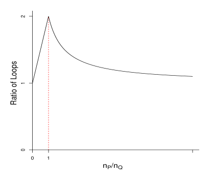
Figure 1: The ratio of attempts required by Cai and Wei, (2019) and Algorithm 1.

Our second contribution is in theoretical aspect. We establish exact orders for the minimax excess risk when $(\eta_{P},\eta_{Q})$ are $(\beta_{P},\beta_{Q})$-Hölder smooth (see Assumption A2). In contrast, Cai and Wei, (2019) established exact orders for the minimax excess risk in the special case $\beta_{P}=0$. It turns out that when $\beta_{P}>0$, the minimax rate has a faster order, demonstrating the advantage of utilizing smooth source distributions. To describe our findings, consider $n_{Q}=0$ for simplicity. Below is a summary of the results in which the orders for the minimax excess risk demonstrate a phase transition characterized by a mutual relationship between $\beta_{P}$ and $\beta_{Q}$:

$$\textrm{the minimax excess risk}\asymp\left\{\begin{array}[]{cc}n_{P}^{-\frac{(1+\alpha)\beta_{Q}}{\gamma(2\beta_{P}+d)}},&\textrm{if $\gamma\beta_{Q}\leq\beta_{P}\leq\gamma d/\alpha$,}\\ n_{P}^{-\frac{(1+\alpha)\beta_{Q}}{2\gamma\beta_{Q}+d}},&\textrm{if $\beta_{P}<\gamma\beta_{Q}\leq\gamma d/\alpha$,}\end{array}\right.$$ (1.2)

where $\alpha>0$ quantifies the Tsybakov noise level (see Assumption A3) and $\gamma>0$ measures the relative signal strength of $P$ and $Q$ (see Assumption A5). See Figure 2(a) for an illustration of (1.2). Note that (1.2) excludes the regions $\beta_{P}>\gamma d/\alpha$ and $\beta_{Q}>d/\alpha$ in which only upper bounds on the minimax excess risk are available. Interestingly, the upper bounds are super fast $(\lesssim n_{P}^{-1})$, see Figure 2(b), which is consistent to the findings of Audibert and Tsybakov, (2007). The orders of the minimax excess risk are fast $(\lesssim n_{P}^{-1/2})$ or in a nonparametric rate ($\gtrsim n_{P}^{-1/2}$) in other domains of $(\beta_{P},\beta_{Q})$. The results are further extended to general $n_{Q}$ in Section 3.2, and to multiple source distributions in Section 3.3.

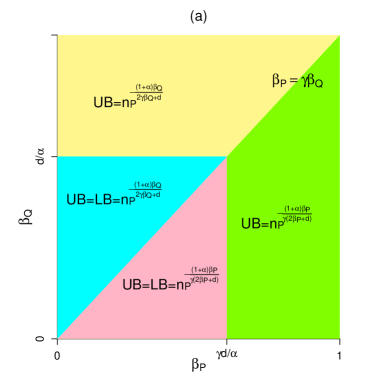
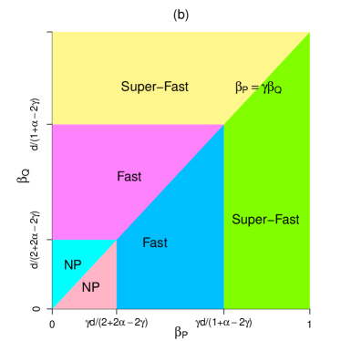
Figure 2: (a). Upper bounds (UB) and lower bounds (LB) of the minimax excess risk in different domains of $(\beta_{P},\beta_{Q})$. (b). Categories of the excess risk bounds characterized by $(\beta_{P},\beta_{Q})$. NP: nonparametric rate $(\gtrsim n_{P}^{-1/2})$; Fast: fast rate $(\lesssim n_{P}^{-1/2})$; Super-Fast: super-fast rate $(\lesssim n_{P}^{-1})$.

2 A Computationally Efficient Adaptive $k$NN Classifier

In this section, we propose a computationally efficient adaptive $k$NN classifier. For any $\mathbf{x}\in[0,1]^{d}$, $1\leq k_{P}\leq n_{P}$ and $1\leq i\leq k_{P}$, let $\mathbf{X}_{(i)}^{P}(\mathbf{x})$ denote the $i$th nearest covariate of $\mathbf{x}$ among $\mathbf{X}_{1}^{P},\mathbf{X}_{2}^{P},\ldots,\mathbf{X}_{n_{P}}^{P}$, and let $Y_{(i)}^{P}(\mathbf{x})$ denote the label of $\mathbf{X}_{(i)}^{P}(\mathbf{x})$. One can similarly define $\mathbf{X}_{(i)}^{Q}(\mathbf{x})$ and $Y_{(i)}^{Q}(\mathbf{x})$. Let

$$\widehat{\eta}_{k_{P}}(\mathbf{x})=\frac{1}{k_{P}}\sum_{i=1}^{k_{P}}Y_{(i)}^{P}(\mathbf{x}),\,\,\,\,\,\,\,\,\widehat{\eta}_{k_{Q}}(\mathbf{x})=\frac{1}{k_{Q}}\sum_{i=1}^{k_{Q}}Y_{(i)}^{Q}(\mathbf{x}).$$ (2.1)

Here $\widehat{\eta}_{k_{P}}(\mathbf{x})$ ($\widehat{\eta}_{k_{Q}}(\mathbf{x})$) is the $k$NN estimator of $\eta_{P}(\mathbf{x})$ ($\eta_{Q}(\mathbf{x})$) based on the $P$-data ($Q$-data). Inspired from Cai and Wei, (2019), we can aggregate $\widehat{\eta}_{k_{P}}$ and $\widehat{\eta}_{k_{Q}}$ into a weighted $k$NN estimator:

$$\widehat{\eta}_{NN}(\mathbf{x})=\frac{w_{P}k_{P}\widehat{\eta}_{k_{P}}(\mathbf{x})+w_{Q}k_{Q}\widehat{\eta}_{k_{Q}}(\mathbf{x})}{w_{P}k_{P}+w_{Q}k_{Q}},$$

where $w_{P},w_{Q}$ are positive weights. The corresponding $k$NN classifier $\widehat{f}_{NN}$ is then defined as

$$\widehat{f}_{NN}(\mathbf{x})\mathrel{\mathop{\mathchar 58\relax}}=\mathbb{I}(\widehat{\eta}_{NN}(\mathbf{x})\geq 1/2)=\begin{cases}1,&\textrm{ if }\widehat{\eta}_{NN}(\mathbf{x})\geq 1/2,\\ 0,&\textrm{ if }\widehat{\eta}_{NN}(\mathbf{x})<1/2,\end{cases}\,\,\,\,\,\,\,\,\textrm{for any $\mathbf{x}\in[0,1]^{d}$.}$$ (2.2)

A limitation of $\widehat{f}_{NN}$ is that it requires predetermined $k_{P},k_{Q},w_{P},w_{Q}$. To address this, we propose Algorithm 1 in which the parameters are data-driven.

Input: $P$-data $(\mathbf{X}_{1}^{P},Y_{1}^{P}),\ldots,(\mathbf{X}_{n_{P}}^{P},Y_{n_{P}}^{P})$, $Q$-data $(\mathbf{X}_{1}^{Q},Y_{1}^{Q}),\ldots,(\mathbf{X}_{n_{Q}}^{Q},Y_{n_{Q}}^{Q})$ with $n_{P}\geq n_{Q}$, and new features $\mathbf{x}$;

Initiation: set $k_{P}=0$;

while $k_{P}<n_{P}$ do

      update $k_{P}\mathrel{\mathop{\mathchar 58\relax}}=k_{P}+1$ and $k_{Q}\mathrel{\mathop{\mathchar 58\relax}}=\left\lfloor k_{P}n_{Q}/n_{P}\right\rfloor$;

      calculate $\widehat{\eta}_{k_{P}}$ and $\widehat{\eta}_{k_{Q}}(\mathbf{x})$ (set $\widehat{\eta}_{k_{Q}}(\mathbf{x})=1/2$ if $k_{Q}=0$);

      calculate

      $r_{k_{P}}=\begin{cases}\sqrt{k_{P}(\widehat{\eta}_{k_{P}}(\mathbf{x})-1/2)^{2}+k_{Q}(\widehat{\eta}_{k_{Q}}(\mathbf{x})-1/2)^{2}}&\textrm{ if }sign(\widehat{\eta}_{k_{P}}(\mathbf{X})-1/2)=sign(\widehat{\eta}_{k_{Q}}(\mathbf{X})-1/2);\\ \max\{\sqrt{k_{P}}|\widehat{\eta}_{k_{P}}(\mathbf{x})-1/2|,\sqrt{k_{Q}}|\widehat{\eta}_{k_{Q}}(\mathbf{x})-1/2|\}&\textrm{ if }sign(\widehat{\eta}_{k_{P}}(\mathbf{x})-1/2)\neq sign(\widehat{\eta}_{k_{Q}}(\mathbf{x})-1/2);\\ \end{cases}$

      if $r_{k_{P}}>\sqrt{[d+\log(n_{P}+n_{q})]\log(n_{P}+n_{q})}$ or $k_{P}=n_{P}$ then

          set $\widehat{k}_{P}=k_{P}$ and $\widehat{k}_{Q}=k_{Q}$;

          exit loop;

      end if

end while

calculate $\widehat{\eta}_{\widehat{k}_{P}}(\mathbf{x})$, $\widehat{\eta}_{\widehat{k}_{Q}}(\mathbf{x})$;

Output: classifier $\widehat{f}_{pa}(\mathbf{x})=\mathbb{I}({k_{P}}(\widehat{\eta}_{\widehat{k}_{P}}(\mathbf{x})-1/2)+{k_{Q}}(\widehat{\eta}_{\widehat{k}_{Q}}(\mathbf{x})-1/2)\geq 0)$.

Algorithm 1 An Adaptive $k$NN Algorithm

To ease presentation, Algorithm 1 has only considered $n_{P}\geq n_{Q}$. When $n_{P}<n_{Q}$, by flipping $n_{P}$ and $n_{Q}$ we can set $k_{P}=\left\lfloor k_{Q}n_{P}/n_{Q}\right\rfloor$ during the loops until the same stopping rule is met. Below we discuss the intuition why Algorithm 1 performs optimal. Let $\rho=\frac{w_{P}k_{P}}{w_{P}k_{P}+w_{Q}k_{Q}}$, so we can rewrite $\widehat{\eta}_{NN}$ as $\widehat{\eta}_{NN}(\mathbf{x})=\rho\widehat{\eta}_{k_{P}}(\mathbf{x})+(1-\rho)\widehat{\eta}_{k_{Q}}(\mathbf{x})$, whose “signal,” defined as the absolute deviation from random guess, and “standard deviation” are given as $|\widehat{\eta}_{NN}(\mathbf{x})-1/2|$ and $\sqrt{\rho^{2}/k_{P}+(1-\rho)^{2}/k_{Q}}$, respectively. During each loop, Algorithm 1 finds the “optimal” $\rho$ that minimizes the “signal-to-noise” ratio:

$$\widehat{\rho}=\mathop{\mathrm{argmin}}_{\rho}\frac{|\widehat{\eta}_{NN}(\mathbf{x})-1/2|}{\sqrt{\rho^{2}/k_{P}+(1-\rho)^{2}/k_{Q}}}.$$ (2.3)

By direct calculations, the minimal value of (2.3) is $r_{k_{P}}$ which is achieved at $\rho=\widehat{\rho}$. Therefore, Algorithm 1 scans the first $k_{P}$ such that the minimal “signal-to-noise” ratio $r_{k_{P}}$ is greater than a threshold $\sqrt{[d+\log(n_{P}+n_{q})]\log(n_{P}+n_{q})}$. The choice of such threshold is inspired from Cai and Wei, (2019), under which it can be shown that, with high probability, $\mathbb{E}(\widehat{\eta}_{NN}(\mathbf{x})|\mathcal{X})$ and $\widehat{\eta}_{NN}(\mathbf{x})$ have the same sign. Here $\mathcal{X}\mathrel{\mathop{\mathchar 58\relax}}=\{\mathbf{X}_{1}^{P},\ldots,\mathbf{X}_{n_{P}}^{P},\mathbf{X}_{1}^{Q},\ldots,\mathbf{X}_{n_{Q}}^{Q}\}$ is the collection of all covariates. Under assumptions in Section 3, is can be shown that $\mathbb{E}(\widehat{\eta}_{NN}(\mathbf{x})|\mathcal{X})$ has the same sign as $\eta_{Q}(\mathbf{x})$, so $\widehat{\eta}_{NN}(\mathbf{x})$ is asymptotically optimal.

To conclude this section, we briefly discuss the computing advantage of our method. In Algorithm 1, $(k_{P},k_{Q})$ is selected over $\{(k_{P},k_{Q})\mathrel{\mathop{\mathchar 58\relax}}k_{Q}=\left\lfloor k_{P}n_{Q}/n_{P}\right\rfloor,1\leq k_{P}\leq\max\{n_{P},n_{Q}\}\}$ which requires $\max\{n_{P},n_{Q}\}$ attempts. In contrast, Cai and Wei, (2019) selects $(k_{P},k_{Q})$ over a set of cardinality $n_{P}+n_{Q}$, hence, requires $n_{P}+n_{Q}$ attempts. Therefore, Algorithm 1 is computationally more feasible than Cai and Wei, (2019).

3 Asymptotic Theory

In this section, we explore the asymptotic properties of $\widehat{f}_{NN}$ in (2.2) and $\widehat{f}_{pa}$ provided in Algorithm 1. We start from the easier case $n_{Q}=0$, and proceed to the general case $n_{Q}\neq 0$.

3.1 Minimax Rate for the Excess Risk when $n_{Q}=0$

When $n_{Q}=0$, we have $\widehat{f}_{NN}(\mathbf{x})=\mathbb{I}(\widehat{\eta}_{k_{P}}(\mathbf{x})\geq 1/2)$, where $\widehat{\eta}_{k_{P}}(\mathbf{x})$ is given in (2.1). Meanwhile, by (2.3) we have $\widehat{\rho}=1$. Thus, Algorithm 1 becomes the following Algorithm 2.

Input: $P$-data $(\mathbf{X}_{1}^{P},Y_{1}^{P}),\ldots,(\mathbf{X}_{n_{P}}^{P},Y_{n_{P}}^{P})$ and new features $\mathbf{x}$;

Initiation: set $k_{P}=0$;

while $k_{P}<n_{P}$ do

      update $k_{P}\mathrel{\mathop{\mathchar 58\relax}}=k_{P}+1$;

      calculate $\widehat{\eta}_{k_{P}}(\mathbf{x})=\frac{1}{k_{P}}\sum_{i=1}^{k_{P}}Y_{(i)}^{P}(\mathbf{x})$;

      calculate $r_{k_{P}}=\sqrt{k_{P}}|\widehat{\eta}_{k_{P}}(\mathbf{x})-1/2|$;

      if $r_{k_{P}}>\sqrt{[d+\log(n_{P})]\log(n_{P})}$ or $k=n_{P}$ then

          set $\widehat{k}_{P}=k_{P}$;

          exit loop;

      end if

end while

calculate $\widehat{\eta}_{\widehat{k}_{P}}(\mathbf{x})$;

Output: classifier $\widehat{f}_{pa}(\mathbf{x})=\mathbb{I}(\widehat{\eta}_{\widehat{k}_{P}}(\mathbf{x})\geq 1/2)$.

Algorithm 2 An Adaptive $k$NN Algorithm under $n_{Q}=0$

Before investigating the asymptotic properties of the above classifiers, we introduce some technical assumptions. Throughout, let $\lambda$ denote the Lebesgue measure on $\mathbb{R}^{d}$.

Assumption A1.

(Common Support and Strong Density) There exist an $\Omega\subset[0,1]^{d}$ and constants $c_{\lambda},r_{\lambda}>0$ such that

1. $\Omega$ is the common support of the marginal distributions $P_{\mathbf{X}}$ and $Q_{\mathbf{X}}$;

2. $\lambda[\Omega\cap B(\mathbf{x},r)]\geq c_{\lambda}\lambda[B(\mathbf{x},r)]$ for all $0<r<r_{\lambda}$ and $\mathbf{x}\in\Omega$;

3. $c_{\lambda}<\frac{dP_{\mathbf{X}}}{d\lambda}(\mathbf{x})<c_{\lambda}^{-1}$ and $c_{\lambda}<\frac{dQ_{\mathbf{X}}}{d\lambda}(\mathbf{x})<c_{\lambda}^{-1}$, for all $\mathbf{x}\in\Omega$.

Assumption A2.

(Hölder Smoothness) There exist constants $C_{\beta}>0$ and $\beta_{P},\beta_{Q}\in[0,1]$ with $\max(\beta_{P},\beta_{Q})>0$ such that $(\eta_{P},\eta_{Q})$ are $(\beta_{P},\beta_{Q})$-Hölder smooth, i.e., $|\eta_{P}(\mathbf{x}_{1})-\eta_{P}(\mathbf{x}_{2})|\leq C_{\beta}\|\mathbf{x}_{1}-\mathbf{x}_{2}\|^{\beta_{P}}$ and $|\eta_{Q}(\mathbf{x}_{1})-\eta_{Q}(\mathbf{x}_{2})|\leq C_{\beta}\|\mathbf{x}_{1}-\mathbf{x}_{2}\|^{\beta_{Q}}$ for all $\mathbf{x}_{1},\mathbf{x}_{2}\in\Omega$.

Assumption A3.

(Tsybakov’s Noise Condition) There exist constants $\alpha\geq 0$ and $C_{\alpha}>0$ such that, for all $t\in(0,1/2]$, $Q_{\mathbf{X}}(|\eta_{Q}(\mathbf{X})-1/2|<t)\leq C_{\alpha}t^{\alpha}$.

Assumption A4.

(Relative Signal Exponent Condition) For all $\mathbf{x}\in\Omega$, it holds that

1. $(\eta_{P}(\mathbf{x})-1/2)(\eta_{Q}(\mathbf{x})-1/2)\geq 0$;

2. $|\eta_{P}(\mathbf{x})-1/2|\geq C_{\gamma}|\eta_{Q}(\mathbf{x})-1/2|^{\gamma}$ for some constants $\gamma,C_{\gamma}>0$.

Assumption A1 consists of three aspects. Assumption A1(a) requires supp($Q_{\mathbf{X}}$)$=$supp($P_{\mathbf{X}}$) which can be relaxed to supp($Q_{\mathbf{X}}$)$\subset$ supp($P_{\mathbf{X}}$) with a slight modification in the proof. The latter is necessary since otherwise there will be a covariate in supp($Q_{\mathbf{X}}$)$\backslash$ supp($P_{\mathbf{X}}$) which is unpredictable by the $P$-data. Assumptions A1(b) and A1(c) are the so-called Strong Density Assumption commonly used in literature (see Audibert and Tsybakov,, 2007). Assumption A1(b) regularizes the feature space $\Omega$. Assumption A1(c) assumes that the densities of $P_{\mathbf{X}}$ and $Q_{\mathbf{X}}$ are bounded away from zero and infinity.

Assumption A2 requires that $\eta_{P}$ and $\eta_{Q}$ are Hölder smooth with orders $\beta_{P}$ and $\beta_{Q}$, which includes the special case $\beta_{P}=0$ in Cai and Wei, (2019). Assumption A3 is the so-called Tsybakov noise condition with a noise exponent $\alpha$ (see Mammen et al.,, 1999; Audibert and Tsybakov,, 2007). Assumption A4, firstly introduced by Cai and Wei, (2019), consists of two parts. Assumption A4(a) requires that the Bayes classifiers $f_{P}^{*}(\cdot)=\mathbb{I}(\eta_{P}(\cdot)\geq 1/2)$ and $f_{Q}^{*}(\cdot)=\mathbb{I}(\eta_{Q}(\cdot)\geq 1/2)$ are essentially the same. Assumption A4(b) measures the relative signal strength of $P$ and $Q$. Similar assumption is also proposed by Hanneke and Kpotufe, (2019).

Recall that the excess risk of $\widehat{f}_{NN}$ under $Q$ is defined as

$$\mathcal{R}_{Q}(\widehat{f}_{NN})=\mathbb{E}(\mathcal{E}_{Q}(\widehat{f}_{NN}))-\mathcal{E}_{Q}(f^{*}_{Q}),$$

where $\mathcal{E}_{Q}(f)=Q(f(\mathbf{X})\neq Y)$ is the classification risk of classifier $f\mathrel{\mathop{\mathchar 58\relax}}\Omega\to\{0,1\}$ under $Q$, and $f_{Q}^{*}$ is the Bayes classifier defined as $f_{Q}^{*}(\cdot)=\mathbb{I}(\eta_{Q}(\cdot)\geq 1/2)$. Let $\Pi(\theta)$ be the collection of $(P,Q)$ satisfying Assumptions A1-A4, where $\theta=\{\alpha,\beta_{P},\beta_{Q},\gamma,c_{\lambda},r_{\lambda},C_{\beta},C_{\alpha},C_{\gamma}\}$ is the collection of constants in the statements of the above assumptions. Based on the above assumptions and notation, the following theorem provides upper bounds for the excess risk of $\widehat{f}_{NN}$ and $\widehat{f}_{pa}$ in the special case $n_{Q}=0$.

Theorem 1.

The following statements hold when $n_{Q}=0$:

1. If $\beta_{P}>\gamma\beta_{Q}$ and $k_{P}\asymp n_{P}^{\frac{2\beta_{P}}{2\beta_{P}+d}}$, then $\sup_{(P,Q)\in\Pi(\theta)}\mathcal{R}_{Q}(\widehat{f}_{NN})\lesssim n_{P}^{-\frac{(1+\alpha)\beta_{P}}{\gamma(2\beta_{P}+d)}}$;

2. If $\beta_{P}\leq\gamma\beta_{Q}$ and $k_{P}\asymp n_{P}^{\frac{2\gamma\beta_{Q}}{2\gamma\beta_{Q}+d}}$, then $\sup_{(P,Q)\in\Pi(\theta)}\mathcal{R}_{Q}(\widehat{f}_{NN})\lesssim n_{P}^{-\frac{(1+\alpha)\beta_{Q}}{2\gamma\beta_{Q}+d}}$.

Moreover, the following holds for the classifier proposed in Algorithm 2:

1. If $\beta_{P}>\gamma\beta_{Q}$, then $\sup_{(P,Q)\in\Pi(\theta)}\mathcal{R}_{Q}(\widehat{f}_{\textrm{pa}})\lesssim\left(\frac{n_{P}}{\log^{2}(n_{P})}\right)^{-\frac{(1+\alpha)\beta_{P}}{\gamma(2\beta_{P}+d)}}$;

2. If $\beta_{P}\leq\gamma\beta_{Q}$, then $\sup_{(P,Q)\in\Pi(\theta)}\mathcal{R}_{Q}(\widehat{f}_{\textrm{pa}})\lesssim\left(\frac{n_{P}}{\log^{2}(n_{P})}\right)^{-\frac{(1+\alpha)\beta_{Q}}{2\gamma\beta_{Q}+d}}$.

Theorem 1 provides upper bounds for the excess risk of $\widehat{f}_{NN}$ and $\widehat{f}_{pa}$ over $(P,Q)\in\Pi(\theta)$ in two smoothness scenarios: $\beta_{P}>\gamma\beta_{Q}$ and $\beta_{P}\leq\gamma\beta_{Q}$. Up to logarithmic sacrifice, $\widehat{f}_{pa}$ performs equally well as $\widehat{f}_{NN}$. When $\gamma$ is small, all upper bounds become smaller, indicating that more information has been transferred from $P$ to $Q$ to boost the classification performance.

Under certain circumstances, the excess risk has a very fast convergence rate. For instance, the excess risk is faster than $n_{P}^{-1/2}$ if $\beta_{P}>\gamma\beta_{Q}$ and $2(1+\alpha-\gamma)\beta_{P}\geq\gamma d$, or $\beta_{P}\leq\gamma\beta_{Q}$ and $2(1+\alpha-\gamma)\beta_{Q}\geq d$; it is faster than $n_{P}^{-1}$ if $\beta_{P}>\gamma\beta_{Q}$ and $(1+\alpha-2\gamma)\beta_{P}\geq\gamma d$, or $\beta_{P}\leq\gamma\beta_{Q}$ and $2(1+\alpha-\gamma)\beta_{Q}\geq d$. It is easy to see that these results degenerate to Audibert and Tsybakov, (2007) in the conventional setting $P=Q$ and $\gamma=1$. Our findings are summarized in Figure 2(b).

The following theorem provides the minimax lower bounds for the excess risk.

Theorem 2.

If $n_{Q}=0$, then the following statements hold:

1. If $\beta_{P}>\gamma\beta_{Q}$ and $\alpha\beta_{P}\leq\gamma d$, then $\inf_{\widehat{f}}\sup_{(P,Q)\in\Pi(\theta)}\mathcal{R}_{Q}(\widehat{f})\geq cn_{P}^{-\frac{(1+\alpha)\beta_{P}}{\gamma(2\beta_{P}+d)}}$;

2. If $\beta_{P}\leq\gamma\beta_{Q}$ and $\alpha\beta_{Q}\leq d$, then $\inf_{\widehat{f}}\sup_{(P,Q)\in\Pi(\theta)}\mathcal{R}_{Q}(\widehat{f})\geq cn_{P}^{-\frac{(1+\alpha)\beta_{Q}}{2\gamma\beta_{Q}+d}}$,

where $c$ is a positive constant relying on $\theta$, and the infimum is taken over classifiers constructed on the $P$-data.

We emphasize that the conditions $\alpha\beta_{P}\leq\gamma d$ and $\alpha\beta_{Q}\leq d$ are necessary to obtain minimax lower bounds. In fact, in the special case $P=Q$, we have $\beta_{P}=\beta_{Q}$ and $\gamma=1$, so both conditions reduce to $\alpha\beta_{Q}\leq d$, which was used by Audibert and Tsybakov, (2007) to establish the minimax lower bounds for the excess risk. Without assuming $\alpha\beta_{Q}\leq d$, the minimax lower bound remains unknown (see Andrea and Samory,, 2017).

Combining Theorem 1 and Theorem 2, we immediately have the following conclusion:

1. If $\beta_{P}>\gamma\beta_{Q}$ and $\alpha\beta_{P}\leq\gamma d$, then $\inf_{\widehat{f}}\sup_{(P,Q)\in\Pi(\theta)}\mathcal{R}_{Q}(\widehat{f})\asymp n_{P}^{-\frac{(1+\alpha)\beta_{P}}{\gamma(2\beta_{P}+d)}}$;

2. If $\beta_{P}\leq\gamma\beta_{Q}$ and $\alpha\beta_{Q}\leq d$, then $\inf_{\widehat{f}}\sup_{(P,Q)\in\Pi(\theta)}\mathcal{R}_{Q}(\widehat{f})\asymp n_{P}^{-\frac{(1+\alpha)\beta_{Q}}{2\gamma\beta_{Q}+d}}$.

Consequently, $\widehat{f}_{NN}$ and $\widehat{f}_{pa}$ both achieve the minimax optimal convergence rate. The optimal rate does not change when $\beta_{P}\in[0,\gamma\beta_{Q}]$, while it tends to zero faster when $\beta_{Q}\in(\gamma\beta_{Q},1]$. The above conclusions are summarized in Figure 2(a) in which a phase transition phenomenon is observed.

3.2 Extensions to General $n_{Q}$

We extend the results in Section 3.1 to general $n_{Q}$. We need the following assumption, a stronger version of Assumption A4.

Assumption A5.

(Mutual Relative Signal Exponent Condition) For all $\mathbf{x}\in\Omega$, it holds that

1. $(\eta_{P}(\mathbf{x})-1/2)(\eta_{Q}(\mathbf{x})-1/2)\geq 0$;

2. $C_{\gamma}|\eta_{Q}(\mathbf{x})-1/2|^{\gamma}\leq|\eta_{P}(\mathbf{x})-1/2|\leq C_{\gamma}^{-1}|\eta_{Q}(\mathbf{x})-1/2|^{\gamma}$ for some constants $\gamma,0<C_{\gamma}<1$.

Assumption A5 requires an additional upper bound $|\eta_{P}(\mathbf{x})-1/2|\leq C_{\gamma}^{-1}|\eta_{Q}(\mathbf{x})-1/2|^{\gamma}$ in comparison with Assumption A4. After rewriting this bound as $|\eta_{Q}(\mathbf{x})-1/2|\geq C_{\gamma}^{1/\gamma}|\eta_{P}(\mathbf{x})-1/2|^{1/\gamma}$, we can see the additional condition essentially requires $1/\gamma$ being the relative signal exponent of $Q$ with respective to $P$, which assesses the information that can be transferred from $Q$ to $P$ (see the discussion right after Theorem 1). Therefore, it is reasonable to view $\gamma$ as the mutual relative signal exponent.

Let $\Pi^{\prime}(\theta)$ be the collection of $(P,Q)$ satisfying Assumptions A1, A2, A3 and A5, where $\theta=\{\alpha,\beta_{P},\beta_{Q},\gamma,c_{\lambda},r_{\lambda},C_{\beta},C_{\alpha},C_{\gamma}\}$ is the collection of constants involved in the corresponding assumptions. Clearly, $\Pi^{\prime}(\theta)$ is a subset of $\Pi(\theta)$. The following theorem extends the results in Theorem 1 to general $n_{Q}$.

Theorem 3.

Suppose that either $n_{Q}\to\infty$ or $n_{P}\to\infty$. Then the following statements hold:

1. If $\beta_{P}>\gamma\beta_{Q}$, $w_{Q}\asymp\delta$, $w_{P}\asymp\delta^{\gamma},k_{Q}\asymp n_{Q}\delta^{\frac{\gamma d}{\beta_{P}}}$, and $k_{P}\asymp n_{P}\delta^{\frac{\gamma d}{\beta_{P}}}$, where $\delta=(n_{P}^{\frac{2\beta_{P}+\gamma d}{\gamma(2\beta_{P}+d)}}+n_{Q})^{-\frac{\beta_{P}}{2\beta_{P}+\gamma d}}$, then

   $$\sup_{(P,Q)\in\Pi^{\prime}(\theta)}\mathcal{R}_{Q}(\widehat{f}_{NN})\lesssim(n_{P}^{\frac{2\beta_{P}+\gamma d}{\gamma(2\beta_{P}+d)}}+n_{Q})^{-\frac{\beta_{P}(1+\alpha)}{2\beta_{P}+\gamma d}};$$ (3.1)

2. If $\beta_{P}\leq\gamma\beta_{Q}$, $w_{Q}\asymp\delta,w_{P}\asymp\delta^{\gamma},k_{Q}\asymp n_{Q}\delta^{\frac{d}{\beta_{Q}}}$, and $k_{P}\asymp n_{P}\delta^{\frac{d}{\beta_{Q}}}$, where $\delta=(n_{P}^{\frac{2\beta_{Q}+d}{2\gamma\beta_{Q}+d}}+n_{Q})^{-\frac{\beta_{Q}}{2\beta_{Q}+d}}$, then

   $$\sup_{(P,Q)\in\Pi(\theta)}\mathcal{R}_{Q}(\widehat{f}_{NN})\lesssim(n_{P}^{\frac{2\beta_{Q}+d}{2\gamma\beta_{Q}+d}}+n_{Q})^{-\frac{\beta_{Q}(1+\alpha)}{2\beta_{Q}+d}}.$$ (3.2)

Moreover, the adaptive classifier proposed in Algorithm 1 has the following properties:

1. If $\beta_{P}>\gamma\beta_{Q}$, then

   $$\sup_{(P,Q)\in\Pi^{\prime}(\theta)}\mathcal{R}_{Q}(\widehat{f}_{pa})\lesssim\bigg{[}\bigg{(}\frac{n_{P}}{\log^{2}(n_{P}+n_{Q})}\bigg{)}^{\frac{2\beta_{P}+\gamma d}{\gamma(2\beta_{P}+d)}}+\frac{n_{P}}{\log^{2}(n_{P}+n_{Q})}\bigg{]}^{-\frac{\beta_{P}(1+\alpha)}{2\beta_{P}+\gamma d}};$$

2. If $\beta_{P}\leq\gamma\beta_{Q}$, then

   $$\sup_{(P,Q)\in\Pi(\theta)}\mathcal{R}_{Q}(\widehat{f}_{pa})\lesssim\bigg{[}\bigg{(}\frac{n_{P}}{\log^{2}(n_{P}+n_{Q})}\bigg{)}^{\frac{2\beta_{Q}+d}{2\gamma\beta_{Q}+d}}+\frac{n_{Q}}{\log^{2}(n_{P}+n_{Q})}\bigg{]}^{-\frac{\beta_{Q}(1+\alpha)}{2\beta_{Q}+d}}.$$

Theorem 3 implies that the excess risks of $\widehat{f}_{NN}$ and $\widehat{f}_{pa}$ have the same upper bounds under general $n_{Q}$. The bounds under $\beta_{P}>\gamma\beta_{Q}$ are derived over $\Pi^{\prime}(\theta)$, which is a subset of $\Pi(\theta)$, so it is interesting to explore the upper bounds over $\Pi(\theta)$ as well. A reexmination of the proof reveals that, if $\beta_{P}>\gamma\beta_{Q}$, then

$$\sup_{(P,Q)\in\Pi(\theta)}\mathcal{R}_{Q}(\widehat{f}_{NN})\lesssim(n_{P}^{\frac{(2\beta_{Q}+d)\beta_{P}}{\gamma(2\beta_{P}+d)\beta_{Q}}}+n_{Q})^{-\frac{\beta_{Q}(1+\alpha)}{2\beta_{Q}+d}}.$$ (3.3)

When $n_{Q}=0$, (3.2) and (3.3) degenerate to Theorem 1 both being optimal thanks to Theorem 2. For general $n_{Q}$, (3.2) is optimal thanks to Theorem 4 (b), whereas (3.3) is substantially slower than the lower bound stated in Theorem 4 (a).

Theorem 4.

The following statements hold:

1. If $\beta_{P}>\gamma\beta_{Q}$ and $\alpha\beta_{P}\leq\gamma d$, then

   $$\inf_{\widehat{f}}\sup_{(P,Q)\in\Pi(\theta)}\mathcal{R}_{Q}(\widehat{f})\geq\inf_{\widehat{f}}\sup_{(P,Q)\in\Pi^{\prime}(\theta)}\mathcal{R}_{Q}(\widehat{f})\geq c(n_{P}^{\frac{2\beta_{P}+\gamma d}{\gamma(2\beta_{P}+d)}}+n_{Q})^{-\frac{\beta_{P}(1+\alpha)}{2\beta_{P}+\gamma d}};$$

2. If $\beta_{P}\leq\gamma\beta_{Q}$ and $\alpha\beta_{Q}\leq d$, then

   $$\inf_{\widehat{f}}\sup_{(P,Q)\in\Pi(\theta)}\mathcal{R}_{Q}(\widehat{f})\geq\inf_{\widehat{f}}\sup_{(P,Q)\in\Pi^{\prime}(\theta)}\mathcal{R}_{Q}(\widehat{f})\geq c(n_{P}^{\frac{2\beta_{Q}+d}{2\gamma\beta_{Q}+d}}+n_{Q})^{-\frac{\beta_{Q}(1+\alpha)}{2\beta_{Q}+d}},$$

where $c$ is a constant depending on $\theta$, and the infimum is taken over the classifiers constructed based on the entire data $\mathcal{Z}$ described in (1.1).

Theorem 4 provides lower bounds for the minimax excess risk under $\Pi(\theta)$ and $\Pi^{\prime}(\theta)$. Combining Theorem 3 and Theorem 4, we get that

1. if $\beta_{P}>\gamma\beta_{Q}$ and $\alpha\beta_{P}\leq\gamma d$, then $\inf_{\widehat{f}}\sup_{(P,Q)\in\Pi^{\prime}(\theta)}\mathcal{R}_{Q}(\widehat{f})\asymp(n_{P}^{\frac{2\beta_{P}+\gamma d}{\gamma(2\beta_{P}+d)}}+n_{Q})^{-\frac{\beta_{P}(1+\alpha)}{2\beta_{P}+\gamma d}}$;

2. if $\beta_{P}\leq\gamma\beta_{Q}$ and $\alpha\beta_{Q}\leq d$, then $\inf_{\widehat{f}}\sup_{(P,Q)\in\Pi^{\prime}(\theta)}\mathcal{R}_{Q}(\widehat{f})\asymp(n_{P}^{\frac{2\beta_{Q}+d}{2\gamma\beta_{Q}+d}}+n_{Q})^{-\frac{\beta_{Q}(1+\alpha)}{2\beta_{Q}+d}}$.

In view of Theorems 1-4 and (3.3), we summarize the (sub)optimality of convergence rate for the minimax excess risk in the following Table 1.

Table 1: (Sub)optimality of convergence rate for the minimax excess risk in different regimes.

		$\beta_{P}\leq\gamma\beta_{Q},\alpha\beta_{Q}\leq d$	$\beta_{P}>\gamma\beta_{Q},\alpha\beta_{P}\leq\gamma d$
$n_{Q}=0$	rate for $\inf_{\widehat{f}}\sup_{(P,Q)\in\Pi^{\prime}(\theta)}\mathcal{R}_{Q}(\widehat{f})$	Optimal	Optimal
	rate for $\inf_{\widehat{f}}\sup_{(P,Q)\in\Pi(\theta)}\mathcal{R}_{Q}(\widehat{f})$	Optimal	Optimal
$n_{Q}>0$	rate for $\inf_{\widehat{f}}\sup_{(P,Q)\in\Pi^{\prime}(\theta)}\mathcal{R}_{Q}(\widehat{f})$	Optimal	Optimal
	rate for $\inf_{\widehat{f}}\sup_{(P,Q)\in\Pi(\theta)}\mathcal{R}_{Q}(\widehat{f})$	Optimal	Suboptimal

3.3 Extensions to Multiple Sources

In this section, we extend the previous results to the scenario where the data come from multiple sources. Multi-source scenario is common in big data research (Zhang et al.,, 2015; Shang and Cheng,, 2017). Suppose that, for $1\leq j\leq m$, the observations $(\mathbf{X}_{1}^{P_{j}},Y_{1}^{P_{j}}),\ldots,(\mathbf{X}_{n_{j}}^{P_{j}},Y_{n_{j}}^{P_{j}})$ are generated from a source distribution $P_{j}$. Without loss of generality, assume $n_{1}\geq n_{2}\geq\ldots\geq n_{m}$. Let $Q$ be the target distribution. For simplicity, assume $n_{Q}=0$, though the results are extendable to general $n_{Q}$. Similar to Section 3.1, define the $k$NN classifier as follows:

$$\widehat{f}_{NN}(\mathbf{x})=\mathbb{I}(\widehat{\eta}_{NN}(\mathbf{x})\geq 1/2),$$

where $\widehat{\eta}_{NN}(\mathbf{x})=\sum_{j=1}^{m}w_{j}k_{j}\widehat{\eta}_{k_{j}}(\mathbf{x})/\sum_{j=1}^{m}w_{j}k_{j}$, $\widehat{\eta}_{k_{j}}(\mathbf{x})$ is the $k$NN estimator of $P_{j}(Y^{P_{j}}=1|\mathbf{X}^{P_{j}}=\mathbf{x})$ based on the $k_{j}$ nearest covariates in $P_{j}$-data, and $w_{j}>0$ is the corresponding weight. We also propose an adaptive classifier $\widehat{f}_{pa}$ in Algorithm 3 in which the parameters $w_{j}$’s and $k_{j}$’s are data-driven. Note that Algorithm 3 selects the tuple $(k_{1},\ldots,k_{m})$ over $\{(k_{1},\ldots,k_{m})\mathrel{\mathop{\mathchar 58\relax}}k_{j}=\left\lfloor k_{1}n_{j}/n_{1}\right\rfloor,2\leq j\leq m,1\leq k_{1}\leq n_{1}\}$, which requires $\max\{n_{1},\ldots,n_{m}\}(\textrm{which is }n_{1})$ attempts. In contrast, Cai and Wei, (2019) requires $n_{1}+\cdots+n_{m}$ attempts to select the tuple, hence, the ratio of attempts for Cai and Wei, (2019) and Algorithm 3 is $\frac{n_{1}+\cdots+n_{m}}{\max\{n_{1},\ldots,n_{m}\}}$ which is nearly $m$ if $n_{1}=\cdots=n_{m}$.

Input: data $(\mathbf{X}_{1}^{P_{j}},Y_{1}^{P_{j}}),\ldots,(\mathbf{X}_{n_{j}}^{P_{j}},Y_{n_{j}}^{P_{j}})$ for $j=1,\ldots,m$ and new features $\mathbf{x}$;

Initiation: set $k_{1}=0$;

while $k_{1}<n_{1}$ do

      update $k_{1}\mathrel{\mathop{\mathchar 58\relax}}=k_{1}+1$ and $k_{j}\mathrel{\mathop{\mathchar 58\relax}}=\left\lfloor k_{1}n_{j}/n_{1}\right\rfloor$ for $j=2,\ldots,m$;

      calculate $\widehat{\eta}_{k_{j}}(\mathbf{x})=\frac{1}{k_{j}}\sum_{i=1}^{k_{j}}Y_{(i)}^{P_{j}}(\mathbf{x})$ (set $\widehat{\eta}_{k_{j}}=1/2$ if $k_{j}=0$) for $j=1,\ldots,m$;

      calculate $r_{k_{1}}^{+}=\sqrt{\sum_{j=1}^{m}\mathbb{I}(\widehat{\eta}_{k_{j}}(\mathbf{x})\geq 1/2)k_{j}(\widehat{\eta}_{k_{j}}(\mathbf{x})-1/2)^{2}}$

      calculate $r_{k_{1}}^{-}=\sqrt{\sum_{j=1}^{m}\mathbb{I}(\widehat{\eta}_{k_{j}}(\mathbf{x})<1/2)k_{j}(\widehat{\eta}_{k_{j}}(\mathbf{x})-1/2)^{2}}$

      calculate $r_{k_{1}}=\max(r_{k_{1}}^{+},r_{k_{1}}^{-})$;

      if $r_{k_{1}}>\sqrt{[d+\log(\sum_{j=1}^{s}n_{j})]\log(\sum_{j=1}^{s}n_{j})}$ or $k_{1}=n_{1}$ then

          set $\widehat{k}_{j}=k_{j}$ for $j=1,\ldots,m$;

          exit loop;

      end if

end while

calculate $\widehat{\eta}_{\widehat{k}_{j}}(\mathbf{x})$ (set $\widehat{\eta}_{\widehat{k}_{j}}(\mathbf{x})=1/2$ if $\widehat{k}_{j}=0$) for $j=1,\ldots,m$;

Output: classifier $\widehat{f}_{pa}(\mathbf{x})=\mathbb{I}(\sum_{j=1}^{m}k_{j}(\widehat{\eta}_{\widehat{k}_{j}}(\mathbf{x})-1/2)\geq 0)$.

Algorithm 3 Multiple-Sample Pointwise Adaptive KNN

We extend the theoretical results in Sections 3.1 and 3.2 to multi-source scenario. For that, let $\theta_{m}=\{\alpha,\beta_{1},\ldots,\beta_{m},\beta_{Q},\gamma_{1},\ldots,\gamma_{m},c_{\lambda},r_{\lambda},C_{\beta},C_{\alpha},C_{\gamma}\}$ and $\Pi_{m}^{\prime}(\theta_{m})$ be the collection of tuples $(P_{1},\ldots,P_{m},Q)$ such that $(P_{j},Q)\in\Pi^{\prime}(\alpha,\beta_{j},\beta_{Q},\gamma_{j},c_{\lambda},r_{\lambda},C_{\beta},C_{\alpha},C_{\gamma})$ for $j=1,\ldots,m$.

Theorem 5.

Let $\beta^{*}=\min\{\frac{\beta_{1}}{\gamma_{1}},\ldots,\frac{\beta_{m}}{\gamma_{m}},\beta_{Q}\}$, $\delta=(\sum_{s=1}^{m}n_{s}^{\frac{2\beta^{*}+d}{2\gamma_{s}\beta^{*}+d}})^{-\frac{\beta^{*}}{2\beta^{*}+d}}$. If $w_{j}\asymp\delta^{\gamma_{j}}$ and $k_{j}\asymp n_{j}\delta^{\frac{d}{\beta^{*}}}$ for all $j=1,\ldots,m$, then the following holds:

$${\sup_{(P_{1},\ldots,P_{m},Q)\in\Pi^{\prime}_{m}(\theta_{m})}}\mathcal{R}_{Q}(\widehat{f}_{NN})\lesssim\bigg{(}\sum_{s=1}^{m}n_{s}^{\frac{2\beta^{*}+d}{2\gamma_{s}\beta^{*}+d}}\bigg{)}^{-\frac{\beta^{*}(1+\alpha)}{2\beta^{*}+d}},$$ (3.4)

$${\sup_{(P_{1},\ldots,P_{m},Q)\in\Pi^{\prime}_{m}(\theta_{m})}}\mathcal{R}_{Q}(\widehat{f}_{pa})\lesssim\bigg{[}\sum_{s=1}^{m}\bigg{(}\frac{n_{s}}{\log^{2}(\sum_{j=1}^{m}n_{j})}\bigg{)}^{\frac{2\beta^{*}+d}{2\gamma_{s}\beta^{*}+d}}\bigg{]}^{-\frac{\beta^{*}(1+\alpha)}{2\beta^{*}+d}}.$$

Furthermore, there exists a constant $c<0$ depending on $\theta_{m}$ such that

$$\inf_{\widehat{f}}\sup_{(P_{1},\ldots,P_{m},{Q})\in\Pi^{\prime}_{m}(\theta_{m})}\mathcal{R}_{Q}(\widehat{f})\geq c\bigg{(}\sum_{s=1}^{m}n_{s}^{\frac{2\beta^{*}+d}{2\gamma_{s}\beta^{*}+d}}\bigg{)}^{-\frac{\beta^{*}(1+\alpha)}{2\beta^{*}+d}},$$

where the infimum is taken over the classifiers based on the entire data $(\mathbf{X}_{i}^{P_{j}},Y_{i}^{P_{j}})$, $j=1,\ldots,m$, $i=1,\ldots,n_{j}$.

Theorem 5 derives an exact order for the minimax excess risk in multi-source scenario:

$$\inf_{\widehat{f}}\sup_{(P_{1},\ldots,P_{m},{Q})\in\Pi^{\prime}_{m}(\theta_{m})}\mathcal{R}_{Q}(\widehat{f})\asymp\left(\sum_{s=1}^{m}n_{s}^{\frac{2\beta^{*}+d}{2\gamma_{s}\beta^{*}+d}}\right)^{-\frac{\beta^{*}(1+\alpha)}{2\beta^{*}+d}}.$$

In the special case with $m=2$, $P_{1}=P$ and $P_{2}=Q$, the RHS of (3.4) becomes the upper bounds in Theorem 3. Moreover, both $\widehat{f}_{NN}$ and $\widehat{f}_{pa}$ are proven minimax optimal. The proof of Theorem 5 is similar to Theorems 3 and 4, hence, is omitted.

4 Monte Carlo Experiments

In this section, we investigate the finite-sample performance of the proposed algorithms through Monte Carlo experiments. We chose $P,Q$, the source and target distributions, to be uniform on $[0,1]^{2}$. The data generating process (DGP) proceeds by first generating features $\mathbf{X}\sim Q$ and then generating label $Y\sim\eta_{Q}$. Various choices of $\eta_{P},\eta_{Q}$ are summarized below.

• For $\mathbf{x}\in[0,1]^{2}$, $\kappa\in[0,1]$, $\gamma\in(0,\infty)$,

  $$\eta_{Q}(\mathbf{x})=\begin{cases}\kappa\bigg{(}\frac{\|\mathbf{x}\|}{\sqrt{2}}-\frac{1}{2}\bigg{)}+\frac{1}{2},&\textrm{if the ten-billionth value of $\|\mathbf{x}\|/\sqrt{2}$ is even};\\ \kappa^{\gamma}\bigg{(}\frac{\|\mathbf{x}\|}{\sqrt{2}}-\frac{1}{2}\bigg{)}+\frac{1}{2},&\textrm{if the ten-billionth value of $\|\mathbf{x}\|/\sqrt{2}$ is odd},\\ \end{cases}$$

  and

  $$\eta_{P}(\mathbf{x})=sign\bigg{(}\frac{\|\mathbf{x}\|}{\sqrt{2}}-\frac{1}{2}\bigg{)}\kappa^{\gamma}\bigg{|}\frac{\|\mathbf{x}\|}{\sqrt{2}}-\frac{1}{2}\bigg{|}^{\gamma}+\frac{1}{2}.$$

• For $\mathbf{x}\in[0,1]^{d}$, $\kappa\in[0,1]$, $\gamma\in(0,\infty)$,

  $$\eta_{Q}(\mathbf{x})=\kappa\bigg{(}\frac{\|\mathbf{x}\|}{\sqrt{2}}-\frac{1}{2}\bigg{)}+\frac{1}{2},$$

  and

  $$\eta_{P}(\mathbf{x})=\begin{cases}sign\bigg{(}\frac{\|\mathbf{x}\|}{\sqrt{2}}-\frac{1}{2}\bigg{)}\kappa^{\gamma}\bigg{|}\frac{\|\mathbf{x}\|}{\sqrt{2}}-\frac{1}{2}\bigg{|}^{\gamma}+\frac{1}{2},&\textrm{if the ten-billionth value of $\|\mathbf{x}\|/\sqrt{2}$ is even};\\ sign\bigg{(}\frac{\|\mathbf{x}\|}{\sqrt{2}}-\frac{1}{2}\bigg{)}(1.2\kappa)^{\gamma}\bigg{|}\frac{\|\mathbf{x}\|}{\sqrt{2}}-\frac{1}{2}\bigg{|}^{\gamma}+\frac{1}{2},&\textrm{if the ten-billionth value of $\|\mathbf{x}\|/\sqrt{2}$ is odd}.\\ \end{cases}$$

We will comment both DGPs satisfy Assumptions A1, A2, A3, A5 are all satisfied. Since $\mathbf{X}$ is uniformly distributed on $[0,1]^{2}$ under both $P$ and $Q$, Assumption A1 holds. Obviously, we have $(\beta_{Q},\beta_{P})=(0,\gamma)$ and $(\beta_{Q},\beta_{P})=(1,0)$ which implies Assumption A2. We can verify Assumption A3 with $\alpha=1$ in both DPGs, and show that Assumption A5 is satisfied for both DGPs with

$$\kappa^{\gamma(1-\gamma)}|\eta_{Q}(\mathbf{x})-1/2|^{\gamma}\leq|\eta_{P}(\mathbf{x})-1/2|\leq|\eta_{Q}(\mathbf{x})-1/2|^{\gamma}$$

and

$$|\eta_{Q}(\mathbf{x})-1/2|^{\gamma}\leq|\eta_{P}(\mathbf{x})-1/2|\leq 1.2^{\gamma}|\eta_{Q}(\mathbf{x})-1/2|^{\gamma}.$$

Heuristically, with a larger $\kappa$, both $|\eta_{Q}(\mathbf{x})-1/2|$ and $|\eta_{P}(\mathbf{x})-1/2|$ become stronger, which makes the classification problem easier. In both DGPs, we chose $\gamma=0.6$, $\kappa=0.1,0.2,\ldots,0.9$ and $n_{Q}=2000$, $n_{P}=200,500,1000,2000,3500,5000$. We considered three competitors: ($k$NNCW) the adaptive algorithm proposed in Cai and Wei, (2019); ($k$NNQ) naive $k$NN on $Q$-data only; ($k$NNALL) naive $k$NN on the entire data $\mathcal{Z}$ (recall that $\mathcal{Z}$ is the collection of both $P$-data and $Q$-data). To approximate the classification accuracy, we generated new features $\mathbf{x}^{\textrm{new}}$ and calculated their predicted label $y^{*}=\mathbb{I}(\eta_{Q}(\mathbf{x}^{\textrm{new}})\geq 1/2)$ based on Bayes classifier, and the classification accuracy of the proposed algorithms is approximated by the percentage of producing the same prediction as $y^{*}$ over $1000$ replicated trials. Moreover, we compare the runtime of Algorithm 1 and $k$NNCW in different settings.

Numerical results are summarized in Figures 3-6, in which several interesting findings can be observed. First, under different combinations of $n_{P}$ and $\kappa$, the performance of Algorithm 1 is almost identical to $k$NNCW in both DGPs, which meets the theoretical results of Theorem 3. Second, when increasing $n_{P}$, the performance of $k$NNQ, which is only relying on $Q$-data, becomes much poorer in comparison with the other three classifiers.

Third, in terms of classification accuracy, $k$NNALL is comparable with Algorithm 1 and $k$NNCW when ether $n_{P}$ is relatively large or relatively small in comparison with $n_{Q}$. However, the difference becomes significant when $n_{P}=1000$ and $n_{Q}=2000$. Last, according to Figures 5 and 6, our algorithm is faster than $k$NNCW. In particular, the computational advantage of Algorithm 1 is notable when $n_{P}=n_{Q}=2000$.

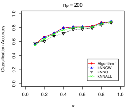
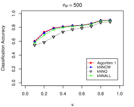
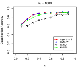
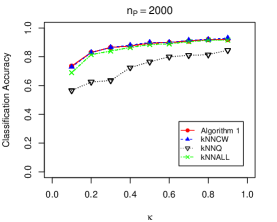
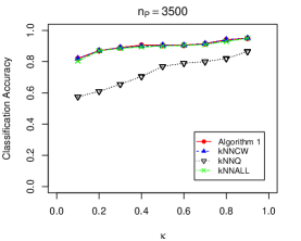
Figure 3: DGP 1 (Smooth Source): Classification accuracy under different combinations of $(n_{P},\kappa)$.

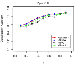
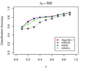
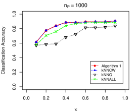
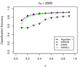
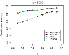
Figure 4: DGP 2 (Smooth Target): Classification accuracy under different combinations of $(n_{P},\kappa)$.

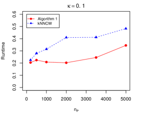
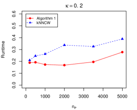
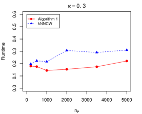
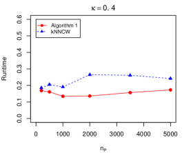
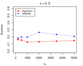
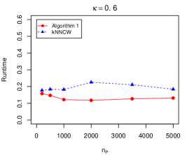
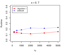
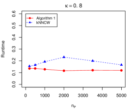
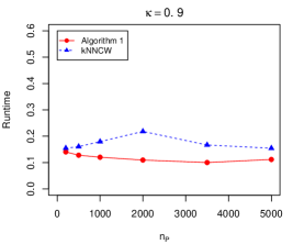
Figure 5: Runtime (in minutes) of Algorithm 1 and kNNCW of DGP 1 under different $(n_{P},\kappa)$.

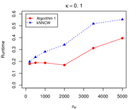
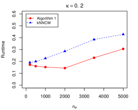
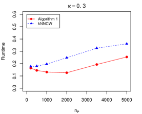
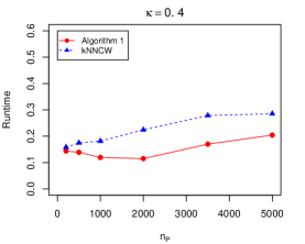
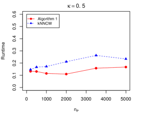
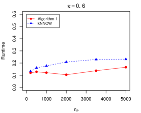
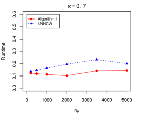
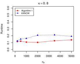
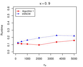
Figure 6: Runtime (in minutes) of Algorithm 1 and kNNCW of DGP 2 under different $(n_{P},\kappa)$.

5 Empirical Application

We apply the proposed adaptive algorithm to the Australian Credit Approval dataset (Quinlan,, 1987) downloaded from UCI machine learning repository (Dua and Graff,, 2017). After removing missing values, we keep four continuous explanatory variables $V_{2},V_{3},V_{7},V_{13}$ and normalize them into $[0,1]$, whose descriptive statistics are summarized in Table 2. The response variable $y\in\{0,1\}$ indicates approval or disapproval status. Based on the binary explanatory variable $V_{1}\in\{0,1\}$, we further divide the observations into two datasets: $P$-data consists of $468$ observations and $Q$-data consists of $222$ observations. We randomly selected $n_{Q}$ observations from $Q$-data with $n_{Q}=100,120,140$, and combined them with $P$-data to train the four classifiers: Algorithm 1, $k$NNCW, $k$NNQ, and $k$NNALL. The rest $222-n_{Q}$ observations are treated as the testing dataset. The classification accuracy is calculated based on $100$ independent replications. Results are summarized in Table 3 which indicate that our proposed algorithm leads to a slightly better classification accuracy.

	$V_{2}$	$V_{3}$	$V_{7}$	$V_{13}$			V1	y
1st Qu.	0.134	0.036	0.006	0.040		class 0	222	383
Median	0.224	0.098	0.035	0.080		class 1	468	307
Mean	0.268	0.170	0.078	0.092
3rd Qu.	0.360	0.257	0.092	0.136

Table 2: Descriptive statistics for the Australian Credit Approval dataset.

$n_{Q}$	Algorithm 1	KNNCW	KNNQ	KNNALL
100	57.52	56.61	52.36	56.16
120	57.33	56.43	52.79	56.01
140	56.53	56.04	53.26	55.72

Table 3: Classification performance of the Australian Credit Approval dataset for different classifiers.

References

- Andrea and Samory, (2017) Andrea, C. A. L. and Samory, K. (2017). Adaptivity to noise parameters in nonparametric active learning. volume 65 of Proceedings of Machine Learning Research, pages 1383–1416, Amsterdam, Netherlands. PMLR.
- Audibert and Tsybakov, (2007) Audibert, J.-Y. and Tsybakov, A. B. (2007). Fast learning rates for plug-in classifiers. The Annals of Statistics, 35(2):608–633.
- Ben-David et al., (2007) Ben-David, S., Blitzer, J., Crammer, K., and Pereira, F. (2007). Analysis of representations for domain adaptation. In Schölkopf, B., Platt, J. C., and Hoffman, T., editors, Advances in Neural Information Processing Systems, pages 137–144. MIT Press.
- Blitzer et al., (2008) Blitzer, J., Crammer, K., Kulesza, A., Pereira, F., and Wortman, J. (2008). Learning bounds for domain adaptation. In Platt, J. C., Koller, D., Singer, Y., and Roweis, S. T., editors, Advances in Neural Information Processing Systems, pages 129–136. Curran Associates, Inc.
- Cai and Wei, (2019) Cai, T. T. and Wei, H. (2019). Transfer learning for nonparametric classification: Minimax rate and adaptive classifier. The Annals of Statistics. To appear.
- Cannings et al., (2020) Cannings, T. I., Fan, Y., and Samworth, R. J. (2020). Classification with imperfect training labels. Biometrika, 107(2):311–330.
- Dua and Graff, (2017) Dua, D. and Graff, C. (2017). UCI machine learning repository.
- Gao et al., (2016) Gao, W., Wang, L., Li, Y.-F., and Zhou, Z.-H. (2016). Risk minimization in the presence of label noise. In AAAI, pages 1575–1581.
- Han et al., (2018) Han, D., Liu, Q., and Fan, W. (2018). A new image classification method using cnn transfer learning and web data augmentation. Expert Systems with Applications, 95:43–56.
- Hanneke and Kpotufe, (2019) Hanneke, S. and Kpotufe, S. (2019). On the value of target data in transfer learning. In Advances in Neural Information Processing Systems, pages 9871–9881.
- Hoffman et al., (2018) Hoffman, J., Mohri, M., and Zhang, N. (2018). Algorithms and theory for multiple-source adaptation. In Advances in Neural Information Processing Systems, pages 8246–8256.
- Huang et al., (2007) Huang, J., Gretton, A., Borgwardt, K., Schölkopf, B., and Smola, A. J. (2007). Correcting sample selection bias by unlabeled data. In Advances in Neural Information Processing Systems, pages 601–608.
- Hussain et al., (2018) Hussain, M., Bird, J. J., and Faria, D. R. (2018). A study on cnn transfer learning for image classification. In UK Workshop on Computational Intelligence, pages 191–202. Springer.
- Kim and Park, (2017) Kim, J. and Park, C. (2017). End-to-end ego lane estimation based on sequential transfer learning for self-driving cars. In Proceedings of the IEEE Conference on Computer Vision and Pattern Recognition (CVPR) Workshops.
- Kpotufe and Martinet, (2018) Kpotufe, S. and Martinet, G. (2018). Marginal singularity, and the benefits of labels in covariate-shift. arXiv preprint arXiv:1803.01833.
- Mammen et al., (1999) Mammen, E., Tsybakov, A. B., et al. (1999). Smooth discrimination analysis. The Annals of Statistics, 27(6):1808–1829.
- Mansour et al., (2012) Mansour, Y., Mohri, M., and Rostamizadeh, A. (2012). Multiple source adaptation and the rényi divergence. arXiv preprint arXiv:1205.2628.
- Manwani and Sastry, (2013) Manwani, N. and Sastry, P. (2013). Noise tolerance under risk minimization. IEEE transactions on cybernetics, 43(3):1146–1151.
- Natarajan et al., (2017) Natarajan, N., Dhillon, I. S., Ravikumar, P., and Tewari, A. (2017). Cost-sensitive learning with noisy labels. The Journal of Machine Learning Research, 18(1):5666–5698.
- Natarajan et al., (2013) Natarajan, N., Dhillon, I. S., Ravikumar, P. K., and Tewari, A. (2013). Learning with noisy labels. In Advances in Neural Information Processing Systems, pages 1196–1204.
- Quinlan, (1987) Quinlan, J. R. (1987). Simplifying decision trees. International journal of man-machine studies, 27(3):221–234.
- Scott, (2019) Scott, C. (2019). A generalized neyman-pearson criterion for optimal domain adaptation. In Algorithmic Learning Theory, pages 738–761.
- Scott et al., (2013) Scott, C., Blanchard, G., and Handy, G. (2013). Classification with asymmetric label noise: Consistency and maximal denoising. In Conference On Learning Theory, pages 489–511.
- Shang and Cheng, (2017) Shang, Z. and Cheng, G. (2017). Computational limits of a distributed algorithm for smoothing spline. The Journal of Machine Learning Research, 18(1):3809–3845.
- Shimodaira, (2000) Shimodaira, H. (2000). Improving predictive inference under covariate shift by weighting the log-likelihood function. Journal of statistical planning and inference, 90(2):227–244.
- Sugiyama et al., (2008) Sugiyama, M., Nakajima, S., Kashima, H., Buenau, P. V., and Kawanabe, M. (2008). Direct importance estimation with model selection and its application to covariate shift adaptation. In Advances in Neural Information Processing Systems, pages 1433–1440.
- Weiss et al., (2016) Weiss, K., Khoshgoftaar, T. M., and Wang, D. (2016). A survey of transfer learning. Journal of Big data, 3(1):9.
- Zhang et al., (2012) Zhang, C., Zhang, L., and Ye, J. (2012). Generalization bounds for domain adaptation. In Advances in Neural Information Processing Systems, pages 3320–3328.
- Zhang et al., (2017) Zhang, Q., Wu, D., Lu, J., Liu, F., and Zhang, G. (2017). A cross-domain recommender system with consistent information transfer. Decision Support Systems, 104:49–63.
- Zhang et al., (2015) Zhang, Y., Duchi, J., and Wainwright, M. (2015). Divide and conquer kernel ridge regression: A distributed algorithm with minimax optimal rates. The Journal of Machine Learning Research, 16(1):3299–3340.
- Zhao et al., (2018) Zhao, H., Zhang, S., Wu, G., Moura, J. M., Costeira, J. P., and Gordon, G. J. (2018). Adversarial multiple source domain adaptation. In Advances in Neural Information Processing Systems, pages 8559–8570.
- Zhao et al., (2013) Zhao, L., Pan, S. J., Xiang, E. W., Zhong, E., Lu, Z., and Yang, Q. (2013). Active transfer learning for cross-system recommendation. In AAAI. Citeseer.
- Zhu et al., (2011) Zhu, Y., Chen, Y., Lu, Z., Pan, S. J., Xue, G.-R., Yu, Y., and Yang, Q. (2011). Heterogeneous transfer learning for image classification. In AAAI, volume 11, pages 1304–1309.