Fine Perceptive GANs for Brain MR Image Super-Resolution in Wavelet Domain

Abstract

Magnetic resonance imaging plays an important role in computer-aided diagnosis and brain exploration. However, limited by hardware, scanning time and cost, it’s challenging to acquire high-resolution (HR) magnetic resonance (MR) image clinically. In this paper, fine perceptive generative adversarial networks (FP-GANs) is proposed to produce HR MR images from low-resolution counterparts. It can cope with the detail insensitive problem of the existing super-resolution model in a divide-and-conquer manner. Specifically, FP-GANs firstly divides an MR image into low-frequency global approximation and high-frequency anatomical texture in wavelet domain. Then each sub-band generative adversarial network (sub-band GAN) conquers the super-resolution procedure of each single sub-band image. Meanwhile, sub-band attention is deployed to tune focus between global and texture information. It can focus on sub-band images instead of feature maps to further enhance the anatomical reconstruction ability of FP-GANs. In addition, inverse discrete wavelet transformation (IDWT) is integrated into model for taking the reconstruction of whole image into account. Experiments on MultiRes_7T dataset demonstrate that FP-GANs outperforms the competing methods quantitatively and qualitatively.

I Introduction

Magnetic resonance imaging (MRI) is a universally used medical imaging technology for auxiliary diagnosis of brain disease and brain function exploration. Compared with Computed Tomography (CT) and Positron Emission Tomography (PET), MRI provides clearer histopathological detail of soft tissue without cancer causing radiation exposure. However, due to physical constraints, MRI takes much longer time to acquire high-resolution (HR) magnetic resonance (MR) image clinically. It may disturb patients and inevitably lead to motion blur in MR image. There are generally two directions to cut down scanning time: 1) Strengthen magnetic field with more advanced equipment. Magnetic field strength has been improved from low-field ($0.2$-$0.5$ Tesla) to ultra-high-field ($\geq 7$ Tesla) for higher signal noise ratio in many researches[1, 2, 3]. However, ultra-high-field MRI requires expensive hardware equipment and bring potential safety risk, which make it difficult to promote. 2) Apply super-resolution (SR) algorithm. SR algorithms have achieved great success to increase the spatial resolution of MR images[4]. Moreover, it has been validated that computational approaches are more cost-effective and efficient for increasing spatial resolution[5].

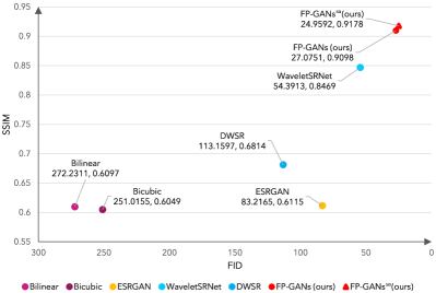
Figure 1: Comparison with different categories of super-resolution methods: interpolation based methods (Bilinear, Bicubic), GAN based method (ESRGAN), wavelet based methods (WaveletSRNet, DWSR) on SSIM and FID metrics. The SSIM and FID values are evaluated on MultiRes_7T dataset with scale factor $\times 4$.

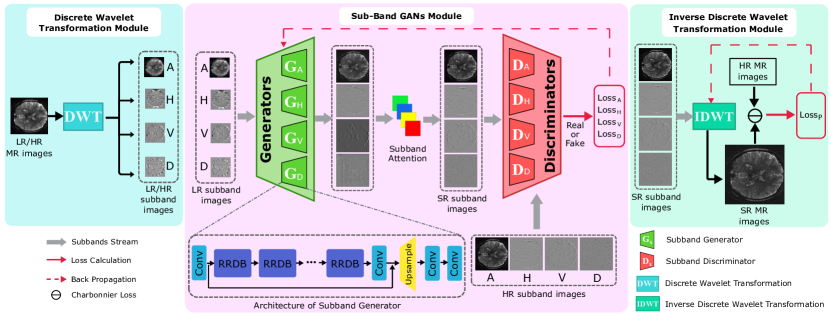
Figure 2: The architecture of FP-GANs. A, H, V and D represent the approximate, vertical, horizontal and diagonal information of MR images respectively. $(G_{A},D_{A}),(G_{H},D_{H}),(G_{V},D_{V}),(G_{D},D_{D})$ are sub-band GANs that learn and predict higher resolution wavelet coefficients.

Since the success of SRCNN[6, 7], single image super-resolution (SISR) has achieved significant improvement qualitatively and quantitatively in recent years. It has attracted lots of interests in MR image super-resolution. For example, Cherukuri[8] enhanced deep MR image super-resolution by a deep network that exploits a low-rank structure and a sharpness prior of MR images. Lyu[9] presented an ensemble learning framework based on multiple GANs, where the complementary priors of five super-resolution algorithms (i.e. ZIP, BI, NEDI, SC and A+) are combined into a GAN model. However, most of existing deep learning based SISR models purely apply CNN for features extraction. It constrains the anatomical detail sensitivity of model and eventually leads to over-smooth result.

In this paper, a novel super-resolution model—fine structure perceptive generative adversarial networks, called fine perceptive GANs (FP-GANs), is designed to alleviate the detail insensitive problem of conventional CNN based models. As shown in Fig. 2, rather than mapping low-resolution MR images to high-resolution counterparts directly, FP-GANs conducts super-resolution in a divide-and-conquer manner with multiple wavelet based generative adversarial networks.

More specifically, one MR image is firstly decomposed into four sub-band images (i.e. LL, LH, HL, HH) in wavelet domain by discrete wavelet transformation (DWT). The four sub-band images represent low-frequency global topology and high-frequency textures respectively. Then, for each sub-band image, a sub-band generative adversarial network (sub-band GAN) is deployed to learn the mapping from LR sub-band image to the corresponding HR sub-band image. With the scheme that learning the distribution of HR sub-bands respectively, it simplifies the mapping task from LR sub-bands to HR sub-bands and thus stabilizes the training procedure of GAN. What’s more, dealing with global topology and detailed texture separately encourage the proposed model to be finer structure sensitive than the traditional deep CNN models. Next, the generated HR sub-band images are weighted by sub-band attention so that the model is able to adjust attention on each sub-band adaptively. Finally, the weighted SR sub-band images are inversely reconstructed into a SR MR image through inverse discrete wavelet transformation (IDWT). IDWT is implemented to be optimizable[10] and hence greatly improves the quality of SR result.

As illustrated in Fig. 1, FP-GANs outperforms the competing models with higher structural similarity index (SSIM)[11] and lower Fréchet Inception Distance (FID)[12]. The main contributions of this paper are summarized as follows:

1) A fine perceptive framework that exploits GANs to process different kinds of texture separately in wavelet domain is proposed. In this manner, it can effectively alleviate the detail insensitive problem. Besides, it simplifies the SR task for a single GAN, which accelerates and stabilizes distribution learning to some extent.

2) Unlike channel attention that trades off attention on feature channels, in this work, sub-band attention is designed to allocate attention on sub-band images adaptively. Extensive experiments demonstrate that sub-band attention contributes to balancing different kinds of textures.

3) Inverse discrete wavelet transformation is implemented optimizable in FP-GANs. It facilitates factoring in the structure of the whole recomposed MR image and hence greatly improves the super-resolution performance.

II Related work

II-A Image Reconstruction in Wavelet Domain

There has been several studies exploring image reconstruction in wavelet domain due to the time-frequency localization of wavelet transformation. For example, Bae[13], Huang[14] and Guo[15] designed a deep convolutional neural network (CNN) to reconstruct high-resolution images with low-resolution wavelet sub-bands for capturing high-frequency textures. However, as the influence of high-frequency textures is relatively small, the textures still would be ignored if the wavelet sub-bands were processed jointly in one CNN model. Liu[16] exploited a multi-level wavelet CNN (MWCNN) to trade off receptive field size and computational efficiency, where wavelet transformation was introduced to reduce the size of feature map. Li[17] proposed a wavelet-domain global and local consistent age generative adversarial network (WaveletGLCA-GAN) to synthesize faces conditioned on age in frequency domain. To achieve better trade-off between objective and perceptual quality, Deng[18] divided the objective quality affected elements from perceptual ones with stationary wavelet decomposition and conquered them separately for different target. Xiao[19] proposed invertible rescaling net (IRN), an invertible bijective transformation based on wavelet transformation, to rescale the down-sampling images losslessly. Zhang[20] utilized wavelet texture loss with the objective to enhance more high-frequency components.

II-B Attention Mechanism

Attention can be defined as a mechanism that allocating more limited available processing resources to more informative components of an object[21]. Recently, attention mechanism (e.g. spatial attention, self attention and channel attention) has been applied to deep neural networks in many studies[22, 23, 24]. Hu[21] proposed squeeze-and-excitation (SE) block to model channel-wise relationships to obtain significant performance improvement for image classification. Wang[25] proposed residual attention network for image classification with a trunk-and-mask attention mechanism. Zhang[23] utilized channel attention mechanism to adaptively rescale channel-wise features maps by considering relevance among channels for highly accurate image super-resolution. Bastidas[26] applied soft attention on individual channels for semantic segmentation.

II-C Network architecture

As shown in Fig. 2, FP-GANs consists of 3 parts in general. Let $I_{LR},I_{HR},I_{SR}$ represent low-resolution, high-resolution and super-resolution MR images respectively. $\left\{LR,HR\right\}$ and $\left\{A,H,V,D\right\}$ are optional list, where A, H, V, D represent the approximation, vertical, horizontal and diagonal texture of magnetic resonance (MR) image respectively. The processing procedure in FP-GANs can be summarized and formulated as follows:

1) Wavelet transformation module. Discrete wavelet transformation (DWT) is applied to decompose MR images into four sub-bands (i.e. LL, LH, HL, HH). These sub-bands contain low-frequency global information and high-frequency texture information in wavelet domain.

$$\begin{split}&I_{A}^{\left\{LR,HR\right\}},I_{H}^{\left\{LR,HR\right\}},I_{V}^{\left\{LR,HR\right\}},I_{D}^{\left\{LR,HR\right\}}\\ =&{\rm{DWT}}\Big{(}I^{\left\{LR,HR\right\}}\Big{)}.\end{split}$$ (1)

2) Sub-band generative adversarial networks module. A group of generative adversarial networks (GANs) take low-resolution sub-band images as input and learn to generate the corresponding high-resolution sub-band images.

$$I_{\left\{A,H,V,D\right\}}^{SR}=G_{\left\{A,H,V,D\right\}}\Big{(}I_{\left\{A,H,V,D\right\}}^{LR}\Big{)}.$$ (2)

Between the generator and discriminator of sub-band GANs, sub-band attention learns to trade off the approximation, horizontal, vertical and diagonal textures of the SR sub-band images. It enhances visual quality by balancing the global topology and detailed textures. The detail of sub-band attention can be found in supplementary material.

$$\Big{[}{I_{A}^{SR}}_{w},{I_{H}^{SR}}_{w},{I_{V}^{SR}}_{w},{I_{D}^{SR}}_{w}\Big{]}=W\cdot\Big{[}I_{A}^{SR},I_{H}^{SR},I_{V}^{SR},I_{D}^{SR}\Big{]}.$$ (3)

3) Inverse wavelet transformation module. Inverse discrete wavelet transformation reconstructs SR MR images by synthesizing the weighted SR sub-band images.

$$I^{SR}={\rm{IDWT}}\Big{(}{I_{A}^{SR}}_{w},{I_{H}^{SR}}_{w},{I_{V}^{SR}}_{w},{I_{D}^{SR}}_{w}\Big{)}.$$ (4)

II-D Discrete wavelet transformation

1-level discrete wavelet transformation (DWT) decomposes an image into four smaller 2D sub-bands: LL (global approximation), LH (horizontal texture), HL (vertical texture), HH (diagonal texture), as Fig. 3a shows. The sub-band images can be losslessly recomposed into the original MR image by inverse discrete wavelet transformation (IDWT) as shown in Fig. 3b.

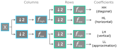
(a)

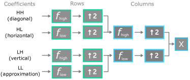
(b)

Figure 3: Procedure of wavelet transformation. (a) 1-level wavelet transformation, decomposing an image into four sub-bands (i.e. LL, LH, HL, HH). (b) 1-level wavelet transformation, recomposing the sub-bands into original image. $f_{high}$ and $f_{low}$ represent high-pass filter and low-pass filter respectively.

Inspired by the lossless recomposition procedure, 1-level 2D DWT is employed in FP-GANs to divide different oriented textures and conquer them. Take Haar based DWT as an example, the transformation instance can be illustrated as Fig. 4.

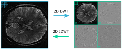
Figure 4: Instance of Haar based discrete wavelet transformation (DWT) and inverse discrete wavelet transformation (IDWT).

Let the filter of Haar based wavelet transformation defined as Equation (5), then the transformation procedure of Fig. 4 can be concisely computed as Equation (6).

$$\begin{split}f_{LL}=\ \begin{bmatrix}\makebox[0.0pt]{1}&\makebox[0.0pt]{1}\\ 1&1\end{bmatrix}\hskip 8.0pt&f_{LH}=\ \begin{bmatrix}-1&-1\\ 1&1\end{bmatrix}\hskip 8.0pt\\ f_{HL}=\ \begin{bmatrix}-1&\makebox[0.0pt]{1}\\ -1&1\end{bmatrix}\hskip 8.0pt&f_{HH}=\ \begin{bmatrix}\makebox[0.0pt]{1}&-1\\ -1&1\end{bmatrix}\hskip 8.0pt\end{split},$$ (5)

$$\begin{cases}a=A+B+C+D\\ b=A+B-C-D\\ c=A-B+C-D\\ d=A-B-C+D\\ \end{cases}\\ \rightleftharpoons\hskip 8.0pt\begin{cases}A=(a+b+c+d)/{4}\\ B=(a+b-c-d)/{4}\\ C=(a-b+c-d)/{4}\\ D=(a-b-c+d)/{4}\\ \end{cases}.$$ (6)

where $A,B,C,D$ represent the pixel intensity in the original MR image in Fig. 4, and $a,b,c,d$ represent the pixel intensity in four sub-bands respectively.

II-E Sub-band GANs

The second part of FP-GANs consists of four pairs of generative adversarial network with same architecture, namely sub-band GANs. Each GAN focuses on one sub-band (i.e. LL, LH, HL, HH), learning to generate higher resolution sub-band images from low-resolution ones. The generators are trained to capture the distribution of HR sub-band images, while the discriminators are encouraged to estimate whether the images are real or generated.

Suppose $X$ denotes low-resolution MR images dataset and Y denotes high-resolution MR images dataset as ground truth. Let $\{x_{i}\}_{i}^{N}\subset X$ and $\{y_{i}\}_{i}^{N}\subset Y$, $N$ denotes the number of MR images. Then the adversarial procedure of traditional super-resolution GAN can be formulated as following min-max problem:

$$\mathop{min}\limits_{G}\mathop{max}\limits_{D}\mathbb{E}_{y\in Y}\Big{[}\log\big{(}D(y)\big{)}\Big{]}+\mathbb{E}_{x\in X}\Big{[}1-\log{\Big{(}D\big{(}G(x)\big{)}\Big{)}}\Big{]}.$$ (7)

Due to the usage of relativistic discrimination regime, the objective function in FP-GANs can be formulated as:

$$\mathop{min}\limits_{G}\mathop{max}\limits_{D}\mathbb{E}_{y\in Y}\Big{[}\log\Big{(}D\big{(}y,G(x)\big{)}\Big{)}\Big{]}+\mathbb{E}_{x\in X}\Big{[}\log\Big{(}1-D\big{(}G(x),y\big{)}\Big{)}\Big{]},$$ (8)

where $D\big{(}y,G(x)\big{)}={\rm sigmoid}\Big{(}\mathcal{D}(y)-\mathbb{E}_{x\in X}\big{[}\mathcal{D}\big{(}G(x)\big{)}\big{]}\Big{)}$, $\mathcal{D}(x)$ denotes the output of discriminator.

II-E1 Generator

As illustrated in Fig. 2, the generator of sub-band GAN consists of 5 parts: first convolutional layer, residual-in-residual-dense-blocks (RRDBs) module (Fig. 5), trunk convolutional layer, upsampling module and final convolutional layer referred as ESRGAN[27] and RFB-ESRGAN[28].

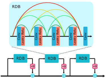
Figure 5: The structure of residual-in-residual-dense-block (RRDB) in generator.

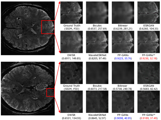
Figure 6: Visual comparison of detail recovery performance on MultiRes_7T dataset. The images are gained with super-resolution scale factor $\times 4$. Red and blue indicate the best and the second best performance, respectively.

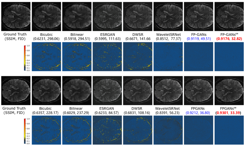
Figure 7: Difference comparison among Bicubic, Bilinear, ESRGAN, DWSR, WaveletSRNet, FP-GANs and FP-GANs^sa with heatmap. Brighter pixel means more difference to the ground truth.

II-F Training Loss

Adversarial loss, wavelet loss and pixel loss are combined to guide the training of FP-GANs from difference perspective.

II-F1 Adversarial Loss

With prior knowledge that real and generated MR images account for a half respectively while supervisedly training, adversarial loss based on relativistic GAN[29] is introduced to stabilize the training and improve the quality of the generated MR image. The adversarial loss function of four sub-band GANs $(G_{A},G_{H},G_{V},G_{D})$ can be defined as:

$$\begin{split}Loss_{D_{\left\{A,H,V,D\right\}}}=&-\mathbb{E}_{y\in Y}\Big{[}\log\big{(}D_{\left\{A,H,V,D\right\}}(y,x_{f})\big{)}\Big{]}\\ &-\mathbb{E}_{x\in X}\Big{[}\log\big{(}1-D_{\left\{A,H,V,D\right\}}(y,x_{f})\big{)}\Big{]},\end{split}$$ (9)

$$\begin{split}Loss_{G_{\left\{A,H,V,D\right\}}}=&-\mathbb{E}_{y\in Y}\Big{[}\log\big{(}1-D_{\left\{A,H,V,D\right\}}(y,x_{f})\big{)}\Big{]}\\ &-\mathbb{E}_{x\in X}\Big{[}\log\big{(}D_{\left\{A,H,V,D\right\}}(y,x_{f})\big{)}\Big{]},\end{split}$$ (10)

where $D(y,x_{f})={\rm sigmoid}\Big{(}\mathcal{D}(y)-\mathbb{E}_{x\in X}\big{[}\mathcal{D}(x_{f})\big{]}\Big{)}$, $\mathcal{D}(x)$ denotes the output of discriminator, $x_{f}=G(x)$, and $\left\{A,H,V,D\right\}$ is an optional list.

II-F2 Wavelet Loss

As textures mainly are comprised of high-frequency components, wavelet loss is introduced for paying more emphasis on high frequency components. The contribution that eliminates over-smooth result and recovers more anatomical detail of MR image will be further demonstrated latter. Wavelet loss on each sub-band can be computed as:

$$\begin{split}&Loss_{W_{\{A,H,V,D\}}}\\ =&\mathbb{E}_{x\in X,y\in Y}\Big{[}\Big{\|}y_{\{A,H,V,D\}}-G_{\{A,V,H,D\}}\big{(}x_{\{A,H,V,D\}}\big{)}\Big{\|}_{1}\Big{]},\end{split}$$ (11)

where $x_{\{A,H,V,D\}}$ and $y_{\{A,H,V,D\}}$ denote the low and high resolution sub-band images, respectively.

II-F3 Pixel Loss

Pixel loss, factoring the global structure of the reconstructed image, is calculated by Charbonnier penalty function as Equation (12). Charbonnier penalty function is a differential variant of $L_{1}$ normalization. It can avoid the over-smooth effect of $L_{2}$ normalization.

$$\begin{split}&Loss_{P}\\ =&\mathbb{E}_{x_{f}\in X,y\in Y}\Bigg{[}\sqrt{\big{(}y-{\rm{IDWT}}(x_{f}^{A},x_{f}^{H},x_{f}^{V},x_{f}^{D})\big{)}^{2}+\epsilon^{2}}\Bigg{]},\end{split}$$ (12)

where $x_{f}^{A},x_{f}^{H},x_{f}^{V},x_{f}^{D}$ represent the sub-band images predicted by $G_{\{A,V,H,D\}}$ respectively. $\epsilon$ is a slack variable and empirically set as $1\times 10^{-6}$.

II-F4 FP-GANs Loss

Overall, the total loss function of generators in FP-GANs can be defined as:

$$\begin{split}Loss_{G_{total}}=&\lambda_{1}Loss_{A}+\lambda_{2}Loss_{H}+\lambda_{3}Loss_{V}+\lambda_{4}Loss_{D}\\ &+\beta Loss_{P},\end{split}$$ (13)

where $Loss_{\{A,H,V,D\}}=\alpha Loss_{G_{\{A,H,V,D\}}}+Loss_{W_{\{A,H,V,D\}}}$, $\alpha$ is weighted value that trades off the adversarial loss and wavelet loss. $\lambda_{1},\lambda_{2},\lambda_{3}$ and $\lambda_{4}$ are parameters that relatively control the penalty on corresponding sub-band and facilitate textures trade-off.

Analogously, the discriminators of FP-GANs can be optimized by minimizing the following function:

$$Loss_{D_{total}}=Loss_{D_{A}}+Loss_{D_{H}}+Loss_{D_{V}}+Loss_{D_{D}}.$$ (14)

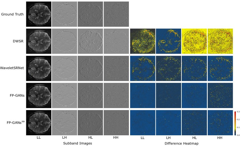
Figure 8: Comparison of sub-band recovery against the wavelet based methods (i.e. DWSR, WaveletSRNet). Brighter pixel means more difference to the ground truth.

TABLE I: Quantitative evaluation for super-resolution performance on MultiRes_7T dataset

Scale		Bicubic	Bilinear	ESRGAN	DWSR	WaveletSRNet	FP-GANs	FP-GANssa
$\times 2$	PSNR	27.4957	27.6820	27.6074	–	24.7976	28.2176	27.8190
	SSIM	0.8269	0.7894	0.8546	–	0.9366	0.9225	0.9226
	FID	104.22	124.53	48.41	–	22.77	25.01	26.01
$\times 4$	PSNR	25.2539	24.8464	21.8490	23.2888	26.6529	25.0345	27.5964
	SSIM	0.6408	0.6097	0.6115	0.6800	0.8469	0.9098	0.9178
	FID	251.01	272.23	83.21	113.16	54.39	27.07	24.95
$\times 8$	PSNR	22.8815	22.7049	17.8975	–	21.7509	20.7491	21.2957
	SSIM	0.4528	0.4412	0.3463	–	0.6595	0.7947	0.8036
	FID	318.74	403.33	98.03	–	83.06	124.71	116.13

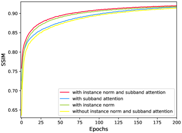
(a)

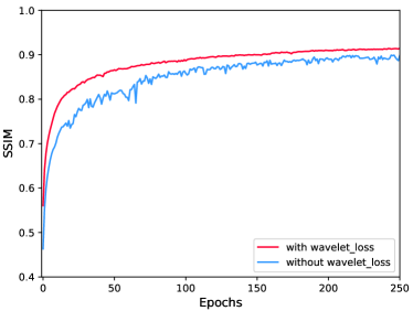
(b)

Figure 9: Ablation study: (a) Ablation study on instance normalization and sub-band attention. (b) Ablation study on wavelet loss.

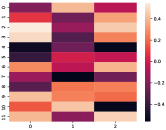
(a) 0th epoch

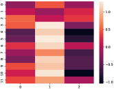
(b) 50th epoch

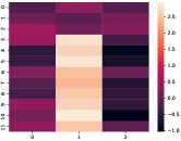
(c) 100th epoch

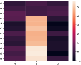
(d) 200th epoch

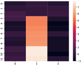
(e) 400th epoch

Figure 10: The weight update procedure of sub-band attention (SA) module. 0-2 rows denote the weight of LL sub-band, and 3-5, 6-8, 9-11 rows denote LH, HL and HH sub-bands respectively. (a) The weight of the initial stage, 0th epoch. (b), (c), (d), (e) are the weight of 50th, 100th, 200th and 400th epoch.

III Experiments

III-A Data preparation

Multi-resolution 7T (MultiRes_7T) functional MR images data was acquired with Siemens 7T scanner from OpenfMRI database with accession number: ds000113c[30]. The dataset consists of ultra high-field functional MR images recorded at four spatial resolutions (0.8 mm, 1.4 mm, 2.0 mm and 3.0 mm isotropic voxel size) from 7 participants.

In the experiment, 0.8 mm and 3.0 mm voxel size functional MR images with shape of $250\times 250\times 57$ and $66\times 66\times 37$ respectively are utilized. Firstly, slice the images into $(250\times 250$ and $66\times 66)$ along z-axis. Secondly, conduct center crop on the slices to cut off redundant content, and get corresponding grayscale images $(200\times 200)$ and $50\times 50)$. Thirdly, downsample the high-resolution images from $200\times 200$ with scale factor (i.e. 2, 4, 8) to acquire corresponding low-resolution images in size $(100\times 100,50\times 50,25\times 25)$ and thus build the paired dataset.

III-B Implementation and Training detail

FP-GANs is implemented with Pytorch and the experiments are conducted on Nvidia Titan RTX. In generator, the number of residual in residual dense block (RRDB) is chosen as 16. In discriminator, there are 10 convolutional layers followed by 2 full connected layers. FP-GANs is optimized with Adam[31]. The batch size is set as 16. The learning rate of the generators is set as $1\times 10^{-4}$ and the learning rate of discriminators is set as $5\times 10^{-4}$. Besides, the learning rate of IDWT is set as $1\times 10^{-4}$. Hyper-parameters $\lambda_{1},\lambda_{2},\lambda_{3},\lambda_{4}$ in Equation (13) are empirically set as $1\times 10^{-1}$. Besides, $\alpha$ and $\beta$ are chosen empirically as $1\times 10^{-4}$ and $1\times 10^{-1}$ respectively.

III-C Evaluation metrics

Peak signal noise ratio (PSNR) and structural similarity index (SSIM) have been commonly applied in many super-resolution researches as standard evaluation metrics. Nevertheless, it was found that high PSNR doesn’t guarantee a high visual quality during experiment. As illustrated in Figure 11, Bicubic and Bilinear rank higher in PSNR, but the result of other methods are visually better from human perspective. Study[32] also claimed that PSNR fails to assess image quality accurately with respect to human visual system. Under this circumstance, Fréchet Inception Distance (FID), calculating the feature distance of two images, is utilized to assess the perceptual quality of SR MR images. In summary, PSNR and SSIM are applied to measure the objective quality of images. FID is utilized to assess the visual quality from human perception.

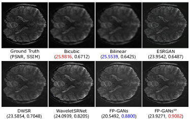
Figure 11: Comparison of quantitative value and visual quality. Red and blue indicate the best and the second best performance, respectively.

III-D Performance

Comprehensive analyses are carried out on MultiRes_7T dataset with super-resolution scale factor $\times 4$. Figure 1 reports the performance of FP-GANs and other competing methods upon SSIM and FID. It can be observed that FP-GANs achieves better both on SSIM and FID value than interpolation based methods (Bicubic and Bilinear), GAN based method (ESRGAN [27]) and wavelet based methods (DWSR [15] and WaveletSRNet [14]). Typically, equipped with sub-band attention, FP-GANs^sa behaves a little better than FP-GANs.

As illustrated in Figure 6, the interpolation based methods produce over-smooth results. GAN based method—ESRGAN reproduces rich textures though, the result loses its coherency with the input. FP-GANs recovers finer anatomical structure with shaper and clearer textures while remaining consistency. To further examine the detail capture ability, difference heatmap, reflecting absolute difference between generated image and corresponding ground truth, is utilized as Figure 7 shows. It can be apparently observed that there is less difference in the heatmap of FP-GANs and FP-GANs^sa than the competing methods. This confirms the detail sensitivity of the proposed structure.

Besides, comparison with wavelet based methods (i.e. DWSR, WaveletSRNet) are conducted to investigate sub-band image reconstruction performance. As shown in Figure 8, sub-band generative adversarial networks (sub-band GANs) of FP-GANs reproduce more authentic sub-band images (LL, LH, HL, HH) in wavelet domain, and thus contributes to produce a compelling super-resolution image.

Table I shows the overview of experiment quantitatively, from which it can be seen that FP-GANs outperforms the competing methods in most case, especially in $\times 4$ case. Moreover, it’s obvious that sub-band attention module exploited in FP-GANs^sa enforces the model handle large scale super-resolution task better. From Figure 9b, it can be concluded that wavelet loss contributes to stabilize and accelerate the convergence of FP-GANs.

IV Ablation Study

From Figure 9a, it can be seen that FP-GANs with instance normalization and sub-band attention mechanism converges most quickly and gets the highest score in SSIM. On the contrary, FP-GANs without the two module performs worst in SSIM. The ablation study on wavelet loss can be seen in Figure 9b. It illustrates that wavelet loss contributes to stabilize and accelerate the convergence of FP-GANs.

Form Figure 10, it can be observed that the weight parameters of sub-band attention gradually update from the initial random distribution to a regular distribution, where more attention are allocated on the high-frequency sub-bands, especially the HH one. This contributes to enhance the high-frequency anatomical textures of MR images.

V Discussion and Conclusion

Losing textures is a universal problem of existing super-resolution methods. In this study, a novel super-resolution model—FP-GANs, integrated with wavelet transformation, is proposed to capture anatomical textures that are mainly in high-frequency. The proposed model divides the MR images into low-frequency and high-frequency sub-bands, and then conquer the super-resolution of each sub-band with a sub-band GAN separately. By treating the low-frequency global topology and high-frequency texture equally during super-resolution stage, it alleviates the detail insensitive problem. On the other hand, it contributes to stabilize training by simplifying the super-resolution task compared to the single GAN method like ESRGAN[27]. Besides, sub-band attention contributes to handle large scale super-resolution. Compared with interpolation and prior deep learning methods, FP-GANs shows its advantage on detail reconstruction, which is most important in medical image field.

References

- [1] R. R. Regatte and M. E. Schweitzer, “Ultra-high-field mri of the musculoskeletal system at 7.0 t,” Journal of Magnetic Resonance Imaging: An Official Journal of the International Society for Magnetic Resonance in Medicine, vol. 25, no. 2, pp. 262–269, 2007.
- [2] M. A. Ertürk, X. Wu, Y. Eryaman, P.-F. Van de Moortele, E. J. Auerbach, R. L. Lagore, L. DelaBarre, J. T. Vaughan, K. Uğurbil, G. Adriany et al., “Toward imaging the body at 10.5 tesla,” Magnetic resonance in medicine, vol. 77, no. 1, pp. 434–443, 2017.
- [3] S. Geethanath and J. T. Vaughan Jr, “Accessible magnetic resonance imaging: A review,” Journal of Magnetic Resonance Imaging, vol. 49, no. 7, pp. e65–e77, 2019.
- [4] E. Van Reeth, I. W. Tham, C. H. Tan, and C. L. Poh, “Super-resolution in magnetic resonance imaging: a review,” Concepts in Magnetic Resonance Part A, vol. 40, no. 6, pp. 306–325, 2012.
- [5] E. Plenge, D. H. Poot, M. Bernsen, G. Kotek, G. Houston, P. Wielopolski, L. van der Weerd, W. J. Niessen, and E. Meijering, “Super-resolution methods in mri: can they improve the trade-off between resolution, signal-to-noise ratio, and acquisition time?” Magnetic resonance in medicine, vol. 68, no. 6, pp. 1983–1993, 2012.
- [6] C. Dong, C. C. Loy, K. He, and X. Tang, “Learning a deep convolutional network for image super-resolution,” in European conference on computer vision. Springer, 2014, pp. 184–199.
- [7] ——, “Image super-resolution using deep convolutional networks,” IEEE transactions on pattern analysis and machine intelligence, vol. 38, no. 2, pp. 295–307, 2015.
- [8] V. Cherukuri, T. Guo, S. J. Schiff, and V. Monga, “Deep mr brain image super-resolution using spatio-structural priors,” IEEE Transactions on Image Processing, vol. 29, pp. 1368–1383, 2019.
- [9] Q. Lyu, H. Shan, and G. Wang, “Mri super-resolution with ensemble learning and complementary priors,” IEEE Transactions on Computational Imaging, vol. 6, pp. 615–624, 2020.
- [10] F. Cotter and N. Kingsbury, “A learnable scatternet: Locally invariant convolutional layers,” in 2019 IEEE International Conference on Image Processing (ICIP). IEEE, 2019, pp. 350–354.
- [11] Z. Wang, A. C. Bovik, H. R. Sheikh, and E. P. Simoncelli, “Image quality assessment: from error visibility to structural similarity,” IEEE transactions on image processing, vol. 13, no. 4, pp. 600–612, 2004.
- [12] D. Dowson and B. Landau, “The fréchet distance between multivariate normal distributions,” Journal of Multivariate Analysis, vol. 12, no. 3, pp. 450 – 455, 1982. [Online]. Available: http://www.sciencedirect.com/science/article/pii/0047259X8290077X
- [13] W. Bae, J. Yoo, and J. Chul Ye, “Beyond deep residual learning for image restoration: Persistent homology-guided manifold simplification,” in Proceedings of the IEEE conference on computer vision and pattern recognition workshops, 2017, pp. 145–153.
- [14] H. Huang, R. He, Z. Sun, and T. Tan, “Wavelet-srnet: A wavelet-based cnn for multi-scale face super resolution,” in Proceedings of the IEEE International Conference on Computer Vision, 2017, pp. 1689–1697.
- [15] T. Guo, H. Seyed Mousavi, T. Huu Vu, and V. Monga, “Deep wavelet prediction for image super-resolution,” in Proceedings of the IEEE Conference on Computer Vision and Pattern Recognition Workshops, 2017, pp. 104–113.
- [16] P. Liu, H. Zhang, K. Zhang, L. Lin, and W. Zuo, “Multi-level wavelet-cnn for image restoration,” in Proceedings of the IEEE Conference on Computer Vision and Pattern Recognition Workshops, 2018, pp. 773–782.
- [17] P. Li, Y. Hu, R. He, and Z. Sun, “Global and local consistent wavelet-domain age synthesis,” IEEE Transactions on Information Forensics and Security, vol. 14, no. 11, pp. 2943–2957, 2019.
- [18] X. Deng, R. Yang, M. Xu, and P. L. Dragotti, “Wavelet domain style transfer for an effective perception-distortion tradeoff in single image super-resolution,” in Proceedings of the IEEE International Conference on Computer Vision, 2019, pp. 3076–3085.
- [19] M. Xiao, S. Zheng, C. Liu, Y. Wang, D. He, G. Ke, J. Bian, Z. Lin, and T.-Y. Liu, “Invertible image rescaling,” in Proceedings of the European Conference on Computer Vision (ECCV), 2020.
- [20] Y. Zhang, Z. Zhang, S. DiVerdi, Z. Wang, J. Echevarria, and Y. Fu, “Texture hallucination for large-factor painting super-resolution,” in Proceedings of the European Conference on Computer Vision (ECCV), 2020.
- [21] J. Hu, L. Shen, and G. Sun, “Squeeze-and-excitation networks,” in Proceedings of the IEEE conference on computer vision and pattern recognition, 2018, pp. 7132–7141.
- [22] L. Chen, H. Zhang, J. Xiao, L. Nie, J. Shao, W. Liu, and T.-S. Chua, “Sca-cnn: Spatial and channel-wise attention in convolutional networks for image captioning,” in Proceedings of the IEEE conference on computer vision and pattern recognition, 2017, pp. 5659–5667.
- [23] Y. Zhang, K. Li, K. Li, L. Wang, B. Zhong, and Y. Fu, “Image super-resolution using very deep residual channel attention networks,” in Proceedings of the European Conference on Computer Vision (ECCV), 2018, pp. 286–301.
- [24] K. Li, Z. Wu, K.-C. Peng, J. Ernst, and Y. Fu, “Tell me where to look: Guided attention inference network,” in Proceedings of the IEEE Conference on Computer Vision and Pattern Recognition, 2018, pp. 9215–9223.
- [25] F. Wang, M. Jiang, C. Qian, S. Yang, C. Li, H. Zhang, X. Wang, and X. Tang, “Residual attention network for image classification,” in Proceedings of the IEEE Conference on Computer Vision and Pattern Recognition, 2017, pp. 3156–3164.
- [26] A. A. Bastidas and H. Tang, “Channel attention networks,” in Proceedings of the IEEE Conference on Computer Vision and Pattern Recognition Workshops, 2019, pp. 0–0.
- [27] X. Wang, K. Yu, S. Wu, J. Gu, Y. Liu, C. Dong, Y. Qiao, and C. Change Loy, “Esrgan: Enhanced super-resolution generative adversarial networks,” in Proceedings of the European Conference on Computer Vision (ECCV), 2018, pp. 0–0.
- [28] K. Zhang, S. Gu, and R. Timofte, “Ntire 2020 challenge on perceptual extreme super-resolution: Methods and results,” in Proceedings of the IEEE/CVF Conference on Computer Vision and Pattern Recognition Workshops, 2020, pp. 492–493.
- [29] A. Jolicoeur-Martineau, “The relativistic discriminator: a key element missing from standard gan,” arXiv preprint arXiv:1807.00734, 2018.
- [30] A. Sengupta, R. Yakupov, O. Speck, S. Pollmann, and M. Hanke, “Ultra high-field (7 t) multi-resolution fmri data for orientation decoding in visual cortex,” Data in brief, vol. 13, pp. 219–222, 2017.
- [31] D. P. Kingma and J. Ba, “Adam: A method for stochastic optimization,” in 3rd international conference for learning representations, San Diego, 2015.
- [32] C. Ledig, L. Theis, F. Huszár, J. Caballero, A. Cunningham, A. Acosta, A. Aitken, A. Tejani, J. Totz, Z. Wang et al., “Photo-realistic single image super-resolution using a generative adversarial network,” in Proceedings of the IEEE conference on computer vision and pattern recognition, 2017, pp. 4681–4690.