Characterization of Folding and Stretching in Mixing Enhancements

Abstract

This research paper presents a 2D numerical model of an electrokinetic T-junction micro-mixer based on the stretching and folding theory presented by Ottino. Particle deformation was considered by simulating 2 $\mu m$ massless particles as 8-point square cells. Furthermore, stretching and folding definitions are proposed, compatible with a Lagrangian particle approach. Moreover, mixing homogeneity and consistency were measured in a 200 $\mu m$ square region of interest neighboring the outlet. Statistical analysis of the exiting mixing homogeneity at four different electric field conditions (93.5 $V/cm$, 109.8 $V/cm$, 126 $V/cm$ and 117.9 $V/cm$, corresponding to a 23$V$, 27$V$, 29$V$ and 31V potential difference) show that mixing consistency and homogeneity are not always increased with a higher electric field intensity, even after electrokinetic instabilities are formed, as increasingly unstable flow conditions decrease the ratio of folding to stretching ($m$), hindering the interaction between substances. Finally, an optimal proportion of stretching to folding was found for maximizing mixing efficiency at $m=0.0045$.

I Introduction

Over the past 20 years there has been extensive research going into reducing the time and cost for chemical analysis and pathogen detection. Particularly, development of chip devices for micro total analysis systems ($\mu$TAS) has been on the rise. These systems are often composed of a series of microchannels to operate, and as such, the study of small-scale channel flows has led the way for various areas of study; one of them being electrokinetic (EK) flow. EK flow is a type of flow which is driven by an electric field Gill (1990). In terms of physical variables, this field studies the coupling of fluid flow, electric fields and the transport of species. In the past, because of the scale of these $\mu$TAS apparatus, achieving high Reynolds numbers by using pressure gradients, to induce turbulence and catalyze chemical reactions, proved to be a challenge, as mixing of species would occur primarily by diffusion. Diffusion is not a hasty process, and as such, mixing channel sizes were constrained to be larger. As a result, several designs were created to ameliorate the mixing of species inside by modifying the geometries Wang and Hu (2010); Stroock et al. (2002); Bakker, Laroche, and Marshall (2000), however, thanks to the study of EK flows, it was soon proved that turbulence can be induced in laminar flows Wang, Yang, and Zhao (2014), in the form of electrokinetic instabilities (EKI), allowing for smaller and more efficient micromixers. The study of EKI formation and the determination of parameters, such as the electrical Rayleigh number $Ra_{e}$ Chen et al. (2005); Baygents and Baldessari (1998); Lin et al. (2004) to ensure reproducibility of this newfound turbulence would pave the way for new sophisticated micromixer setups. From pulsating electric field ideas Glasgow, Batton, and Aubry (2004); Kang, Heo, and Suh (2008) to diverse geometries Azimi, Nazari, and Daghighi (2017); Posner and Santiago (2006); Li, Delorme, and Frankel (2016) including herringbone passive mixers Stroock et al. (2002); Camesasca, Kaufman, and Manas-Zloczower (2006); Aubin et al. (2003), several steps were taken to improve mixture homogeneity. Theory wise, important advances on chaotic mixing theoryBaker, Gollub, and Fox (1990); Ottino (1989) were made, particularly describing the mixing process as a series of transformations that the fluid undergoes by stretching and folding until a homogenous product is achieved.

In the present, significant contributions have been made on the further study of stretching and its mixing enhancements Kelley and Ouellette (2011); Voth, Haller, and Gollub (2002); Arratia, Voth, and Gollub (2005), yet, there is still a lack of consensus on how both of these deformation processes (stretching and folding) impact directly, the mixing homogeneity in EK flows. In this investigation, a 2D T-junction geometry is studied via Finite Element Method (FEM) simulations and a relationship between folding, stretching and mixing quality is found. Moreover, a validated model is proposed, compatible with a Lagrangian particle approach. Mixing consistency through time is measured using statistical methods, by analyzing a region of interest neighboring the outlet of the microchannel. Finally, voltage is related to stretching and folding and their rate of change in the short term.

II Methods and materials

II.1 Folding and Stretching

In this work we investigate the role of stretching and folding and their influence in flow mixing. A series of 2D simulations were carried out using the FEM, to study their effect in a T - shaped microchannel. Based on Ottino’s Ottino (1989) theory of stretching and folding, mixing was characterized by the reduction of curvilinear fluid filament length scales. Adapting this general proposition to a Lagrangian, particle simulation, gives rise to practical definitions for studying both mechanisms in a two-dimensional domain.

Originally, stretching ($\lambda$) was defined by Ottino Ottino (1989) as the deformation of an infinitesimal fluid length, i.e.,

$$\lambda=\lim_{|d\mathbf{X}|\to 0}\frac{d\mathbf{x}}{d\mathbf{X}}.$$ (1)

Where, $|d\mathbf{X}|$ is the magnitude of the initial stretch vector at initial time $t_{0}=0$ and $|d\mathbf{x}|$ is the magnitude of the stretch vector at time $t$. Adapting this definition to a discrete particle approach, it follows that,

$$S_{1j}=\left(\frac{\Delta s_{1}}{s_{1}}\right)_{j},$$ (2)

$$S_{2j}=\left(\frac{\Delta s_{2}}{s_{2}}\right)_{j},$$ (3)

where $S_{1_{j}}$ and $S_{2_{j}}$ represent the stretching of the initial lengths $s_{1}$ and $s_{2}$ shown on Fig. 1. The subscript $j$ is referent to the cell $j$.

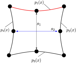
Figure 1: Diagram of eight-point massless cell subjected to stretching and folding.

Figure 1 shows the massless cell, composed by eight points, used to evaluate stretching and folding. Where $P_{i}(x),(i=1,2,3,4)$ are the best-fit, second order polynomial functions that join the points on each of the four sides of the cell and x is the streamwise direction.

The principal stretching direction out of $s_{1}$ and $s_{2}$, for each cell is defined using Eq. (4) as,

$$S_{j}=\max(S_{1j},S_{2j}).$$ (4)

The stretching average value for both directions for all massless cells analyzed, is calculated by Eq. (5) as,

$$\bar{S}=\frac{1}{N}\sum_{j}^{N}S_{j}.$$ (5)

where $N$ is the total number of analyzed cells, at a given time.

Analogously, the folding can be interpreted as the bending deformation of the cell $\varepsilon$, derived from the Euler - Bernoulli beam theory, shown by Hibbeler, (2010) Hibbeler (2010) in Eq. (6).

$$\varepsilon=\frac{-y}{R}=-\kappa y,$$ (6)

where $R$ is the curvature radius, $y$ is the distance from the neutral axis and $\kappa$ is the curvature. When the distance y is shorter than 2 $\mu m$, Eq. (6) can be simplified and rewritten as Eq. (7).

$$\varepsilon=\pm\frac{1\mu m}{R}=\pm\kappa y.$$ (7)

Since the direction of the bending or folding of the cell is irrelevant for the purposes of fluid mixing, we propose a new general definition which must be applicable to all discrete cells in the simulated flow. Based on the mathematical definition of curvature for one-dimensional functions Stewart (2010), the curvature for each side of the cell can be expressed by Eq. (8).

$$k_{i}=\frac{|p_{i}^{\prime\prime}(x)|}{\left(1+p_{i}^{\prime}(x)^{2}\right)^{\frac{3}{2}}}\Bigg{\rvert}_{x=x_{2}}$$ (8)

where $p_{i}^{\prime\prime}(x)$ is the second derivative and $p_{i}^{\prime}$ (x) is the first derivative of $p_{i}(x)$ with respect to the variable $x$, respectively. Moreover, $x_{2}$ is the mid-point of the side $i$. Given $k_{i}$, which corresponds to the curvature of one side of the cell, then the maximum curvature of the cell can be determined using Eq. (9).

$$K_{j}=\max(k_{1},k_{2},k_{3},k_{4})$$ (9)

Where the subscript $j$ refers to the cell that is being analyzed at a given time. The complete folding process is characterized by averaging the $K_{j}$ values over N cells at a given time given by Eq. (10):

$$\bar{F}=\frac{1}{N}\sum_{j}^{N}K_{j}$$ (10)

The total average deformation, that considers the folding (bending) and stretching effects is defined as the sum of both, see Eq. (11).

$$\nu=\bar{S}+\bar{F}$$ (11)

II.2 Mixing index

To correlate the quality of the mixer to the stretching and folding. The following mixing index expression, previously defined by other authors Bakker, Laroche, and Marshall (2000); Kang, Heo, and Suh (2008); Wu and Liu (2003); Lu, Ryu, and Liu (2001); Jayaraj, Kang, and Suh (2007) will be employed to evaluate quantitatively the homogeneity of the mixture.

$$D=\sqrt{\frac{1}{N}\sum_{k,l}^{N}\left(1-\frac{c_{k,l}}{\bar{c}}\right)}$$ (12)

Where $c_{k,l}$ is the concentration of the node $(k,l)$, $\bar{c}$ is the spatial average of concentration for the whole fluid domain, and $N$ is the total number of data points in the sample. $D$ then indicates the coefficient of variation, CoV, of the spatial concentration. As $D$ decreases, the mixture concentration deviates less from the mean, becoming more homogeneous.

Defining mixing efficiency, as a quantity that increases proportionally with mixture homogeneity, is more intuitive and therefore, defined by Eq. (13) as,

$$\text{Mixing efficiency}=100\cdot(1-D)$$ (13)

The focus of this paper is based on the mixture leaving the microchannel, hence, a 200 $\mu m$ box neighboring the outlet, pictured in Figure 2, was designated as the interest region to study the D value. This way, the whole width of the microchannel is considered while the effects of upstream turbulence are dampened, so that only EKI affect the $D$ values.

II.3 Numerical Simulation

A 2D electrokinetic flow was simulated in a T-junction microchannel, using the finite element method (FEM). A time-dependent approach was used, for varying simulated time spans, considering the simulation time is double than the characteristic time $t^{*}=\frac{|\mathbf{V}|}{L_{T}}$ Kang et al. (2006)¸ with $L_{T}$ the distance from the inlet to the outlet of the microchannel and $\mathbf{V}$ the flow average velocity. In order to effectively create chaotic motion, a series of simulations with a range of increasing electric potential $\phi$ were carried out to find the most suitable conditions for flow instabilities (EKI). Additionally, all simulations were carried out for constant values of the conductivity ratio $\gamma=\frac{\sigma_{H}}{\sigma_{L}}$ and zeta potential $\zeta$. Table 1 shows the fluid properties considered in our study.

Table 1: Fluid Properties used for the numerical simulation.

$\rho$	$D_{eff}$	$\mu$	$\zeta$	$\varepsilon$	$\sigma_{H}$	$\sigma_{L}$
1000 $\frac{kg}{m3}$	1.989$\cdot 10^{9}\frac{m^{2}}{s}$	0.001 $Pa\cdot s$	-0.088 V	6.933 $\cdot 10^{-10}\frac{F}{m}$	0.15 $\frac{S}{m}$	0.01 $\frac{S}{m}$

In this analysis, the governing equations of mass conservation for an incompressible and Newtonian fluid (Eq. (14)), momentum balance (including the electrical driving force) (Eq. (15)), electric current conservation (Eq. (16)) and species conservation (Eq. (17)) are solved simultaneously.

$$\nabla\cdot\mathbf{V}=0$$ (14)

$$\rho\left(\frac{\partial\mathbf{V}}{\partial t}+\mathbf{V}\cdot(\nabla\mathbf{V})\right)=-\nabla p+\mu\nabla^{2}\mathbf{V}+\rho_{f}\mathbf{E}$$ (15)

$$\frac{\partial\rho_{e}}{\partial t}+\nabla\cdot\mathbf{J}=0$$ (16)

$$\frac{\partial C}{\partial t}+\mathbf{V}\cdot(\nabla C)=\nabla\cdot(D_{eff}\nabla C)$$ (17)

For Eqs. (14) and (15), $\mathbf{V}$ is the velocity field, $p$ is the pressure field, $\rho$ is the density of the fluid, $\mu$ is the dynamic viscosity of the fluid and $\mathbf{E}$ is the electric field. The charge density $\rho_{f}$ is defined by Gauss’ Law Gill (1990) as $\rho_{f}=\varepsilon\nabla\cdot\mathbf{E}$, where $\mathbf{E}$ itself is defined by $\mathbf{E}=-\nabla\phi$ and the permittivity is defined as $\varepsilon=\varepsilon_{r}\varepsilon_{0}$. Where $\varepsilon_{r}$ and $\varepsilon_{0}$ are the dielectric constant for water and universal permittivity, respectively. In Eq. 16, $\rho_{e}$ is the electric current density, $\mathbf{J}$ is the total electrical current of the system, $C$ is the species concentration and $D_{\text{eff}}$ is the effective diffusivity, given by Posner and Santiago (2006); Luo (2009):

$$D_{\text{eff}}=\frac{2D_{+}+D_{-}}{D_{+}+D_{-}}.$$ (18)

Where $D_{\pm}$ is the cationic/anionic diffusivity coefficient, defined as $D_{\pm}=RTm_{\pm}$. Parameter $R$ is the universal gas constant, $T$ is the absolute temperature and $m_{\pm}$ is the ionic mobility.

In order to solve the PDE system of Eqs. (14) – (17), a highly non-linear Newton-Raphson solver was used, with a minimum dampening factor of 0.0001. To characterize the EKI the electrical Rayleigh number $Ra_{e}=\frac{\varepsilon E^{2}\frac{d}{2}}{\mu D}$ defined by Hao et al. (2004) Lin et al. (2004) was used. Where EKI form only after a certain critical electrical Rayleigh number $Ra_{e_{cr}}$ has been reached. Once the velocity field was determined, the particle trajectories were calculated by solving the kinematics $\frac{d\vec{q}}{dt}=\mathbf{V}$ by the Lagrangian approach, using a constant Newton-Raphson method.

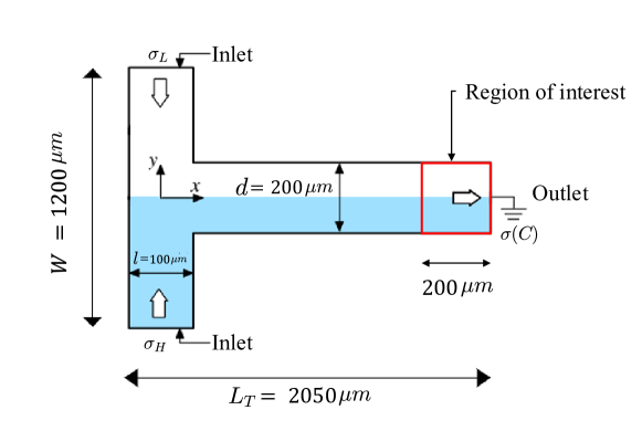
Figure 2: 2D Computational domain for the numerical model, where the blue area represents a high conductivity fluid and the white area represents a low conductivity one. The red box encloses the domain where mixing will be investigated.

Figure 2 shows the T-junction computational domain that was simulated, along with its dimensions. These include: the distance between the upper and lower inlets $W=1200$ $\mu m$, the microchannel outlet and inlet widths $d=200\mu m$ and $l=100\mu m$, respectively, and the microchannel total length $L_{T}=2050\mu m$. The lower inlet allowed flow of high electric conductivity $\sigma_{H}$ fluid while the upper inlet allowed low electric conductivity $\sigma_{L}$ fluid into the domain. We propose Eq. II.3 in order to take into account the temporal and spatial variation of the electrical conductivity $\sigma$ which may occur during the mixing process of two miscible fluids with different concentrations $C$.

$$\sigma(C)=\sigma_{H}\bigg{(}\frac{C}{C_{ref}}\bigg{)}+\sigma_{L}\bigg{(}1-\frac{C}{C_{ref}}\bigg{)},$$ (19)

$$\centering C_{ref}\equiv 1;\begin{cases}\text{if}&\text{$C=1\rightarrow\sigma=\sigma_{H}$}\\ \text{if}&\text{ $C=1\rightarrow\sigma=\sigma_{L}$}\\ if&\text{ $0<C<1\rightarrow\sigma_{H}<\sigma<\sigma_{L}$}\end{cases}\@add@centering$$

The following boundary conditions were implemented. For species conservation, a constant concentration $C=0\frac{mol}{m^{3}}$ and $C=1\frac{mol}{m^{3}}$ was set up in the upper and lower inlet respectively. For the momentum conservation equation, a value of 0 $Pa$ was considered for the inlet and outlet pressure, respectively. Finally, for the current conservation equation, the outlet voltage condition was $\phi_{out}=0\text{V}$ and for both inlets equal voltage values were set $\phi_{in_{1}}=\phi_{in_{2}}$ for each of the cases studied, which varied inlet voltage from 23V to 31V. Additionally, the wall boundary conditions considered were: no flow, electroosmotic slip velocity and electrically isolated for the three conservation laws respectively.

To generate the deformable massless cells in space, we released a grid arrangement of 96 particles from each inlet. Each deformable cell was composed by eight particles, in order to mimic a 2 $\mu m$ diameter massless cell as shown in Figure 1. The particle conditions used in the Particle Tracing module include: the particle type, which was set to liquid and massless, the particle dynamic viscosity $\mu_{p}$ and particle surface tension $\sigma_{p}$ values, which were 1 mPa $\cdot$ s and 0.0729 N/m respectively. The particle charge value was Z = 0, neglecting the charge interactions.

III Results and Discussion

III.1 Model Validation

The numerical model’s EKI behavior was proved identical to the literature, as shown in Figure 3.

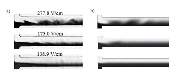
Figure 3: Interfacial behavior comparison for: (a) (0.2 $\times$ EMG 408) and water co-flow in a 45 $\mu m$ deep T-shaped microchannel. High conductivity ferrofluid in black and water in white. Experimental data from Song et al. 2017 Song et al. (2017). (b) 109.8 V/cm simulated flow. High conductivity solution in black and low conductivity solution in white.

Proving similarity to this particular set of experimental results by Song et al. 2017 Song et al. (2017) is significant, as the dimensions of the setup closely match those used in this study. The compared flows were observed on a T-junction setup with dimensions of length $L_{T}$=2000 $\mu m$, distance between the upper and lower inlets $W=700$ $\mu m$ and outlet and inlet widths $d=200$ $\mu m$ and $l=100$ $\mu m$.

Figure 4 shows the mixing efficiency obtained in 29V flow during $t=5.2s$, compared to the normalized results reported by Luo et al. 2008 Winjet et al. (2008). There is a close resemblance in trends, as the average value for the simulated results is of 62% mixing efficiency whereas Luo et al. 2008’s results show 50% mixing efficiency. As both position and time affect the mixing efficiency, finding a similarity in behavior from two different flows, at different times is substantial, as the geometry analyzed by Luo et al. 2008 is comparable to the computational domain used for simulations. The T-junction setup used in the literature had dimensions of length $L_{T}$=1005 $\mu m$, distance between the upper and lower inlets $W=708$ $\mu m$ and outlet and inlet widths $d=60$ $\mu m$ and $l=60$ $\mu m$, respectively.

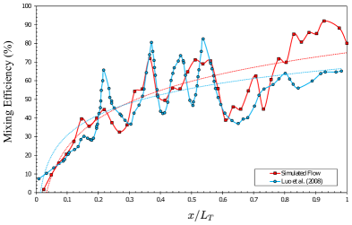
Figure 4: Evolution of mixing efficiency through dimensionless space. 40 datapoints from $x=0$ $\mu m$ to $x=2050$ $\mu m$ are shown in red for a 29V simulated flow at $t=5.2s$. Normalized results from Luo et al. 2008 Winjet et al. (2008), for a 750 V/cm flow at $t=0.3s$ are shown in blue.

III.2 Importance of total deformation in mixing efficiency

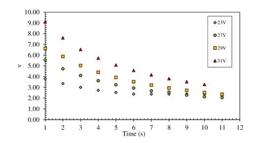
Figure 5: Evolution of $\nu$ with time for 23V, 27V, 29V and 31V flows. 11 timesteps were simulated. Each timestep size was set to 1s.

Figure 5 shows the change in total deformation ($\nu$) with time, for four different voltage conditions. As voltage increases, $\nu$ increases as well, generating a steeper curve that flattens as voltage is decreased. For all flows, it is evident that regardless of the voltage, $\nu$ decreases with time. For lower voltage flows, however, the rate of change of the total deformation is smaller than for the higher voltage flows. Horizontality of the results can be measured by the total deformation change $\Delta\nu$ in the timeframe analyzed. A higher $\Delta\nu$ value represents less horizontality. For instance, for the 31V flow a $\Delta\nu$ value of 5.83 was calculated, the 29V flow showed a $\Delta\nu$ value of 4.26 and the 27V flow’s $\Delta\nu$ was measured at 3.50, whereas the 23V flow, in the same timeframe, had a change in its total deformation of 1.48; plateauing earlier than the other flows, after 6 timesteps. As the voltage across the geometry decreases, EKI dampen, $\nu(t)$ becomes more horizontal and the flow stabilizes in a smaller time window.

To determine if statistically there is an impact in the consistency of the mixture at higher voltages, 50 datapoints were extracted for each of the flows that showed EKI.

Table 2: D Value Intervals for 23V, 27V, 29V and 31V flows.

Voltage	Intervals
	1 [$a=0<b$]	2 [$a-b$]	3 [$a-b$]	4 [$a-b$]	5 [$a-b$]	6 [$a>b=0$]
23V	<0.291	0.291 - 0.320	0.320 - 0.349	0.349 - 0.379	0.379 - 0.408	>0.408
27V	<0.123	0.123 - 0.198	0.198 - 0.273	0.273 - 0.349	0.349 - 0.424	>0.424
29V	<0.000*	0.000 - 0.112*	0.112 - 0.231	0.231 - 0.350	0.350 - 0.469	>0.469
31V	<0.063	0.063 - 0.151	0.151 - 0.238	0.238 - 0.326	0.326 - 0.413	>0.413

Table 2 shows the intervals chosen for the statistical analysis shown in Figure 6, where $a$ is the lower bound and $b$ is the upper bound of each interval, respectively. Intervals 1 - 6 were evenly spaced by one standard deviation. Note that in the case of the 29V flow, the last two intervals reach the minimum value for $D$. This happens because the average $D$ value of the 50 datapoints analyzed for this flow was very small in relation to its standard deviation, and as so, the last intervals fell out of range.

Figure 6 shows four histograms relating the frequency of the mixing value $D$ for the intervals previously defined. From first to sixth, these intervals go from the lowest $D$ value (most homogeneous mixture) to highest. Each graph is presented with its normal trend in red. As the potential difference across the channel increases, the $D$ value distribution begins to shift to the left, decreasing deviation from the average concentration and thus, improving the mixing efficiency. This is evidenced in (a) by the consistent, yet, heterogeneous mixture of the stable 23V flow, as $D$ was found in the range of [0.349 - 0.379] on 72% of the cases. As EKI are generated in (b), the 27V flow shows an increase in mixture homogeneity and a decrease in consistency, as the sample is more evenly distributed along the intervals. As the flow continues to grow unstable, the 29V flow in (c) reaches peak consistency, concentrating 54% of the sample in the third interval and 62% of it in the second and third intervals. As the first three intervals now hold the highest frequency, the homogeneity of the mixture has been improved, producing a consistent $D$ value in the range of [0.000 - 0.231]. The 31V flow in (d), closely follows the consistency and homogeneity obtained in (c) by concentrating 58% of the sample on the first three intervals, corresponding to the $D$ value range of [<0.0631 - 0.238].

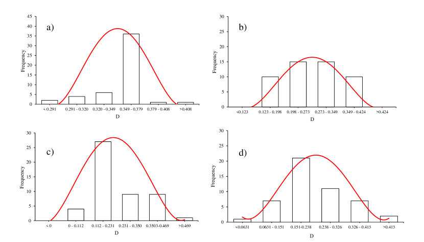
Figure 6: Effect of potential difference on mixing efficiency frequency distribution for (a) 23V where no EKI were formed, (b) 27V EKI present, (c) 29V and (d) 31V. 50 different datapoints were taken for each histogram. The timestep difference between each datapoint was 0.2s.

As higher voltages are studied $\nu$ increases as reported in Figure 5. However, the 31V displayed the highest value for $\nu$, but it did not have the most consistent mixture through time. This shows that further increasing $\nu$ in the microchannel, after 29V does not improve mixing consistency.

Figure 7 shows the relationship between $\bar{S}$ and $\bar{F}$ for three different flow conditions. As established in Figure 5, all flows stabilize with time in terms of $\nu$, and the same holds true in Figure 7, where as time passes, the datapoints decrease in terms of both $\bar{S}$ and $\bar{F}$. To ensure fully developed flow, out of the total simulated time of 11 seconds, only the last 5 seconds were plotted for this analysis. Moreover, to precisely measure the proportional change of $\bar{F}$ in relation to $\bar{S}$, the slope $m$ was defined by Eq. 20,

$$m=\frac{\bar{F}}{\bar{S}}$$ (20)

A stable 23V flow is depicted in Figure 7, which plateaus at a stretching value $\bar{S}$ of 2.376 while showing a pronounced proportion of folding to stretching of $m\to\infty$. As time passes, only folding increases in a stable flow, and therefore $\nu$ varies insignificantly.

Figure 7: Effect of potential difference on proportion between $\bar{F}$ and $\bar{S}$. 23V (square), 29V (dot) and 31V (triangle) flows were analyzed. 25 datapoints were studied per flow. Each datapoint represents a different time and the timestep was set to 0.2s.

After EKI are reached at 27V, further increasing the voltage to 29V displaces the datapoints to another trendline, with a slope $m$ of 0.0043. When comparing the trend of the 31V results to the ones obtained from the 29V flow, it can be observed that the main difference in particle deformation is the proportion of folding to stretching $m$, as the 31V flow always holds a higher value of $\nu$ for every time period analyzed (established in Figure 5). Realizing that the slope of the most unstable flow (31V) is the one that most closely resembles the least unstable flow (23V) at $m=0.0025$, explains why in Figure 6 the highest voltage flow did not achieve the most consistent mixture. As fluid velocity increases with the electric field, and the latter increases with potential difference, a faster flow might stretch the particles more, yet, it lowers the chances of particle folding to occur, as full bends have less time to develop. As the 29V slope appears to be oriented halfway between the vertical 23V slope and the more horizontal 31V results, an upper boundary symbolizing the optimum mixing conditions for the T-section studied is proposed in Figure 7. A completely proportional $\bar{F}$ to $\bar{S}$ relationship was found at $m=0.0045$. When this condition is reached, the maximum mixing efficiency is obtained, as the ratio of folding to stretching is at an optimum, where cells have just enough time to perform full bends while also being stretched by the velocity of the flow.

IV Conclusion

A numerical study of a T-junction geometry is presented in this paper. Particle kinematics were considered in the simulation, by releasing massless points in arrangements of 8-point cells. By characterizing and measuring the stretching and folding processes undergone by these cells, it was determined that further increasing the electric field in EK microflows does not necessarily improve the mixing quality of the exiting substance. Furthermore, mixing consistency in the short term was related to the proportion of folding to stretching m by comparing the evolution of the total deformation for the 23V, 27V, 29V and 31V flows for 11s, to the frequency distribution of the mixing values recorded. After EKI are reached at 27V, further increasing the electric field only improves mixing (both consistency in the short term and homogeneity) if $m$ increases. A higher sample concentration, of 62% is found for the first three intervals of $D$ values for the 29V flow when compared to the 31V flow that concentrates only 58%. $D$ values lower than 0.2 were reached only after 20 seconds of simulation time, achieving a more homogeneous mixture than Wu et al.’s (2003) Wu and Liu (2003) micromixer, which obtained a minimum 0.8 $D$ value on their constant $\zeta$ potential value results, and assuring an equally homogeneous mixture as Kang et al. (2008) Kang, Heo, and Suh (2008) in a significantly smaller time frame (less than 30 timesteps). Moreover, the flow that produces the most homogeneous mixture and highest mixing consistency (29V) shows a higher $m$ value of 0.0043 than the second most consistent and homogeneous mixing flow (31V), which holds a value of 0.0025. An optimal ratio of folding to stretching was determined, as an upper bound to the mixing efficiency at $m=0.0045$.

V References