Broken Symmetry Phases

The dynamical vertex approximation for many-electron systems
with spontaneously broken SU(2)-symmetry

Abstract

We generalize the formalism of the dynamical vertex approximation (D$\Gamma$A) – a diagrammatic extension of the dynamical mean-field theory (DMFT)– to treat magnetically ordered phases. To this aim, we start by concisely illustrating the many-electron formalism for performing ladder resummations of Feynman diagrams in systems with broken SU(2)-symmetry, associated to ferromagnetic (FM) or antiferromagnetic (AF) order. We then analyze the algorithmic simplifications introduced by taking the local approximation of the two-particle irreducible vertex functions in the Bethe-Salpeter equations, which defines the ladder implementation of D$\Gamma$A for magnetic systems. The relation of this assumption with the DMFT limit of large coordination-number/ high-dimensions is explicitly discussed. As a last step, we derive the expression for the ladder D$\Gamma$A self-energy in the FM- and AF-ordered phases of the Hubbard model. The physics emerging in the AF-ordered case is explicitly illustrated by means of approximated calculations based on a static mean-field input for the D$\Gamma$A equations. The results obtained capture fundamental aspects of both metallic and insulating ground states of two-dimensional antiferromagnets, providing a reliable compass for future, more extensive applications of our approach. Possible routes to further develop diagrammatic-based treatments of magnetic phases in correlated electron systems are briefly outlined in the conclusions.

I Introduction

The algorithmic treatment of correlations effects in many fermion systems still poses one of the hardest challenges to condensed matter theory. This is especially true in the parameter regimes most interesting from the physical point of view, where unconventional magnetic or superconducting phenomena are often observedBlundell (2001); Bednorz and Müller (1986); Chen et al. (2019); Chubukov and Hirschfeld (2015); Li et al. (2019); Wilson (2019): Intermediate-to-strong coupling, proximity to classical/quantum phase transitionsvon Löhneysen et al. (2007); Brando et al. (2016) and to Mott-Hubbard insulating phasesImada et al. (1998); Hansmann et al. (2013); de’ Medici et al. (2011); Isidori et al. (2019); Springer et al. (2020a), reduced dimensionality (i.e., confinement of electrons in layers or of ultra-cold atoms in optical lattices). In such cases, conventional weak-coupling approaches, such as band-theory, DFTHohenberg and Kohn (1964), GWHedin (1965); Aryasetiawan and Gunnarsson (1998), and FLEXBickers and Scalapino (1989); Sénéchal et al. (2004) typically yield rather poor results, calling for a full quantum many-body approach to the problem of interest.

Among the cutting-edge schemes capable to treat electronic correlations over different space- and time-scales, we recall the determinant and the diagrammaticKozik et al. (2010) Monte Carlo, and the extensionsMaier et al. (2005); Rohringer et al. (2018) of the dynamical mean-field theory (DMFT)Georges et al. (1996). Within the latter class of approaches, the most recent ones are the diagrammatic extensionsRohringer et al. (2018) of DMFT, which have shown a rapid development over the last decade. Aside from specific details, all the diagrammatic extensions of DMFT share the same philosophy and the same goal: a systematic inclusion of non-local correlations on top of the purely local ones captured non-perturbatively by the DMFT. They are built as a two-step procedureRohringer et al. (2018): (i) calculation of a two-particle purely local, but dynamical, vertex functionRohringer et al. (2012) from the auxiliary Anderson impurity model (AIM) associated to the DMFT; (ii) usage of this vertex as the effective dynamical interaction of a new Feynman diagrammatic expansion around the DMFT solution.

This way, all the non perturbative, but purely local, information computed in DMFT, including the description of Mott-Hubbard metal-insulator transitions, will be -per construction- included from the very beginning in the subsequent diagrammatic treatment. The latter, typically consisting in ladderKusunose (2006); Toschi et al. (2007); Hafermann et al. (2009) or parquetValli et al. (2015); Li et al. (2016); Krien et al. (2020) resummations build upon the DMFT vertex, will introduce the missing information about spatial correlations.

Due to their diagrammatic nature, these approaches do not face intrinsic cluster size restrictions. They are, thus, particularly suited to describe systems in the proximity of (quantum) phase-transition and bosonic collective modes in the non-perturbative regime. Recent applications and results range from the treatment of criticalityRohringer et al. (2011); Antipov et al. (2014); Hirschmeier et al. (2015); Del Re et al. (2019) and quantum criticalitySchäfer et al. (2017, 2019), the description of the quasi long-range antiferromagnetic order in 2DSchäfer et al. (2015); van Loon et al. (2015) to the interplay between AF-fluctuations and superconductivityKitatani et al. (2019, 2020); Astretsov et al. (2020), see also Ref. Rohringer et al., 2018.

Almost all applications mentioned above were restricted to single-orbital models with repulsive interaction in their paramegnetic phase. While first generalizations of these schemes have been presented to treat multi-orbital physics (such as ab-initio D$\Gamma$AToschi et al. (2011); Galler et al. (2017) or Dual Fermion for grapheneHirschmeier et al. (2015)) and attractive interactionsDel Re et al. (2019), to the best of our knowledge, none of these approaches has been hitherto extended to cases with spontaneous symmetry breaking. In fact, focused studiesGeffroy et al. (2019); Niyazi et al. (2020, 2021) of collective excitations in the broken symmetry phases of strongly correlated systems have been very few even at the “simpler” DMFT level, including the recent, pioneering DMFT analyses of the excitonic ordered phasesGeffroy et al. (2019); Niyazi et al. (2020).

In this paper, we start filling this gap by extending the formalism of one of these approaches, the dynamical vertex approximation (D$\Gamma$A) in its widespread flavor (i.e., based on ladder diagram resummations in the dominant channels) to treat some of the most important symmetry-broken phases: ferromagnetic (FM) and antiferromagnetic (AF) orders.

To this aim two main ingredients are necessary: (i) the identification of the dynamical vertex to be extracted from the DMFT calculationsGeorges et al. (1996); Sangiovanni et al. (2006); Taranto et al. (2012); Hausoel et al. (2017) for the FM/AF ordered phases; (ii) the explicit expressions of the ladder diagram equations for the broken SU(2)-symmetry cases considered, namely the expressions for the physical susceptibilities and the self-energy.

To achieve the first goal, we will take the DMFT limit of large coordination number/high dimensionsMetzner and Vollhardt (1989); Georges et al. (1996) for the irreducible vertex functions of the symmetric as well as of the SU(2)-symmetry broken phase(s). The second task requires, instead, a generalization of the ladder expressions hitherto adoptedToschi et al. (2007); Katanin et al. (2009); Rohringer and Toschi (2016); Rohringer et al. (2018); Del Re et al. (2019) for the symmetric case to the FM or the AF long-range order. Although this strategy is conceptually straightforward, the increased number of degrees of freedom to be considered –due to the lack of SU(2)-symmetry– reflects in a relatively involved structure of the terms to be considered, especially for the AF case. In particular, since many related derivations in the literature are restricted to specific aspects of the problems considered, we will provide in the first part of our work a concise illustration of the Bethe-Salpeter equations (BSE) in magnetically ordered phases, and then discuss how the corresponding expressions and the underlying symmetry relations get simplified by assuming locality of the 2PI vertex function $\Gamma$ - a common feature of random phase approximation (RPA), DMFT and ladder D$\Gamma$A for models with on-site electronic interaction.

Eventually, after merging the ingredient (i) and (ii), we derive the corresponding ladder D$\Gamma$A expression for the momentum-dependent self-energy in the broken symmetry phase considered.

The behavior of the different collective modes, as well as of their effect on the electronic scattering, will then be analyzed in selected realizations of AF-ordered phases exploiting a (static) mean-field-like simplification of the input for the corresponding D$\Gamma$A expressions. In this context, we will illustrate the different mechanisms driving the spectral properties of insulating and metallic ground states of two-dimensional antiferromagnets in terms of the interplay between the (RPA-like) Higgs and Goldostone modes and the particle-hole continuum of the fermionic excitations. While the obtained results (for which we refer the interested reader to the corresponding Sec. V) are of specific relevance on their own, they also outline a robust framework for the interpretation of future D$\Gamma$A calculations, allowing to draw some general conclusions about the physics potentially accessible by diagrammatic extensions of DMFT for magnetically ordered systems.

Eventually, it should be emphasized that the derivations presented in our paper will be useful also beyond the specific framework of the D$\Gamma$A approach. In fact, a similar formalism is directly applicable to the analysis of the collective modes in the magnetic phases of DMFT. Further, very similar ladder structures will be encountered by generalizing to the broken SU(2)-symmetry case other diagrammatic extensions of DMFT based on ladder approximations, such as Dual FermionRubtsov et al. (2008), Dual BosonRubtsov et al. (2012), 1PIRohringer et al. (2013), TRILEXAyral and Parcollet (2015), TRILEX${{}^{2}\,}$ Stepanov et al. (2019), and FLEX+DMFTKitatani et al. (2015), and, to some extent, DMF²RGTaranto et al. (2014); Wentzell et al. (2015), i.e. the merger of functional renormalization groupMetzner et al. (2012) and DMFT, as well as the recently introduced Single Boson Exchange (SBE)Krien et al. (2019).

The two main advances obtained in this work, i.e., the formal derivation of the ladder D$\Gamma$A equations for magnetically ordered phases, as well as the insight gained on the physics of correlated antiferromagnets by hands of a simplified application of the approach are clearly reflected in the structure of our paper: The formal derivations are presented in the following three sections (II-IV), while the reader mainly interested to the physical discussion can be directly referred to Sec. V.

Specifically, the paper is organized as follows: In Sec.II we introduce the general formalism necessary for our diagrammatic treatment of the FM and AF phases in correlated systems. In Sec. III, we discuss the locality properties of the irreducible vertex functions to be considered in DMFT and (ladder) D$\Gamma$A, and their relation with the high-dimensionality/connectivity limit. In Sec. IV, we derive explicitly the BSE of DMFT for the broken SU(2)-symmetry phases, as well as the corresponding self-energy expression in ladder D$\Gamma$A. Finally in Sec. V, by hand of an approximated calculation, we illustrate the physical content of our extended D$\Gamma$A expressions, namely the main physical mechanisms at work (Goldstone, Higgs and density modes) as well as their expected effect on the spectral properties in D$\Gamma$A. Conclusions and outlook are presented in Sec. VI.

II Formalism

II.1 General definitions

Let us consider a fermionic system with $N$ internal degrees of freedom, as for example the spin and/or the orbitals of electrons in solids or the hyperfine levels of neutral atoms trapped in optical lattices etc. and let us associate the spin-orbital index $\alpha=1,..,N$ to such degrees of freedom. Observable operators can be constructed using the SU($N$) representations plus the identity matrix that we indicate as $T^{(a)}_{\alpha\beta}$, with $a=1,...,N^{2}$. The operator related to the $a$-th representation can be expressed in the Heisenberg picture as $\hat{O}^{(a)}(x)=T^{(a)}_{\alpha\beta}c^{\dagger}_{\alpha}(x)c^{\ }_{\beta}(x)$, where we adopted a four-vectorial notation with $x\equiv(\mathbf{R},\tau)$ and $c^{\ }_{\alpha}(x)=e^{\hat{H}\tau}c^{\ }_{\mathbf{R}\alpha}e^{-\hat{H}\tau}$, and a summation over repeated indices is intended.

The one-particle Green’s function is $G^{\alpha\beta}(x_{1},x_{2})\equiv-T_{\tau}\left<c^{\ }_{\alpha}(x_{1})c^{\dagger}_{\beta}(x_{2})\right>$, defining the quantum statistical average of $\hat{O}^{(a)}(x)$ as $\left<\hat{O}^{(a)}(x)\right>=T^{(a)}_{\alpha\beta}G^{\beta\alpha}(x,x^{+})$.

Correlation functions, e.g. in the particle-hole sector, can be formally derived introducing the bilinear action $S_{ext}=-\int\int dxdy\,h^{\alpha\beta}(x,y)\overline{c}_{\alpha}(x)c_{\beta}(y)$ as an external source added to the original action of the system (here the integral symbol is a short-hand notation standing for $\int dx\equiv\sum_{\mathbf{R}}\int_{0}^{\beta}$, with $\beta=\frac{1}{k_{b}T}$ being the inverse of the temperature). The generalized susceptibility in the particle-hole notation reads:

$$\left.\chi^{\alpha\beta}_{\gamma\delta}(x_{1},x_{2},x_{3},x_{4})\equiv\frac{\delta G^{\beta\alpha}(x_{2},x_{1})}{\delta h^{\gamma\delta}(x_{3},x_{4})}\right|_{h=0},$$ (1)

Carrying out the functional derivative (eventually evaluated at zero external field) yields the expression for generalized susceptibility in terms of the two-particle and one-particle Green’s functions, i.e. $\chi^{\alpha\beta}_{\gamma\delta}(x_{1},x_{2},x_{3},x_{4})=G^{\alpha\beta}_{\gamma\delta}(x_{1},x_{2},x_{3},x_{4})-G^{\beta\alpha}(x_{2},x_{1})G^{\delta\gamma}(x_{4},x_{3})$, where $G^{\alpha\beta}_{\gamma\delta}(x_{1},x_{2},x_{3},x_{4})\equiv T_{\tau}\left<c^{\dagger}_{\alpha}(x_{1})c^{\ }_{\beta}(x_{2})c^{\dagger}_{\gamma}(x_{3})c^{\ }_{\delta}(x_{4})\right>$.

We recall that it is sometimes useful to change the representation of the generalized susceptibilities. This can be done by expressing the external source as $S_{ext}=-\int\int dxdy\sum_{a}h^{(a)}(x,y)\,T^{(a)}_{\alpha\beta}\,\overline{c}_{\alpha}(x)c_{\beta}(y)$. The corresponding expression for the generalized susceptibility reads:

$$\chi^{ab}(x_{1},x_{2},x_{3},x_{4}) \equiv \frac{\delta\mathcal{G}^{(a)}(x_{1},x_{2})}{\delta h^{b}(x_{3},x_{4})}$$ (2)

where $\mathcal{G}^{(a)}(x,y)\equiv T^{(a)}_{\alpha\beta}G^{\beta\alpha}(y,x)$. The susceptibilities in the two different representations are related to each other by the following relation:

$$\chi^{ab}(x_{1},x_{2},x_{3},x_{4})=T^{(a)}_{\alpha\beta}\,\chi^{\alpha\beta}_{\gamma\delta}(x_{1},x_{2},x_{3},x_{4})\,T^{(b)}_{\gamma\delta}.$$ (3)

As the generalized susceptibility as defined in Eq.(2) depends on the representation indices rather than the spin-orbital ones, this basis is often more suitable for the physical interpretation, because the operators $\hat{O}^{(a)}$ are observables in quantum mechanics . On the other hand, the definition in Eq.(1) remains useful for practical purposes, since most numerical calculations are performed using this “computational” basis.

Working with the physical basis is particularly useful when the system possesses some symmetries. In fact, let us consider the case where the Hamiltonian commutes with an operator $\hat{O}$, i.e. $[\hat{H},\hat{O}]=0$, where $\hat{O}=\sum_{\mathbf{R}}\psi^{\dagger}_{\mathbf{R}}\,O_{\mathbf{R}}\,\psi_{\mathbf{R}}$. In this case, by performing a a change of basis in the spinor representation defined by $U_{\mathbf{R}}=\exp\left[i\,O_{\mathbf{R}}\,\lambda\right]$ for some real parameter $\lambda$, and recognizing that the hamiltonian does not change in the new representation, we obtain the following relation for the generalized susceptibility:

$$\chi^{ab}(x_{1},x_{2},x_{3},x_{4})=F^{a^{\,}a^{\prime}}_{\mathbf{R}_{1}\mathbf{R}_{2}}\,\chi^{a^{\prime}b^{\prime}}(x_{1},x_{2},x_{3},x_{4})F^{b^{\,}b^{\prime}}_{\mathbf{R}_{3}\mathbf{R}_{4}},$$

where a summation over repeated indices is intended and:

$$F^{ab}_{\mathbf{R}\mathbf{R}^{\prime}}=\mbox{Tr}\left[T^{(b)}\,U^{\dagger}_{\mathbf{R}}\,T^{(a)}\,U^{\,}_{\mathbf{R}^{\prime}}\right].$$ (5)

Sometimes the hamiltonian possesses particle-hole symmetry, i.e. $\hat{H}$ is left unchanged after the following canonical transformation $\psi^{\,}_{\mathbf{R}}\to U_{\mathbf{R}}\psi^{\dagger}_{\mathbf{R}}$, with $U_{\mathbf{R}}$ being a unitary matrix. In this case, the relation for the generalized susceptibility is more complicated and reads:

$$\chi^{ab}(x_{1},x_{2},x_{3},x_{4})=\widetilde{F}^{a^{\,}a^{\prime}}_{\mathbf{R}_{1}\mathbf{R}_{2}}\,\chi^{a^{\prime}b^{\prime}}(x_{2},x_{1},x_{4},x_{3})\widetilde{F}^{b^{\,}b^{\prime}}_{\mathbf{R}_{3}\mathbf{R}_{4}},$$

where:

$$\widetilde{F}^{ab}_{\mathbf{R}\mathbf{R}^{\prime}}=\mbox{Tr}\left[T^{(b)}\left(U^{\dagger}_{\mathbf{R}}\,T^{(a)}\,U^{\,}_{\mathbf{R}^{\prime}}\right)^{T}\right].$$ (7)

In Appendix A, we present an explicit derivation of the coefficients defined in Eqs.(5,7).

In this work, we will explicitly consider the single band Hubbard model on a square (two-dimensional) lattice:

$$H=\sum_{ij,\sigma}t_{ij}\,c^{\dagger}_{i\sigma}c^{\ }_{j\sigma}+U\sum_{i\sigma}\hat{n}_{i\uparrow}\hat{n}_{i\downarrow},$$ (8)

where $t_{ij}$ is the electronic hopping amplitude between the sites $i$ and $j$ and $U$ is the local Coulomb repulsion. For the explicit calculations shown in Secs. IV and V, we will consider the unfrustrated case (i.e., only with a nearest-neighbour hopping $t$) as well as the inclusion of a next-to-nearest hopping term $t^{\prime}$.

When the system does not break translational symmetry, as in the paramagnetic (PM) or ferromagnetic (FM) cases, a complete set of representations is provided by the SU(2) generators, i.e. $T^{(a)}=\sigma_{a}/\sqrt{2}$, where $\sigma_{0}=\mathbbm{1}_{2\times 2}$ is the identity, and $\sigma_{a=\{1,2,3\}}=\{\sigma^{(x)},\sigma^{(y)},\sigma^{(z)}\}$ are the Pauli matrices. Hence, one can identify $16$ possible components for the physical susceptibility $\chi^{ab}$. However, the symmetry relations holding for the PM and FM lower down such a number to $2$ (that is more generically valid for a system with SU$(N\geq 2)$ symmetry  Del Re and Capone (2018)) and $4+2=6$ respectively.

In the antiferromagnetic (AF) case, instead, the full translational symmetry of the original lattice is broken, and sub-lattice indices must be taken into account. As we will see in the next sections, the number of possible independent, non-vanishing components of $\chi$ increases correspondingly to $32+16=48$. However, in the DMFT limit of infinite dimensions, as well as in the ladder D$\Gamma$A, such a number is reduced down to $8+4=12$.

II.2 Bethe-Salpeter equations

In this section, we illustrate the general expressions of the Bethe-Salpeter equations (BSE) for the generalized susceptibilities of the FM- and AF-ordered systems and briefly discuss the associated symmetry properties.

By carrying out the functional derivative in Eq.(1), the following expression for the generalized susceptibility in the “computational” basis is obtained:

$$\chi_{1234} = -G(2,3)G(4,1)+$$ (9)

$$\int\prod_{i=1}^{4}di^{\prime}\,G(2,2^{\prime})G(1^{\prime},1)\Gamma_{1^{\prime}2^{\prime}3^{\prime}4^{\prime}}\,\chi_{3^{\prime}4^{\prime}3\,4},$$

where we adopt generalized indices $i=(x_{i},\alpha_{i})$, and the irreducible vertex in the corresponding channel is $\Gamma_{1234}=\frac{\delta\Sigma(2,1)}{\delta G(3,4)}$. By expanding all the space-time functions $f$ (with translational invariance properties) in terms of their Fourier components, we get

$$f(x_{1},x_{2},x_{3},x_{4}) =$$

$$\frac{1}{\left(\beta V\right)^{3}} \sum_{kk^{\prime}q}e^{i[kx_{1}-(k+q)x_{2}+(k^{\prime}+q)x_{3}-k^{\prime}x_{4}]}f^{kk^{\prime}q},$$

where $\beta=(k_{B}T)^{-1}$ and $V$ is the volume of the system. The Fourier expansion of the Green’s function reads: $G^{\alpha\beta}(x_{1},x_{2})=\frac{1}{V\beta}\sum_{k}e^{-ik(x_{1}-x_{2})}G^{\alpha\beta}(k)$. Hence, the Fourier transformed expression for the BSE of $\chi$ reads:

$$\widetilde{\chi}^{\alpha\,\beta}_{\gamma\,\delta}(q) = \widetilde{\chi}^{\hskip 7.11317pt\alpha\,\beta}_{0,\,\gamma\,\delta}(q)$$

$$- \frac{1}{(\beta V)^{2}}\sum_{\alpha^{\prime}\beta^{\prime}\gamma^{\prime}\delta^{\prime}}\widetilde{\chi}_{0,\,\beta^{\prime}\alpha^{\prime}}^{\hskip 7.11317pt\alpha\,\beta}(q)\cdot\Gamma^{\alpha^{\prime}\beta^{\prime}}_{\gamma^{\prime}\delta^{\prime}}(q)\cdot\widetilde{\chi}^{\,\gamma^{\prime}\delta^{\prime}}_{\,\gamma\delta}(q),$$

where the tilde symbol represents matrix in the space of the four-momenta $k$ and $k^{\prime}$, ”$\cdot$” represents the matrix product, and we defined the disconnected susceptibility as:

$$\widetilde{\chi}^{\hskip 7.11317pt\alpha\,\beta}_{0,\,\gamma\,\delta}(q)\equiv-(V\beta)\,\delta_{kk^{\prime}}\,G^{\beta\gamma}(k)G^{\delta\alpha}(k+q)\,.$$ (12)

The BSE in Eq. (II.2) can be formally rewrittenAbrikosov et al. (1975); Sénéchal et al. (2004); Rohringer et al. (2012, 2018) in terms of the full vertex function $\mathcal{F}$ as:

$$\chi_{1234} = \chi_{0,1234}-$$

$$\int\prod_{i=1}^{4}di^{\prime}G(1^{\prime},1)G(2,2^{\prime})\,\mathcal{F}_{1^{\prime}2^{\prime}2^{\prime}4^{\prime}}\,G(3,3^{\prime})G(4,4^{\prime}).$$

Hence, substituting the definition in Eq.(II.2) into Eq.(9), the explicit expression of $\mathcal{F}$ in Fourier space reads:

$$\widetilde{\mathcal{F}}^{\,\alpha\beta}_{\,\gamma\delta}(q) = \widetilde{\Gamma}^{\,\alpha\beta}_{\,\gamma\delta}(q)-$$

$$\displaystyle\frac{1}{(V\beta)^{2}} \sum_{\alpha^{\prime}\beta^{\prime}\gamma^{\prime}\delta^{\prime}}\widetilde{\Gamma}^{\,\alpha\beta}_{\gamma^{\prime}\delta^{\prime}}(q)\cdot\widetilde{\chi}^{\hskip 7.11317pt\delta^{\prime}\,\gamma^{\prime}}_{0,\,\beta^{\prime}\,\alpha\prime}\,(q)\cdot\widetilde{\mathcal{F}}^{\,\alpha^{\prime}\beta^{\prime}}_{\,\gamma\delta}(q).$$

In order to lighten the notation, in the subsequent sections we shall drop the tilde symbol for indicating matrices in the four-momenta space, also omitting the explicit dependence on transferred four-momentum $q$: $\widetilde{\mathcal{F}}^{\alpha\beta}_{\gamma\delta}(q)\equiv\mathcal{F}^{\,\alpha\beta}_{\,\gamma\delta}$ .

II.2.1 Ferromagnetic order

In a ferromagnet, the SU(2) symmetry is spontaneously broken into a reduced U(1) symmetry, where the angular momentum along the $z$-axis is conserved. Hence, in this case, we have $6$ independent components of generalized susceptibility that can be expressed either in the computational or physical basis defined in Eqs.(1,3), respectively. The conservation of $\hat{S}^{z}$ implies that we can group the representations into spin longitudinal (i.e., associated to the diagonal operators $\{\mathbbm{1},\sigma^{(z)}\}$) and spin transverse (i.e., those corresponding to the remaining operators $\{\sigma^{(x)},\sigma^{(y)}\}$). Any component $\chi^{ab}$ mixing operators belonging to the two different sectors vanishes, e.g. $\chi^{zx}=\frac{1}{2}\sigma^{(z)}_{\alpha\beta}\chi^{\alpha\beta}_{\gamma\delta}\sigma^{(x)}_{\gamma\delta}=0$, that can be seen by computing the coefficients defined in Eq.(5). Indeed, if we set $U_{\mathbf{R}}=\sigma^{z}$, $F^{zb}_{\mathbf{R}\mathbf{R}^{\prime}}=\frac{1}{2}\mbox{Tr}[\sigma_{b}\sigma^{z}\sigma^{z}\sigma^{z}]=\delta_{zb}$, while $F^{xb}_{\mathbf{R}\mathbf{R}^{\prime}}=\frac{1}{2}\mbox{Tr}[\sigma_{b}\sigma^{z}\sigma^{x}\sigma^{z}]=-\delta_{xb}$, that when substituted in Eq.(II.1) yields the following relation $\chi^{zx}=-\chi^{zx}$. As another consequence of the U($1$) symmetry, not all the transverse spin sector components are independent from each other. In particular, we have that $\chi^{xx}=\chi^{yy}$ and $\chi^{xy}=-\chi^{yx}$. This can be seen by setting $U_{\mathbf{R}}=\exp[-i\sigma^{z}\frac{\pi}{4}]$ and realizing that in this case we have $F^{xb}=-\delta_{yb}$ and $F^{yb}=\delta_{xb}$. These symmetry properties, which are evident in the physical basis, reduce the number of possible spin indices combinations in the computational basis. Hence, a more compact notation can be introduced for the computational basis: $\chi^{\alpha\alpha}_{\beta\beta}\equiv\chi_{\alpha\beta}$, $\chi^{\alpha\beta}_{\beta\alpha}\equiv\chi_{\overline{\alpha\beta}}$. We list the $6$ independent susceptibility components of the physical basis in Table 1 in terms of their explicit expressions in the computational representation.

Longitudinal Channel

$\chi^{\rho\rho}=\frac{1}{2}\left(\chi_{\uparrow\uparrow}+\chi_{\uparrow\downarrow}+\chi_{\downarrow\uparrow}+\chi_{\downarrow\downarrow}\right)$

$\chi^{zz}=\frac{1}{2}\left(\chi_{\uparrow\uparrow}-\chi_{\uparrow\downarrow}-\chi_{\downarrow\uparrow}+\chi_{\downarrow\downarrow}\right)$

$\chi^{\rho z}=\frac{1}{2}\left(\chi_{\uparrow\uparrow}-\chi_{\uparrow\downarrow}+\chi_{\downarrow\uparrow}-\chi_{\downarrow\downarrow}\right)$

$\chi^{z\rho}=\frac{1}{2}\left(\chi_{\uparrow\uparrow}+\chi_{\uparrow\downarrow}-\chi_{\downarrow\uparrow}-\chi_{\downarrow\downarrow}\right)$

Transverse Channel

$\chi^{xx}=\frac{1}{2}\left(\chi_{\overline{\uparrow\downarrow}}+\chi_{\overline{\downarrow\uparrow}}\right)$

$\chi^{xy}=\frac{i}{2}\left(\chi_{\overline{\uparrow\downarrow}}\,-\,\chi_{\overline{\downarrow\uparrow}}\right)$

Table 1: Non-vanishing correlators of the FM phase in the transverse/longitudinal channels. Their expression in the physical basis is explicitly expanded in the computational one.

As expected, the SU(2)/magnetic degeneracy between two-particle correlation functions (i.e., between the components of the physical susceptibilities) is broken in the ferromagnet, i.e. $\chi^{zz}\not=\chi^{xx}$. Further, one must also notice the emergence of mixed correlators, namely $\chi^{\rho z}$, $\chi^{z\rho}$ and $\chi^{xy}$, that were identically zero in the SU(2)-symmetric (paramagnetic) case. The first two terms describe a linear coupling of the density (magnetization along the $z$-axis) to an external field along the $z$-axis (chemical potential)Kuboki and Yamase (2017). Such a linear dependence obviously vanishes in the paramagnetic case, where, given the isotropy of the system, the density can be expanded only in even powers of the external field. It is worth to notice the mixed physical correlator $\chi^{z\rho}$ vanishes in the case of particle-hole symmetry. For a ferromagnetic system that conserves $\hat{S}^{z}$ the ph-symmetry transformation is given by $\psi^{\,}_{\mathbf{R}}\to U_{\mathbf{R}}\psi^{\dagger}_{\mathbf{R}}$, with $U_{\mathbf{R}}=e^{i\Pi\mathbf{R}}\sigma^{x}$. Therefore, in this case we have $\widetilde{F}^{zb}_{\mathbf{R}\mathbf{R}^{\prime}}=e^{-i\Pi(\mathbf{R}_{1}-\mathbf{R}_{2})}\frac{1}{2}\mbox{Tr}\left[\sigma_{b}(\sigma^{x}\sigma^{z}\sigma^{x})^{T}\right]=-e^{i\Pi(\mathbf{R}-\mathbf{R}^{\prime})}\delta_{zb}$ and analogously $\widetilde{F}^{\rho b}_{\mathbf{R}\mathbf{R}^{\prime}}=e^{-i\Pi(\mathbf{R}-\mathbf{R}^{\prime})}\delta_{\rho b}$. Substituing the coefficients in Eq.(II.1) we obtain the following relation $\chi^{z\rho}(x_{1},x_{2},x_{3},x_{4})=-e^{-i\Pi(x_{1}-x_{2}+x_{3}-x_{4})}\chi^{z\rho}(x_{2},x_{1},x_{4},x_{3})$, that in four momentum space reads:

$$\chi^{z\rho}(k,k^{\prime},q)\stackrel{{\scriptstyle\text{ph}}}{{=}}-\chi^{z\rho}(-\Pi-k-q,-\Pi-k^{\prime}-q,q).$$ (15)

The last equation implies that the physical susceptibility $\chi^{z\rho}(q)=\frac{1}{(V\beta)^{2}}\sum_{kk^{\prime}}\chi^{z\rho}(k,k^{\prime},q)=0$ when the system is particle-hole symmetric. We notice, that this does not apply to the mixed correlators in the transverse channel because, even if $\sigma^{y}$ is odd under $U^{\,}_{\mathbf{R}}$, it picks up an additional minus sign after the transposition, i.e. $(\sigma^{x}\sigma^{y}\sigma^{x})^{T}=\sigma^{y}$.

The appearance of a non vanishing mixed-correlator $\chi^{xy}$ in presence of a finite magnetization along $z$ is intrinsically rooted into the quantum nature of the spin operators. For instance, one can consider the physical susceptibility $\chi^{xy}(\mathbf{q},\tau)=2\,T_{\tau}\left<\hat{S}^{x}_{\mathbf{q}}(\tau)\hat{S}^{y}_{-\mathbf{q}}(0)\right>$ for $\tau\to 0$, where $\hat{S}^{a}_{\mathbf{R}}=\frac{1}{2}\sigma^{(a)}_{\alpha\beta}c^{\dagger}_{\mathbf{R}\alpha}c^{\ }_{\mathbf{R}\beta}$, $\hat{S}_{\mathbf{q}}^{a}=\frac{1}{\sqrt{V}}\sum_{\mathbf{R}}e^{i\,\mathbf{q}\cdot\mathbf{R}}\,\hat{S}^{a}_{\mathbf{R}}$ is the Fourier transform of the angular momentum component along the $a$-axis. In a FM, this does no longer vanish and displays a discontinuity in its imaginary part at $\tau=0$ Krien (2018), because of the commutation relations between the angular momentum components, i.e.:

$$\chi^{xy}(\mathbf{q},0^{+})-\chi^{xy}(\mathbf{q},0^{-})=2\left<\left[\hat{S}_{\mathbf{q}}^{x},\hat{S}_{-\mathbf{q}}^{y}\right]\right>=i\,m^{z},$$ (16)

with $m^{z}=\frac{1}{V}\sum_{\mathbf{R}}\left<2\,\hat{S}^{z}_{\mathbf{R}}\right>$. Such a discontinuity at $\tau=0$ is reflected into a power-law decay of the Fourier transform of $\chi^{xy}(\mathbf{q},\tau)$. Its specific expression can be directly derived from the corresponding Lehemann representation:

$$\chi^{xy}(\mathbf{q},\omega)=\frac{2}{Z}\sum_{mn}\frac{\omega\,b_{mn}\,\mbox{Im}\left[\left<m\right|\hat{S}^{x}_{\mathbf{q}}\left|n\right>\left<n\right|\hat{S}^{y}_{-\mathbf{q}}\left|m\right>\right]}{\omega^{2}+(E_{m}-E_{n})^{2}},$$

where $b_{mn}=\left(e^{-\beta E_{n}}-e^{-\beta E_{m}}\right)$ (see Appendix B for a more generic discussion). From Eq.(II.2.1) one can identifyKrien (2018) the asymptotic behavior of $\chi^{xy}$ at large frequencies, that is:

$$\chi^{xy}(\mathbf{q},\omega\to\infty)=-\frac{m^{z}}{\omega}.$$ (18)

As we will show in Sec.V, this mixed correlator directly appears in the definition of the asymptotics of the electronic self-energy of the (anti)ferromagnetically ordered phase. Consistently with its high-frequency asymptotics, the mixed susceptibility in Eq.(II.2.1) is an odd function of $\omega$ .

Finally, it is worth recalling that when the $SU(2)$-symmetry gets restored (e.g.,for $T>T_{c}$ or by driving the system through a QCP), only two independent susceptibility components survive, namely the magnetic susceptibility $\chi_{m}=\chi^{zz}=\chi^{xx}=\chi^{yy}$ and the charge susceptibility $\chi_{c}=\chi^{\rho\rho}$, with all other mixed correlators vanishing.

We write the BSE for a FM in a compact way, exploiting block-wise spinorial matrices. In particular, it can be seen that the BSE for the ferromagnetic case are decoupled for the longitudinal and transverse channels defined in the previous section, and are given respectively by:

$$\mathcal{F}_{\parallel} = \Gamma_{\parallel}-\frac{1}{(V\beta)^{2}}\,\Gamma_{\parallel}\cdot\chi_{0\,\parallel}\cdot\mathcal{F}_{\parallel},$$ (19)

$$\mathcal{F}_{\perp} = \Gamma_{\perp}-\frac{1}{(V\beta)^{2}}\,\Gamma_{\perp}\cdot\chi_{0\,\perp}\cdot\mathcal{F}_{\perp},$$ (20)

where:

$$\mathcal{A}_{\parallel}=\left(\begin{array}[]{cc}\mathcal{A}_{\uparrow\uparrow}&\mathcal{A}_{\uparrow\downarrow}\\ \mathcal{A}_{\downarrow\uparrow}&\mathcal{A}_{\downarrow\downarrow}\end{array}\right) \chi_{\parallel}=\left(\begin{array}[]{cc}\chi_{0\uparrow\uparrow}&0\\ 0&\chi_{0\downarrow\downarrow}\end{array}\right),$$ , (25)

$$\mathcal{A}_{\perp}=\left(\begin{array}[]{cc}\mathcal{A}_{\overline{\uparrow\downarrow}}&0\\ 0&\mathcal{A}_{\overline{\downarrow\uparrow}}\end{array}\right) \chi_{0\perp}=\left(\begin{array}[]{cc}\chi_{0\uparrow\downarrow}&0\\ 0&\chi_{0\downarrow\uparrow}\end{array}\right),$$ , (30)

where $\mathcal{A}$ represents both vertices $\Gamma$ and $\mathcal{F}$, $\chi_{0\,\sigma\sigma^{\prime}}\equiv-(V\beta)\,\delta_{kk^{\prime}}\,G_{\sigma}(k)G_{\sigma^{\prime}}(k+q)$.

Evidently, the computational basis offers a convenient representation for the transverse channel (which describes the Goldstone modes), because the corresponding BSE does not mix with other channels. Instead, in the longitudinal channel, to which the (gapped) Higgs mode belongs, it is not possible anymore to decouple the charge from the spin degrees of freedom using spin diagonalization. This is due to the emergence of the mixed correlators shown in Table 1 that introduces an interaction between the charge and the spin sectors.

	$\chi^{AA}_{\uparrow\uparrow}$	$\chi^{AB}_{\uparrow\uparrow}$	$\chi^{AA}_{\uparrow\downarrow}$	$\chi^{AB}_{\uparrow\downarrow}$	$\chi^{AB}_{\downarrow\downarrow}$	$\chi^{AA}_{\downarrow\downarrow}$	$\chi^{AB}_{\downarrow\uparrow}$	$\chi^{AA}_{\downarrow\uparrow}$
$\chi^{\rho\rho}$	+	+	+	+	+	+	+	+
$\chi^{\bar{z}\bar{z}}$	$+$	$-$	$-$	$+$	$-$	$+$	$+$	$-$
$\chi^{\rho\bar{z}}$	$+$	$-$	$-$	$+$	$+$	$-$	$-$	$+$
$\chi^{\bar{z}\rho}$	$+$	$+$	$+$	$+$	$-$	$-$	$-$	$-$
$\chi^{\bar{\rho}\bar{\rho}}$	$+$	$-$	$+$	$-$	$-$	$+$	$-$	$+$
$\chi^{zz}$	$+$	$+$	$-$	$-$	$+$	$+$	$-$	$-$
$\chi^{\bar{\rho}z}$	$+$	$+$	$-$	$-$	$-$	$-$	$+$	$+$
$\chi^{z\bar{\rho}}$	$+$	$-$	$+$	$-$	$+$	$-$	$+$	$-$

Table 2: Non-vanishing correlators of the AF phase in the limit of infinite dimensions in the longitudinal even/odd channels. Their expression in the physical basis is explicitly expanded in terms the computational one. To be consistent with the definitions given in the main text, all symbols $\pm$ must be multiplied times a factor $1/2$.

	$\chi^{AA}_{\overline{\uparrow\downarrow}}$	$\chi^{AB}_{\overline{\uparrow\downarrow}}$	$\chi^{AA}_{\overline{\downarrow\uparrow}}$	$\chi^{AB}_{\overline{\downarrow\uparrow}}$
$\chi^{xx}$	+	+	+	+
$\chi^{x\bar{y}}$	$i$	$-i$	$-i$	$i$
$\chi^{\bar{x}\bar{x}}$	+	$-$	+	$-$
$\chi^{\bar{x}y}$	$i$	$i$	$-i$	$-i$

Table 3: Non-vanishing correlators of the AF phase in the limit of infinite dimensions in the transverse even/odd channel. Their expression in the physical basis is explicitly expanded in the computational one. To be consistent with the definitions given in the main text, all symbols $\pm$ and $\pm i$ must be multiplied times a factor $1/2$.

II.2.2 Antiferromagnetic order

In the case of antiferromagnetism, the system does not posses anymore the full translational invariance of the original lattice model. When the original lattice ${\cal L}$ has a bipartite structure, we have that ${\cal L}={\cal L}_{A}\cup{\cal L}_{B}$, with ${\cal L}_{A}\cap{\cal L}_{B}=0$, and the Hamiltonian is invariant under discrete translations belonging to the sub-lattice ${\cal L}_{A}$, which contains the origin. A prototypical case, relevant for our analysis, is a tight-binding model in a hypercubic lattice in presence of a staggered magnetic field, that reads:

$$H_{0} = -t\sum_{<ij>,\sigma}c^{\dagger}_{iA\sigma}c^{\ }_{jB\sigma}+\mbox{H.c.}$$ (31)

$$+ h_{S}\sum_{a}(-1)^{a}\sum_{i\sigma}{\sigma}c^{\dagger}_{ia\sigma}c^{\ }_{ia\sigma}$$

$$= \sum_{\mathbf{k}\in\text{MBZ}}\sum_{\sigma}\sum_{ab}c^{\dagger}_{\mathbf{k}a\sigma}\mathcal{H}^{\sigma}_{ab}(\mathbf{k})c^{\ }_{\mathbf{k}b\sigma},$$

where MBZ is the Brillouin zone of the sublattice $A$, whose measure is half of the original lattice Brillouin zone, and $\mathcal{H}^{\sigma}(\mathbf{k})=\left(\begin{array}[]{cc}\sigma h_{S}&\epsilon(\mathbf{k})\\ \epsilon(\mathbf{k})&-\sigma h_{S}\end{array}\right)$, with $\epsilon(\mathbf{k})$ being the lattice dispersion relations. The staggered magnetization of the system is defined as $m_{S}=\frac{1}{V}\sum_{\mathbf{k}\sigma}\frac{\sigma}{2}\left<n_{\mathbf{k}A\sigma}-n_{\mathbf{k}B\sigma}\right>$, and the energy gap is given by $2\Delta$, where $\Delta=\frac{U}{2}m_{S}$. The loss of the full translational invariance is taken into account by the sub-lattice indices $\{a\}=\{A,B\}$, which can be regarded -to some extent- as orbital indices. Hence, one finds more independent representations for the AF than in FM case. Formally, the 4 spin-orbital internal degrees of freedom $\alpha=(a,\sigma)$ correspond to 16 operator representations: These are defined by the outer product of $\frac{1}{\sqrt{2}}\{\mathbbm{1}_{2\times 2},\sigma^{(x)},\sigma^{(y)},\sigma^{(z)}\}\otimes\frac{1}{\sqrt{2}}\{\mathbbm{1}_{2\times 2},\tau^{(x)},\tau^{(y)},\tau^{(z)}\}$, where $\sigma^{(i=x,y,z)}$ and $\tau^{(i=x,y,z)}$ are Pauli matrices acting respectively on the spin and orbital Bloch spheres. Exploiting the conservation of the total spin operator along the z-axis, whose representation is given by $\sigma^{(z)}\otimes\mathbbm{1}$, we can group the representations into two different channels that are the spin longitudinal channel, defined by $\{\mathbbm{1}_{2\times 2},\sigma^{(z)}\}\otimes\{\mathbbm{1}_{2\times 2},\tau^{(x)},\tau^{(y)},\tau^{(z)}\}$ and the spin transverse one given by $\{\sigma^{(x)},\sigma^{(y)}\}\otimes\{\mathbbm{1}_{2\times 2},\tau^{(x)},\tau^{(y)},\tau^{(z)}\}$ as in the ferromagnetic case. Furthermore, given that the following operator $\sigma^{(x)}\otimes\tau^{(x)}$ is conserved, the number of independent correlators are 32 and 16 in the longitudinal and transverse channels respectively.

We will see in the next section, that in the DMFT limit of infinite dimensions it is possible to neglect the correlation function arising from the off-diagonal representations acting on the orbital Bloch sphere $\tau^{(x)}$ and $\tau^{(y)}$. This amounts in a considerable reduction of the non-trivial correlators, that drop to $8$ and $4$ in the longitudinal and transverse spin sectors respectively. In such case, the representations we need to retain are: $T^{\rho}\equiv\frac{1}{2}\,\mathbbm{1}\otimes\mathbbm{1}$, $T^{\overline{\rho}}\equiv\frac{1}{2}\,\mathbbm{1}\otimes\tau^{(z)}$, $T^{z}\equiv\frac{1}{2}\,\sigma^{(z)}\otimes\mathbbm{1}$, $T^{\overline{z}}\equiv\frac{1}{2}\,\sigma^{(z)}\otimes\tau^{(z)}$ in the longitudinal spin channel and $T^{x}\equiv\frac{1}{2}\,\sigma^{(x)}\otimes\mathbbm{1}$, $T^{\overline{x}}\equiv\frac{1}{2}\,\sigma^{(x)}\otimes\tau^{(z)}$, $T^{y}\equiv\frac{1}{2}\,\sigma^{(y)}\otimes\mathbbm{1}$, $T^{\overline{y}}\equiv\frac{1}{2}\,\sigma^{(y)}\otimes\tau^{(z)}$ in the transverse spin channel. We can further classify these representations according to their properties under the unitary transformation $\mathcal{U}\equiv\sigma^{(x)}\otimes\tau^{\,(x)}$, whose associated operator commutes with the Hamiltonian. In particular, the representations listed here are or even or odd matrices under $\mathcal{U}$. According to this definition, we have that $T^{\rho}$, $T^{\overline{z}},T^{x},T^{\overline{y}}$ are even representations under $\mathcal{U}$, while $T^{\overline{\rho}}$, $T^{z},T^{\overline{x}},T^{y}$ are odd under $\mathcal{U}$. As long as $\mathcal{U}$ is related to a symmetry of the system, i.e. its associated operator commutes with the Hamiltonian, all the correlators involving an even operator and an odd operator vanish . For example, let us consider the transformation under such a transformation of $\chi^{\bar{z}\bar{\rho}}$, that measures the interaction between the staggered field and the charge density wave fluctuations. Using the definition in Eq.(5) we have that $F^{\bar{z}b}=\delta_{\bar{z}b}$, while $F^{\bar{\rho}b}=-\delta_{\bar{\rho}b}$, that after we substitute the coefficents in Eq.(II.1) leads to the identity $\chi^{\bar{z}\bar{\rho}}=-\chi^{\bar{z}\bar{\rho}}$. Therefore, to identify the symmetry properties of a representation in the AF case, one needs to specify if it belongs to the longitudinal or transverse spin sector and if it is even or odd under $\mathcal{U}$. The list of the independent susceptibility components in the DMFT limit of infinite dimensions is given in Tables (3,3) .

When the system has particle-hole symmetry, i.e. $\hat{H}$ is left unchanged under the transformation $\psi^{\,}\to\sigma^{(x)}\otimes\tau^{(z)}\psi^{\dagger}$, we obtain a very similar relation for the mixed susceptibilities in the longitudinal channel as the one in Eq.(15) for the ferromagnetic case, e.g.

$$\chi^{\bar{z}\rho}(k,k^{\prime},q)\stackrel{{\scriptstyle\text{ph}}}{{=}}-\chi^{\bar{z}\rho}(-k-q,-k^{\prime}-q,q)\,.$$ (32)

This implies that the physical mixed susceptibilities, that are obtained after averaging the generalized ones over the fermionic indices, vanish exactly in this case. We notice that this does not apply to the transverse sector. In fact, even if $T^{\bar{y}}$ is odd under the ph-transformation, it picks up an additional minus sign after transposing it, because it is an antisymmetric representation.

It is worth briefly mentioning how the paramagnetic solution is recovered, when $T>T_{N}$ and both spin and translational symmetries are fully restored. Here, one must pay additional attention w.r.t. the FM case: Expressing the resulting susceptibilities in terms of the components listed in Table 3 yields an apparent doubling of the surviving correlators in the $SU(2)$-symmetric case: $\chi^{\rho\rho}$, $\chi^{\bar{\rho}\bar{\rho}}$, $\chi^{zz}$,$\chi^{\bar{z}\bar{z}}$. This simply reflects the mismatch between the RBZ adopted in the AF phase and the conventional BZ exploited to express the susceptibilities in the conventional charge/magnetic sectors. Specifically, the magnetic/charge susceptibility of the paramagnetic phase as function of the crystal momentum ${\mathbf{Q}}$ of the full BZ are recovered as:

$$\chi_{m}(\mathbf{Q}) = \left\{\begin{array}[]{cc}\chi^{zz}(\mathbf{Q}),&\mbox{ if }\mathbf{Q}\in RBZ\\ \\ \chi^{\bar{z}\bar{z}}(\mathbf{Q}-\boldsymbol{\Pi}),&\mbox{ otherwise }\end{array}\right.,$$ (36)

$$\chi_{c}(\mathbf{Q}) = \left\{\begin{array}[]{cc}\chi^{\rho\rho}(\mathbf{Q}),&\mbox{ if }\mathbf{Q}\in RBZ\\ \\ \chi^{\bar{\rho}\bar{\rho}}(\mathbf{Q}-\boldsymbol{\Pi}),&\mbox{ otherwise }\end{array}\right..$$ (41)

Turning to the explicit expression of the BSE, we note that, as in the FM case, the spin component along the $z$-axis remains conserved. Therefore, we can use the same block-wise spinorial representation introduced in the previous subsection. In addition, we have to consider the sub-lattice indices of the AF. The BSE of the longitudinal and transverse spin sectors read:

$$\mathcal{F}_{cd}^{ab}|_{\sigma\sigma^{\prime}}(kk^{\prime}q) = {\Gamma}_{cd}^{ab}|_{\sigma\sigma^{\prime}}(kk^{\prime}q)-\frac{1}{(V\beta)^{2}}\sum_{k_{1},k_{2}}\sum_{\sigma_{1}\sigma_{2}}\sum_{a^{\prime}b^{\prime}c^{\prime}d^{\prime}}{\Gamma}_{c^{\prime}d^{\prime}}^{a\,\,b}|_{\sigma\sigma_{1}}(kk_{1}\,q){\chi}^{\ d^{\prime}\,c^{\prime}}_{0\,b^{\prime}\,a\prime}|_{\sigma_{1}\sigma_{2}}(k_{1}k_{2}\,q)\mathcal{F}_{c\,\,d}^{a^{\prime}b^{\prime}}|_{\sigma_{2}\sigma^{\prime}}(k_{2}k^{\prime}q),$$ (42)

$$\mathcal{F}_{cd}^{ab}|_{\overline{\sigma\bar{\sigma}}}(kk^{\prime}q) = {\Gamma}_{cd}^{ab}|_{\overline{\sigma\bar{\sigma}}}(kk^{\prime}q)-\frac{1}{(V\beta)^{2}}\sum_{k_{1}k_{2}}\sum_{a^{\prime}b^{\prime}c^{\prime}d^{\prime}}{\Gamma}_{c^{\prime}d^{\prime}}^{a\,\,b}|_{\overline{\sigma\bar{\sigma}}}(kk_{1}\,q){\chi}^{\hskip 8.5359ptd^{\prime}\,c^{\prime}}_{0,\,b^{\prime}\,a\prime}|_{\overline{\sigma\bar{\sigma}}}(k_{1}k_{2}\,q)\mathcal{F}_{c\,\,d}^{a^{\prime}b^{\prime}}|_{\overline{\sigma\bar{\sigma}}}(k_{2}k^{\prime}q),$$ (43)

where Latin letters refer to sub-lattice indices, the summations over momenta are restricted to the MBZ, and

$$\chi_{0,cd}^{\ \ ab}|_{\sigma\sigma^{\prime}}(kk^{\prime}q) \equiv -(\beta V)\delta_{kk^{\prime}}\delta_{\sigma\sigma^{\prime}}\,G_{\sigma}^{bc}(k)\,G_{\sigma}^{da}(k+q),$$

$$\chi_{0,cd}^{\ \ ab}|_{\overline{\sigma\bar{\sigma}}}(kk^{\prime}q) \equiv -(\beta V)\delta_{kk^{\prime}}\,G_{\sigma}^{bc}(k)\,G_{\bar{\sigma}}^{da}(k+q)\,.$$ (44)

Eventually, we note that Eqs.(42,43) correspond to two independent systems of coupled linear equations with $16\times 2\times N^{2}$ and $16\times N^{2}$ unknowns respectively, where $N$ is the size of the Matsubara frequency box.

III Vertex functions in $d=\infty$

The core idea of the D$\Gamma$AToschi et al. (2007); Rohringer et al. (2018) is to generalize the DMFT approximation at the two-particle level: D$\Gamma$A, hence, lifts the DMFT assumption of pure locality of all 1PI irreducible (skeleton) diagrams, allowing for a non-local self-energy, but it keeps the very same locality conditions of DMFT for the two-particle vertex functions.

As stated in the literatureGeorges et al. (1996), by taking the $d\rightarrow\infty$ (DMFT) limitMetzner and Vollhardt (1989) all the fully 2PI vertex diagrams ($\Lambda$) become completely local. The vertex irreducible in a specific channel $r$ ($\Gamma_{r}$) displays, instead, a residual momentum dependence, but only for special k-points [such as $(0,0,0,0,\ldots)$, $(\pi,\pi,\pi,\pi,\ldots),$ etc.] whose relative measure in the Brillouin zone scales to zero for $d\rightarrow\infty$. As a result of this peculiar momentum-dependence, in DMFT only the purely local part of $\Gamma$ contributes to the physical susceptibilities/collective modes, once these are computed by performing the internal momentum integrals of the corresponding BSE.

In this section, we will demonstrate how the DMFT locality of the vertex functions $\Lambda$ and $\Gamma$ is generalized to FM- and AF-ordered phases, taking explicitly into account, for the latter, the corresponding doubling of the unit cell. The very same locality assumption for the two vertex classes ($\Lambda$ and $\Gamma$) will be made, then, for the D$\Gamma$A of the magnetic phases in its full parquet or in its ladder version, respectively.

We exploit this occasion also to illustrate the $d\rightarrow\infty$ scaling of two-particle vertex diagrams. In particular, we will show how the vertex $\Lambda$ truly collapses to a purely local quantity for $d\rightarrow\infty$ and discuss the specific residual momentum dependence of the remnant classes of diagrams. Such a detailed diagrammatic discussion, to best of our knowledge, is not explicitly addressed in the literatureGeorges et al. (1996); Zlatic and Horvatic (1990). We recall, nonetheless, the complementary derivations based on the local Baym-Kadanoff functional of Ref. [Janiš, 1999] and of Ref. [Hettler et al., 2000].

III.1 Fully irreducible vertex

We start by considering the $d\rightarrow\infty$ limit of the most fundamental diagrammatic building-block on the two-particle level: the fully 2PI vertex $\Lambda$, defined by the subset of all vertex diagrams which cannot be split by cutting $2$ fermionic linesSénéchal et al. (2004); Rohringer et al. (2012). We briefly recall that to study such limit one needs to: (i) properly rescale the hopping $t\rightarrow\frac{t}{\sqrt{d}}$; (ii) consider the dimensional contributions of all summations on the lattice site-indexes required by the Fourier transform and/or internal index contractions (of order $d$, if a summation is performed on the nearest-neighboring sites); (iii) compare the contribution of purely local diagrams (of $\mathcal{O}(1)$ in $d\rightarrow\infty$) w.r.t. their first non-local corrections.

The high-dimensional scaling of $\Lambda$ is controlled by the (compact) topology of its diagrams: One easily observes that each of the (four) incoming/outgoing external lines of the fully 2PI diagrams are connected to three internal lines (otherwise the diagram would be two-particle reducible). Hence, any insertion of a neighboring site (e.g., $j\neq i$) in a purely local vertex diagrams for $\Lambda$ will scale -at least- as $\frac{1}{\sqrt{d}}$ w.r.t. its purely local counterpart: Due to the diagram topology, the leading order corrections for $d\rightarrow\infty$ will originate from a triple nearest-neighboring propagation (of ${\mathcal{O}}(\frac{1}{d^{3/2}}$)) and one single sum of the next-neighboring sites (${\mathcal{O}}(d)$).

We illustrate the above-mentioned scaling properties by hands of a couple of representative diagrams for $\Lambda$, taken from the lowest orders of its perturbative expansion: the envelope diagram (${\mathcal{O}}(U^{4})$) and the envelope diagram with a “seal” (${\mathcal{O}}(U^{5})$), depicted in Fig. 1.

Figure 1: Dimensional scaling properties of representative diagrams for the 2PI vertex $\Lambda$ (see text). The font of the different lines indicates the scaling of the corresponding propagation: blue solid lines mark a local propagation [${\mathcal{O}}(1)$], red dashed a propagation between nearest neighboring sites [${\mathcal{O}}(\frac{1}{d^{1/2}})$], and orange dotted a propagation between (at least) next-to-nearest neighboring sites [at most of ${\mathcal{O}}(\frac{1}{d})$].

In the first case (first diagram on the left), we immediately recognize how the leading-order correction ${\mathcal{O}}(\frac{1}{\sqrt{d}})$ arises from the insertion of a single nearest-neighboring site ($j\neq i$). We note here that no other corrections to the corresponding local diagram can scale more slowly for $d\rightarrow\infty$: (i) neither those arising by the Fourier summation over sites at larger distances (e.g., considering a next-to-nearest neighboring site for $j$ would ”cost” an additional $\frac{1}{\sqrt{d}}$ scaling factor overall), (ii) nor those including more neighboring sites ($k\neq j$) in the diagram. As for the latter case (shown in Fig. 1 right), one exploits the property that if $j$ and $k$ are both nearest-neighbor of $i$, they cannot be also nearest-neighbors to each other, resulting in a doubled Manhattan distance and, thus, in a faster $d\rightarrow\infty$-scaling of the propagation $j\leftrightarrow k$.

As for the second example (bottom panels of Fig. 1), it is clear that if a neighboring site is inserted in one of the external vertices of the diagram, the very same considerations as above apply. Instead, if a nearest neighboring vertex $j$ is inserted in the center of the diagram, the corresponding contribution displays an even faster scaling for $d\rightarrow\infty$, because one has four non-local propagations ${\mathcal{O}}(\frac{1}{d^{2}})$ and only one internal summation (${\mathcal{O}}(d)$). The same scaling consideration evidently applies to all higher-order contributions to $\Lambda$, where neighboring sites are added in the internal part of the diagrams.

Hence, all non-local corrections to any purely local 2PI vertex diagram becomes negligible in $d\rightarrow\infty$: The fully 2PI vertex $\Lambda$ is thus purely local in DMFT, in perfect analogy with the 1PI self-energy. As this result originates from the basic “topological” properties of the 2PI diagram only, it is immediately applicable also to the SU(2)-symmetry-broken cases (FM or AF in bipartite lattices) relevant for our work. We note, in passing, that the topologically “compact” structure of the 2PI diagrams also ensures that $\Lambda_{\uparrow\downarrow}$ decays to the bare interaction $U$ at high-frequencies in the whole $(\nu,\nu^{\prime},\omega)$-spaceRohringer et al. (2012); Wentzell et al. (2020).

III.2 The full scattering amplitude

The analysis of the high-dimensional scaling of the full scattering amplitude ${\mathcal{F}}$ requires a more detailed inspection. In fact, ${\mathcal{F}}$, which is defined by the sum of all connected diagrams, contains also all possible two-particle reducible contributions in the different $ph$, $\overline{ph}$ and $pp$ channels. The “topology” of these terms is opposite to that of the 2PI vertex described above, as all elements of the subclasses of reducible diagrams ($\Phi_{ph}$, $\Phi_{\overline{ph}}$ and $\Phi_{pp}$) entail diagrammatic structures, where pairs of external incoming/outgoing lines are coupled to a pair of internal lines. For this reason, the leading order of non-local reducible diagrams with $i\neq j$ does not decay faster than its local counterpart, surviving in $d\rightarrow\infty$ limit. A clear example is provided by the second-order polarization diagrams, whose leading non-local contribution (e.g., with its second site $j$ taken as a nearest neighbor of the first one ($i$)), is of the same order as its purely local counterpart, not vanishing in $d\rightarrow\infty$.

These polarization diagrams are responsible for the residual momentum-dependence of the full scattering amplitude ($F$) in DMFT. In fact, all momentum-dependent contributions of the two-particle vertices in DMFT originate from the internal bubbles present as building blocks of reducible diagrams, i.e. the frequency/momentum convolution of two Green’s functions (e.g. ${\mathcal{B}}(q)\!\propto\!\sum_{k_{1}}G(k_{1})G(k_{1}+q)$) . Therefore, differently from above discussion on $\Lambda$, specific information on the properties of the lattice, for which the limit of $d\rightarrow\infty$ is taken, is necessary to derive an explicit expression of $F$.

III.3 Hypercubic lattice - PM case

For an hypercubic lattice, in Ref. Georges et al., 1996, it has been shown that $\Phi_{ph}$ only deviates from its local counterpart, if the transfer momentum q equals one of the special vectors mentioned before. Formally one has: $\Phi_{\rm ph}^{\nu\nu^{\prime}\omega}({\bf q},{\bf k},{\bf k}^{\prime})\rightarrow\Phi_{\rm ph}^{\nu\nu^{\prime}\omega}(X({\bf q}))$ where, following the notation of Ref. Georges et al., 1996, we introduce the variable $X({\bf q})=\frac{1}{d}\sum_{\alpha=1}^{d}\cos(q_{\alpha})$ assuming non zero values only for special values of the momentum, such as $X=1$ for q= $(0,0,0,0,\ldots)$, $X=-1$ for $(\pi,\pi,\pi,\pi,\ldots)$, etc. Hence, for a generic values of the momentum, $X\equiv 0$, and $\Phi_{\rm ph}$ reduces to its purely local part, computable directly from the auxiliary AIM of DMFT [$\Phi_{\rm ph}(\nu,\nu^{\prime}\omega;X=0)=\Phi_{\rm ph}^{AIM}(\nu,\nu^{\prime}\omega)$].

By generalizing their argument to other channels (in fact: to their corresponding “bubble terms”) and exploiting the results of Sec. IIIA, one can write the explicit parquet decomposition of the full scattering amplitude in DMFT as follows:

$${\mathcal{F}}^{\rm DMFT}(k,k^{\prime},q)=\Lambda^{\rm AIM}(\nu,\nu^{\prime},\omega)\!+\!\Phi_{\rm ph}(\nu,\nu^{\prime},\omega;X({\bf q}))\,+$$

$$+\Phi_{\rm{\overline{ph}}}(\nu,\nu^{\prime},\omega;X({\bf k}^{\prime}\!-\!{\bf k}))+\Phi_{\rm pp}(\nu,\nu^{\prime},\omega;X({\bf k}\!+\!{\bf k^{\prime}}\!+\!{\bf q})),$$

(45)

where the fully local 2PI vertex $\Lambda$ can be extracted directly from the inverse parquet equation of the auxiliary AIM of DMFT, and all reducible components $\Phi$ depends only on the transfer momentum in the corresponding channelGeorges et al. (1996); Janiš (1999), through the function $X$. Due to Eq. 45, whose validity is discussed in the appendix by hands of representative diagrams, the calculations of the BSE in DMFT gets considerably simplified. In particular, any irreducible vertex in a specific channel only depends on the transfer momenta of the other channels. As an example, for the (longitudinal) ph channel, one has:

$$\Gamma^{\rm DMFT}_{\rm ph}(k,k^{\prime},q) = \Lambda^{\rm AIM}(\nu,\nu^{\prime},\omega)+\Phi_{\rm\overline{ph}}(\nu,\nu^{\prime},\omega;X({\bf k}^{\prime}-{\bf k}))+\Phi_{\rm pp}(\nu,\nu^{\prime},\omega;X({\bf k}+{\bf k}^{\prime}+{\bf q}))$$ (46)

$$= \Gamma_{\rm ph}(\nu,\nu^{\prime},\omega;X({\bf k}^{\prime}-{\bf k}),X({\bf k}+{\bf k^{\prime}}+{\bf q}))$$

Analogous expressions hold for $\Gamma_{\rm\overline{ph}},\Gamma_{\rm pp}$.

When inserting any of these DMFT irreducible vertex functions $\Gamma$ in a lattice BSE, all terms corresponding to special momentum realizations will not contribute to the internal momentum summations (e.g., for the ph channel: over k and k’), because they are defined over a zero-measure subset of the $d=\infty$ Brillouin zone. Hence, when computing any physical susceptibility/collective modes in $d\rightarrow\infty$, the assumption of a full locality of $\Gamma$ yields the exact result. Hence, in ladder D$\Gamma$A, where one keeps the same locality assumption of the DMFT at the level of the BSE, one can compute the irreducible vertices in the channel of interest directly inverting the BSE of the auxiliary AIM: $\Gamma_{\rm ph}^{\rm D\Gamma A}\equiv\Gamma_{\rm ph}^{\rm AIM}(\nu,\nu^{\prime},\omega)=\left[\chi_{\rm ph}\right]^{-1}_{\nu\nu^{\prime}}(\omega)-[\chi_{\rm ph}^{0}]^{-1}_{\nu\nu^{\prime}}(\omega)$, where $[\chi_{\rm ph}^{0}]_{\nu\nu^{\prime}}(\omega)=-\beta G_{\rm AIM}(\nu)G_{\rm AIM}(\nu+\omega)\delta_{\nu\nu^{\prime}}$. The same arguments also apply to the irreducible vertex functions and the BSE of the FM case, since the FM-ordering is not associated to any change of the PM-BZ.

III.4 Hypercubic lattice - AF case

In the AF case, where the unit cell doubles, every Green’s and vertex function acquire an explicit dependence on the two inequivalent sub-lattice $A$, $B$. This modification does not affect, in any respect, the general arguments given for the fully 2PI vertex $\Lambda$ in Sec. III.1, as those do not rely on specific details of their underlying lattices. Hence, also in the AF, the 2PI vertex of DMFT remains fully local in spatial coordinates, which means:

$$\Lambda^{ab}_{cd}(k,k^{\prime},q)=\Lambda_{a}(\nu,\nu^{\prime},\omega)\;\delta_{ab}\,\delta_{bc}\,\delta_{cd}\,,$$ (47)

where we have used the compact notation $\Lambda_{a}\equiv\Lambda^{aa}_{aa}$.

The generalization to the AF case is less obvious for the corresponding reducible contribution ($\Phi$’s). In fact, the structure of the two particle diagrams is more complex than in the PM case, since a further dependence on sub-lattice indices arises. However, the inspection of the relevant diagrams presented in App. C allows to generalize the Eqs. (45)-(46) to the AF case:

$${\mathcal{F}}^{ab}_{cd}(k,k^{\prime},q) = \Lambda_{a}(\nu,\nu^{\prime},\omega)\,\delta_{ab}\delta_{bc}\delta_{cd}+\Phi_{{\rm ph}\,ac}^{\phantom{aa}}(\nu,\nu^{\prime},\omega;X({\bf q}))\,\delta_{ab}\delta_{cd}$$ (48)

$$+ \Phi_{{\rm\overline{ph}}\,ab}^{\phantom{ab}\,}(\nu,\nu^{\prime},\omega;X({\bf k^{\prime}}-{\bf k}))\,\delta_{ad}\delta_{bc}+\Phi_{{\rm pp}\,ab}^{\phantom{ab}}(\nu,\nu^{\prime},\omega;X({\bf k}+{\bf k^{\prime}}+{\bf q}))\,\delta_{ac}\delta_{bd},$$

where we used the following compact notation for the sub-lattice indices: $\Phi_{ph\,ab}\equiv\Phi^{\phantom{{aa}}\,aa}_{ph\,bb}$, $\Phi_{\overline{ph}\,ab}\equiv\Phi^{\phantom{{ab}}\,ab}_{\overline{ph}\,ba}$, $\Phi_{pp\,ab}\equiv\Phi^{\phantom{{aa}}\,ab}_{pp\,ab}$. From Eq. (48), which is the generalization of the parquet equation to the AF case, the corresponding irreducible vertex in the different channels is derived:

$$\Gamma_{{\rm ph}\,ab}^{\phantom{ph}\,{cd}}(k,k^{\prime},q)=\Lambda_{a}(\nu,\nu^{\prime},\omega)\,\delta_{ab}\delta_{bc}\delta_{cd}+\Phi_{{\rm\overline{ph}}\,ab}^{\phantom{ab}\,}(\nu,\nu^{\prime},\omega;X({\bf k^{\prime}}-{\bf k}))\,\delta_{ad}\delta_{bc}+\Phi_{{\rm pp}\,ab}^{\phantom{ab}}(\nu,\nu^{\prime},\omega;X({\bf k}+{\bf k^{\prime}}+{\bf q}))\,\delta_{ac}\delta_{bd}$$ (49)

Similarly as in the PM case, the residual non-local structure of the $\Phi$’s survives only along the special lines. For instance, one finds $\Phi_{ph\,ab}(\nu,\nu^{\prime},\omega,X)=\phi^{(1)}_{a}(\nu,\nu^{\prime},\omega,X)\,\delta_{ab}+\phi^{(2)}(\nu,\nu^{\prime},\omega,X)\,\delta_{a\bar{a}}$, and when $\mathbf{q}$ is a generic point, $\phi_{a}^{(1)}(\nu,\nu^{\prime},\omega,0)=\Phi_{ph\,a}^{AIM}(\nu,\nu^{\prime},\omega)$ while $\phi^{(2)}(\nu,\nu^{\prime},\omega,0)=0$. Eventually, by inserting these expressions in the BSE for the physical response functions/collective modes, one gets that, also in the presence of an AF magnetic order, the only not-vanishing contribution of $\Gamma^{ab}_{cd}(k,k^{\prime},q)$ for $d\rightarrow\infty$ is originated by its purely local part:

$$\Gamma_{{\rm ph}\,ab}^{\phantom{ph}\,{cd}}(k,k^{\prime},q)=\Gamma_{{\rm ph}\,a}^{{\rm AIM}\,}(\nu,\nu^{\prime},\omega)\,\delta_{ab}\delta_{bc}\delta_{cd}$$ (50)

Such a locality condition will be, eventually, exploited for defining the ladder D$\Gamma$A equations for the AF ordered phase. As we will see in the following, this allows for considerable simplifications in treating the ladder equations in the broken-symmetry cases.

IV The D$\Gamma$A expressions

We will now explicitly derive the equations for the ladder D$\Gamma$A in the broken symmetry (FM and AF) phases, exploiting the properties of the DMFT vertex functions illustrated in the previous section. We stress that all analytical expressions reported below are valid for any ladder approximation based on the locality of the 2PI vertex $\Gamma$ in a given channel including, among others, also the basic case of the RPA.

Specifically, we will discuss: (i) how to extract the input of the ladder D$\Gamma$A equations from a DMFT solution in a broken symmetry (FM or AF) phase; (ii) which expressions must be used to compute the corresponding momentum dependent-response functions, through the lattice BSE of DMFTGeorges et al. (1996); Krien (2018); Stepanov et al. (2018), and, eventually; (iii) how the D$\Gamma$A, momentum dependent self-energy is obtained through the corresponding Schwinger-Dyson equation.

IV.1 Irreducible vertex functions

In ladder D$\Gamma$A, all 2PI vertex functions entering in the BSE coincide to those of DMFT and, hence, according to the results of Sec.III , can be approximated to their purely local counterpart

This allow for several algorithmic simplifications, the first of which is, evidently, the possibility to extract the input for computing the D$\Gamma$A ladder directly from the auxiliary AIM associated to the DMFT solution in the broken-symmetry phase. In practice, both for the FM and the AF case, the 2PI vertex in the $ph$ sector can be extracted by inverting the BSE for the impurity site (“$A$”) of the auxiliary AIM in the longitudinal channel:

$$\left(\begin{array}[]{cc}\Gamma^{A}_{\uparrow\uparrow}&\Gamma^{A}_{\uparrow\downarrow}\\ \\ \Gamma^{A}_{\downarrow\uparrow}&\Gamma^{A}_{\downarrow\downarrow}\end{array}\right)=\left(\begin{array}[]{cc}\chi^{A}_{\uparrow\uparrow}&\chi^{A}_{\uparrow\downarrow}\\ \\ \chi^{A}_{\downarrow\uparrow}&\chi^{A}_{\downarrow\downarrow}\end{array}\right)_{\rm AIM}^{-1}\!-\left(\begin{array}[]{cc}\chi^{A,0}_{\uparrow\uparrow}&0\\ \\ 0&\chi^{A,0}_{\downarrow\downarrow}\end{array}\right)_{\rm AIM}^{-1}$$ (51)

and in the transverse channel:

$$\left(\begin{array}[]{cc}\Gamma^{A}_{\overline{\uparrow\downarrow}}&0\\ \\ 0&\Gamma^{A}_{\overline{\downarrow\uparrow}}\end{array}\right)=\left(\begin{array}[]{cc}\chi^{A}_{\overline{\uparrow\downarrow}}&0\\ \\ 0&\chi^{A}_{\overline{\downarrow\uparrow}}\end{array}\right)_{\rm AIM}^{-1}\!-\left(\begin{array}[]{cc}\chi^{A,0}_{\uparrow\downarrow}&0\\ \\ 0&\chi^{A,0}_{\downarrow\uparrow}\end{array}\right)_{\rm AIM}^{-1}$$ (52)

where $\chi^{A,0}_{\sigma\sigma^{\prime}}=-\beta G^{AA,AIM}_{\sigma}G^{AA,AIM}_{\sigma^{\prime}}$ defines the corresponding bubble term. The analogous expression for the $B$ site does not require further calculations, as it can be directly obtained by flipping the corresponding spin directions $\Gamma^{B}_{\sigma,\sigma^{\prime}}=\Gamma^{A}_{\bar{\sigma},\bar{\sigma}^{\prime}}$, $\Gamma^{B}_{\overline{\sigma,\bar{\sigma}}}=\Gamma^{A}_{\overline{\bar{\sigma},{\sigma}}}$.

The same applies to the FM case, where one has just to drop the extra sub-lattice indices.

While hitherto almost all vertex calculations within DMFT have been performed for SU(2)-symmetric situations, extending them to magnetically ordered phases, in order to extract the vertex input for the D$\Gamma$A will be certainly possible: First Extended-DMFTSengupta and Georges (1995); Si and Smith (1996) calculations of the full local vertex $F$ in the AF-ordered phase of the extended Hubbard model have been presented in Ref. Stepanov et al., 2018.

IV.2 BSE equations

As already disclosed in Eq. (51), the BSE within the ladder D$\Gamma$A get simplified in several ways.
Ferromagnet - The D$\Gamma$A BSE of a FM look formally similar to the exact ones except for the prescription of considering Eq. (19,20) as a spinorial block-wise equation in the space of the Matsubara frequencies rather than in the four-momentum space, to substitute the factor $1/(V\beta)\to 1/\beta$ and $\chi_{0\,\sigma\sigma^{\prime}}\to-\delta_{\nu\nu^{\prime}}\frac{\beta}{V}\sum_{\mathbf{k}}G_{\sigma}(k)G_{\sigma^{\prime}}(k+q)$.

Differently from the PM case, it is no longer possible to perform the spin diagonalizationSénéchal et al. (2004) of the BSE, due to the intrinsic interdependence of spin and the charge degrees of freedom in the magnetic phase (cf. Table 1).

Antiferromagnet - The local assumption made at the level of 2PI vertex ($\Gamma^{ab}_{cd}=\delta_{ab}\delta_{cd}\delta_{ac}\Gamma_{a}$) implies for a ladder approximation that ${\mathcal{F}}^{ab}_{cd}=\delta_{ab}\delta_{cd}F^{ab}$, as it can be seen from Eq. (48). This approximation, translated in the physical basis, corresponds to neglect a specific class of correlators, namely those involving $\tau^{x}$ and $\tau^{y}$ acting in the sub-lattice space. The list of the non-trivial correlators surviving in such a ladder approximation is given in Tables 3,3.

Within this approximation the BSEs take the following form:

$${F}^{ab}_{\sigma\sigma^{\prime}}(kk^{\prime}q) = {\Gamma}^{a}_{\sigma\sigma^{\prime}}(kk^{\prime}q)\delta_{ab}-\frac{1}{(V\beta)^{2}}\sum_{k_{1},k_{2}}\sum_{\sigma_{1}\sigma_{2}}\sum_{cd}{\Gamma}^{a}_{\sigma\sigma_{1}}(kk_{1}\,q)\delta_{ac}\,{\chi}^{\ \ c\,d}_{0,\sigma_{1}\sigma_{2}}(k_{1}k_{2}\,q){F}^{d\,b}_{\sigma_{2}\sigma^{\prime}}(k_{2}k^{\prime}q),$$ (53)

$${F}^{ab}_{\overline{\sigma\bar{\sigma}}}(kk^{\prime}q) = {\Gamma}^{a}_{\overline{\sigma\bar{\sigma}}}(kk^{\prime}q)\delta_{ab}-\frac{1}{(V\beta)^{2}}\sum_{k_{1},k_{2}}\sum_{cd}{\Gamma}^{a}_{\overline{\sigma\bar{\sigma}}}(kk_{1}\,q)\delta_{ac}\,{\chi}^{\ \ c\,d}_{0,\overline{\sigma\bar{\sigma}}}(k_{1}k_{2}\,q){F}^{d\,b}_{\overline{\sigma\bar{\sigma}}}(k_{2}k^{\prime}q),$$ (54)

where ${\chi}^{\ \ a\,b}_{0,\sigma\sigma^{\prime}}(kk^{\prime}\,q)\equiv\chi_{0,\,bb}^{\ \ aa}|_{\sigma\sigma^{\prime}}(kk^{\prime}q)$ and ${\chi}^{\ \ a\,b}_{0,\overline{\sigma\bar{\sigma}}}(kk^{\prime}\,q)\equiv\chi_{0,\,bb}^{\ \ aa}|_{\overline{\sigma\bar{\sigma}}}(kk^{\prime}q)$. We note that the BSE in Eq.(53) can be now expressed using $4\!\times\!4$ matrices in the spin-orbital indices $\alpha=(a,\sigma)$, and Eq.(54) using $2\!\times\!2$ matrices in the sub-lattice index:

$$\bar{\bar{F}}_{\parallel}^{\,kk^{\prime}q} = \bar{\bar{\Gamma}}_{\parallel}^{\,kk^{\prime}q}-\frac{1}{(V\beta)^{2}}\sum_{k_{1}k_{2}}\bar{\bar{\Gamma}}_{\parallel}^{\,kk_{1}q}\cdot\bar{\bar{\chi}}_{0,\parallel}^{\,k_{1}k_{2}\,q}\cdot\bar{\bar{F}}_{\parallel}^{\,k_{2}k^{\prime}q},$$

$$\bar{\bar{F}}_{{\overline{\sigma\bar{\sigma}}}}^{\,kk^{\prime}q} = \bar{\bar{\Gamma}}_{{\overline{\sigma\bar{\sigma}}}}^{\,kk^{\prime}q}-\frac{1}{(V\beta)^{2}}\sum_{k_{1}k_{2}}\bar{\bar{\Gamma}}_{\overline{\sigma\bar{\sigma}}}^{\,kk_{1}q}\cdot\bar{\bar{\chi}}_{0,{\overline{\sigma\bar{\sigma}}}}^{\,k_{1}k_{2}\,q}\cdot\bar{\bar{F}}_{{\overline{\sigma\bar{\sigma}}}}^{\,k_{2}k^{\prime}q},$$

where $\bar{\bar{F}}_{\parallel},\,\bar{\bar{\Gamma}}_{\parallel}$ and $\bar{\bar{\chi}}_{0,\parallel}$ are $4\!\times\!4$ matrices whose explicit expression is given in Appendix D, and:

$$\bar{\bar{F}}_{{\overline{\sigma\bar{\sigma}}}}^{kk^{\prime}q}=\left(\begin{array}[]{cc}F^{AA}_{\overline{\sigma\bar{\sigma}}}&F^{AB}_{\overline{\sigma\bar{\sigma}}}\\ \\ F^{BA}_{\overline{\sigma\bar{\sigma}}}&F^{BB}_{\overline{\sigma\bar{\sigma}}}\end{array}\right),$$ (60)

$$\bar{\bar{\Gamma}}_{{\overline{\sigma\bar{\sigma}}}}^{kk^{\prime}q}=\left(\begin{array}[]{cc}\Gamma^{AA}_{\overline{\sigma\bar{\sigma}}}&0\\ \\ 0&\Gamma^{AA}_{\overline{\bar{\sigma}{\sigma}}}\end{array}\right),$$ (64)

$$\bar{\bar{\chi}}_{0,{\overline{\sigma\bar{\sigma}}}}^{kk^{\prime}q}=\left(\begin{array}[]{cc}\chi^{AA}_{0,\overline{\sigma\bar{\sigma}}}&\chi^{AB}_{0,\overline{\sigma\bar{\sigma}}}\\ \\ \chi^{BA}_{0,\overline{\sigma\bar{\sigma}}}&\chi^{BB}_{0,\overline{\sigma\bar{\sigma}}}\end{array}\right).$$ (68)

While Eq. (IV.2) is already expressed in a convenient basis, we can simplify the BSE in the longitudinal channel in Eq. (IV.2) by exploiting the symmetry of the problem. In particular, we observe that all matrices in Eqs. (122,130,138) commute with the matrix $\sigma^{x}\otimes\tau^{x}$ and that once we rotate them using the unitary transformation constructed with the eigenvectors of $\sigma^{x}\otimes\tau^{x}$, we obtain a block-diagonal representation of all the three matrices that are split into six $2\!\times\!2$ matrices. Hence, this rotation represents a suitable basis to reduce the complexity of the BSEs in the spin-longitudinal channel. They get split into two independent channels that we call longitudinal-even and longitudinal-odd:

$$\bar{\bar{F}}_{\parallel,\pm}^{\,kk^{\prime}q} = \bar{\bar{\Gamma}}_{\parallel,\pm}^{\,kk^{\prime}q}-\frac{1}{(V\beta)^{2}}\sum_{k_{1}k_{2}}\bar{\bar{\Gamma}}_{\parallel\pm}^{\,kk_{1}q}\cdot\bar{\bar{\chi}}_{0,\parallel,\pm}^{\,k_{1}k_{2}\,q}\cdot\bar{\bar{F}}_{\parallel,\pm}^{\,k_{2}k^{\prime}q},$$

where we indicate with ”+” the even sector, while with ”-” the odd one and:

$$\bar{\bar{F}}_{\parallel,\pm}^{kk^{\prime}q} = \left(\begin{array}[]{cc}F^{AA}_{\uparrow\uparrow}\pm F^{AB}_{\uparrow\downarrow}&F^{AA}_{\uparrow\downarrow}\pm F^{AB}_{\uparrow\uparrow}\\ \\ F^{AA}_{\downarrow\uparrow}\pm F^{AB}_{\downarrow\downarrow}&F^{AA}_{\downarrow\downarrow}\pm F^{AB}_{\downarrow\uparrow}\end{array}\right),$$ (73)

$$\bar{\bar{\chi}}^{kk^{\prime}q}_{0,\parallel,\pm} = \left(\begin{array}[]{cc}\chi^{AA}_{0,\uparrow\uparrow}&\pm\chi^{AB}_{0,\uparrow\uparrow}\\ \\ \pm\chi^{AB}_{0,\downarrow\downarrow}&\chi^{AA}_{0,\downarrow\downarrow}\end{array}\right),$$ (77)

$$\bar{\bar{\Gamma}}^{kk^{\prime}q}_{\parallel,\pm} = \left(\begin{array}[]{cc}\Gamma^{A}_{\uparrow\uparrow}&\Gamma^{A}_{\uparrow\downarrow}\\ \\ \Gamma^{A}_{\downarrow\uparrow}&\Gamma^{A}_{\downarrow\downarrow}\end{array}\right).\hskip 99.58464pt$$ (81)

By inspection of Table 3, we can see that the elements of the matrix in Eq.(73) are actually given by linear combinations of terms respectively in the even and odd longitudinal sectors.

We refer to this procedure to simplify the BSE of the AF-phase into a block-diagonal representation as “spin-orbital diagonalization”, in analogy with the spin diagonalization of the paramagnetic caseSénéchal et al. (2004), where the two independent channels are the charge and the spin one.

IV.3 Equation of motion

The final step for completing the ladder D$\Gamma$A formalism for the magnetically ordered phases is to derive the expression of the corresponding self-energy. This is done in D$\Gamma$A exploiting the Schwinger-Dyson (SD) equation, which relates the self-energy with the full scattering amplitude.

We report here the SD equation for a generic model with on-site density-density interactions $\hat{H}_{int}=\frac{1}{2}\sum_{i}U_{\alpha\beta}\,\hat{n}_{i\alpha}\hat{n}_{i\beta}$, where Greek letters represent generic spin-orbital indices:

$$\Sigma^{\alpha\beta}_{k} \equiv -\rho_{\alpha\beta}U_{\alpha\beta}+\delta_{\alpha\beta}\sum_{\gamma}\,U_{\alpha\gamma}\,\rho_{\gamma\gamma}+$$

$$- \frac{1}{(V\beta)^{2}}\sum_{k^{\prime}\,q}\sum_{\gamma\beta^{\prime}\gamma^{\prime}\delta^{\prime}}U_{\alpha\gamma}\,G^{\alpha\beta^{\prime}}_{k+q}\,\mathcal{F}^{\beta\,\beta^{\prime}}_{\gamma^{\prime}\delta^{\prime}}(kk^{\prime}q)\,G^{\gamma^{\prime}\gamma}_{k^{\prime}+q}G^{\gamma\delta^{\prime}}_{k^{\prime}},$$

with $\rho_{\alpha\beta}\equiv\frac{1}{V}\sum_{i}\left<c^{\dagger}_{i\beta}c^{\ }_{i\alpha}\right>$ in the first (Hartree) term on r.h.s. of the expression. For the specific single orbital Hubbard cases, which we are going to consider explicitly, the expression gets further simplified, since $U_{\alpha\beta}=U\delta_{\alpha\bar{\beta}}$.

Ferromagnet - In the case of a FM order $G^{\alpha\beta}_{k}=\delta_{\alpha\beta}G^{\alpha}_{k}$, therefore the Hartree terms reads $U\rho_{\bar{\alpha}\bar{\alpha}}\delta_{\alpha\beta}\equiv Un_{\bar{\alpha}}\delta_{\alpha\beta}$ and the higher-order term: $\delta_{\alpha\beta}\frac{U}{(\beta V)^{2}}\sum_{k^{\prime}q}G_{k+q}^{\alpha}\,\mathcal{F}^{\alpha\alpha}_{\bar{\alpha}\bar{\alpha}}(kk^{\prime}q)G^{\bar{\alpha}}_{k^{\prime}+q}G^{\bar{\alpha}}_{k^{\prime}}$. The corresponding equation of motion for the self energy reads:

$$\Sigma_{\sigma}(k)=Un_{\bar{\sigma}}-\frac{U}{(\beta V)^{2}}\sum_{k^{\prime}q}G_{k+q}^{\sigma}\,\mathcal{F}_{\sigma\bar{\sigma}}(kk^{\prime}q)G^{\bar{\sigma}}_{k^{\prime}+q}G^{\bar{\sigma}}_{k^{\prime}}.$$ (83)

In order to obtain a transparent expression for the scattering amplitude ${\cal F}$ for the ladder D$\Gamma$A, we startRohringer and Toschi (2016); Del Re et al. (2019) from its parquet decompositionSénéchal et al. (2004); Gunnarsson et al. (2016), i.e.:

$$\mathcal{F}=\Lambda+\Phi_{ph}+\Phi_{\overline{ph}}+\Phi_{pp},$$ (84)

where $\Lambda$ is the 2PI vertex function and $\Phi_{ch}$, with $ch=\{ph,\overline{ph},pp\}$, represent scattering processes that are two particle reducible in the $ph,\overline{ph},pp$ channels respectively, defined through the relation

$$\mathcal{F}=\Phi_{r}+\Gamma_{r},$$ (85)

where $\Gamma_{r}$ is the 2PI vertex function in the given channel $r$. Within D$\Gamma$A all 2PI-vertices are fully local, therefore $\Lambda\sim\Lambda^{loc}(\nu,\nu^{\prime},\omega)$ is a function of the Matsubara frequencies onlyToschi et al. (2007); Valli et al. (2015); Rohringer et al. (2018); Kauch et al. (2020). Within ladder-D$\Gamma$AToschi et al. (2007); Katanin et al. (2009); Rohringer and Toschi (2016); Rohringer et al. (2018), the same assumption applies also to the 2PI vertices in all channels $\Gamma_{r}\sim\Gamma^{loc}_{r}(\nu\nu^{\prime}\omega)$. It is useful, thus, to introduce the auxiliary quantities ${F}_{r}=\Phi_{r}+\Gamma^{loc}_{r}$ which we will refer to, generically, as “ladders”, in the corresponding channel. Further, for models with an on-site repulsion, we can also decide to neglectToschi et al. (2007); Katanin et al. (2009); Rohringer and Toschi (2016); Rohringer et al. (2018) -as a further simplification- the non-local contributions in the particle-particle sector $\Phi_{pp}\sim\Phi^{loc}_{pp}(\nu\nu^{\prime}\omega)$.

Finally, exploiting the following crossing relation:

$$\Phi_{\overline{ph},\,\sigma\bar{\sigma}}(kk^{\prime}q)=-\Phi_{ph,\,\overline{\sigma\bar{\sigma}}}(k,k+q,k^{\prime}-k),$$

we can explicitly write the ladder D$\Gamma$A formula for the 1PI vertex function as defined in Eq. (84),

$$\mathcal{F}_{\sigma\bar{\sigma}}(kk^{\prime}q) \sim -\mathcal{F}^{loc}_{\sigma\bar{\sigma}}(\nu\nu^{\prime}\omega)+F_{\sigma\bar{\sigma}}(kk^{\prime}q)-F_{\overline{\sigma\bar{\sigma}}}(k,k+q,k^{\prime}-k)$$ (86)

$$= -\mathcal{F}^{loc}_{\sigma\bar{\sigma}}(\nu\nu^{\prime}\omega)+\frac{1}{2}\left[F^{\rho\rho}-F^{zz}+\sigma\left(F^{z\rho}-F^{\rho z}\right)\right](kk^{\prime}q)+\frac{1}{2}\left[-2F^{xx}+2i\sigma F^{xy}\right](k,k+q,k^{\prime}-k),$$

where we have expressed the ladders in the physical basis, by inverting the relations in Table 1, i.e. $F_{\sigma\bar{\sigma}}=\frac{1}{2}(F^{\rho\rho}-F^{zz}+\sigma F^{z\rho}-\sigma F^{\rho z})$ and $F_{\overline{\sigma\bar{\sigma}}}=F^{xx}-i\sigma F^{xy}$. We can now substitute the approximated 1PI vertex function in Eq. (86) into Eq. (83) and we obtain the following SD explicit expression for the self-energy:

$$\Sigma_{\sigma}(k)-Un_{\bar{\sigma}} \sim \frac{U}{2V\beta^{2}}\sum_{q\nu^{\prime}}G^{\sigma}_{k+q}\,\chi^{0}_{\bar{\sigma}\bar{\sigma}}(q\nu^{\prime})\left[F^{\rho\rho}-F^{zz}+\sigma(F^{z\rho}-F^{\rho z})\right](\nu\nu^{\prime}q)+$$ (87)

$$+ \frac{U}{2V\beta^{2}}\sum_{q\nu^{\prime}}G^{\bar{\sigma}}_{k+q}\,\chi^{0}_{\sigma\bar{\sigma}}(q\nu^{\prime})\left[-2F^{xx}+2i\sigma F^{xy}\right](\nu\nu^{\prime}q)+$$

$$- \frac{U}{V\beta^{2}}\sum_{q\nu^{\prime}}G^{\sigma}_{k+q}\,\chi^{0}_{\bar{\sigma}\bar{\sigma}}\,\mathcal{F}^{loc}_{\sigma\bar{\sigma}}(\nu\nu^{\prime}q),$$

where we defined $\chi^{0}_{\sigma\sigma^{\prime}}(q\nu^{\prime})\equiv-\frac{1}{V}\sum_{\mathbf{k}^{\prime}}G^{\sigma}_{k^{\prime}}G^{\sigma^{\prime}}_{k^{\prime}+q}$.

Antiferromagnet - In the case of an antiferromagnet (AF) in a bipartite lattice, the composite spin-orbital index is given by $\alpha=(a,\sigma)$, where $a$ and $\sigma$ represent the sub-lattice and spin indices respectively:

$\alpha$	$(a,\sigma)$
$\beta$	$(b,\sigma^{\prime})$
$\gamma$	$(c,\sigma_{1})$
$\beta^{\prime}$	$(b^{\prime},\sigma_{2})$
$\gamma^{\prime}$	$(c^{\prime},\sigma_{3})$
$\delta^{\prime}$	$(d^{\prime},\sigma_{4})$

Table 4: Relation between indices expressed in the compact and extended notations.

Following the “dictionary” between the compact spin-orbital and the expanded notations we reported in Table 4, we can write the self-energy in the AF case as:

$$\Sigma^{ab}_{\sigma}(k)-U\,\delta_{ab}\,n_{a,\bar{\sigma}}=-\frac{U}{(V\beta)^{2}}\sum_{k^{\prime}q}\sum_{b^{\prime}c^{\prime}d^{\prime}}G_{\sigma}^{ab^{\prime}}(k+q)\,\mathcal{F}^{bb^{\prime}}_{c^{\prime}d^{\prime}}|_{\sigma\bar{\sigma}}(kk^{\prime}q)\,G^{c^{\prime}a}_{\bar{\sigma}}(k^{\prime}+q)G_{\bar{\sigma}}^{ad^{\prime}}(k^{\prime}).$$

Similarly as in the FM case, we can express $\mathcal{F}$ using its corresponding parquet decomposition, i.e. $\mathcal{F}=\Lambda+\Phi_{ph}+\Phi_{\overline{ph}}+\Phi_{pp}$. We note that for a generic set of generalized space-time/spin-orbital indices, the crossing relation $\Phi_{\overline{ph}}(1234)=-\Phi_{ph}(1432)$ holds, where $i=(x_{i},\alpha_{i})$, that in the case of the AF in Fourier space, reads:

$$\Phi_{\overline{ph},{cd}}^{\hskip 11.38092ptab}|_{\sigma\sigma^{\prime}}(kk^{\prime}q)=-\Phi_{{ph},{cb}}^{\hskip 11.38092ptad}|_{\overline{\sigma\sigma^{\prime}}}(k,k+q,k^{\prime}-k).$$ (89)

We can now perform a ladder approximation as done for the FM case. We recall, that in the AF case the sub-lattice index dependence of ladders is simplified with respect to the exact solution. In particular, the locality of $\Gamma$ in DMFT and ladder D$\Gamma$A implies that $F^{ab}_{cd}|_{\sigma\sigma^{\prime}}=\delta_{ab}\delta_{cd}F^{aa}_{cc}|_{\sigma\sigma^{\prime}}\equiv F^{ac}_{\sigma\sigma^{\prime}}\delta_{ab}\delta_{cd}$. Under these assumptions, the 1PI vertex function $\mathcal{F}$ assumes the following form:

$$\mathcal{F}^{ab}_{cd}|_{\sigma\sigma^{\prime}}(kk^{\prime}q) \sim -\delta_{ab}\delta_{bc}\delta_{cd}\,\mathcal{F}^{loc}_{a,\sigma\sigma^{\prime}}(\nu\nu^{\prime}\omega)+\delta_{ab}\delta_{cd}\,F^{ab}_{\sigma\sigma^{\prime}}(kk^{\prime}q)+$$ (90)

$$- \delta_{ad}\delta_{cb}F^{ac}_{\overline{\sigma\sigma^{\prime}}}(k,k+q,k^{\prime}-k),$$

where we used the following exact local relation $\Lambda^{a}_{\sigma\sigma^{\prime}}+\Phi^{a}_{pp,\sigma\sigma^{\prime}}-\Gamma^{a}_{ph,\sigma\sigma^{\prime}}-\Gamma^{a}_{\overline{ph},\sigma\sigma^{\prime}}=\mathcal{F}^{loc}_{a,\sigma\sigma^{\prime}}$

Using the expression of the 1PI vertex function evaluated in the ladder approximation in Eq. (90) and substituting it into Eq. (IV.3), we obtain the following expression for the self-energy:

$$\Sigma^{ab}_{\sigma}(k)-\delta_{ab}Un_{a,\bar{\sigma}} \sim -\frac{U}{(V\beta)^{2}}\sum_{k^{\prime}q}\sum_{c}G^{ab}_{\sigma}(k+q)F^{bc}_{\sigma\bar{\sigma}}(kk^{\prime}q)G^{ac}_{\bar{\sigma}}(k^{\prime})G_{\bar{\sigma}}^{ca}(k^{\prime}+q)$$

$$+ \frac{U}{(V\beta)^{2}}\sum_{k^{\prime}q}\sum_{c}G^{ab}_{\bar{\sigma}}(k+q)F^{bc}_{\overline{\sigma\bar{\sigma}}}(kk^{\prime}q)G^{ac}_{{\sigma}}(k^{\prime})G_{\bar{\sigma}}^{ca}(k^{\prime}+q)$$

$$+ \frac{U}{(V\beta)^{2}}\sum_{k^{\prime}q}G^{ab}_{\sigma}(k+q)\mathcal{F}^{loc}_{b,\sigma\bar{\sigma}}(\nu\nu^{\prime}\omega)G^{ab}_{\bar{\sigma}}(k^{\prime})G_{\bar{\sigma}}^{ba}(k^{\prime}+q)\,.$$

We note that in the expression of the self-energy calculated within the ladder approximation in Eq. (IV.3), three main contributions arise. In the first two, non-local terms belonging to the spin longitudinal channel ($F^{bc}_{\sigma\bar{\sigma}}$) and to the spin transverse channel ($F^{bc}_{\overline{\sigma\bar{\sigma}}}$) appear and there is a in internal summation over the sub-lattice index.

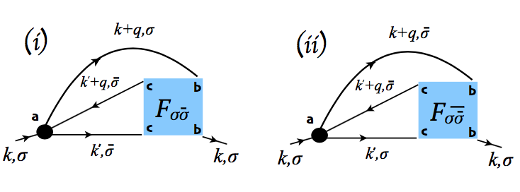
Figure 2: Diagrammatic representation of the non-local corrections to $\Sigma$ stemming from the fluctuations in longitudinal (i) and in the transverse (ii) channel within the ladder D$\Gamma$A for the AF phase.

Conversely, in the third one, only local terms ($\mathcal{F}^{loc}_{b,\sigma\bar{\sigma}}$) are present and there is no internal summation over the sub-lattice index. We show the diagrams corresponding to the longitudinal and transverse contributions in Fig. 2. Finally, it is worth noting, that it is possible to express the self-energy using the physical basis representation for ladders by simply inverting the relations in Tables  3,3.

V AF-D$\Gamma$A results with a mean-field input

To illustrate how the ladder-D$\Gamma$A equations derived in the previous sections work in practice, we present below a simplified, albeit fundamental application of our scheme to AF-ordered phase of the $2D$-Hubbard model at $T=0$.

Specifically, the approximated calculations of collective modes and the spectral properties presented in this section have been performed by evaluating all the D$\Gamma$A expressions for the AF phase (AF-D$\Gamma$A) starting from a static mean-field input (instead of the DMFT one). Diagrammatically, this corresponds to retain the lowest order contributions in $U$ for both the 1PI local self-energy and the 2PI local vertex appearing in the BSE and Schwinger-Dyson equations of the D$\Gamma$A for the AF-ordered system.

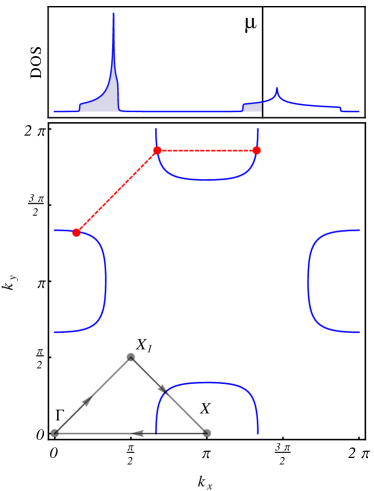
Figure 3: Lower panel: Fermi surface of the mean-field solution of the AF-ordered phase for the electron doped case (ii), with $n=1.2$ and $t^{\prime}/t=0.45$; the path indicated by the gray arrows is the specific one exploited in the following Figures; the red dashed lines mark particle-hole excitations connecting the same/different pockets on the FS (s. text). Upper panel: Corresponding density of states (DOS).

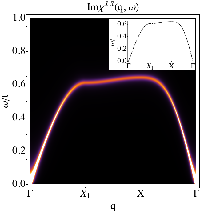
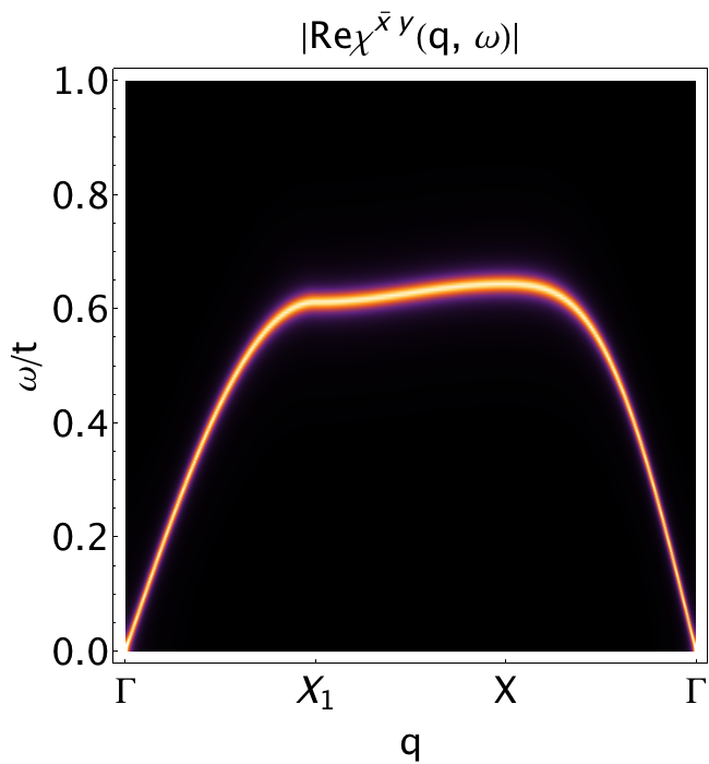
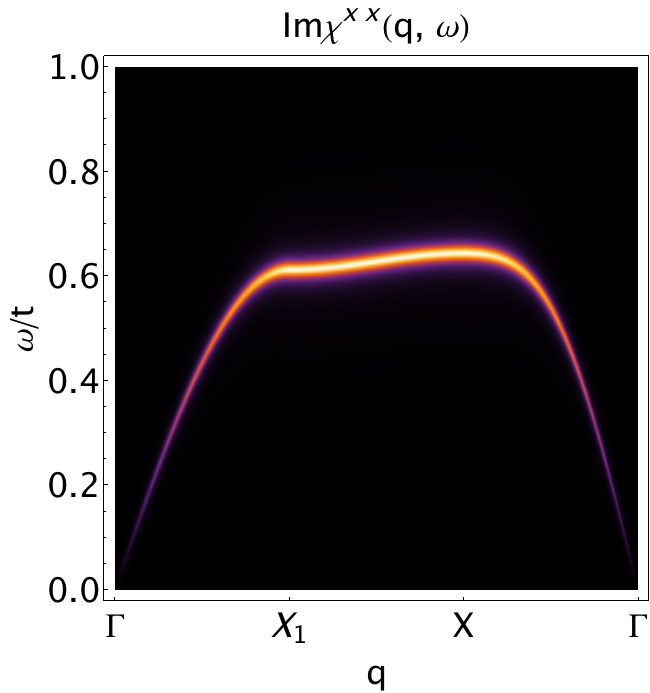
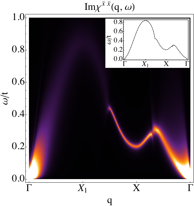
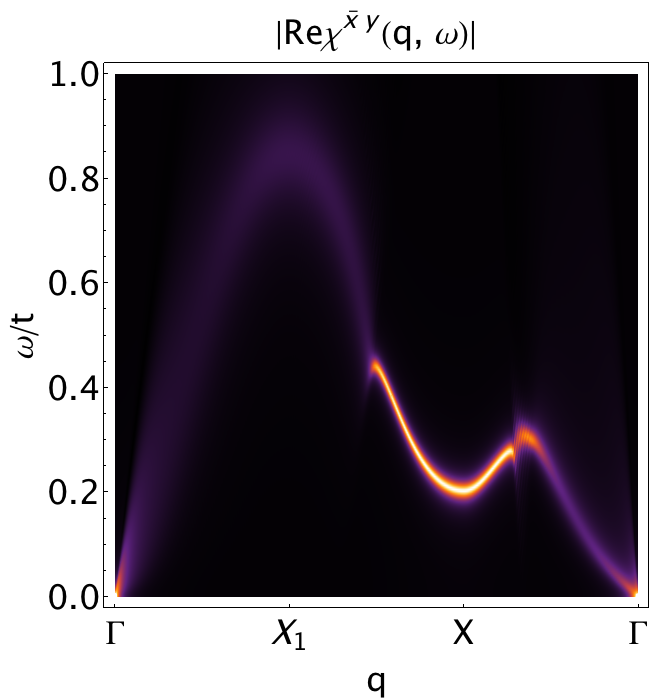
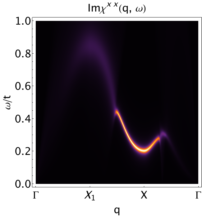
Figure 4: Intensity plot of the imaginary/real (absorption) part of the transverse susceptibilities $\chi_{\bar{x}\bar{x}}$, $\chi_{\bar{x},y}$,$\chi_{xx}$ (in arbitrary units) of the AF phase as a function of momentum (along the path shown in Fig. 3) and frequency computed at $T=0$ through the RPA-expression Eq. (92) for the particle-hole symmetric case (upper panels) and for the electron-doped case (lower panels). All expressions have been evaluated for a (retarded) frequency $z=\omega+i\delta$, with $\delta=0.01$. The brightest colors refers to the highest intensity values, while the black colors indicates a vanishing intensity. In the insets we show, as a guide to the eye, the dispersion relations of the corresponding magnons.

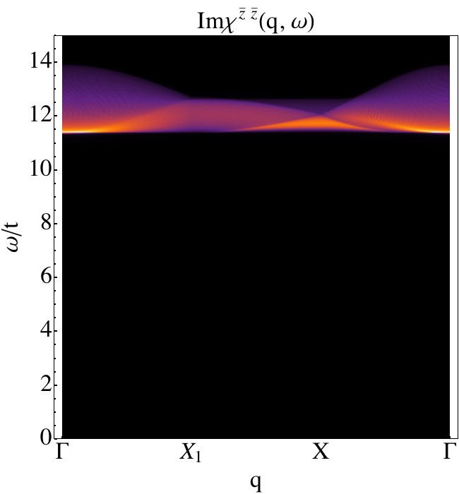
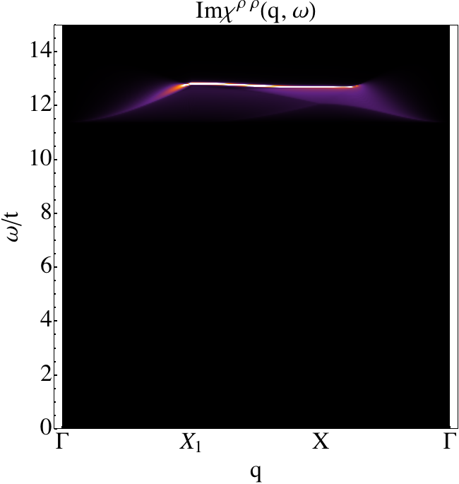
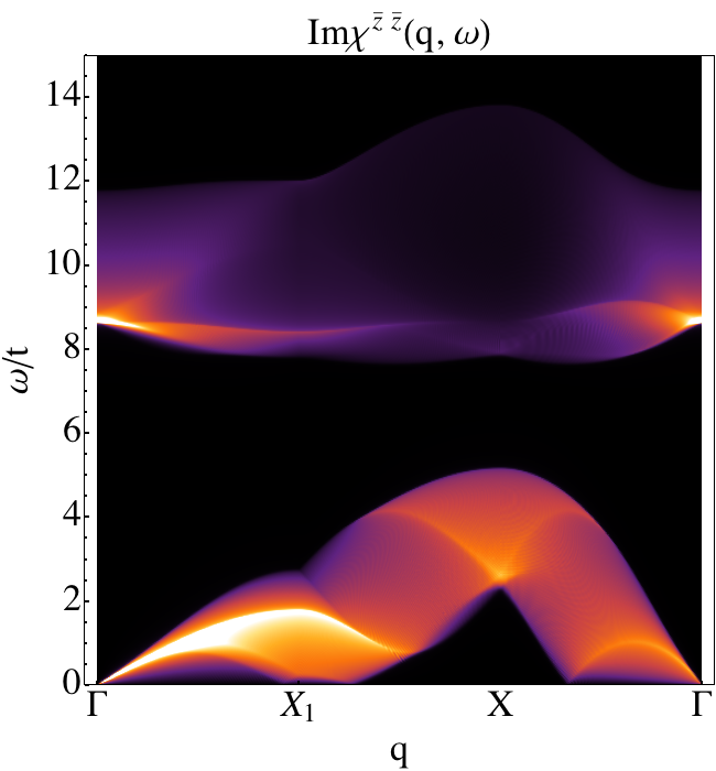
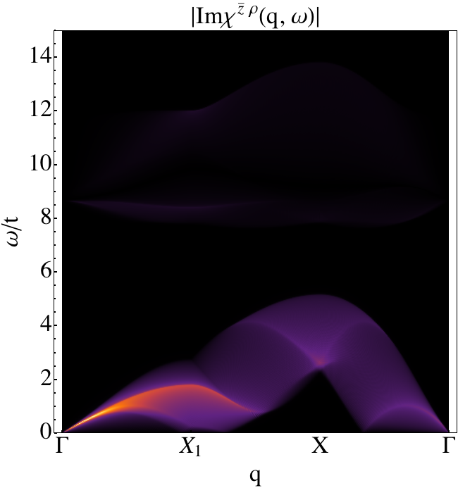
Figure 5: Same as in Fig. 4 but for the spin longitudinal channel. (Upper panels) $\chi_{\bar{z}\bar{z}}$, $\chi_{\rho\rho}$ are shown for the particle-hole symmetric case for the particle hole case. (Lower panels) The susceptibilities $\chi_{\bar{z}\bar{z}}$, $\chi_{\bar{z}\rho}$ are displayed for the electron-doped case. The corresponding expressions have been evaluated for a (retarded) frequency $z=\omega+i\delta$, with $\delta=0.01$.

Within this framework, the irreducible vertex function reduces to the bare interaction, as in RPA. Hence, under this assumption and using Eqs. (II.2,IV.2,IV.2) the physical susceptibilities read:

$$\bar{\bar{\chi}}_{{\overline{\sigma\bar{\sigma}}}}(q) = \bar{\bar{\chi}}_{{0\overline{\sigma\bar{\sigma}}}}(q)-\bar{\bar{\chi}}_{0\overline{\sigma\bar{\sigma}}}(q)\cdot\bar{\bar{\Gamma}}_{{\overline{\sigma\bar{\sigma}}}}\cdot\bar{\bar{\chi}}_{{\overline{\sigma\bar{\sigma}}}}(q),$$ (92)

$$\bar{\bar{\chi}}_{\parallel,\,\pm}(q) = \bar{\bar{\chi}}_{0\parallel,\,\pm}(q)-\bar{\bar{\chi}}_{0\parallel,\,\pm}(q)\cdot\bar{\bar{\Gamma}}_{\parallel}\cdot\bar{\bar{\chi}}_{\parallel,\,\pm}(q),$$ (93)

with $\bar{\bar{\chi}}_{0}(q)\equiv\frac{1}{(V\beta)^{2}}\sum_{k_{1}k_{2}}\bar{\bar{\chi}}^{k_{1}k_{2}q}_{0}$, $\bar{\bar{\Gamma}}_{\overline{\sigma\bar{\sigma}}}=-U\mathbbm{1}$ and $\bar{\bar{\Gamma}}_{\parallel}=U\tau^{(x)}$. Within this scheme, we now proceed to explicitly calculate the D$\Gamma$A self-energy of the broken-symmetry phase. Because of the chosen mean-field input for the irreducible vertex of the BSEs, the full vertex of the SDE will depend on the exchanged four momentum only, i.e. $F(k,k^{\prime},q)\sim F(q)$. Moreover, if we are away from (quantum) critical points, one could argue that the most important contributions to the D$\Gamma$A self-energy originates from the transverse spin sector, in which the gapless Goldstone modes arise. Therefore, Eq. (IV.3) can be simplified into:

$$\Sigma^{ab}_{\sigma}(k)-\delta_{ab}Un_{a,\bar{\sigma}} \sim \frac{U^{2}}{V\beta}\sum_{q}G^{ab}_{\bar{\sigma}}(k+q)\chi^{ab}_{\overline{\sigma\bar{\sigma}}}(q),$$

where $\chi^{ab}_{\overline{\sigma\overline{\sigma}}}(q)$ is defined in Eq. (92).

The aim of the calculations presented below is -anyway- more ambitious than presenting a mere proof-of-principle of our scheme. On the contrary, our results, obtained in a precisely controlled framework, will provide a reliable “compass” for future computational benchmarks and, above all, for the physical interpretation of more complex developments and applications.

In the following, we examine two specific realizations of the AF order in a two-dimensional Hubbard model at $T=0$, corresponding to rather distinct physical situations: (i) a half-filling (particle-hole) symmetric case (with $U/t=12$, $\mu=\frac{U}{2}$, $\Delta/t=5.69$) and (ii) a electron-doped case (with $U/t=12$, $\alpha=t^{\prime}/t=0.45$, $n=1.2$, that corresponds to $\mu/t=3.55$ and , $\Delta/t=4.32$). Consistent with the results by Igoshev et al.Igoshev et al. (2010), static mean-field (Hartree-Fock) calculations yield stable AF-order ground states for both parameter sets. The mean-field solutions of the two cases differ qualitatively: The former is insulating, while the latter is metallic, with the Fermi surface shown in Fig. 3.

Consistent with the derivations of Sec. IV, we will first analyze the numerical results for the main physical ingredient of the ladder D$\Gamma$A, namely the collective modes in the magnetic sector, and, thereafter, we will discuss the corresponding effects on the electronic self-energy.

V.1 Collective modes

Within our simplified D$\Gamma$A framework, the expression of the collective modes (and of the associated BSEs) coincide to the RPA ones in the AF long-range ordered phaseChubukov and Frenkel (1992); Rowe et al. (2012).

We start by considering the half-filling case (i). We show in Fig. 4 (upper panels for (i)) the results for absorption intensity of three independent transverse (Goldstone) modes: the odd $\chi_{\bar{x}\bar{x}}$, $\chi_{\bar{x}y}$ and the even $\chi_{xx}$, defined in Tab. 3 (see the Appendix for more details). The results can be easily interpreted by recalling that, while all Goldstone modes share the same denominator (and, hence, the same dispersion), they differ in the numerators. In particular, by performing a hydrodynamic expansion of the latter, one gets numerators which scale in frequency with different behaviors ($\omega^{0}$, $\omega$ and $\omega^{2}$ for $\bar{x}\bar{x}$, $\bar{x}y$ and $xx$, respectively). This makes, as one expects, the staggered $\bar{x}\bar{x}$ (non-staggered $xx$) Goldstone mode the most (least) dominant one at low-energies, with the $\bar{x}y$ displaying an intermediate behavior, as it can be readily seen in the intensity plots of Fig. 4.

Not surprisingly for the particle-hole symmetric case under consideration, the intensity plots of the corresponding longitudinal modes ($\chi_{\bar{z}\bar{z}}$ and $\chi_{\rho\rho}$, in the upper panels of Fig. 5) are rather featureless, due to a significant energy gap of $2\Delta$ controlled by the large value of the order parameter $m_{S}$.

We turn now to analyze the results obtained for the electron-doped case (ii).

By comparing the intensity plots of transverse (lower panels in Fig. 4) and longitudinal modes (lower panels in Fig. 5) to the corresponding half-filling results (upper panels), it is easy to visualize how the collective modes are affected by the low-energy fermionic quasi-particle excitations emerging in the doped case.

In particular, we note the appearance of a significant absorption in the low-energy regime for all longitudinal susceptibilities, readily interpreted in terms of the continuum of particle-hole excitations (lower panels in Fig. 5). With respect to this low-energy feature, the previously dominating high-energy branches appear now significantly damped. The interplay with these particle-hole excitations is also responsible for a visible smearing out of all Goldstone modes over broad regions of the BZ (s. lower panels of Fig. 4).

In the lower panels of Fig. 5, we observe that the absorption intensity increases in the vicinity of the $\Gamma$ point: This is due to particle-hole excitations that connect two points of the same Fermi pocket (e.g., horizontal red dashed line in Fig. 3). The intensity also increases close to $X_{1}$: This is due, instead, to particle-hole excitations connecting two points lying on different Fermi pockets (e.g., oblique red dashed line in Fig. 3).

A noticeable exception is represented by the large-momenta interval around $X$: Given the geometry of the underlying FS, for these values of ${\bf q}$ and $\omega$, it is not possible to generate particle-hole excitations. Furthermore, sizable change of slope of the Goldstone mode along the path $X\rightarrow\Gamma$ can be observed by comparing the results of the insulating (upper panels in Fig. 4) and the metallic AF (lower panels in Fig. 4) .

The numerical results shown in the lower panels of Fig. 4 can be rationalized by performing a hydrodynamic expansion of the susceptibility expressions. Precisely, we analyze their bubble-terms contributions which, within this simplified D$\Gamma$A context, completely control the momentum/frequency dependence of the corresponding susceptibilities. While referring to the Appendix for details, we briefly discuss here the main outcome. The bubble-terms in the AF phase consist of two contributions:

$$\chi_{0}(\mathbf{q},\omega)=\chi_{0,\mbox{\footnotesize inter}}(\mathbf{q},\omega)+\chi_{0,\mbox{\footnotesize intra}}(\mathbf{q},\omega)$$

i.e., the interband and the intraband terms. The former is always present for an AF-ordered system, while the latter becomes relevant for metallic solutions, e.g., in case (ii). In fact, while $\chi_{0,\mbox{\footnotesize inter}}(\mathbf{q},\omega)$ is responsible for the main structures of the Goldstone and the Higgs modes, shown in Figs. 4 and 5, $\chi_{0,\mbox{\footnotesize intra}}(\mathbf{q},\omega)$ acquires a singular part in the presence of a FS. Specifically, this happens when the hydrodynamic expansion of the quasi-particle dispersion along the Goldstone mode ($\omega=c|{\bf q}|$) intersects the FS. Quantitatively, this corresponds to the condition $c<4\,\alpha t\,q_{F}$, where $q_{F}=\sqrt{(\mu+4\alpha t-\Delta)/{2\alpha t}}$ is the absolute value of the Fermi momentum. The leading order contributions at low-energy is given by:

$$\chi_{0,\mbox{\footnotesize intra}}^{xx} = A\,q_{F}^{4}\,I^{xx}\left(\frac{\omega}{4\alpha t\,q_{F}\,|\mathbf{q}|},\cos 4\theta\right)$$ (95)

where $A=\frac{1}{[4\pi\,(\Delta/t)]^{2}\,\alpha t}$ , $\Delta=m_{S}U/2$, $m_{S}$ being the staggered magnetization. $I^{\alpha,\beta}(x_{1},x_{2})$ (see Appendix E) are complex functions of their arguments (whereas $\theta$ is the angle defining a direction in the BZ).

The non-vanishing imaginary part of these functions is responsible for the broadening of the Goldstone modes discussed above, while their explicit dependence on $\theta$ reflects in a corresponding angular modulation of the modes. In the AF metallic case, thus, the angular modulation appears already at the leading order in the hydrodynamic expansion, consistent with the numerical results shown in the lower panels of Fig. 4.

Finally, the continuum of particle-hole excitation is also responsible for a sizable coupling between the modes in the longitudinal section, as evidenced by the intensity-plot in the second of the lower panels of Fig. 5, referring to $\chi_{\bar{z}\rho}$. The intensity of such coupling, vanishing exactly for the particle-hole symmetric case [see Eq.(32)], tends to increase by increasing interaction. Hence, if not properly included in RPA calculations, it might yield significant corrections in the intermediate-to-strong coupling regime.

V.2 The self-energy in the AF-phase

The expression of the self-energy in Eq. (V) has been exploited for the two selected cases considered above. In the particle-hole/half-filled situation, the mean-field solution is fully gapped and this considerably quenches the D$\Gamma$A self-energy, because no fermionic/quasiparticle singularity is coupled to the massless Goldstone modes. Hence, in this case, the D$\Gamma$A corrections to the mean-field expressions reduce essentially to a quantitative renormalization of the staggered magnetization, as discussed in Refs. [Singh and Tešanović, 1990; Chubukov and Frenkel, 1992]. In particular, we found that, in the limit of a strong Coulomb interaction $U\gg t$, the quasi-particle residue is given by $Z_{qp}=\frac{1}{2}\left(1+\frac{1}{\sqrt{1+2\kappa}}\right)$, with $\kappa=\frac{1}{V}\sum_{\mathbf{q}}\frac{1-\sqrt{1-\gamma_{\mathbf{q}}^{2}}}{\sqrt{1-\gamma_{\mathbf{q}}^{2}}}\sim 0.39$, where $\gamma_{\mathbf{q}}=\frac{1}{2}[\cos q_{x}+\cos q_{y}]$ and the staggered magnetisation is renormalized by a factor $2\,Z_{qp}-1$. If we expand $Z_{qp}$ linearly in $\kappa$, the renormalization factor becomes $1-\kappa\sim 0.61$, consistent with Ref. [Chubukov and Frenkel, 1992] as well as the result obtained in spin-wave theory for the Heisenberg model.

Much more interesting are the D$\Gamma$A results out-of-half filling. Here, the presence of an underlying Fermi-surface in the mean-field solution allows for important D$\Gamma$A self-energy corrections, originated by the combined effect of bosonic (Goldstone) and fermionic (quasiparticles) excitations. Our numerical results are shown in Fig. 6, where we report explicitly the momentum dependence of the real and the imaginary part of the self-energy for the sub-lattice $A$ in the whole BZ (upper panels), and at the same time, its frequency dependence at four selected k-points (lower panels).

In order to clarify the overall behavior of the self-energy in the AF phase, it is convenient to consider separately the high-frequency and the low-frequency regime.

As we discuss below, the former is controlled by precise analytical relations, which extends the well known ones for the SU(2)-symmetric case. By inverting the relations in Table 3, we can express the equation of motion in terms of the susceptibilities in the physical basis as following:

$$\chi^{ab}_{\overline{\sigma\overline{\sigma}}}(q) = \frac{1}{2}\left[\chi^{xx}(q)+(-1)^{a+b}\chi^{\bar{x}\bar{x}}(q)\right]$$ (96)

$$- \delta_{ab}(-1)^{a}\,i\sigma\,\chi^{x\bar{y}}(q).$$

Then, from Eqs.(V,96), we can extrapolate the asymptotic behavior of $\Sigma$ in the limit of large frequencies. Specifically, for $\nu\to\infty$, we have:

$$\nu\,\mbox{Im}\Sigma_{\sigma}^{ab}(k)=\mbox{const.}=-U^{2}\delta_{ab}\frac{1}{V\beta}\sum_{\omega}\sum_{\mathbf{q}\in BZ}\left[\chi^{xx}(q)+(-1)^{a}\,\sigma\,m_{S}\,\mbox{Re}G^{aa}_{\bar{\sigma}}(q+k_{0})\right],$$ (97)

where we defined $k_{0}=(\boldsymbol{0},\nu_{0})$ for compactness of notation. We observe that, since the integrand function in Eq.(V) is even under a shift of $\Pi=(\pi,\pi)$ of the exchanged momentum, the summation in Eq.(97) can be extended to the entire BZ. It is interesting to notice that, in the broken-symmetry phase, the high-frequency asymptotic behavior of $\Sigma$ depends both on the electronic density and on the order parameter. This marks a qualitative difference from the normal phase, where the high-frequency asymptotics of $\Sigma$ is controlled by electronic density only. Specifically, the constant prefactor $m_{S}$ originates from the mixed correlator $\chi^{x\bar{y}}$, which, as pointed out in Sec.II.2, is related to the order parameter through the commutation relation between the spin operators. The non-trivial match between the analytic/expected expressions for the high-frequency behavior of the self-energy and our numerical calculations is explicitly shown for the case of the four selected k-point in the leftmost bottom panel of Fig. 6. Such numerical agreement has been verified for all momenta, providing an useful double-check for the algorithmic implementation of the AF-D$\Gamma$A expression.

Let us now focus on the low-energy properties of $\Sigma$. In the presence of an underlying Fermi surface, one expects that the most important information will be encoded in the corresponding Fermi energy and momenta. The data shown in Fig. 6 appear consistent with such expectation: One can readily identify the region of the Brillouin-zone, where the D$\Gamma$A corrections induce the strongest momentum dependence in the low-frequency self-energy. In particular, the data reported in the upper panels of Fig. 6 clearly show how the largest variation of both real and imaginary parts of $\Sigma_{AA}$ over the whole Brillouin zone occurs in the proximity of the underlying Fermi-surface of the mean-field solution (cf. Fig. 3). Specifically, by crossing the FS, both Im$\Sigma_{AA}$ (left upper panel of Fig. 6) and Re$\Sigma_{AA}$ (right upper panel of Fig. 6) get strongly enhanced in absolute value, whereas Re$\Sigma_{AA}$ also displays an evident change-of-sign. More quantitatively, we observe over the whole FS a simultaneous divergence of both imaginary and real part of $\Sigma_{AA}$ in the zero-frequency limit, though with a different degree of severity. It should be also noted that the additional, and rather weak, sign-structures (oblique blue linear-shaped regions in the intensity plot of Re$\Sigma_{AA}$) essentially reflect the halving of the BZ due to the AF-order.

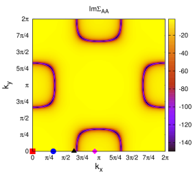
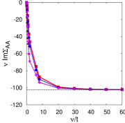
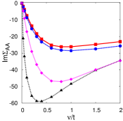
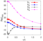
Figure 6: (Upper Panels) Color intensity plots of the imaginary part (on the left) and real part (on the right) of the majority spin self-energy of the sublattice $A$ in the AF-phase as a function of the momenta calculated at the imaginary frequency $\nu/t=0.025$, for $U/t=12$, $n=1.2$ and $\alpha=0.45$. (Lower Panels) The the high frequency behavior of the self energy is reported in the leftmost panel, the thin line marking the asymptotic value defined in Eq. (97). The imaginary part (center) and real part (right) of the self-energy are shown as a function of the imaginary frequency $\nu$ for four ${\mathbf{k}}$-points lying on the $\Gamma$-X direction in the BZ and marked by different colors/symbols in the upper panels.

As we detail in the following, the self-energy behavior shown in Fig. 6 is the direct consequence of the combined action of the massless Goldstone modes and quasiparticle excitations at the Fermi level, which we mentioned before. The physical mechanism is indeed similar to the one triggering the enhanced scattering rate observed in several D$\Gamma$A studies of the SU(2)-symmetric phases in the proximity of phase-transitions (in $d=3$)Rohringer et al. (2011); Rohringer and Toschi (2016); Rohringer et al. (2018); Del Re et al. (2019) and/or for very large value of the magnetic correlation length (in $d=2$) Schäfer et al. (2015, 2016a). In the broken-symmetry phase, however, the analogy is not complete. In fact, due to the finite value of the order parameter and of the corresponding doubling of the unit cell, the large self-energy corrections, evidenced by the color changes in Fig. 6 do not correspond to a significant loss of coherence in the low-energy fermionic excitations.

In order to elucidate the physics encoded in the D$\Gamma$A self-energy of the AF-phase, we explicitly analyze the zero-energy poles of the corresponding Green’s function as well as the the associated quasi-particle renormalization. For capturing the low-frequency behavior of the self-energy we can keep just $\chi^{\bar{x}\bar{x}}$ in Eq. (96), that accounts for the leading divergent orders when $\omega\sim 0$. Furthermore, we can approximate $G_{\bar{\sigma}}^{ab}(k+q)\sim G_{\bar{\sigma}}^{ab}(\mathbf{k},\omega+\nu)$, as we want to keep only the $\mathbf{q}\sim 0$ contributions in the integral in Eq.(V). Under these assumptions the equation of motion for $\bar{\bar{\Sigma}}_{\sigma}(k)-\delta_{ab}Un_{a,\bar{\sigma}}$ reads:

$$\sim \frac{U^{2}}{(2\pi)^{d+1}}\int_{-\infty}^{+\infty}d\omega\int_{BZ}d\mathbf{q}\,\chi^{\bar{x}\bar{x}}(q)\,\tau^{(y)}\cdot\bar{\bar{G}}_{\sigma}(\mathbf{k},\omega+\nu)\cdot\tau^{(y)}.$$

We can now express the self-energy in the basis of the quasi-particles, i.e.

$$\bar{\bar{\Sigma}}_{\sigma}(k)-\delta_{ab}Un_{a,\bar{\sigma}}=e^{-i\tau^{(y)}\theta_{\mathbf{k}\sigma}}\tau^{(y)}\left(\begin{array}[]{cc}\sigma^{+}_{\mathbf{k}}(\nu)&0\\ 0&\sigma^{-}_{\mathbf{k}}(\nu)\end{array}\right)\tau^{(y)}\,e^{i\tau^{(y)}\theta_{\mathbf{k}\sigma}}=e^{-i\tau^{(y)}\theta_{\mathbf{k}\sigma}}\left(\begin{array}[]{cc}\sigma^{-}_{\mathbf{k}}(\nu)&0\\ 0&\sigma^{+}_{\mathbf{k}}(\nu)\end{array}\right)e^{i\tau^{(y)}\theta_{\mathbf{k}\sigma}},$$ (98)

where:

$$\sigma_{\mathbf{k}}^{\pm}(\nu)=\frac{U^{2}}{(2\pi)^{d+1}}\int_{-\infty}^{+\infty}d\omega\int_{BZ}d\mathbf{q}\,\,\frac{\chi^{\bar{x}\bar{x}}(q)}{i\nu+i\omega-\omega^{\pm}_{\mathbf{k}}},$$

and after carrying out the integrals we have:

$$\sigma^{\pm}_{\mathbf{k}}(\nu\to 0)\propto-\mbox{sign}\left(\omega^{\pm}_{\mathbf{k}}\right)\mbox{ln}\left(\frac{1}{\left|\omega_{\mathbf{k}}^{\pm}\right|}\right)-i\,\frac{\nu}{\left|\omega^{\pm}_{\mathbf{k}}\right|}.$$ (100)

Hence, for $d=2$, logarithmic and power-low divergences appear in the real and imaginary part and the self-energy, respectively, when $\mathbf{k}\in$ FS. It is important to note, however, that the doubling of the unit cell associated to the AF phase does prevent the quasi-particle excitations to be washed out by such divergences.

To explain this, let us first notice that the self-energy in Eq. (98) is diagonal in the HF quasi-particles basis. Therefore, in this reference frame, the Dyson equation reads:

$$\bar{\bar{G}}^{-1}_{\mathbf{k}}(\nu)\sim\left(\begin{array}[]{cc}i\nu-\omega^{+}_{\mathbf{k}}-\sigma^{-}_{\mathbf{k}}(\nu)&0\\ 0&i\nu-\omega^{-}_{\mathbf{k}}-\sigma^{+}_{\mathbf{k}}(\nu)\end{array}\right).$$ (101)

The conduction band is dressed with the self-energy $\sigma^{-}_{\mathbf{k}}(\nu)$ that depends on the valence electrons energy $\omega^{-}_{\mathbf{k}}$. The presence of a gap prevents $\sigma_{\mathbf{k}}^{-}(\nu)$ to diverge and the FL excitations are stable.

Conversely, the valence electrons are dressed with the self-energy $\sigma_{\mathbf{k}}^{+}(\nu)$, which diverges when $\nu\to 0$ at the FS.

We support our analytical findings by showing in Fig. 7 the numerical values of the Green’s function zero-energy poles $\Lambda^{\pm}_{\mathbf{k}}$, which defines two bands. The first one, $\Lambda^{+}_{\mathbf{k}}$ is a smooth function of the crystal momentum and represents a conduction band, which emerges from a sizable reshaping of the corresponding one in the HF solution. In fact, it is only the second (valence) band ($\Lambda^{-}_{\mathbf{k}}$) to be affected by logarithmic singularities, which precisely appear when HF-conduction band crosses the Fermi level, as it is clearly shown in Fig. 7.

On the basis of these considerations and of our numerical results, we can conclude that the conduction band is stable under non-local quantum fluctuations: In spite of the large (or even diverging) values of Im $\Sigma$, the metallic coherence of the corresponding low-energy quasi-particle excitations is preserved.

At the same time, this analysis does not provide specific information about what happens at higher energy. In fact, to understand properly how the valence band is dressed by the conduction electrons we should numerically evaluate the Green’s function on the real frequency axis. While this is beyond the aim of the present work, we expect -in general- that such corrections will affect the way how the high-energy spin excitations, such as the sharp spin-polaronsStrack and Vollhardt (1992); Sangiovanni et al. (2006) clearly visible at DMFT levelStrack and Vollhardt (1992); Sangiovanni et al. (2006); Taranto et al. (2012), reshape the spectral functions and the charge/optical response of the system.

In this perspective, future applications of our ladder D$\Gamma$A approach exploiting a full DMFT input (possibly directly computed on the real frequency axisKugler et al. (2021); Lee et al. (2021)) could provide a very powerful set-up to investigate the spin-polaron physics in realistic three- or two-dimensional cases. In particular, one would aim at estimating the broadening of the spin-polaron peaks induced by non-local correlations beyond DMFT and at identifying fingerprints of these excitations in the physics of bulk and layered antiferromagnets.

On a broader perspective, the results of this section shed light on the general physical behavior to be expected in metallic systems in the presence of magnetic order and/or strong magnetic fluctuations. The onset of a long-range AF order shifts the major effects of the magnetic correlations on the electronic spectra from low- to higher frequencies. Even when such effects are -per se- strong, as it happens in correlated metals due to the cooperative action of Goldstone modes and quasi-particles, the coherent nature of the underlying Fermi-liquid excitations remains preserved, if the order parameter is large enough. Hence, the largest quasi-particle scattering rates is expected to occur in critical or quantum critical regimes of (here: magnetic) phase-transitions. The possible occurrence of a minimal metallic coherence at the phase-transition is compatible with the results of previous numerical studiesRohringer and Toschi (2016) performed in the proximity of a AF-transition of the Hubbard model in $d\!=\!3$. It is also consistent with several spectroscopic/transport observations made in the (almost bidimensional) cuprates when cooling the compounds below their superconducting transition temperature in the underdoped/optimally doped regime.

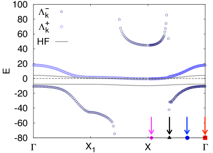
Figure 7: Plot of the lower and upper eigenvalue $\Lambda^{\pm}_{\mathbf{k}}$ represented respectively by pentagons and circles as a function of the momentum. We plotted the bands obtained in Hartree-Fock (gray solid lines) as a reference. The four arrows pointing onto the $x$-axis mark the corresponding momenta selected in Fig. 6.

VI Conclusions and Outlook

In this work, we have illustrated how to extend the ladder D$\Gamma$A approach, hitherto restricted to the SU(2) symmetric case, to the treatment of electronic correlations in magnetic systems, with ferromagnetic or antiferromagnetic long-range order.

In particular, starting by general considerations on the two-particle vertex functions in the limit of infinite dimensions/coordination of the lattice, we have first generalized the condition of pure locality for the irreducible vertices of DMFT to solutions with magnetic order. Secondly, we have exploited the corresponding Bethe-Salpeter/ladder equations, which describe the longitudinal/transverse collective modes at the level of DMFT, to derive, through the Schwinger-Dyson relations, the ladder D$\Gamma$A expression for the electronic self-energy of the magnetically ordered phases.

To demonstrate the applicability of our extended D$\Gamma$A approach, we have exploited it to study a couple of simplified, but representative model cases with AF-order, where we approximated the DMFT input of the D$\Gamma$A equations to its static mean-field counterpart. In this framework, the collective modes inducing the non-local D$\Gamma$A correlation reduces to the corresponding RPA ones. The reported results represents a solid benchmark for future, more demanding calculations. At the same time, the thorough analysis of the self-energy results in the non-particle hole symmetric-case allows us to outline important physical effects to be expected in the correlated magnetic systems, in particular concerning the coherence of the underlying electronic excitations.

Analogously as in the first ladder D$\Gamma$A derivation for the SU(2)-symmetric caseToschi et al. (2007), we have considered here the most fundamental implementation of the approach. This consists in a single-shot correction of the DMFT results originated by the scattering with the corresponding magnetic modes. The question arises whether it is possible and/or convenient to implement a self-consistent version of the ladder D$\Gamma$A equations in the broken SU(2)-symmetric case. While this issue certainly calls for a dedicated study, analogous to Refs. [Katanin et al., 2009; Rohringer and Toschi, 2016; Rohringer et al., 2018; Kaufmann et al., 2020], we observe here that additional constraints must be taken into account in the magnetically ordered phase. For example, one could try extend the so-called $\lambda$-correction, introduced within a’ la Moriya schemesKatanin et al. (2009); Rohringer and Toschi (2016), to the FM/AF case. The underlying idea, which can be regardedDel Re et al. (2019) -to some extent- as a dynamical version of the Two Particle Self-Consistent (TPSC) approachVilk and Tremblay (1997), consists in constraining some important parameter of the theory (e.g., the mass of the spin propagator) to fulfill physically relevant relations, such, e.g., the asymptotic high-frequency behavior of the D$\Gamma$A self-energy. Evidently, this task gets significantly harder in the broken SU(2)-symmetry phase, because of the increased number of independent degrees of freedom (see Tabs. 1- 3-3), and the precise interrelations between them which need to be preserved. At the same time, the identification of the physical relations to be enforced is less obvious than in the symmetric case, as well exemplified by the expression for high-frequency asymptotics of the self-energy in the AF-phase given in Eq. (97).

Another possibility would be to implement a true self-consistent loop, by inserting the momentum-dependent expression of the D$\Gamma$A self-energy back in the Bethe-Salpeter equations, while keeping fixed the (local) irreducible vertices, in a similar spirit of the so-called “internal” self-consistency of the DF approachRubtsov et al. (2008); Rohringer et al. (2018) and of the most recent algorithmic developmentKaufmann et al. (2020) of the ladder D$\Gamma$A in the SU(2)-symmetric case. This route would avoid all the preliminary, physically-motivated ad hoc implementations of a la Moriya correction schemes, requiring, however, a higher numerical effort. In any case, it needs to be verified, whether such self-consistent ladder implementation can guarantee a coherent description of the instability driven by an external parameter ($T$, $n$, $h$, …) from both sides (ordered and disordered) of the magnetic transition. From the technical point of view, one should also ensure that the massless nature of the Goldstone modes remains preserved at every iteration.

While these considerations might serve as guidance for future methodological advancements in the description of correlated magnetic systems, our preliminary study suggests that interesting results can be obtained by means of the one-shot ladder D$\Gamma$A scheme presented here, especially for investigating the non trivial behavior of the spectral properties of correlated magnets in the proximity of their classical or quantum phase-transitions.

Finally, the explicit analytical expressions for the collective modes given in Tabs. 1-3-3 and the self-energy of the magnetically ordered phases could be quite inspiring for future extensions of the recently introduced fluctuation diagnostics post-processing methodsGunnarsson et al. (2015); Rohringer (2020); Schäfer and Toschi (2021) and fluctuation analysis of the two-particle irreducible vertex functionDel Re and Rohringer (2021) to the broken SU(2)-symmetry phases.

Appendix A Change of coordinates for four-point correlation functions

In this section we formally derive Eqs.(II.1,5,II.1,7). Let us first consider the case where $\hat{H}$ is left invariant under the unitary transformation $\psi_{\mathbf{R}}\to U^{\,}_{\mathbf{R}}\,\psi_{\mathbf{R}}$. Therefore, by expressing the Fermi fields in the new basis we can rewrite Eq.(1) as following:

$$[U^{\dagger}_{\mathbf{R}_{1}}]_{\alpha^{\prime}\alpha}[U^{\,}_{\mathbf{R}_{2}}]_{\beta\beta^{\prime}}[U^{\dagger}_{\mathbf{R}_{3}}]_{\gamma^{\prime}\gamma}[U^{\,}_{\mathbf{R}_{4}}]_{\delta\delta^{\prime}}\chi^{\alpha^{\prime}\beta^{\prime}}_{\gamma^{\prime}\delta^{\prime}}(x_{1},x_{2},x_{3},x_{4}),$$

where a summation over repeated indices is intended. Substituing Eq.(A) into Eq.(2) we obtain:

$$V^{a}_{\alpha\beta}(\mathbf{R}_{1},\mathbf{R}_{2})V^{b}_{\gamma\delta}(\mathbf{R}_{3},\mathbf{R}_{4})\chi^{\alpha\beta}_{\gamma\delta}(x_{1},x_{2},x_{3},x_{4}),$$ (103)

where $V^{a}(\mathbf{R},\mathbf{R}^{\prime})=U^{\dagger}_{\mathbf{R}}\,T^{(a)}\,U^{\,}_{\mathbf{R}^{\prime}}$. Choosing $T^{(a)}$ as a complete set of hermitian generators satisfying the orthonormality condition Tr$\left[T^{(a)}T^{(b)}\right]=\delta_{ab}$, we can express the $V^{a}$ matrix as a linear combination of the generators in the following way

$$V^{a}(\mathbf{R},\mathbf{R}^{\prime})=\sum_{b}\overbrace{\mbox{Tr}\left[T^{(b)}V^{a}(\mathbf{R},\mathbf{R}^{\prime})\right]}^{F_{\mathbf{R}\mathbf{R}^{\prime}}^{ab}}T^{(b)},$$ (104)

where the coefficents of the expansions are the same as those defined in Eq.(5). Substituting the last equation into Eq.103 we finally obtain Eq.(II.1).

Let us now consider a particle-hole transformation, i.e. $\psi^{\,}_{\mathbf{R}}\to U_{\mathbf{R}}^{\,}\psi^{{\dagger}}_{\mathbf{R}}$. Expressing the fermi operators in the new basis, we can rewrite Eq.(1) in the following way:

$$[U^{\dagger}_{\mathbf{R}_{1}}]_{\alpha^{\prime}\alpha}[U^{\,}_{\mathbf{R}_{2}}]_{\beta\beta^{\prime}}[U^{\dagger}_{\mathbf{R}_{3}}]_{\gamma^{\prime}\gamma}[U^{\,}_{\mathbf{R}_{4}}]_{\delta\delta^{\prime}}\chi^{\beta^{\prime}\alpha^{\prime}}_{\delta^{\prime}\gamma^{\prime}}(x_{2},x_{1},x_{4},x_{3})=$$

$$[U^{\dagger}_{\mathbf{R}_{1}}]_{\beta^{\prime}\alpha}[U^{\,}_{\mathbf{R}_{2}}]_{\beta\alpha^{\prime}}[U^{\dagger}_{\mathbf{R}_{3}}]_{\delta^{\prime}\gamma}[U^{\,}_{\mathbf{R}_{4}}]_{\delta\gamma^{\prime}}\chi^{\alpha^{\prime}\beta^{\prime}}_{\gamma^{\prime}\delta^{\prime}}(x_{2},x_{1},x_{4},x_{3}).$$

Substituting Eq.(A) in Eq.(2) yields:

$$\widetilde{V}^{a}_{\alpha\beta}(\mathbf{R}_{1},\mathbf{R}_{2})\widetilde{V}^{b}_{\alpha\beta}(\mathbf{R}_{3},\mathbf{R}_{4})\chi^{\alpha\beta}_{\gamma\delta}(x_{2},x_{1},x_{4},x_{3}),$$ (106)

where

$$\widetilde{V}^{a}_{\alpha\beta}=\sum_{\alpha^{\prime}\beta^{\prime}}[U^{\dagger}_{\mathbf{R}}]_{\beta\alpha^{\prime}}T^{(a)}_{\alpha^{\prime}\beta^{\prime}}[U^{\,}_{\mathbf{R}^{\prime}}]_{\beta^{\prime}\alpha}=\left[U^{\dagger}_{\mathbf{R}}\,T^{(a)}\,U_{\mathbf{R}^{\prime}}^{\,}\right]^{T}_{\alpha\beta}.$$

We can express this matrix using the same expansion as in Eq.(104), i.e.

$$\widetilde{{V}}^{a}(\mathbf{R},\mathbf{R}^{\prime})=\sum_{b}\mbox{Tr}\overbrace{\left[T^{(b)}\widetilde{V}^{a}(\mathbf{R},\mathbf{R}^{\prime})\right]}^{\widetilde{F}^{ab}_{\mathbf{R}\mathbf{R}^{\prime}}}T^{(b)},$$ (107)

whose coefficents are the same as those appearing in Eq.(7). After we substitute the last equation in Eq.(A), we obtain Eq.(II.1).

Appendix B Generic properties of mixed and non-mixed correlators

For completeness, here we show some generic properties of correlation functions evaluated along the imaginary axis. Let $\hat{A}$ and $\hat{B}$ be generic two-particle operators, whose time-evolution in the Heisenberg representation is driven by a time-independent Hamiltonian, and let us define the correlation function between them:

$$C_{AB}(\tau)=T_{\tau}\left<\hat{A}(\tau)\hat{B}(0)\right>,$$ (108)

and its Fourier transform as: $C_{AB}(\omega)=\int_{0}^{\beta}d\tau\,C_{AB}(\tau)\,e^{i\omega\tau}$, with $\omega=2n\,\pi\,T$ being a bosonic Matsubara frequency.

	$\hat{A}$	$\hat{B}$
(i)	$\hat{A}^{\dagger}$	$\hat{B}^{\dagger}$	$\begin{array}[]{ccc}C_{AB}^{*}(\tau)&=&C_{AB}(-\tau)\\ C_{AB}^{*}(\omega)&=&C_{AB}(\omega)\end{array}$
(ii)	$\hat{B}^{\dagger}$	$\hat{A}^{\dagger}$	$\begin{array}[]{ccc}C^{*}_{AB}(\tau)&=&C_{AB}(\tau)\\ C^{*}_{AB}(\omega)&=&C_{AB}(-\omega)\end{array}$
(iii)	$\hat{A}^{\dagger}$	$\hat{A}$	$\begin{array}[]{ccc}C_{AB}(\tau)&=&C_{AB}(-\tau)\in\mathbbm{R}\\ C_{AB}(\omega)&=&C_{AB}(-\omega)\in\mathbbm{R}\end{array}$

Table 5: Symmetry properties of correlation functions in imaginary time/frequency domain for the three different cases discussed in the main text. These relations can be derived starting from the definition in Eq. (108) and using the cyclic property of the trace and the fact that $C_{AB}(\tau)$ is a periodic function of period $\beta$.

In Table 5, we list the properties of the correlation function in three different cases:

1. $\hat{A}$ and $\hat{B}$ are two different Hermitian operators (mixed-correlator),
   

2. $\hat{A}$ and $\hat{B}$ are one the hermitian conjugate of the other (pair-like correlator),

3. $\hat{A}$ and $\hat{B}$ are identical and hermitian (auto-correlator).

In the paramagnetic case, mixed-correlators of different observables vanish and auto-correlators are bounded to be even functions of the Matsubara frequency. This implies that in the limit of $\omega\to\infty$ they must decay at least as $1/\omega^{2}$. In the broken symmetry phase, instead, nonzero mixed correlators, which are not bound any longer to be even functions of the frequency, might appear. In that case, they may decay as $1/\omega$ in the limit of large frequencies. Indeed, this is the case of the mixed correlator $\chi^{xy}$ in the FM or $\chi^{x\bar{y}}$ in AF as discussed in the main text, which has important consequences on the high frequency behavior (asymptotics) of the self-energy as we show in Sec. V.2.

Appendix C Analysis of the two-particle reducible diagrams

In this appendix, we illustrate through an inspection of the relevant diagrammatics, how the simplified structure of the two-particle reducible contributions in Eqs. (45,48) of the main text arises.

We consider explicitly the case of the $ph$ channel in the AF phase, starting from the diagrams for $\Phi_{\rm ph}$, but the derivation can be repeated straightforwardly for the other channels (as well as for the PM/FM cases).

Once again, we follow the strategy of focusing on the first corrections to purely local diagrams. Since non-locality is introduced by the reducible bubble terms, the representative three diagrams to be considered are those depicted in Fig. 8. Here all squared boxes correspond to purely local vertex contributions [e.g., ${\mathcal{V}}_{a}(\nu,\nu^{\prime},\omega)\delta_{ab}\delta_{bc}\delta_{cd}$]. These three examples (${\mathcal{P}}_{1}$, ${\mathcal{P}}_{2}$, ${\mathcal{P}}_{3}$) also correspond to the three classes in which reducible diagrams can be subdivided, in terms of their dependence of the basis-lattice index ($2$,$3$,$4$) as well as of high-frequency asymptotic propertiesRohringer et al. (2012); Tagliavini et al. (2018); Wentzell et al. (2020).

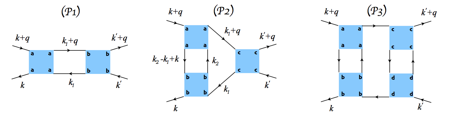
Figure 8: Representative contributions to $\Phi_{ph}$, the two-particle reducible vertex in the particle-hole channel in momentum space, see text. The labels $a,b,c,d$ run over the the lattice sites $A$,$B$.

As for ${\mathcal{P}}_{1}^{ab}(k,k^{\prime},q)$, one finds:

$${\mathcal{P}}_{1}^{ab} = \frac{1}{\beta V}\sum_{k_{1}}{\mathcal{V}}_{a}(\nu,\nu_{1},\omega){\mathcal{V}}_{b}(\nu_{1},\nu^{\prime},\omega)\,G_{ab}(k_{1})G_{ba}(k_{1}+q)$$

$$= \frac{1}{\beta}\sum_{\nu_{1}}{\mathcal{V}}_{a}(\nu,\nu_{1},\omega){\mathcal{V}}_{b}(\nu_{1},\nu^{\prime},\omega)\,{\mathcal{B}}^{ab}\left(\nu_{1},\omega,X({\bf q})\right)$$

(109)

where ${\mathcal{B}}^{ab}(\nu_{1},\omega,X({\bf q}))=\frac{1}{V}\sum_{\bf k_{1}}G_{ab}(k_{1})G_{ba}(k_{1}+q)$, where $G_{ab}$ is the Green’s funcion calculated in DMFT, that reads:

$$\bar{\bar{G}}_{\sigma}(k)=\frac{1}{\zeta_{A\sigma}(\nu)\zeta_{B\sigma}(\nu)-\epsilon_{\mathbf{k}}^{2}}\,\left(\begin{array}[]{cc}\zeta_{B\sigma}(\nu)&\epsilon_{\mathbf{k}}\\ \epsilon_{\mathbf{k}}&\zeta_{A\sigma}(\nu)\end{array}\right),$$ (110)

with $\zeta_{a\sigma(\nu)}=i\nu+\mu-\Sigma_{\sigma a}(\nu)$.

For the calculation of $\mathcal{B}_{ab}$ we could extend the summation over the whole BZ because the integrand function is symmetric under translation of $\boldsymbol{\Pi}$ .

Now we can express the bubble as a double integral with the integrand weighted by the two-particle density of states of the hyper-cubic lattice, i.e.

$$\mathcal{B}^{ab}(\nu,\omega,X)=\iint d\epsilon_{1}d\epsilon_{2}\,D^{X}_{\epsilon_{1},\epsilon_{2}}G_{ab}(\nu,\epsilon_{1})G_{ba}(\nu+\omega,\epsilon_{2}),$$ (111)

where the explicit expression of $D^{X}_{\epsilon_{1},\epsilon_{2}}$, which can be found in Ref. [Georges et al., 1996], has the following property $D^{X=0}_{\epsilon_{1},\epsilon_{2}}=g(\epsilon_{1})g(\epsilon_{2})$, with $g(\epsilon)$ being the DOS. The latter property implies that $\mathcal{B}^{ab}(\nu,\omega,0)=0$ when $a\not=b$ , because the off-diagonal terms of the Green’s function are odd in $\epsilon$ as opposed to the DOS that it is an even function. Instead, when $a=b$, $\mathcal{B}^{ab}(\nu,\omega,0)=\mathcal{B}_{loc}^{a}(\nu,\omega)=G^{AIM}_{a}(\nu)G_{a}^{AIM}(\nu+\omega)$. We can summarize these properties more concisely as follows:

$$\mathcal{B}^{ab}(\nu,\omega,X)=\delta_{ab}\,\mathcal{B}_{1}(\nu,\omega,X)+\delta_{a\bar{b}}\,\mathcal{B}_{2}(\nu,\omega,X),$$ (112)

where $\mathcal{B}_{1}(\nu,\omega,0)\!=\!G^{AIM}_{a}(\nu)G_{a}^{AIM}(\nu+\omega)$ and $\mathcal{B}_{2}(\nu,\omega,0)=0$.

Similarly, for ${\mathcal{P}}_{2\,c}^{\phantom{2}\,ab}(k,k^{\prime},q)$, we must perform the internal momentum summation over ${\bf k_{1}}$ and ${\bf k_{2}}$ in the corresponding bubble terms:

$$\frac{1}{V^{2}}\sum_{{\bf k}_{1},{\bf k}_{2}}G_{ab}(k_{2}-k_{1}+k)G_{ba}(k_{2})G_{ac}(k_{1}+q)G_{cb}(k_{1})$$

$$= \frac{1}{V}\sum_{\bf k_{1}}{\mathcal{B}}^{ab}(\nu_{2},\nu-\nu_{1},X({\bf k}-{\bf k}_{1}))\;G_{ac}(k_{1}+q)G_{cb}(k_{1})$$

$$= {\mathcal{B}}_{1}^{a}(\nu_{2},\nu-\nu_{1},X=0)\,\delta_{ab}\,\frac{1}{V}\sum_{\bf k_{1}}G_{ac}(k_{1}+q)G_{ca}(k_{1})$$

$$= {\mathcal{B}}^{a}_{1}(\nu_{2},\nu-\nu_{1},X=0)\,\delta_{ab}\,{\mathcal{B}}^{ac}(\nu_{1},\omega,X({\bf q}))\,,$$

where we used the fact that $\mathbf{k}-\mathbf{k}_{1}$ is a generic point in the BZ and that the special lines defined by $\mathbf{k}-\mathbf{k}_{1}$ have zero measure in the internal momentum summation.

Finally, by exploiting the relations obtained in Eqs.(109)-(LABEL:eqn::P2), one can apply the same procedure to the three internal momentum summations of ${\mathcal{P}}_{3\,cd}^{\phantom{3}\,ab}(k,k^{\prime},q)$, obtaining

$$\mathcal{B}_{1}^{a}(\nu_{2},\nu-\nu_{1},0)\mathcal{B}_{1}^{c}(\nu_{3},\nu_{1}-\nu^{\prime},0)\mathcal{B}^{ac}(\nu_{1},\omega,X(\mathbf{q}))\delta_{ab}\delta_{cd}$$

obtaining an analogous simplification of the non-local dependence, and thus, eventually, of the final expression of the $\Phi_{\rm ph}$ term anticipated in Eq. (48). Evidently, since these results only depend on the non-local structure of the bubble terms after performing the corresponding internal summations, the very same procedure can be applied to the other subsets of reducible diagrams $\Phi_{\rm\overline{ph}}$ and $\Phi_{\rm pp}$ appearing in Eq. (48).

Finally, we note that analogous simplifications to that obtained by performing the internal summations over $\mathbf{k}_{1}$ in Eq. (LABEL:eqn::P2) are also responsible, in $d\rightarrow\infty$, for the disappearance of the momentum-dependence of any irreducible vertex in a given channel, once these vertices are inserted in the corresponding BSEs, consistent to Eq. (50) in the main text.

Appendix D Vertices in the AF case

In this section we report explicitly the matrices appearing in Eq.(IV.2), that read:

$$\bar{\bar{F}}_{\parallel}^{kk^{\prime}q} = \left(\begin{array}[]{cccc}F^{AA}_{\uparrow\uparrow}&F^{AA}_{\uparrow\downarrow}&F^{AB}_{\uparrow\uparrow}&F^{AB}_{\uparrow\downarrow}\\ \\ F^{AA}_{\downarrow\uparrow}&F^{AA}_{\downarrow\downarrow}&F^{AB}_{\downarrow\uparrow}&F^{AB}_{\downarrow\downarrow}\\ \\ F^{AB}_{\downarrow\downarrow}&F^{AB}_{\downarrow\uparrow}&F^{AA}_{\downarrow\downarrow}&F^{AA}_{\downarrow\uparrow}\\ \\ F^{AB}_{\uparrow\downarrow}&F^{AB}_{\uparrow\uparrow}&F^{AA}_{\uparrow\downarrow}&F^{AA}_{\uparrow\uparrow}\end{array}\right),$$ (122)

$$\bar{\bar{\Gamma}}_{\parallel}^{kk^{\prime}q} = \left(\begin{array}[]{cccc}\Gamma^{A}_{\uparrow\uparrow}&\Gamma^{A}_{\uparrow\downarrow}&0&0\\ \\ \Gamma^{A}_{\downarrow\uparrow}&\Gamma^{A}_{\downarrow\downarrow}&0&0\\ \\ 0&0&\Gamma^{A}_{\downarrow\downarrow}&\Gamma^{A}_{\downarrow\uparrow}\\ \\ 0&0&\Gamma^{A}_{\uparrow\downarrow}&\Gamma^{A}_{\uparrow\uparrow}\end{array}\right),$$ (130)

$$\bar{\bar{\chi}}_{0,\parallel}^{kk^{\prime}q} = \left(\begin{array}[]{cccc}\chi^{AA}_{0,\uparrow\uparrow}&0&\chi^{AB}_{0,\uparrow\uparrow}&0\\ \\ 0&\chi^{AA}_{0,\downarrow\downarrow}&0&\chi^{AB}_{0,\downarrow\downarrow}\\ \\ \chi^{AB}_{0,\downarrow\downarrow}&0&\chi^{AA}_{0,\downarrow\downarrow}&0\\ \\ 0&\chi^{AB}_{0,\uparrow\uparrow}&0&\chi^{AA}_{0,\uparrow\uparrow}\end{array}\right),\hskip 71.13188pt,$$ (138)

Appendix E Intraband bubble contributions

In this appendix, we discuss more in detail the contributions to the bubble terms arising from intraband processes in the AF case.

The bubble terms expressed in the physical basis read:

$$\chi_{0}^{xx}(q) = \frac{1}{N}\sum_{\mathbf{k}}\left\{u^{+}_{\mathbf{q}}\left[\,f_{\omega}\left(\omega^{+}_{\mathbf{k}+\mathbf{q}},\omega^{+}_{\mathbf{k}}\right)+f_{\omega}\left(\omega^{-}_{\mathbf{k}+\mathbf{q}},\omega^{-}_{\mathbf{k}}\right)\right]\right.$$

$$+ \left.u^{-}_{\mathbf{q}}\left[f_{\omega}\left(\omega^{-}_{\mathbf{k}+\mathbf{q}},\omega^{+}_{\mathbf{k}}\right)+\,f_{\omega}\left(\omega^{-}_{\mathbf{k}+\mathbf{q}},\omega^{+}_{\mathbf{k}}\right)\right]\right\},$$

$$\chi_{0}^{x\bar{y}}(q) = \frac{1}{N}\sum_{\mathbf{k}}\left\{w^{+}_{\mathbf{q}}\left[f_{\omega}\left(\omega^{-}_{\mathbf{k}+\mathbf{q}},\omega^{-}_{\mathbf{k}}\right)-\,f_{\omega}\left(\omega^{+}_{\mathbf{k}+\mathbf{q}},\omega^{+}_{\mathbf{k}}\right)\right]\right.$$

$$+ \left.w^{-}_{\mathbf{q}}\left[f_{\omega}\left(\omega^{+}_{\mathbf{k}+\mathbf{q}},\omega^{-}_{\mathbf{k}}\right)-\,f_{\omega}\left(\omega^{-}_{\mathbf{k}+\mathbf{q}},\omega^{+}_{\mathbf{k}}\right)\right]\right\},$$

where $f_{\omega}(x,y)=\frac{n_{F}(x)-n_{F}(y)}{y-x+\omega}$, $u_{\mathbf{q}}^{\pm}=\frac{1}{4}\left[1\pm\frac{\epsilon_{\mathbf{k}}\epsilon_{\mathbf{k}+\mathbf{q}}-\Delta^{2}}{E_{\mathbf{k}}E_{\mathbf{k}+\mathbf{q}}}\right]$ and $w_{\mathbf{q}}^{\pm}=i\,\Delta\left(\frac{\pm E_{\mathbf{k}}-E_{\mathbf{k}+\mathbf{q}}}{4E_{\mathbf{k}}E_{\mathbf{k}+\mathbf{q}}}\right)$, with $\Delta=m_{S}U/2$.

We shall now focus on the intraband terms and analyze their low-energy properties. For $\mathbf{q}\sim 0$, and in the case of particle doping, the intraband terms read:

$$\chi_{0,\mbox{\footnotesize intra}}^{xx} = -\int\frac{d\mathbf{k}}{4\pi^{2}}\,\frac{\epsilon_{\mathbf{k}}^{2}}{2\,E_{\mathbf{k}}^{2}}\delta(\omega^{+}_{\mathbf{k}})\frac{\nabla\omega_{\mathbf{k}}^{+}\cdot\mathbf{q}}{\omega-\nabla\omega_{\mathbf{k}}^{+}\cdot\mathbf{q}+i0^{+}},$$

$$\chi_{0,\mbox{\footnotesize intra}}^{\bar{x}\bar{x}} = \frac{\Delta^{2}}{8}\int\frac{d\mathbf{k}}{4\pi^{2}}\left(\frac{\nabla\epsilon_{\mathbf{k}}\cdot\mathbf{q}}{E_{\mathbf{k}}^{2}}\right)^{2}\,\delta(\omega_{\mathbf{k}}^{+})\,\frac{\nabla\omega_{\mathbf{k}}^{+}\cdot\mathbf{q}}{\omega-\nabla\omega_{\mathbf{k}}^{+}\cdot\mathbf{q}+i0^{+}},$$

$$\chi_{0,\mbox{\footnotesize intra}}^{x\bar{y}} = -i\Delta\int\frac{d\mathbf{k}}{4\pi^{2}}\frac{\nabla E_{\mathbf{k}}\cdot\mathbf{q}}{4E_{\mathbf{k}}^{2}}\,\delta(\omega_{\mathbf{k}}^{+})\,\frac{\nabla\omega_{\mathbf{k}}^{+}\cdot\mathbf{q}}{\omega-\nabla\omega_{\mathbf{k}}^{+}\cdot\mathbf{q}+i0^{+}},$$

where $\chi_{0}^{\bar{x}\bar{x}}(q)=\chi_{0}^{xx}(q+\Pi)$. As these contributions are given by line integrals along the FS, we can expand the bands around the point $\mathbf{k}=(\pi,0)$, that is the center of one of the four Fermi pockets in the BZ, and therefore $\omega^{+}_{\mathbf{k}}\sim-4\alpha\,t+\Delta+2\,\alpha\,t[(k_{x}-\pi)^{2}+k_{y}^{2}]-\mu$ and $\nabla\omega_{\mathbf{k}}^{+}\sim 4\alpha\,t\,(k_{x}-\pi,k_{y})$. Hence, the intraband bubble terms become:

$$\chi_{0,\mbox{\footnotesize intra}}^{xx} = A\,q_{F}^{4}\,I^{xx}\left(\frac{\omega}{4\alpha t\,q_{F}\,|\mathbf{q}|},\cos 4\theta\right),$$

$$\chi_{0,\mbox{\footnotesize intra}}^{\bar{x}\bar{x}} = A\,|\mathbf{q}|^{2}\,q_{F}^{2}\,I^{\bar{x}\bar{x}}\left(\frac{\omega}{4\alpha t\,q_{F}\,|\mathbf{q}|},\cos 4\theta\right),$$

$$\chi_{0,\mbox{\footnotesize intra}}^{x\bar{y}} = A\,|\mathbf{q}|\,q_{F}^{3}\,I^{x\bar{y}}\left(\frac{\omega}{4\alpha t\,q_{F}\,|\mathbf{q}|},\cos 4\theta\right),$$ (142)

where $q_{F}$ is the absolute value of the Fermi momentum, $A={1}/\left[{4\pi\,(\Delta/t)\,\sqrt{\alpha}}\right)]^{2}$ and:

$$I^{xx}(\lambda,b) = -2\int_{0}^{\pi}d\phi\,\frac{(1+b\,\cos 4\phi)\cos\phi}{\lambda-\cos\phi+i0^{+}},$$

$$I^{\bar{x}\bar{x}}(\lambda,b) = -\int_{0}^{\pi}d\phi\,\frac{(1+b\,\cos 2\phi)\cos\phi}{\lambda-\cos\phi+i0^{+}},$$

$$I^{x\bar{y}}(\lambda,b) = -i\int_{0}^{\pi}d\phi\,\frac{(\cos\phi+b\,\cos 3\phi)\cos\phi}{\lambda-\cos\phi+i0^{+}},$$ (143)

with $-1<b<1$.

In presence of doping the system becomes anisotropic and this is formally encoded in the angle ($\theta$) dependence of the intra-band terms in Eq.(E). Further, when $-1<\lambda<1$, the integrals in Eq.(E) have a non-vanishing imaginary part. This introduces a damping of the Goldstone modes, which survives at low energy through the leading contribution $\chi^{xx}_{0,\mbox{\footnotesize intra}}$, as the latter does not tend to zero for $|\mathbf{q}|\to 0$.

References

- Blundell (2001) S. Blundell, Magnetism in Condensed Matter, Oxford Master Series in Condensed Matter Physics (OUP Oxford, 2001).
- Bednorz and Müller (1986) J. G. Bednorz and K. A. Müller, Zeitschrift für Physik B Condensed Matter 64, 189 (1986).
- Chen et al. (2019) X. M. Chen, C. Mazzoli, Y. Cao, V. Thampy, A. M. Barbour, W. Hu, M. Lu, T. A. Assefa, H. Miao, G. Fabbris, G. D. Gu, J. M. Tranquada, M. P. M. Dean, S. B. Wilkins, and I. K. Robinson, Nature Communications 10, 1435 (2019).
- Chubukov and Hirschfeld (2015) A. Chubukov and P. J. Hirschfeld, Physics Today 68, 46 (2015).
- Li et al. (2019) D. Li, K. Lee, B. Y. Wang, M. Osada, S. Crossley, H. R. Lee, Y. Cui, Y. Hikita, and H. Y. Hwang, Nature 572, 624 (2019).
- Wilson (2019) R. Wilson, Physics Today 72, 19 (2019).
- von Löhneysen et al. (2007) H. von Löhneysen, A. Rosch, M. Vojta, and P. Wölfle, Rev. Mod. Phys. 79, 1015 (2007).
- Brando et al. (2016) M. Brando, D. Belitz, F. M. Grosche, and T. R. Kirkpatrick, Rev. Mod. Phys. 88, 025006 (2016).
- Imada et al. (1998) M. Imada, A. Fujimori, and Y. Tokura, Rev. Mod. Phys. 70, 1039 (1998).
- Hansmann et al. (2013) P. Hansmann, T. Ayral, L. Vaugier, P. Werner, and S. Biermann, Phys. Rev. Lett. 110, 166401 (2013).
- de’ Medici et al. (2011) L. de’ Medici, J. Mravlje, and A. Georges, Phys. Rev. Lett. 107, 256401 (2011).
- Isidori et al. (2019) A. Isidori, M. Berović, L. Fanfarillo, L. de’ Medici, M. Fabrizio, and M. Capone, Phys. Rev. Lett. 122, 186401 (2019).
- Springer et al. (2020a) D. Springer, B. Kim, P. Liu, S. Khmelevskyi, S. Adler, M. Capone, G. Sangiovanni, C. Franchini, and A. Toschi, Phys. Rev. Lett. 125, 166402 (2020a).
- Hohenberg and Kohn (1964) P. Hohenberg and W. Kohn, Phys. Rev. 136, B864 (1964).
- Hedin (1965) L. Hedin, Phys. Rev. 139, A796 (1965).
- Aryasetiawan and Gunnarsson (1998) F. Aryasetiawan and O. Gunnarsson, Reports on Progress in Physics 61, 237 (1998).
- Bickers and Scalapino (1989) N. E. Bickers and D. J. Scalapino, Ann. Phys. (N. Y.) 193, 206 (1989).
- Sénéchal et al. (2004) D. Sénéchal, A.-M. Tremblay, and C. Bourbonnais, eds., Theoretical Methods for Strongly Correlated Electrons (Springer-Verlag New York Berlin Heidelberg, 2004) Chap. 6, pp. 237–296.
- Kozik et al. (2010) E. Kozik, K. V. Houcke, E. Gull, L. Pollet, N. Prokof’ev, B. Svistunov, and M. Troyer, EPL (Europhysics Letters) 90, 10004 (2010).
- Maier et al. (2005) T. Maier, M. Jarrell, T. Pruschke, and M. H. Hettler, Rev. Mod. Phys. 77, 1027 (2005).
- Rohringer et al. (2018) G. Rohringer, H. Hafermann, A. Toschi, A. A. Katanin, A. E. Antipov, M. I. Katsnelson, A. I. Lichtenstein, A. N. Rubtsov, and K. Held, Rev. Mod. Phys. 90, 025003 (2018).
- Georges et al. (1996) A. Georges, G. Kotliar, W. Krauth, and M. J. Rozenberg, Rev. Mod. Phys. 68, 13 (1996).
- Rohringer et al. (2012) G. Rohringer, A. Valli, and A. Toschi, Phys. Rev. B 86, 125114 (2012).
- Kusunose (2006) H. Kusunose, J. Phys. Soc. Jpn. 75, 054713 (2006).
- Toschi et al. (2007) A. Toschi, A. A. Katanin, and K. Held, Phys Rev. B 75, 045118 (2007).
- Hafermann et al. (2009) H. Hafermann, G. Li, A. N. Rubtsov, M. I. Katsnelson, A. Lichtenstein, and H. Monien, Phys. Rev. Lett. 102, 206401 (2009).
- Valli et al. (2015) A. Valli, T. Schäfer, P. Thunström, G. Rohringer, S. Andergassen, G. Sangiovanni, K. Held, and A. Toschi, Phys. Rev. B 91, 115115 (2015).
- Li et al. (2016) G. Li, N. Wentzell, P. Pudleiner, P. Thunström, and K. Held, Phys. Rev. B 93, 195134 (2016).
- Krien et al. (2020) F. Krien, A. Valli, P. Chalupa, M. Capone, A. I. Lichtenstein, and A. Toschi, Phys. Rev. B 102, 195131 (2020).
- Rohringer et al. (2011) G. Rohringer, A. Toschi, A. Katanin, and K. Held, Phys. Rev. Lett. 107, 256402 (2011).
- Antipov et al. (2014) A. E. Antipov, E. Gull, and S. Kirchner, Phys. Rev. Lett. 112, 226401 (2014).
- Hirschmeier et al. (2015) D. Hirschmeier, H. Hafermann, E. Gull, A. I. Lichtenstein, and A. E. Antipov, Phys. Rev. B 92, 144409 (2015).
- Del Re et al. (2019) L. Del Re, M. Capone, and A. Toschi, Phys. Rev. B 99, 045137 (2019).
- Schäfer et al. (2017) T. Schäfer, A. A. Katanin, K. Held, and A. Toschi, Phys. Rev. Lett. 119, 046402 (2017).
- Schäfer et al. (2019) T. Schäfer, A. A. Katanin, M. Kitatani, A. Toschi, and K. Held, Phys. Rev. Lett. 122, 227201 (2019).
- Schäfer et al. (2015) T. Schäfer, A. Toschi, and J. M. Tomczak, Phys. Rev. B 91, 121107 (2015).
- van Loon et al. (2015) E. G. C. P. van Loon, M. I. Katsnelson, and M. Lemeshko, Phys. Rev. B 92, 081106 (2015).
- Kitatani et al. (2019) M. Kitatani, T. Schäfer, H. Aoki, and K. Held, Phys. Rev. B 99, 041115 (2019).
- Kitatani et al. (2020) M. Kitatani, L. Si, O. Janson, R. Arita, Z. Zhong, and K. Held, npj Quantum Materials 5, 59 (2020).
- Astretsov et al. (2020) G. V. Astretsov, G. Rohringer, and A. N. Rubtsov, Phys. Rev. B 101, 075109 (2020).
- Toschi et al. (2011) A. Toschi, G. Rohringer, A. Katanin, and K. Held, Annalen der Physik 523, 698 (2011).
- Galler et al. (2017) A. Galler, P. Thunström, P. Gunacker, J. M. Tomczak, and K. Held, Phys. Rev. B 95, 115107 (2017).
- Geffroy et al. (2019) D. Geffroy, J. Kaufmann, A. Hariki, P. Gunacker, A. Hausoel, and J. Kunes, Phys. Rev. Lett. 122, 127601 (2019).
- Niyazi et al. (2020) A. Niyazi, D. Geffroy, and J. Kuneš, Phys. Rev. B 102, 085159 (2020).
- Niyazi et al. (2021) A. Niyazi, D. Geffroy, and J. Kunes, arXiv preprint arXiv:2105.12468 (2021).
- Sangiovanni et al. (2006) G. Sangiovanni, A. Toschi, E. Koch, K. Held, M. Capone, C. Castellani, O. Gunnarsson, S.-K. Mo, J. W. Allen, H.-D. Kim, A. Sekiyama, A. Yamasaki, S. Suga, and P. Metcalf, Phys. Rev. B 73, 205121 (2006).
- Taranto et al. (2012) C. Taranto, G. Sangiovanni, K. Held, M. Capone, A. Georges, and A. Toschi, Phys. Rev. B 85, 085124 (2012).
- Hausoel et al. (2017) A. Hausoel, M. Karolak, E. Şaşıoğlu, A. Lichtenstein, K. Held, A. Katanin, A. Toschi, and G. Sangiovanni, Nature Communications 8, 16062 (2017).
- Metzner and Vollhardt (1989) W. Metzner and D. Vollhardt, Phys. Rev. Lett. 62, 324 (1989).
- Katanin et al. (2009) A. A. Katanin, A. Toschi, and K. Held, Phys. Rev. B 80, 075104 (2009).
- Rohringer and Toschi (2016) G. Rohringer and A. Toschi, Phys. Rev. B 94, 125144 (2016).
- Rubtsov et al. (2008) A. N. Rubtsov, M. I. Katsnelson, and A. I. Lichtenstein, Phys. Rev. B 77, 033101 (2008).
- Rubtsov et al. (2012) A. N. Rubtsov, M. I. Katsnelson, and A. I. Lichtenstein, Ann. Phys. 327, 1320 (2012).
- Rohringer et al. (2013) G. Rohringer, A. Toschi, H. Hafermann, K. Held, V. I. Anisimov, and A. A. Katanin, Phys. Rev. B 88, 115112 (2013).
- Ayral and Parcollet (2015) T. Ayral and O. Parcollet, Phys Rev. B 92, 115109 (2015).
- Stepanov et al. (2019) E. A. Stepanov, V. Harkov, and A. I. Lichtenstein, Phys. Rev. B 100, 205115 (2019).
- Kitatani et al. (2015) M. Kitatani, N. Tsuji, and H. Aoki, Phys. Rev. B 92, 085104 (2015).
- Taranto et al. (2014) C. Taranto, S. Andergassen, J. Bauer, K. Held, A. Katanin, W. Metzner, G. Rohringer, and A. Toschi, Phys. Rev. Lett. 112, 196402 (2014).
- Wentzell et al. (2015) N. Wentzell, C. Taranto, A. Katanin, A. Toschi, and S. Andergassen, Phys. Rev. B 91, 045120 (2015).
- Metzner et al. (2012) W. Metzner, M. Salmhofer, C. Honerkamp, V. Meden, and K. Schönhammer, Rev. Mod. Phys. 84, 299 (2012).
- Krien et al. (2019) F. Krien, A. Valli, and M. Capone, Phys. Rev. B 100, 155149 (2019).
- Note (1) From now on we will assume that is a set of hermitian and trace normalized generators of SU(N), i.e. Tr.
- Del Re and Capone (2018) L. Del Re and M. Capone, Phys. Rev. A 98, 063628 (2018).
- Abrikosov et al. (1975) A. A. Abrikosov, L. P. Gorkov, and I. E. Dzyaloshinski, Methods of Quantum Field Theory in Statistical Physics (Dover, New York, 1975).
- Kuboki and Yamase (2017) K. Kuboki and H. Yamase, Phys. Rev. B 96, 064411 (2017).
- Krien (2018) F. Krien, Conserving dynamical mean-field approaches to strongly correlated systems, Ph.D. thesis, Universität Hamburg (2018).
- Note (2) This condition and, more in general, Eq. (II.2.1) holds, if the eigenstates of the hamiltonian are real in the real-space (lattice) basis and the system possesses inversion symmetry. However, also in the most generic case, where is not an odd function of , Eq. (18) remains valid.
- Note (3) A representation is even/odd under if .
- Note (4) Let us note that, if an external homogeneous magnetic field along the z-axis, represented by , was added in the Hamiltonian, would not represent a symmetry of the system anymore and even- and odd-sectors would interact between each other.
- Zlatic and Horvatic (1990) V. Zlatic and B. Horvatic, Solid State Communications 75, 263 (1990).
- Janiš (1999) V. Janiš, Phys. Rev. Lett. 83, 2781 (1999).
- Hettler et al. (2000) M. H. Hettler, M. Mukherjee, M. Jarrell, and H. R. Krishnamurthy, Phys. Rev. B 61, 12739 (2000).
- Wentzell et al. (2020) N. Wentzell, G. Li, A. Tagliavini, C. Taranto, G. Rohringer, K. Held, A. Toschi, and S. Andergassen, Phys. Rev. B 102, 085106 (2020).
- Stepanov et al. (2018) E. A. Stepanov, S. Brener, F. Krien, M. Harland, A. I. Lichtenstein, and M. I. Katsnelson, Phys. Rev. Lett. 121, 037204 (2018).
- Note (5) It has been foundSchäfer et al. (2013); Janiš and Pokorný (2014); Schäfer et al. (2016b); Ribic et al. (2016); Thunström et al. (2018); Chalupa et al. (2018); Springer et al. (2020b) that the 2PI vertex functions of an AIM and/or a DMFT solution display multiple divergences in intermediate-to-strong coupling regime, explainable as non-perturbative footprintsChalupa et al. (2021) of the formation and the screening of local moments onto the other scattering sectorsGunnarsson et al. (2017); Springer et al. (2020b); Reitner et al. (2020). However, while their occurrence might have a relevant impactKozik et al. (2015); Stan et al. (2015); Gunnarsson et al. (2016, 2017); Tarantino et al. (2018); Vučičević et al. (2018) on several advanced many-electron schemes, it does not directly affect the ladder DA approach, since all ladder-diagram resummations based on local 2PI vertices can be equivalently rewrittenRohringer et al. (2013); Rohringer (2013); Rohringer et al. (2018); van Loon et al. (2020) in terms of the full local vertex (which diverges only in correspondence of a phase-transitionSchäfer et al. (2016b)) and of the purely non-local Green’s function . This procedure is applicableKrien (2018) in the broken symmetry phases, too.
- Sengupta and Georges (1995) A. M. Sengupta and A. Georges, Phys. Rev. B 52, 10295 (1995).
- Si and Smith (1996) Q. Si and J. L. Smith, Phys. Rev. Lett. 77, 3391 (1996).
- Gunnarsson et al. (2016) O. Gunnarsson, T. Schäfer, J. P. F. LeBlanc, J. Merino, G. Sangiovanni, G. Rohringer, and A. Toschi, Phys. Rev. B 93, 245102 (2016).
- Kauch et al. (2020) A. Kauch, P. Pudleiner, K. Astleithner, P. Thunström, T. Ribic, and K. Held, Phys. Rev. Lett. 124, 047401 (2020).
- Igoshev et al. (2010) P. A. Igoshev, M. A. Timirgazin, A. A. Katanin, A. K. Arzhnikov, and V. Y. Irkhin, Phys. Rev. B 81, 094407 (2010).
- Chubukov and Frenkel (1992) A. V. Chubukov and D. M. Frenkel, Phys. Rev. B 46, 11884 (1992).
- Rowe et al. (2012) W. Rowe, J. Knolle, I. Eremin, and P. J. Hirschfeld, Phys. Rev. B 86, 134513 (2012).
- Singh and Tešanović (1990) A. Singh and Z. Tešanović, Phys. Rev. B 41, 614 (1990).
- Schäfer et al. (2016a) T. Schäfer, A. Toschi, and K. Held, Journal of Magnetism and Magnetic Materials 400, 107 (2016a).
- Strack and Vollhardt (1992) R. Strack and D. Vollhardt, Phys. Rev. B 46, 13852 (1992).
- Kugler et al. (2021) F. B. Kugler, S.-S. B. Lee, and J. von Delft, arXiv preprint arXiv:2101.00707 (2021).
- Lee et al. (2021) S.-S. B. Lee, F. B. Kugler, and J. von Delft, arXiv preprint arXiv:2101.00708 (2021).
- Kaufmann et al. (2020) J. Kaufmann, C. Eckhardt, M. Pickem, M. Kitatani, A. Kauch, and K. Held, (2020), arXiv:2010.03938 .
- Vilk and Tremblay (1997) Y. M. Vilk and A.-M. S. Tremblay, J. Phys. I France 7, 1309 (1997).
- Note (6) For instance, correcting the mass of the spin-propagator would be no longer sufficient in a magnetically-ordered phase. A mass-correction might work for the Higgs/transverse mode, while the Goldstone mode(s) needs to be preserved in the entire ordered phase, allowing only for a correction of its(their) velocity. In this respect, one should also guarantee that, in spite of the different nature of the mass/velocity corrections, all the magnetic modes merge together when the order parameter vanishes. Similar challenges are faced in the context of fRG algorithmsVilardi et al. (2020).
- Note (7) Of course, a self-consistent adjustment of the local/impurity inputRibic et al. (2018); Ayral and Parcollet (2016) could be also considered, but it would imply an even bigger increase of the numerical effort.
- Gunnarsson et al. (2015) O. Gunnarsson, T. Schäfer, J. P. F. LeBlanc, E. Gull, J. Merino, G. Sangiovanni, G. Rohringer, and A. Toschi, Phys. Rev. Lett. 114, 236402 (2015).
- Rohringer (2020) G. Rohringer, Journal of Electron Spectroscopy and Related Phenomena 241, 146804 (2020), sources, Interaction with Matter, Detection and Analysis of Low Energy Electrons (SIMDALEE2).
- Schäfer and Toschi (2021) T. Schäfer and A. Toschi, Journal of Physics: Condensed Matter 33, 214001 (2021).
- Del Re and Rohringer (2021) L. Del Re and G. Rohringer, arXiv preprint arXiv:2104.11737 (2021).
- Tagliavini et al. (2018) A. Tagliavini, S. Hummel, N. Wentzell, S. Andergassen, A. Toschi, and G. Rohringer, Phys. Rev. B 97, 235140 (2018).
- Note (8) The situation would be different if we had to calculate the following sum: , with . In this case, the integrand function would acquire a minus sign when translated by and the summation over the whole BZ would yield zero. However, by inspection of the corresponding diagrams, one sees that these kind of processes vanish in the limit of infinite dimensions.
- Schäfer et al. (2013) T. Schäfer, G. Rohringer, O. Gunnarsson, S. Ciuchi, G. Sangiovanni, and A. Toschi, Phys. Rev. Lett. 110, 246405 (2013).
- Janiš and Pokorný (2014) V. Janiš and V. Pokorný, Phys. Rev. B 90, 045143 (2014).
- Schäfer et al. (2016b) T. Schäfer, S. Ciuchi, M. Wallerberger, T. P., O. Gunnarsson, G. Sangiovanni, G. Rohringer, and A. Toschi, Phys. Rev. B 94, 235108 (2016b).
- Ribic et al. (2016) T. Ribic, G. Rohringer, and K. Held, Phys. Rev. B 93, 195105 (2016).
- Thunström et al. (2018) P. Thunström, O. Gunnarsson, S. Ciuchi, and G. Rohringer, Phys. Rev. B 98, 235107 (2018).
- Chalupa et al. (2018) P. Chalupa, P. Gunacker, T. Schäfer, K. Held, and A. Toschi, Phys. Rev. B 97, 245136 (2018).
- Springer et al. (2020b) D. Springer, P. Chalupa, S. Ciuchi, G. Sangiovanni, and A. Toschi, Phys. Rev. B 101, 155148 (2020b).
- Chalupa et al. (2021) P. Chalupa, T. Schäfer, M. Reitner, D. Springer, S. Andergassen, and A. Toschi, Phys. Rev. Lett. 126, 056403 (2021).
- Gunnarsson et al. (2017) O. Gunnarsson, G. Rohringer, T. Schäfer, G. Sangiovanni, and A. Toschi, Phys. Rev. Lett. 119, 056402 (2017).
- Reitner et al. (2020) M. Reitner, P. Chalupa, L. Del Re, D. Springer, S. Ciuchi, G. Sangiovanni, and A. Toschi, Phys. Rev. Lett. 125, 196403 (2020).
- Kozik et al. (2015) E. Kozik, M. Ferrero, and A. Georges, Phys. Rev. Lett. 114, 156402 (2015).
- Stan et al. (2015) A. Stan, P. Romaniello, S. Rigamonti, L. Reining, and J. A. Berger, New J. Phys. 17, 093045 (2015).
- Tarantino et al. (2018) W. Tarantino, B. S. Mendoza, P. Romaniello, J. A. Berger, and L. Reining, Journal of Physics: Condensed Matter 30, 135602 (2018).
- Vučičević et al. (2018) J. Vučičević, N. Wentzell, M. Ferrero, and O. Parcollet, Phys. Rev. B 97, 125141 (2018).
- Rohringer (2013) G. Rohringer, New routes towards a theoretical treatment of nonlocal electronic correlations, Ph.D. thesis, Vienna University of Technology (2013).
- van Loon et al. (2020) E. G. C. P. van Loon, F. Krien, and A. A. Katanin, Phys. Rev. Lett. 125, 136402 (2020).
- Vilardi et al. (2020) D. Vilardi, P. M. Bonetti, and W. Metzner, (2020), arXiv:2010.06267 .
- Ribic et al. (2018) T. Ribic, P. Gunacker, and K. Held, Phys. Rev. B 98, 125106 (2018).
- Ayral and Parcollet (2016) T. Ayral and O. Parcollet, Phys. Rev. B 94, 075159 (2016).