Consistency of the MLE under a two-parameter gamma mixture model with a structural shape parameter

Abstract

The finite Gamma mixture model is often used to describe randomness in income data, insurance data, and data from other applications. The popular likelihood approach, however, does not work for this model because the likelihood function is unbounded, and the maximum likelihood estimator is therefore not well defined. There has been much research into ways to ensure the consistent estimation of the mixing distribution, including placing an upper bound on the shape parameter or adding a penalty to the log-likelihood function. In this paper, we show that if the shape parameter in the finite Gamma mixture model is structural, then the maximum likelihood estimator of the mixing distribution is well defined and strongly consistent. We also present simulation results demonstrating the consistency of the estimator. We illustrate the application of the model with a structural scale parameter to household income data. The fitted mixture distribution leads to several possible subpopulation structures in terms of the level of disposable income.

1 Introduction

Finite mixture distributions are widely used to model data collected from a heterogeneous population: the population contains several subpopulations, and each can be modeled by a distribution from a parametric distribution family. Let $\{f(x;\theta):\theta\in\Theta\}$ be the density functions of a parametric distribution family with parameter space $\Theta$. A finite mixture distribution of order $m$ on this family has the density function

$$f(y;G)=\sum_{j=1}^{m}\alpha_{j}f(y;\theta_{j})$$ (1)

for mixing proportions $\alpha_{j}\in[0,1]$ such that $\sum_{i=1}^{m}\alpha_{j}=1$, and $m$ subpopulation parameters $\theta_{j}\in\Theta$. We refer to $G$ as a mixing distribution that assigns probability $\alpha_{j}$ to value $\theta_{j}$ in the subpopulation parameter space $\Theta$. We refer to $f(y;\theta)$ as the subpopulation or component density function. When we include all the distributions $G$ on $\Theta$, not merely those with a finite number of support points, and we replace the summation in (1) with integration, a general mixture model emerges. This paper, however, will focus on a special class of finite mixture models.

There is a rich statistical literature on the theory and applications of mixture models. More than a hundred years ago, Pearson [1894] used a finite Gaussian mixture model of order two to model crab data suspected to consist of two species. He used the method of moments because it is less computationally demanding. Most recently, McLachlan et al. [2019] provided a thorough review of finite mixture models. Kiefer and Wolfowitz [1956] proved the general consistency as $n\to\infty$ of the maximum likelihood estimator (MLE) of $G$ given a set of independent and identically distributed (IID) samples of size $n$. Hereafter, we may refer to an IID sample as a random sample. Dempster et al. [1977] introduced the EM-algorithm, an easy-to-implement numerical method to find the MLE for finite mixture models. The convergence of this algorithm was thoroughly discussed in Wu [1983].

The MLE consistency result given by Kiefer and Wolfowitz [1956] does not apply to some important cases. Notably, the MLE of $G$ under the finite normal mixture model is not well defined because its likelihood function based on a random sample is unbounded. To estimate $G$ consistently via the likelihood approach, one may apply a regularizing penalty function to the likelihood. The consistency of a penalized MLE was rigorously established in Chen et al. [2008] and Chen and Tan [2009] for the univariate and multivariate cases respectively; see Ciuperca et al. [2003] and Tanaka [2009] for related developments. An alternative approach is to place constraints on the range of the component parameters $\Theta$. For instance, the MLE is consistent when the ratio of any two-component variances is bounded by a prespecified constant: see Hathaway [1985], Tanaka and Takemura [2005], Tanaka and Takemura [2006], and Chen et al. [2016]. A special case arises when the subpopulations of the finite normal mixture model share the same variance: the original MLE is consistent in this case [Chen, 2017]. Recently, Liu et al. [2019] showed that the MLE is consistent under finite mixtures of location-scale distributions with a structural scale parameter.

We are interested in finite mixtures of Gamma distributions. These models have applications to data on the price of commercial products, the cost of insurance, household income, and so on: see Liu et al. [2003], Wong and Li [2014], Willmot and Lin [2011], and Yin et al. [2019]. This paper will provide an example in which these models provide meaningful subpopulation structures for household income data.

Somewhat surprisingly, the likelihood function of the finite Gamma mixture model is unbounded [Chen et al., 2016]. This leads to the failure of the MLE for this model, as for the finite normal mixture model. Given the consistency results for the latter model, it would be interesting to know if the MLE (without penalty) is consistent when the subpopulation distributions of the former model have a structural shape or scale parameter. We prove that this is the case when the shape parameter is structural.

In the next section, we present our main results, showing that the MLE under the two-parameter finite Gamma mixture model is consistent when the shape parameter is structural. In Section 3, we show that the MLE of the structural shape parameter almost surely falls into a compact interval [$\tau,\Delta$]. This crucial result paves the way for the final proof of the consistency of the MLE. In Section 4, we prove the consistency conclusion. In Section 5, we supplement the theoretical proof with simulation experiments to numerically demonstrate the consistency of the MLE. In Section 6, we fit the income data set with finite mixtures of Gamma distributions with various orders. We find that a model of order three or four provides a good fit, and the fitted models also suggest subpopulation structures. Section 7 provides a discussion.

2 Properties of the Gamma distribution and the finite Gamma mixture model

2.1 Preparation

The Gamma distribution is the two-parameter distribution for which the density function is given by

$$f(x;r,\theta)=\frac{x^{r-1}\exp{(-x/\theta)}}{\theta^{r}\Gamma(r)}$$

over $x>0$ with shape parameter $r$ and scale parameter $\theta$. The well-known Gamma function is defined, for all $r>0$, by

$$\Gamma(r)=\int_{0}^{\infty}x^{r-1}\exp(-x)dx.$$

The parameter space of the two-parameter Gamma distribution is given by

$$\Omega=\{(r,\theta):0<r<\infty,0<\theta<\infty\}=\mathbb{R}^{+}\times\mathbb{R}^{+}.$$

The density function of this distribution is smooth and has nice analytical properties, such as a convenient moment generating function. However, if the shape parameter $r\in(0,1)$, then the density function is unbounded. This is evident when $r=0.5$ and $\theta=1$. In this case, we have for some constant $C>0$,

$$f(x;r=0.5,\theta=1)=Cx^{-.5}\exp(-x)\to\infty$$

as $x\to 0_{+}$. This property complicates some of the technical discussion. Since a smooth and one-to-one data transformation does not lose any information, it is convenient to introduce a logarithm transformation to simplify the presentation.

Suppose $X$ is a Gamma distributed random variable, and let $Y=\log{X}$. The density function of $Y$ for the same parameter space $\Omega$ becomes

$$g(y;r,\theta)=\frac{1}{\Gamma(r)}\exp{\{r(y-\log{\theta})-\exp{(y-\log{\theta})}\}}$$ (2)

for $y\in\mathbb{R}$. Clearly, this density function in $y$ is bounded for any given $r$ and $\theta$. Given a random sample from a finite Gamma mixture distribution, a logarithm transformation will lead to a random sample from a finite log Gamma mixture distribution. The MLE of $G$ based on data in $X$ is the same as the MLE based on data in $Y$.

For a finite mixture of log Gamma distribution of order $m$ where the subpopulation distributions share an equal shape parameter $r$ of unknown value the density function is

$$g(y;r,G)=\int_{\mathbb{R}^{+}}g(y;r,\theta)\,dG(\theta)=\sum_{j=1}^{m}\alpha_{j}g(y;r,\theta_{j}).$$ (3)

In this case, $g(y;r,\theta)$ is the subpopulation/component density function, and $(\alpha_{1},\alpha_{2},\ldots,\alpha_{m})$ are the mixing proportions. The mixing distribution can be presented by its cumulative distribution function

$$G(\theta)=\sum_{j=1}^{m}\alpha_{j}\mathbb{I}\{\theta_{j}\leq\theta\},$$

where $\mathbb{I}(\cdot)$ is an indicator function. The parameter $\theta_{j}$ is a support point of the mixing distribution $G(\theta)$. We may also write $G(\theta)$ as shorthand for $G=\sum_{j=1}^{m}\alpha_{j}\{\theta_{j}\}$.

In the above setting, the $G$ mixes only the scale parameter and leaves $r$ as a common shape parameter. For this reason, we call $r$ a structural parameter; its parameter space is $\mathbb{R^{+}}$. We denote the space of all mixing distributions with at most $m$ supports in $\mathbb{R^{+}}$ as

$$\mathbb{G}_{m}=\big{\{}G:G=\sum_{j=1}^{m}\alpha_{j}\{\theta_{j}\};\alpha_{j}\in[0,1],\theta_{j}\in\mathbb{R}^{+};\sum_{j=1}^{m}\alpha_{j}=1;j=1,\ldots,m\big{\}}.$$ (4)

Note that $\mathbb{G}_{m}$ permits $\alpha_{j}=0$ or equal $\theta_{j}$ values. We are interested in the Gamma mixture model with the parameter space of $(r,G)$ being $\mathbb{R}^{+}\times\mathbb{G}_{m}$.

2.2 Finite expectation and extended Glivenko–Cantelli theorem

The finite Gamma mixture model with a structural shape parameter has some nice properties that are easy to verify. They are given below for subsequent reference.

Lemma 2.1.

Let $X$ be a random variable with finite Gamma mixture distribution $f(x;r^{*},G^{*})$ where $G^{*}=\sum_{j=1}^{m}\alpha_{j}^{*}\{\theta_{j}^{*}\}$ for some $m$ and $Y=\log(X)$. Let the density function of $Y$ be $g(y;r^{*},G^{*})$ as in (3). Then the expectations of $Y$, $\exp{(Y)}$, and $\log\{g(Y;r^{*},G^{*})\}$ exist and are finite.

Proof.

The moment generating function of $Y$ is given by

$$M_{Y}(t)=\mbox{$\mathbb{E}$}^{*}\{\exp{(tY)}\}=\sum_{j=1}^{m}\big{\{}\alpha_{j}^{*}\theta_{j}^{*t}\Gamma(r^{*}+t)/\Gamma(r^{*})\big{\}}$$

which is well defined for $t>-r^{*}$. Since the range of this function contains 0 as an interior point, all the moments of $Y$ are finite. Further, $\mbox{$\mathbb{E}$}^{*}[\exp(Y)]=M_{Y}(1)<\infty$ so $\exp(Y)$ has finite expectation.

As a function of $y$, $g(y;r^{*},G^{*})$ has a finite upper bound. Hence, $\mbox{$\mathbb{E}$}^{*}\{\log{g(y;r^{*},G^{*})}\}<\infty$. In addition,

$$\log{g(Y;r^{*},G^{*})} \geq \log{\big{\{}\alpha_{1}^{*}g(Y;r^{*},\theta_{1}^{*})\big{\}}}$$

$$= \log{\alpha_{1}^{*}}-\log{\Gamma(r^{*})}+r^{*}Y-r^{*}\log{\theta_{1}^{*}}-(\theta_{1}^{*})^{-1}\exp{(Y)}.$$

Clearly, every term on the right-hand side has a finite expectation. Hence, $\mbox{$\mathbb{E}$}^{*}\{\log{g(y;r^{*},G^{*})}\}>-\infty$. This completes the proof. ∎

Lemma 2.2.

In the setting of Lemma 2.1, let $M=\sup_{y}{g(y;r^{*},G^{*})}$.

For any fixed positive number $\delta$, we have

$$\sup_{u}\frac{1}{n}\sum_{i=1}^{n}\mathbb{I}(|y_{i}-u|<\epsilon)<2M\epsilon+\delta$$ (5)

uniformly in $\epsilon$ almost surely.

Proof.

Let $F_{n}(y)=n^{-1}\sum_{i=1}^{n}\mathbb{I}(y_{i}\leq y)$ be the empirical distribution function and $F(\cdot)$ be the distribution function of $Y$. It can be seen that

$$\sup_{u}|n^{-1}\sum_{i=1}^{n}\mathbb{I}(|y_{i}-u|<\epsilon)-\mathbb{P}(|Y-u|<\epsilon)|$$

$$\leq\sup_{u}|F_{n}(u+\epsilon)-F_{n}(u-\epsilon)-F(u+\epsilon)+F(u-\epsilon)|$$

$$\leq 2\sup_{u}|F_{n}(u)-F(u)|\to 0$$

almost surely, by the Glivenko–Cantelli theorem, as $n\to\infty$. That is,

$$n^{-1}\sum_{i=1}^{n}\mathbb{I}(|y_{i}-u|<\epsilon)\to\mathbb{P}(|Y-u|<\epsilon)$$

almost surely and uniformly for $u$. Consequently, uniformly for all $u$ and any small $\delta>0$,

$$\sup_{u}\frac{1}{n}\sum_{i=1}^{n}\mathbb{I}(|y_{i}-u|<\epsilon)<\mathbb{P}(|Y-u|<\epsilon)+\delta$$

almost surely. Because $\mathbb{P}(|Y-u|<\epsilon)\leq 2M\epsilon$, we further have

$$\sup_{u}\frac{1}{n}\sum_{i=1}^{n}\mathbb{I}\left(|y_{i}-u|<\epsilon\right)<2M\epsilon+\delta,$$

almost surely. This completes the proof. ∎

The above lemma slightly extends the Glivenko–Cantelli theorem. For any interval of length $\epsilon$, the proportion of a random sample it contains is nearly uniformly bounded by $O(\epsilon)$.

2.3 Inequalities

The following lemma [Li and Chen, 2007] gives a useful property of the Gamma function.

Lemma 2.3.

When $r>1$, we have

$$\frac{r^{r-\gamma}}{e^{r-1}}<\Gamma(r)<\frac{r^{r-1/2}}{e^{r-1}},$$

where $\gamma=0.577215\cdots$ is the Euler–Mascheroni constant. When $0<r<1$, the left inequality holds, but the right inequality is reversed.

The following lemma gives altered versions of two results from Chen et al. [2016]. We will not repeat the settings.

Lemma 2.4.

(a) For any $r>0$ and $\theta>0$, the density function of $Y$ satisfies

$$\log{g(y;r,\theta)}\leq\gamma\log{r}$$ (6)

where $\gamma<1$ is the Euler–Mascheroni constant.

(b) Let $\epsilon_{r}=\sqrt{2}\log{r}/\sqrt{r}$. When $r>20$ and $|y-\log{(r\theta)}|>\epsilon_{r}$, we have

$$\log{g(y;r,\theta)}\leq\gamma(\log{r}-\log^{2}{r}).$$ (7)

Proof.

It can easily be seen that

$$\log{g(y;r,\theta)}=-\log{\Gamma(r)}+r(y-\log{\theta})-\exp{(y-\log{\theta})}.$$

As a function of $y$, the above function attains its maximum at $y=\log{(r\theta)}$. Hence,

$$\log{g(y;r,\theta)}\leq\log{g(\log{(r\theta)};r,\theta)}=-\log{\Gamma(r)}+r\log{r}-r.$$

Recall Lemma 2.3, which gives a lower bound on the log gamma function:

$$\log{\Gamma(r)}\geq(r-\gamma)\log{r}-r+1$$ (8)

for any $r>0$. Applying this bound to the upper bound of $\log{g(y;r,\theta)}$, we have

$$\log{g(y;r,\theta)}\leq\gamma\log{r}.$$

This proves (6).

Next, we prove (7) through a side result. Let $t_{0}$ be any positive constant between 0 and 1. We have

$$h(t)=\exp{(t)}-t-1\geq(1/3)t_{0}^{2}$$ (9)

for $|t|\geq t_{0}$. By expanding $h(t)$ to the quadratic term, we can see that the inequality is true when $t>0$. Note that $h(t)$ decreases monotonically when $t\in(-\infty,0)$. Hence, the inequality is true if $h(-t_{0})\geq(1/3)t_{0}^{2}$ for any $t_{0}\in(0,1)$. For any $t\in(0,1)$, applying Taylor’s expansion gives

$$h(-t)-(1/3)t^{2}=(1/6)(t^{2}-\tilde{t}^{3})\geq 0$$

where $\tilde{t}\in(0,t)$. This completes the proof that $h(t)\geq(1/3)t_{0}^{2}$.

A slight rearrangement of the terms gives

$$\log{g(y;r,\theta)}=-\log{\Gamma(r)}+r\log{r}+r(y-\log{(r\theta)})-r\exp{(y-\log{(r\theta)})}.$$

Applying bound (8) to the log gamma function again, we have

$$\log{g(y;r,\theta)}\leq\gamma\log{r}-1-rh(y-\log(r\theta)).$$ (10)

Let $t=y-\log{(r\theta)}$ and $t_{0}=\epsilon_{r}=\sqrt{2}\log{r}/\sqrt{r}$. The restriction $r>20$ implies that $0<t_{0}<1$. Applying the inequality for $h(t)$ with this $t_{0}$ we obtain

$$\log{g(y;r,\theta)} \leq\gamma\log{r}-1-rh(t)$$

$$\leq\gamma\log{r}-\frac{2}{3}\log^{2}{r}$$

$$\leq\gamma(\log{r}-\log^{2}{r}),$$

for all $r>20$. This completes the proof of (7) and the proof of the lemma. ∎

The two inequalities in this lemma give us information about the log density function. First, although this function is bounded in $y$, the upper bound can be arbitrarily large when $r$ is very large. Hence, when the parameter space for $r$ has a finite upper bound, the density functions in terms of $g(y;r,\theta)$ have a uniform upper bound. This trivially implies the consistency of the MLE of $G$ when a valid upper bound is placed on $r$. Second, the density function peaks at $y=\log(r\theta)$, but its value decays quickly at a quadratic rate in $\log r$ as $y$ diverges from this value.

3 Range of the MLE of the structural shape parameter $r$

Suppose we have an IID sample $y_{1},y_{2},\ldots,y_{n}$ from a finite log Gamma mixture distribution specified by (1) in which $r$ is structural and $G\in\mathbb{G}_{m}$ for specified $m$. The log likelihood function of the mixing distribution $G$ is given by

$$\ell_{n}(r,G)=\sum_{i=1}^{n}\log{g(y_{i};r,G)}.$$ (11)

The MLE of $(r,G)$ is some $(\hat{r},\hat{G})$ such that

$$\ell_{n}(\hat{r},\hat{G})=\sup\{\ell_{n}(r,G):(r,G)\in\mathbb{R}^{+}\times\mathbb{G}_{m}\}.$$ (12)

We have implicitly assumed that the MLE is the maximum point of the likelihood among the mixing distributions with at most $m$ distinct support points.

When the shape parameter $r$ is confined in a compact finite interval, we can easily show that the constrained MLE is consistent. Hence, if feasible, a way to prove the consistency of the MLE is to show that $\tau\leq\hat{r}\leq\Delta$ almost surely for some positive constants $\tau$ and $\Delta$, where $\hat{r}$ is the MLE of the structural shape parameter. This strategy was used by Chen and Chen [2003] in the context of the finite normal mixture model; for the finite Gamma mixture model the proof is more complicated. In this section and the next, we will:

• show that there exist a sufficiently small positive constant $\tau>0$ and a sufficiently large positive constant $\Delta>0$ such that $\tau\leq\hat{r}\leq\Delta$ almost surely;

• verify that the sufficient conditions presented in Chen [2017] are satisfied by the finite Gamma mixture model with a reduced parameter space $[\tau,\Delta]\times\mathbb{G}_{m}$ for any $0<\tau<\Delta<\infty$.

Lemma 3.1.

Assume that we have a set of IID observations from the finite Gamma mixture distribution. Further, assume that the true mixing distribution is given by $G^{*}=\sum_{j=1}^{m^{*}}\alpha_{j}^{*}\{\theta_{j}^{*}\}$ for some $\alpha^{*}_{j}>0$ and the true structural parameter value $r^{*}$, the distinct support points $\theta^{*}_{j}$, and $m^{*}\leq m$. Let $(\hat{r},\hat{G})$ be a global maximum point of the likelihood function $\ell_{n}(r,G)$ over $\mathbb{R}^{+}\times\mathbb{G}_{m}$. There exist a sufficiently small constant $\tau>0$ and a sufficiently large constant $\Delta$ such that as $n\to\infty$, $\{\tau\leq\hat{r}\leq\Delta\}$ almost surely.

Proof.

Recall that $g(y;r,G)$ is the density function of $Y=\log X$, which is a finite mixture of log gamma distributions. By inequality (6) in Lemma 2.4, we have $\sup_{y}g(y;r,G)\leq\gamma\log r$. Hence,

$$\sup_{0<r<\tau}\ell_{n}(r,G)<n\gamma\log{\tau}$$

for any positive and small constant $\tau$.

In Lemma 2.1, where the distribution of $Y$ was assumed to be $g(y;r^{*},G^{*})$, we showed that $\mbox{$\mathbb{E}$}^{*}\{\log{g(Y;r^{*},G^{*})}\}$ is finite. By the strong law of large numbers, we have

$$\ell_{n}(r^{*},G^{*})=n\mbox{$\mathbb{E}$}^{*}\{\log{g(Y;r^{*},G^{*})}\}+o(n).$$

Hence,

$$\sup_{0<r<\tau}\ell_{n}(r,G)-\ell_{n}(r^{*},G^{*})<n\big{\{}\gamma\log{\tau}-\mbox{$\mathbb{E}$}^{*}[\log{g(Y;r^{*},G^{*})}]\big{\}}+o(n).$$

Clearly, $\gamma\log{\tau}-\mbox{$\mathbb{E}$}^{*}\{\log{g(Y;r^{*},G^{*})}\}<0$ when $\tau$ is sufficiently small. Therefore,

$$n\big{\{}\gamma\log{\tau}-\mbox{$\mathbb{E}$}^{*}\log{g(Y;r^{*},G^{*})}\big{\}}+o(n)<0$$

almost surely. Hence,

$$\sup_{0<r<\tau}{\ell_{n}(r,G)}-\ell_{n}(r^{*},G^{*})<0$$

almost surely. In other words,

$${\ell_{n}(r,G)}<\ell_{n}(r^{*},G^{*})$$

uniformly for $r<\tau$ almost surely. Based on this, we conclude that almost surely, the MLE of $r$ will not be in the region $(0,\tau)$. This proves the first inequality of the lemma.

We now show that $\{\hat{r}\leq\Delta\}$ almost surely for sufficiently large $\Delta$. We first observe that

$$g(y;r,G)=\sum_{j=1}^{m}\alpha_{j}g(y;r,\theta_{j})\leq\max_{1\leq j\leq m}g(y;r,\theta_{j}).$$

Recall (see (7)) that for any $G$ and $r$, when $r>20$ and $|y-\log{(r\theta_{j})}|>\sqrt{2}\log{r}/\sqrt{r}$, we have

$$\log g(y;r,\theta)\leq\gamma(\log{r}-\log^{2}{r}),$$

and the upper bound is very small when $r$ is large. For $y$ such that $|y-\log{(r\theta_{j})}|>\sqrt{2}\log{r}/\sqrt{r}$ for all $j$ in $1,2,\ldots,m$, we have

$$\log{g(y;r,G)}\leq\log{\{\max_{1\leq j\leq m}g(y;r,\theta_{j})\}}\leq\gamma(\log{r}-\log^{2}{r}).$$ (13)

For convenience, let $\mu_{j}=\log{(r\theta_{j})}$ and $\epsilon_{r}=\sqrt{2}\log{r}/\sqrt{r}$. For $r>20$, applying (6) and (13), we have

$$\log\{g(y;r,G)\} \leq \gamma\log{r}-\{\gamma\log^{2}{r}\}\mathbbm{1}(\min_{1\leq j\leq m}|y-\mu_{j}|\geq\epsilon_{r})$$

$$= \gamma\log{r}-\gamma\log^{2}{r}+\{\gamma\log^{2}{r}\}\mathbbm{1}(\min_{1\leq j\leq m}|y-\mu_{j}|<\epsilon_{r})$$

$$\leq \gamma\big{\{}\log{r}-\log^{2}{r}+\log^{2}{r}\sum_{j=1}^{m}\mathbbm{1}(|y-\mu_{j}|<\epsilon_{r})\big{\}},$$

where $\mathbbm{1}(\cdot)$ is the indicator function.

Applying this inequality to $y_{1},y_{2},\ldots,y_{n}$ in the likelihood function, we obtain

$$\ell_{n}(r,G) = \sum_{i=1}^{n}\log\{g(y_{i};r,G)\}$$ (14)

$$\leq n\gamma\log{r}-n\gamma\log^{2}{r}+\gamma\log^{2}{r}\sum_{j=1}^{m}\Big{\{}\sup_{\mu_{j}}\sum_{i=1}^{n}\mathbb{I}(|y_{i}-\mu_{j}|<\epsilon_{r})\Big{\}}$$

$$\leq n\gamma\big{(}\log{r}-\log^{2}{r}\big{)}+mn\gamma\log^{2}{r}\sup_{u}\Big{\{}n^{-1}\sum_{i=1}^{n}\mathbb{I}\big{(}|y_{i}-u|<\epsilon_{r}\big{)}\Big{\}}.$$

By the upper bound in Lemma 2.2, we have

$$\sup_{u}\Big{\{}n^{-1}\sum_{i=1}^{n}\mathbb{I}\big{(}|y_{i}-u|<\epsilon_{r}\big{)}\Big{\}}<2M^{*}\epsilon_{r}+\delta$$

almost surely for any fixed $\delta>0$, where $M^{*}$ is the upper bound on the true density function, which is finite. Furthermore, by choosing a sufficiently large $\Delta$, we can ensure that $2M^{*}\epsilon_{r}<\delta$ uniformly over $r>\Delta$. Hence,

$$\sup_{u}\Big{\{}n^{-1}\sum_{i=1}^{n}\mathbb{I}\big{(}|y_{i}-u|<\epsilon_{r}\big{)}\Big{\}}<2\delta$$

almost surely for any $\delta>0$. By choosing a sufficiently small $\delta$ and the corresponding $\Delta$, we have that uniformly over $r>\Delta$,

$$\ell_{n}(r,G)\leq n\gamma\{\log r-(1-m\delta)\log^{2}r\}<n\mbox{$\mathbb{E}$}^{*}\{\log g(Y;r^{*},G^{*})\}.$$

Further, because

$$\ell_{n}(r^{*},G^{*})=n[\mbox{$\mathbb{E}$}^{*}\{\log g(Y;r^{*},G^{*})\}+o(1)],$$

we obtain

$$\sup_{r>\Delta}\ell_{n}(r,G)<\ell_{n}(r^{*},G^{*})$$

almost surely. This is the second inequality of the lemma, and this completes the proof. ∎

4 Consistency of the MLE for a restricted structural shape parameter

We have accomplished task (a): the MLE of the structural shape parameter is almost surely in a finite interval $[\tau,\Delta]\subset{\mathbb{R}}^{+}$. The consistency problem for the finite Gamma mixture model with structural $r$ has therefore been reduced to the problem where the parameter space of $(r,G)$ is $[\tau,\Delta]\times\mathbb{G}_{m}$.

To conveniently discuss the consistency of the MLE $(\hat{r},\hat{G})$, we introduce a distance [Kiefer and Wolfowitz, 1956] on the parameter space of $(r,G)$. For any shape parameter values $r_{1},r_{2}$ and mixing distributions $G_{1},G_{2}$, let

$$D_{KW}((r_{1},G_{1}),(r_{2},G_{2}))=|\arctan(r_{1})-\arctan(r_{2})|+\int_{\mathbb{R}^{+}}|G_{1}(\theta)-G_{2}(\theta)|\exp(-\theta)\,d\theta.$$ (15)

It can be seen that

$$D_{KW}((r_{1},G_{1}),(r_{2},G_{2}))\leq\pi+\int_{\mathbb{R}^{+}}\exp(-|\theta|)\,d\theta=\pi+1$$

for any $(r_{1},G_{1})$ and $(r_{2},G_{2})$. That is, the space of mixing distributions is totally bounded. It is important to note that a totally bounded and closed space is compact.

Another important property is that $D_{KW}((r_{k},G_{k}),(r^{*},G^{*}))\to 0$ if and only if $r_{k}\to r^{*}$ and $G_{k}\to G^{*}$ in distribution/measure. Hence, the consistency of the MLE $(\hat{r},\hat{G})$ can be conveniently interpreted as $D_{KW}((\hat{r},\hat{G}),(r^{*},G^{*}))\to 0$ almost surely as the sample size $n\to\infty$. We now state our main result.

Theorem 4.1.

Assume that we have a set of IID observations $y_{1},\ldots,y_{n}$ from (1) where $G^{*}=\sum_{j=1}^{m^{*}}\alpha_{j}^{*}\{\theta_{j}^{*}\}$ with $\alpha^{*}_{j}>0$ and $m^{*}\leq m$. Then the MLE of $(r,G)$ defined in (12), $(\hat{r},\hat{G})$, is a consistent estimator. That is, almost surely as $n\to\infty$

$$D_{KW}((\hat{r},\hat{G}),(r^{*},G^{*}))\to 0.$$

The proof will be presented in the next two subsections.

4.1 Four conditions

There is a rich literature on the consistency of the MLE under mixture models. According to Chen [2017], there are three ways to establish the consistency of the MLE: the approaches of Kiefer and Wolfowitz [1956], Redner [1981], and Pfanzagl [1988]. They give similar but not completely equivalent results. Our proof follows the approach of Kiefer and Wolfowitz [1956].

To avoid confusion in notation between the specific finite Gamma mixture and the general mixture model, we use $f(x;\psi)$ for the density function of the component distribution for the general mixture. A general mixture model has the density function

$$f(x;G)=\int_{\Psi}f(x;\psi)\,dG(\psi)$$ (16)

for $G\in\mathbb{G}$. Note that the finite mixture model is a special case where $\mathbb{G}$ is reduced to $\mathbb{G}_{m}$. The parameter space of $\psi$ is $\Psi\subset\mathbb{R}^{d}$ for some positive integer $d$.

Kiefer and Wolfowitz [1956] observed that under some conditions, the consistency of the MLE under a mixture model based on IID observations is reduced to the general consistency problem discussed in Wald [1949]. The conditions for consistency given in Kiefer and Wolfowitz [1956] are detailed but hard to comprehend. Chen [2017] streamlined their conditions and replaced them by the following four high-level conditions applicable to (16):

• Identifiability: Let $F(x;G)$ be the cumulative distribution function of $f(x;G)$. The mixture model is identifiable, i.e.,

  $$F(x;G_{1})=F(x;G_{2})$$

  for all $x$ implies $G_{1}=G_{2}$.

• Finite Kullback–Leibler Information: Let the true mixing distribution be $G^{*}$ and for any subset $B$ of mixing distributions, define

  $$f(x;B)=\sup_{G\in B}f(x;G).$$

  Let $B_{\epsilon}(G)=\{G^{\prime}:D_{KW}(G,G^{\prime})<\epsilon\}$ be an open ball of radius $\epsilon$ centered at $G$. For any $G\neq G^{*}$, there exists an $\epsilon>0$ such that

  $$\mbox{$\mathbb{E}$}^{*}\big{[}\log{\{f(X;B_{\epsilon}(G))/f(X;G^{*})\}}\big{]}^{+}<\infty.$$

  The expectation operator $\mbox{$\mathbb{E}$}^{*}(\cdot)$ is taken over $f(x;G^{*})$.

• Continuity: The component parameter space $\Psi$ is a closed set. For all $x$ and any given $G_{0}$, we have

  $$\lim_{G\to G_{0}}f(x;G)=f(x;G_{0}).$$

• Compactness: The definition of the mixture density $f(x;G)$ in $\mathbb{G}$ can be continuously extended to a compact space $\bar{\mathbb{G}}$ while retaining the validity of Condition A2.

The above sufficient conditions are applicable to the nonparametric MLE $\hat{G}_{n}$ for general mixture models. They are equally applicable to finite mixture models when $\mathbb{G}$ is reduced to $\mathbb{G}_{m}$ and $G^{*}\in\mathbb{G}_{m}$. If we regard the shape parameter $r$ as part of the mixing, then the mixing distribution degenerates in this aspect, but the conclusion remains applicable. To prove Theorem 4.1 we may show that Conditions A1–A4 are satisfied.

We have already shown that $\hat{r}$ is almost surely part of $[\tau,\Delta]\subset{\mathbb{R}}^{+}$. In Section 4.2 we show that Conditions A1–A4 are satisfied for the finite Gamma mixture model with structural shape parameter $r$ and parameter space $[\tau,\Delta]\subset{\mathbb{R}}^{+}$.

4.2 Conditions A1–A4 on the reduced parameter space

The finite Gamma mixture model with structural shape parameter $r$ is a special model: its bivariate mixing distribution degenerates in its structural elements $r$. The identifiability of this model is implied by the identifiability of the general finite Gamma mixture. Teicher [1963] gave a set of sufficient conditions for the identifiability of finite mixture models, and the finite mixture of the two-parameter Gamma model satisfies these conditions. Hence, identifiability holds, and Condition A1 is verified.

Conditions A2 and A3 are part of A4: verifying A4 verifies A2 and A3 at the same time. The first task is to extend the component parameter space of $\theta$ from $\mathbb{R^{+}}$ to its closure $[0,\infty]$. For any given $r\in[\tau,\Delta]$, it can easily be seen that

$$\lim_{\theta\to 0+}g(y;r,\theta)=\lim_{\theta\to\infty}g(y;r,\theta)=0$$

for all $y$. Therefore, for any given $r\in[\tau,\Delta]$, we can extend the subpopulation parameter space of $\theta$ to $[0,\infty]$ by defining

$$g(y;r,0)=g(y;r,\infty)=0$$

for all $y\in\mathbb{R}$. With this extension, the density function $g(y;r,\theta)$ remains continuous in $r$ and $\theta$ on $[\tau,\Delta]\times[0,\infty]$.

Next, let

$$\bar{\mathbb{G}}=\{\rho G:G\in\mathbb{G}_{m},\rho\in[0,1]\}$$

so that for any $r\in[\tau,\Delta]$ and $\bar{G}\in\bar{\mathbb{G}}$, we define

$$f(y;r,\bar{G})=\int_{0}^{\infty}g(y;r,\theta)d\bar{G}=\rho\int_{0}^{\infty}g(y;r,\theta)dG=\rho f(y;r,G).$$

For the usual case of $\bar{G}\in\mathbb{G}_{m}$, $\rho=1$. By Helly’s selection theorem [van der Vaart, 2000], each sequence of probability measures $G_{k}:k=1,2,\ldots$ has a converging subsequence with a limit $\bar{G}$ in the terms of $D_{KW}(G_{k},\bar{G})\to 0$ allowing $\bar{G}\in\bar{\mathbb{G}}$. Equipped with the distance $D_{KW}(\cdot,\cdot)$, $\bar{\mathbb{G}}$ is compact. Moreover, the density function $f(y;r,\bar{G})$ is continuous. Hence, Condition A3 is satisfied.

For each $y$, and given $r\in[\delta,\Delta]$, we note that $g(y;r,\theta)$ has a finite upper bound in view of its expression given in (2). By one version of the definition of convergence in measure [van der Vaart, 2000], we have

$$g(y;r,G_{k})=\int_{0}^{\infty}g(y;r,\theta)dG_{k}\to\int_{0}^{\infty}g(y;r,\theta)d\bar{G}$$

as $G_{k}\to\bar{G}$ in distribution. This verifies Condition A3 after $\mathbb{G}_{m}$ is compactified.

Now we are ready to verify that Condition A2 is also satisfied on the space of $(r,G)\in[\tau,\Delta]\times\bar{\mathbb{G}}_{m}$. By (6), we have $\log{g(y;r,G)}\leq\gamma\log\Delta$ when $r\in[\tau,\Delta]$. Hence, for any $(r,G)\in[\tau,\Delta]\times\bar{\mathbb{G}}_{m}$ and any constant $\epsilon>0$, let

$$B_{\epsilon}(r,G)=\{(r^{\prime},G^{\prime}):D_{KW}\big{(}(r,G),(r^{\prime},G^{\prime})\big{)}<\epsilon\}$$

be an open ball of radius $\epsilon$ centered at $(r,G)$. We have

$$g(y;B_{\epsilon}(r,G))=\sup_{(r^{\prime},G^{\prime})\in B_{\epsilon}(r,G)}g(y;r^{\prime},G^{\prime})\leq\gamma\log\Delta.$$

Since $\mbox{$\mathbb{E}$}^{*}\log\{g(Y;r^{*},G^{*})\}$ is finite, we get

$$\mbox{$\mathbb{E}$}^{*}\log\{g(Y;B_{\epsilon}(r,G))/g(Y;r^{*},G^{*})\}\leq\gamma\log\Delta-\mbox{$\mathbb{E}$}^{*}\log\{g(Y;r^{*},G^{*})\}<\infty,$$

where the expectation $\mbox{$\mathbb{E}$}^{*}(\cdot)$ is taken assuming that $Y$ has the true distribution specified by $g(y;r^{*},G^{*})$. Therefore, we have

$$\mbox{$\mathbb{E}$}^{*}[\log{\{g(Y;B_{\epsilon}(r,G))/g(Y;r^{*},G^{*})\}}]^{+}<\infty,$$

for all $(r,G)\in[\tau,\Delta]\times\bar{\mathbb{G}}_{m}$ such that $(r,G)\neq(r^{*},G^{*})$. Thus, Condition A2 is also satisfied on the compactified space $[\tau,\Delta]\times\bar{\mathbb{G}}_{m}$.

We have now shown that Conditions A1–A4 are satisfied. Therefore, the MLE over the space of $r\in[\tau,\Delta]$ and $G\in\mathbb{G}_{m}$ is strongly consistent. This completes the proof.

One minor remark concerns $(\hat{r},\hat{G})$ when it is the maximum point of $\ell_{n}(r,G)$ over the compactified space $\mathbb{R}^{+}\times\bar{\mathbb{G}}_{m}$. It appears that $\hat{G}$ could be a subdistribution with a total probability below 1, i.e., $\hat{G}=\rho\tilde{G}$ for some $\rho\in(0,1)$ and $\tilde{G}\in{\mathbb{G}}_{m}$. This is impossible because it would give

$$\ell_{n}(\hat{r},\hat{G})=\ell_{n}(\hat{r},\rho\tilde{G})<\ell_{n}(\hat{r},\tilde{G})$$

implying that $(\hat{r},\hat{G})$ is not the MLE. We need subdistributions to use the compact property in the proof.

5 Numerical computations and simulation experiments

5.1 EM algorithm

The EM algorithm is the most popular numerical approach for finding the MLE of the mixing distribution. The algorithm is iterative: it updates the initial mixing distribution $G^{(0)}$ proposed by the user to obtain $G^{(k)}:k=1,2,\ldots$. It is well known that $\ell_{n}(G^{(k)})$ is monotonic, which leads to the convergence property. The properties of the EM algorithm for finite mixtures have been thoroughly discussed in Wu [1983]. We follow Chen et al. [2016] and use a slightly adapted EM algorithm in our simulation experiments.

In a finite mixture model, each observation $x_{i}$ may be regarded as part of the complete observations $(x_{i},z_{i})$ on the $i$th sample unit. In this setup, $z_{i}$ is an unknown latent variable; given $z_{i}=j$, $x_{i}$ is a sample from the $j$th subpopulation, $j=1,2,\cdots,m$. Hence, the complete-data log-likelihood for the finite Gamma mixture model with a structural $r$ is given by

$$\sum_{j=1}^{m}\sum_{i=1}^{n}\mathbbm{1}(z_{i}=j)\{\log{\alpha_{j}}+\log{f(x_{i};r,\theta_{j})}\}.$$

To improve the finite-sample performance, one may modify the log-likelihood function by adding an $O_{p}(1)$ term without altering the consistency conclusion. We use

$$\ell_{c}(r,G)=\sum_{j=1}^{m}\sum_{i=1}^{n}\mathbbm{1}(z_{i}=j)\{\log{\alpha_{j}}+\log{f(x_{i};r,\theta_{j})}\}+\epsilon\sum_{j=1}^{m}\log{\alpha_{j}}$$

for some $\epsilon>0$. In our simulation and real-data experiments, we choose $\epsilon=0.001$. This strategy was first employed in the modified likelihood approach of Chen [1998] and has been widely adopted, e.g., Chen et al. [2016]. Since the $z_{i}$’s are missing, one cannot estimate $(r,G)$ by the maximum point of $\ell_{c}(r,G)$. To overcome this obstacle, the EM algorithm replaces $\mathbbm{1}(z_{i}=j)$ by its expected value. We now discuss the two steps of the algorithm.

E-step. Given a shape parameter $r^{(0)}$ and a mixing distribution $G^{(0)}\in\mathbb{G}_{m}$, we find the conditional expectation of $\mathbbm{1}(z_{i}=j)$ given the data:

$$w_{ij}^{(0)}=\mbox{$\mathbb{E}$}^{(0)}\{\mathbbm{1}(z_{i}=j)|x_{1},\ldots,x_{n}\}=\frac{\alpha_{j}^{(0)}f(x_{i};r^{(0)},\theta_{j}^{(0)})}{\sum_{k=1}^{m}\alpha_{k}^{(0)}f(x_{i};r^{(0)},\theta_{k}^{(0)})}.$$

Replacing $\mathbbm{1}(z_{i}=j)$ by its conditional expectation given above, we obtain

$$Q(r,G;r^{(0)},G^{(0)})=\sum_{j=1}^{m}\sum_{i=1}^{n}w_{ij}^{(0)}\{\log{\alpha_{j}+\log{f(x_{i};r,\theta_{j})}}\}+\epsilon\sum_{j=1}^{m}\log{\alpha_{j}}.$$

M-step. In this step, we maximize $Q(r,G;r^{(0)},G^{(0)})$ with respect to $r\in\mathbb{R}^{+}$ and $G\in\mathbb{G}_{m}$. For $j=1,\ldots,m$, denote

$$\bar{w}_{j}^{(0)} = n^{-1}\sum_{i=1}^{n}w_{ij}^{(0)},$$

$$\bar{x}_{j}^{(0)} = \{n\bar{w}_{j}^{(0)}\}^{-1}\sum_{i=1}^{n}w_{ij}^{(0)}x_{i},$$

$$\bar{y}_{j}^{(0)} = \{n\bar{w}_{j}^{(0)}\}^{-1}\sum_{i=1}^{n}w_{ij}^{(0)}\log{x_{i}}.$$

We then get the expression

$$Q(r,G;r^{(0)},G^{(0)}) = n\sum_{j=1}^{m}\big{\{}\bar{w}_{j}^{(0)}\big{[}(r-1)\bar{y}_{j}^{(0)}-(\bar{x}_{j}^{(0)}/\theta_{j})-\log{\Gamma(r)}-r\log{\theta_{j}}\big{]}\big{\}}$$ (17)

$$+\sum_{j=1}^{m}\{(n\bar{w}_{j}^{(0)}+\epsilon)\log{\alpha_{j}}\}.$$

Note that the component parameters in $Q(r,G;r^{(0)},G^{(0)})$ are well separated. Maximizing $Q(r,G;r^{(0)},G^{(0)})$ with respect to $\alpha_{j}$ gives

$$\alpha_{j}^{(1)}=(n\bar{w}_{j}^{(0)}+\epsilon)/(n+m\epsilon).$$

The extra positive constant $\epsilon$ makes the above iteration step numerically stable.

For each fixed $r$, $Q(r,G;r^{(0)},G^{(0)})$ is maximized with respect to $\theta_{j}$ when

$$\theta_{j}^{(1)}={\bar{x}_{j}^{(0)}}/{r}.$$

Replacing $\theta_{j}$ by $\theta_{j}^{(1)}$ in $Q(r,G;r^{(0)},G^{(0)})$, we find that the maximization solution in $r$ is given by

$$r^{(1)}=\mathop{\arg\max}_{r}\Big{\{}\sum_{j=1}^{m}\big{[}\bar{w}_{j}^{(0)}(\bar{y}_{j}^{(0)}-\log\bar{x}_{j}^{(0)})\big{]}r+\big{[}r\log{r}-\log{\Gamma(r)}-r\big{]}\Big{\}}.$$

This is a single-variable function that can easily be solved. Once $r^{(1)}$ is obtained, the updated mixing distribution is given by

$$G^{(1)}=\sum_{j=1}^{m}\alpha_{j}^{(1)}\{\theta_{j}^{(1)}\}.$$

Starting from the initial value $(r^{(0)},G^{(0)})$, the E- and M-steps give us $(r^{(1)},G^{(1)})$. Repeating these two steps, we get a sequence $(r^{(k)},G^{(k)}),k=1,2,\ldots$. The slightly modified log likelihood function has its value increased after each iteration. We terminate the algorithm when the modified log likelihood value stabilizes; in the simulations, we set the tolerance to $10^{-6}$.

5.2 Simulation experiments

We conducted simulation experiments to illustrate the consistency properties of the MLE when $r$ is structural under a finite Gamma mixture model. We generated data from the six Gamma mixture distributions specified in the following table. Model I contains three mixtures of order $m=2$, and Model II contains three mixtures of order $m=3$. We selected distinct subpopulation scale parameter values for both models.

Model	Density function	$r$
I	$0.4f(x;r,0.5)+0.6f(x;r,5)$	$0.5,5,50$
II	$0.35f(x;r,0.5)+0.55f(x;r,2)+0.1f(x;r,6)$	$0.5,10,30$

From both models, we generated samples of sizes 60, 240, 960, and 3,840. For each random sample, we used 30 sets of initial values to drive the EM algorithm. The first 11 sets contain the true values of the model that generated the sample and 10 randomly and mildly perturbed true values. The remaining 19 sets are randomly generated, and they can be quite different from the true value. With these 30 initial values, up to 30 local maxima are found for each random sample; we took the MLE to be the one with the highest $\ell_{n}$ value. We performed $K=1,000$ repetitions for each mixture distribution and sample-size combination.

We found the root mean square error (RMSE) for each parameter in these six mixtures. Let $\hat{\psi}$ be a generic parameter estimator and $\psi^{*}$ be the true value of the corresponding parameter in the selected distribution. The root mean square error (RMSE) of $\psi$ is

$$\mbox{RMSE}(\psi)=\Big{\{}K^{-1}\sum_{k=1}^{K}(\hat{\psi}^{(k)}-\psi^{*})^{2}\Big{\}}^{1/2}.$$

In this expression, we use the superscript $(k)$ for the estimate based on the $k$th sample, and $\psi$ is generic notation for either the mixing proportions $\alpha_{j}$, the subpopulation scale $\theta_{j}$, or the structural shape parameter $r$. The simulation results are presented in Tables 1 and 2.

We kept a record of the initial values (perturbed or random) that led to the highest modified likelihood values. Let $K_{0}$ be the number of times in the $1,000$ repetitions that the highest values were obtained from the perturbed values. We computed $\eta=K_{0}/K$ and report it in the last column of Tables 1 and 2. The simulation results lead to the following two observations:

1. As shown in the first column of the tables, for each $r$, we increase the sample size in multiples of four from 60 to 3,840. The increase often halves the RMSE of a parameter. Overall, the RMSEs decrease markedly as the sample size increases. These observations support the theoretical consistency conclusion.

   There is one exception: $r=0.5$ under Model II. Table 2 shows that when the sample size increases from $60$ to $240$, the RMSE for $\theta_{3}$ increases slightly. This unexpected outcome may be attributed to the slow action of the asymptotic when $r<1$ and to the random nature of the simulation experiment. Note that in this case the density function goes to infinity when $x$ approaches $0$.

2. When $r=0.5$, $\eta$ is usually below 50%, but it increases with the sample size. This also indicates that in this case the asymptotic requires a large sample. If $r$ is large, the MLE is near the true parameter value so it is usually located when the EM algorithm starts from the perturbed values.

Table 1: RMSEs of MLE based on data generated from Model I

	$n$	$\alpha_{1}$	$\alpha_{2}$	$r$	$\theta_{1}$	$\theta_{2}$	$\eta$
$r$=0.5	60	0.210	0.210	0.153	0.511	3.210	0.361
	240	0.113	0.113	0.063	0.321	1.296	0.413
	960	0.050	0.050	0.028	0.120	0.455	0.431
	3,840	0.025	0.025	0.014	0.059	0.216	0.453
$r$=5	60	0.067	0.067	1.083	0.104	0.982	0.822
	240	0.033	0.033	0.491	0.053	0.501	0.792
	960	0.016	0.016	0.228	0.026	0.240	0.821
	3,840	0.008	0.008	0.116	0.013	0.123	0.865
$r$=50	60	0.063	0.063	10.74	0.091	0.910	1.000
	240	0.031	0.031	4.690	0.045	0.454	1.000
	960	0.016	0.016	2.283	0.023	0.228	1.000
	3,840	0.008	0.008	1.164	0.012	0.116	1.000

Table 2: RMSEs of MLE based on data generated from Model II

	$n$	$\alpha_{1}$	$\alpha_{2}$	$\alpha_{3}$	$r$	$\theta_{1}$	$\theta_{2}$	$\theta_{3}$	$\eta$
$r$=0.5	60	0.251	0.285	0.384	0.387	0.444	2.742	5.188	0.288
	240	0.246	0.210	0.272	0.121	0.412	1.405	5.195	0.405
	960	0.209	0.134	0.186	0.042	0.316	0.875	3.785	0.237
	3,840	0.123	0.080	0.088	0.016	0.169	0.502	2.211	0.578
$r$=10	60	0.065	0.070	0.046	2.670	0.118	0.465	1.694	0.848
	240	0.031	0.035	0.022	1.106	0.056	0.225	0.778	0.874
	960	0.017	0.017	0.011	0.519	0.027	0.108	0.377	0.910
	3,840	0.008	0.009	0.005	0.261	0.014	0.055	0.193	0.890
$r$=30	60	0.060	0.062	0.040	6.708	0.093	0.369	1.211	0.910
	240	0.030	0.032	0.019	2.885	0.047	0.186	0.599	0.899
	960	0.016	0.016	0.010	1.363	0.023	0.091	0.288	0.891
	3,840	0.007	0.008	0.005	0.693	0.012	0.046	0.147	0.890

6 Data example: Disposable income

Finite Gamma mixture distributions are often used to model, for example, insurance payments, household incomes, and the cost of medicine: see Liu et al. [2003], Wong and Li [2014], Willmot and Lin [2011], and Yin et al. [2019]. In this section, we illustrate the use of the finite Gamma mixture distribution with a structural parameter for data on disposable income and expenditure. We obtained the data from the China Institute For Income Distribution [CHIP13, 2016]. They were collected in the fifth-wave survey in July and August 2014. The CHIP13 data contain many attributes; we analyze only the household income and expenditure.

The data set contains 17,244 records for disposable income, but 85 of them are either missing or nonpositive. We exclude these records and fit a finite mixture model to the remaining 17,159 observations. Table 3 gives summary statistics, and we make three remarks below:

1. The maximum income is about 35 times the mean income, and the mean is much larger than the median. Both features reflect the uneven wealth distribution.

2. Slightly over 10% of the households have an income that is 50% above the 75th percentile. The data are seriously skewed to the right.

3. The majority of households (over 98%) have an annual income below 196 thousand yuan. For the top $2\%$ the range is $[195,959]$ thousand yuan.

These characteristics suggest that the population can be segregated into several homogeneous subpopulations. A finite Gamma mixture distribution with a structural shape parameter is a reasonable choice.

Table 3: Summary statistics for household income (in thousand yuan)

Minimum	25th percentile	Median	75th percentile	Maximum
0.0407	24.4149	42.4569	70.7991	1958.9434
Sample size	Mean	Standard deviation	Skewness	Kurtosis
17,159	55.7077	53.5846	7.7611	187.3505

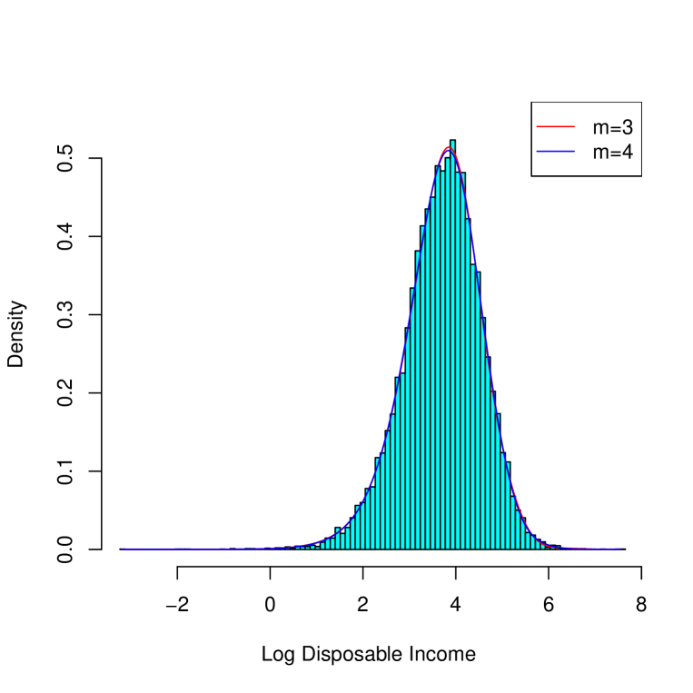
Figure 1: Histogram of log disposable income and density function of fitted log Gamma mixtures with order $m=3$ and $m=4$.

We fit a set of finite Gamma mixture models with a structural shape parameter $r$ and order $m=1,2,\dots,7$. When $m$ is greater than 2, we first used 50 random initial values to drive the EM algorithm and obtained up to 50 local maxima of the likelihood function. We took the local maximum with the highest likelihood value as the tentative MLE. Next, we created 10 initial values by perturbing the tentative MLE and generated a further 19 randomly. When the EM iteration stopped, we selected the estimate with the highest $\ell_{n}$ value as the MLE. For numerical stability, we adopted the modified likelihood with $\epsilon=0.001$. Table 4 gives the MLEs and corresponding likelihood values. By the nature of the maximum likelihood, $\ell_{n}(\hat{G})$ increases as the order $m$ of the mixture models increases. The size of the increment stalls at $m=7$.

Figure 2 gives a QQ-plot for the fitted Gamma mixture models (log transformed), together with the 45-degree line. The data points nearly perfectly align with the straight line when $m=3$ and $4$. There is practically no room for further improvement by increasing $m$.

With a structural shape parameter $r$, the number of parameters in the finite Gamma mixture model does not increase as quickly with $m$. Although the mixture model is not regular, the Bayes information criterion still provides some guidance. For the current sample size, a higher order of mixture model will be recommended when the log-likelihood is increased by 40. With this general guidance, a finite Gamma mixture of order $m=3$ is recommended; $m=4$ is also acceptable.

The fitted finite Gamma mixture distribution of order $m=3$ suggests that about 75% of the households have a low mean annual disposable income of $19,000$ yuan. A small percentage, 0.3%, of the households have 10 times this value. Setting $m=4$ changes the picture of the low and medium-income households only slightly. However, it separates a much smaller percentage, 0.04%, of super-rich households. They have nearly 30 times the mean income of the low-income households.

Table 4: MLEs of Gamma mixtures for disposable income

$m$	$1$	$2$	$3$	$4$	$5$	$6$	$7$
$\hat{r}$	1.6945	2.0261	2.1841	2.2433	2.3293	2.3526	2.4391
$\hat{\alpha}_{1}$		0.9129	0.7436	0.6009	0.0008	0.0002	0.0002
$\hat{\alpha}_{2}$		0.0871	0.2531	0.3740	0.5486	0.0008	0.0009
$\hat{\alpha}_{3}$			0.0033	0.0247	0.4214	0.5363	0.0094
$\hat{\alpha}_{4}$				0.0004	0.0288	0.4323	0.5311
$\hat{\alpha}_{5}$					0.0004	0.0300	0.4280
$\hat{\alpha}_{6}$						0.0004	0.0301
$\hat{\alpha}_{7}$							0.0004
$\hat{\theta}_{1}$	32.876	23.744	19.290	17.189	0.2408	0.0526	0.0509
$\hat{\theta}_{2}$		66.805	41.620	33.102	15.714	0.4046	0.4037
$\hat{\theta}_{3}$			190.82	78.326	30.811	15.353	5.0650
$\hat{\theta}_{4}$				484.69	73.740	30.271	14.804
$\hat{\theta}_{5}$					466.97	72.579	29.496
$\hat{\theta}_{6}$						462.15	70.756
$\hat{\theta}_{7}$							449.30
$\ell_{n}$	-84,911	-84,542	-84,487	-84,478	-84,468	-84,467	-84,467

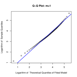
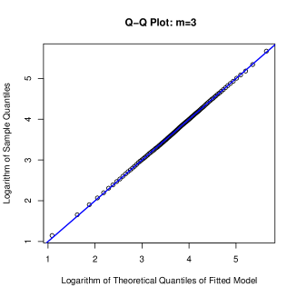
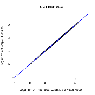
Figure 2: QQ plots of fitted gamma mixtures.

7 Discussion and observations

The finite Gamma mixture distributions are useful for modeling positive data that is suspected to come from a heterogeneous population. However, the MLE of the general Gamma mixture model is inconsistent. We have shown that the MLE of the finite Gamma mixture model with a structural shape parameter is strongly consistent. The simulation results indicate that the MLE has respectable finite-sample properties and observable consistency trends. The real-data example demonstrates that this model is able to reveal potential subpopulation structure.

References

- Chen and Chen [2003] Chen, H., Chen, J., 2003. Tests for homogeneity in normal mixtures in the presence of a structural parameter. Statistica Sinica 13, 351–365.
- Chen [1998] Chen, J., 1998. Penalized likelihood-ratio test for finite mixture models with multinomial observations. The Canadian Journal of Statistics 26, 583–599.
- Chen [2017] Chen, J., 2017. Consistency of the MLE under mixture models. Statistical Science 32, 47–63.
- Chen et al. [2016] Chen, J., Li, S., Tan, X., 2016. Consistency of the penalized MLE for two-parameter gamma mixture models. Science China Mathematics 59, 2301–2318.
- Chen and Tan [2009] Chen, J., Tan, X., 2009. Inference for multivariate normal mixtures. J. Multivar. Anal. 100, 1367–1383. doi:10.1016/j.jmva.2008.12.005.
- Chen et al. [2008] Chen, J., Tan, X., Zhang, R., 2008. Inference for normal mixtures in mean and variance. Statistica Sinica 18, 443–465.
- CHIP13 [2016] CHIP13, 2016. Chinese household income and expenditure project. http://www.ciidbnu.org/chip/chips.asp?year=2013.
- Ciuperca et al. [2003] Ciuperca, G., Ridolfi, A., Idier, J., 2003. Penalized maximum likelihood estimator for normal mixtures. Scandinavian Journal of Statistics 30, 45–59.
- Dempster et al. [1977] Dempster, A.P., Laird, N.M., Rubin, D.B., 1977. Maximum likelihood from incomplete data via the EM algorithm. Journal of the Royal Statistical Society, Series B 39, 1–38.
- Hathaway [1985] Hathaway, R.J., 1985. A constrained formulation of maximum-likelihood estimation for normal mixture distributions. The Annals of Statistics 13, 795–800.