State-independent quantum contextuality with projectors of nonunit rank

Abstract

Virtually all of the analysis of quantum contextuality is restricted to the case where events are represented by rank-one projectors. This restriction is arbitrary and not motivated by physical considerations. We show here that loosening the rank constraint opens a new realm of quantum contextuality and we demonstrate that state-independent contextuality can even require projectors of nonunit rank. This enables the possibility of state-independent contextuality with less than 13 projectors, which is the established minimum for the case of rank one. We prove that for any rank, at least 9 projectors are required. Furthermore, in an exhaustive numerical search we find that 13 projectors are also minimal for the cases where all projectors are uniformly of rank two or uniformly of rank three.

I Introduction

Experiments provide strong evidence that the measurements on quantum systems cannot be reproduced by any noncontextual hidden variable model (NCHV). In a NCHV model each outcome of any measurement has a preassigned value and this value in particular does not depend on which other properties are obtained alongside. This phenomenon is called quantum contextuality. Being closely connected to the incompatibility of observables [1], quantum contextuality is the underlying feature of quantum theory that enables, for example, the violation of Bell inequalities [2], enhanced quantum communication [3, 4], cryptographic protocols [5, 6], quantum enhanced computation [7, 8], and quantum key distribution [9].

The first example of quantum contextuality was found by Kochen and Specker [10] and requires 117 rank-one projectors. Subsequently the number of projectors was reduced until it was proved that the minimal set has 18 rank-one projectors [11]. This analysis was based on the particular type of contradiction between value assignments and projectors that was already used in the original proof by Kochen and Specker. The situation changed with the introduction of state-independent noncontextuality inequalities, where any NCHV model obeys the inequality, while it is violated for any quantum state and a certain set of projectors. With this enhanced definition of state-independent contextuality (SIC), Yu and Oh [12] found an instance of SIC with only 13 rank-one projectors and subsequently it was proved that this set is minimal [13] provided that all projectors are of rank one. Note that the iconic example of the Peres–Mermin square [14, 15] uses 9 observables with two-fold degenerate eigenspaces, but they are combined to 6 measurements of 24 rank-one projectors.

In contrast, SIC involving nonunit rank projectors has been rarely considered. To the best of our knowledge, the only examples [16, 15, 17, 18] which use nonunit rank are based on the Mermin star [19]. In these examples it was shown that nonunit projectors are sufficient for SIC, but it was not shown whether nonunit projectors are also necessary for SIC. Furthermore, in a graph theoretical analysis by Ramanathan and Horodecki [20] a necessary condition for SIC was provided which also allows one to study the case of nonunit rank.

In this article, we develop mathematical tools to analyze SIC for the case of nonunit rank. We first show that in certain situations nonunit rank is necessary for SIC. Then we approach the question whether projectors with nonunit rank enable SIC with less than 13 projectors. We find that in this case at least 9 projectors are required. For the special cases of SIC where all projectors are of rank 2 or rank 3 we find strong numerical evidence that 13 is indeed the minimal number of projectors.

This paper is structured as follows. In Section II we give an introduction to quantum contextuality using the graph theoretic approach. We extend this discussion to SIC in Section III and we give an example where rank-two projectors are necessary for SIC. In Section IV we provide a general analysis of the case of nonunit rank and show that scenarios with 8 or less projectors do not feature SIC, irrespective of the involved ranks. This analysis is used in Section V to show in an exhaustive numerical search that all graphs smaller than the graph given by Yu and Oh do not have SIC, if the rank of all projectors is 2 or 3. We conclude in Section VI with a discussion of our results.

II Contextuality and the graph theoretic approach

Our analysis is based on the graph theoretic approach to quantum contextuality [21]. In this approach an exclusivity graph $G$ with vertices $V(G)$ and edges $E(G)$ specifies the exclusivity relations in a contextuality scenario. The vertices represent events and two events are exclusive if they are connected by an edge. The cliques of the graph form the contexts of the scenario. (In Appendix A we give definitions of essential terms from graph theory.) Recall that an event is a class of outcomes in an experiment and two events are exclusive if they cannot be obtained simultaneously in any experiment. We consider now two types of models implementing the exclusivity graph, quantum models and noncontextual hidden variable models.

In a quantum model of the exclusivity graph $G$ one assigns projectors $\Pi_{k}$ to each event $k$ such that $\sum_{k\in C}\Pi_{k}$ is again a projector for every context $C$. This is equivalent to having $\Pi_{k}\Pi_{l}=0$ for any two exclusive events $k$ and $l$. With such an assignment and a quantum state $\rho$ one obtains the probability for the event $k$ as

$$P_{\mathrm{QT}}(k)=\operatorname{tr}(\rho\Pi_{k}).$$ (1)

The set of all probability assignments $P_{\mathrm{QT}}$ that can be reached with some projectors $(\Pi_{k})_{k}$ and some state $\rho$ is a convex set which coincides[21] with the theta body $\operatorname{TH}(G)$ of the graph $G$.

In contrast, in a NCHV model for the exclusivity graph $G$ the events are predetermined by a hidden variable $\lambda\in\Lambda$. That is, to each event $k$ one associates a response function $R_{k}\colon\Lambda\to\set{0,1}$. For a context $C$ the function $\lambda\mapsto\sum_{k\in C}R_{k}(\lambda)$ has to be again a response function, which is equivalent to $R_{k}(\lambda)R_{l}(\lambda)=0$ for all $\lambda$ and any pair of exclusive events $k$ and $l$. The probability of an event $k$ is now given by

$$P_{\mathrm{NCHV}}(k)=\sum_{\lambda\in\Lambda}\mu(\lambda)R_{k}(\lambda),$$ (2)

where $\mu$ is some probability distribution over the hidden variable space $\Lambda$. The set of all probability assignments $P_{\mathrm{NCHV}}$ that can be reached with some response functions $(R_{k})_{k}$ and some distribution $\mu$ forms a polytope which can be shown [21] to be the stable set $\operatorname{STAB}(G)$ of the graph $G$.

Quantum models and NCHV models are both noncontextual in the sense that the computation of the probability $P(k)$ of an event $k$ does not depend on the context in which $k$ is contained. Quantum contextuality occurs now for an exclusivity graph $G$ if we can find a quantum model with probability assignment $P_{\mathrm{QT}}$ which cannot be achieved by any NCHV model and hence $P_{\mathrm{QT}}\in\operatorname{TH}(G)\setminus\operatorname{STAB}(G)$. Since $\operatorname{STAB}(G)$ is convex, it is possible to find nonnegative numbers $(w_{k})_{k\in V(G)}\equiv\mathbf{w}$ such that

$$I_{\mathbf{w}}\colon P\mapsto\sum_{k}w_{k}P(k)$$ (3)

separates all NCHV models from some of the quantum models. That is, there exists some $\alpha$, such that $I_{\mathbf{w}}(P_{\mathrm{NCHV}})\leq\alpha$ holds for any $P_{\mathrm{NCHV}}\in\operatorname{STAB}(G)$, while $I_{\mathbf{w}}(P_{\mathrm{QT}})>\alpha$ holds true for some $P_{\mathrm{QT}}\in\operatorname{TH}(G)$. This can be further formalized by realizing that the weighted independence number [22] $\alpha(G,\mathbf{w})$ is exactly the maximal value that $I_{\mathbf{w}}$ attains within $\operatorname{STAB}(G)$ and similarly that the weighted Lovász number [23] $\vartheta(G,\mathbf{w})$ is exactly the maximum of $I_{\mathbf{w}}$ over $\operatorname{TH}(G)$. Consequently the inequality $I_{\mathbf{w}}(P_{\mathrm{NCHV}})\leq\alpha(G,\mathbf{w})$ holds for all NCHV probability assignments and this inequality is violated by some quantum probability assignment if and only if [21] $\vartheta(G,\mathbf{w})>\alpha(G,\mathbf{w})$ holds. In addition, one can show [21] that the value of $\vartheta(G,\mathbf{w})$ can always be attained for some quantum model employing only rank-one projectors.

III State-independent contextuality and nonunit rank

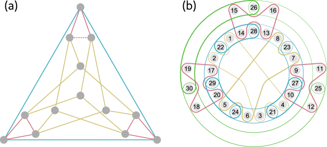
Figure 1: (a) The graph $G_{\mathrm{YO}}$ with 13 vertices and 24 edges. Removing the dashed edge yields the graph $G^{\prime}_{\mathrm{YO}}$. (b) Representation of the graph $G_{\mathrm{Toh}}$. Any subset of the vertices $1,2,\dotsc,30$ enclosed by a line forms a clique, that is, all vertices in any of the sets $\set{1,2,3,4}$, $\set{5,6,7,8}$, $\set{9,10,11,12}$, $\set{13,14,15,16}$, $\set{17,18,19,20}$, $\set{28,14,1,22}$, $\set{22,2,17,29}$, $\set{29,20,5,24}$, $\set{24,6,3,21}$, $\set{21,4,10,27}$, $\set{27,9,7,23}$, $\set{23,8,13,28}$, $\set{26,15,19,30}$, $\set{30,18,12,25}$, or $\set{25,11,16,26}$ are mutually connected by an edge.

The discussion so far concerns quantum models as being specified by the projectors assigned to each event together with a quantum state. In SIC one removes the quantum state from the specification of a quantum model and instead requires that probabilities from the quantum model cannot be reproduced by a NCHV model, independent of the quantum state. Therefore we consider the set of probability assignments formed by all quantum states and fixed projectors $(\Pi_{k})_{k}$,

$$\mathcal{P}_{\mathrm{SIC}}=\set{P\colon k\mapsto\operatorname{tr}(\rho\Pi_{k})}{\rho\text{ is a quantum state}}.$$ (4)

This set is also convex, since $P$ is linear and the set of quantum states is convex. Hence, in the case of SIC it is again possible to find nonnegative numbers $(w_{k})_{k}\equiv\mathbf{w}$ such that $I_{\mathbf{w}}$ separates $\operatorname{STAB}(G)$ from $\mathcal{P}_{\mathrm{SIC}}$. Therefore, it holds that

$$\sum_{k}w_{k}\operatorname{tr}(\rho\Pi_{k})>\alpha(G,\mathbf{w}),\text{ for all }\rho,$$ (5)

or, equivalently, that the eigenvalues of

$$\sum_{k}w_{k}\Pi_{k}-\alpha(G,\mathbf{w})$$ (6)

are all strictly positive.

We say that the projectors $(\Pi_{k})_{k}$ of a quantum model of $G$ form a rank-$\mathbf{r}$ projective representation of $G$, when $\mathbf{r}=(r_{k})_{k\in V(G)}$ with $r_{k}$ the rank of $\Pi_{k}$. The smallest known contextuality scenario which allows SIC is given by the exclusivity graph $G_{\mathrm{YO}}$ with 13 vertices [12]. This graph is shown in Figure 1 (a). For this scenario it is sufficient to consider rank-one projective representations. It also has been shown that no exclusivity graph with 12 or less vertices allows SIC [13], provided that all projectors are of rank one, $\mathbf{r}=\mathbf{1}$. But this does not yet show that SIC requires 13 projectors, since it is possible that a contextuality scenario features SIC only if some of the projectors are of nonunit rank.

This rises the question whether projectors of nonunit rank can be of advantage regarding SIC. We now show that this is the case by analyzing the exclusivity graph $G_{\mathrm{Toh}}$ with 30 vertices [18]. This graph is shown in Figure 1 (b). One can find a rank-two projective representation of this graph [18], such that $\sum_{k}\Pi_{k}=7+\frac{1}{2}$. Since the independence number of $G_{\mathrm{Toh}}$ is $7$, that is, $\alpha(G_{\mathrm{Toh}})\equiv\alpha(G_{\mathrm{Toh}},\mathbf{1})=7$, this shows that rank two is sufficient for SIC in this scenario.

For necessity, we show that no rank-one projective representation featuring SIC of $G_{\mathrm{Toh}}$ exists. We first note that such a representation would be necessarily constructed in a four-dimensional Hilbert space. This is the case because the largest clique of $G_{\mathrm{Toh}}$ has size four and hence any projective representation must contain at least four mutually orthogonal projectors of rank one. For an upper bound on the dimension $d$ of any projective representation featuring SIC we use the result [20, 24]

$$d<\chi_{\mathrm{f}}(G),$$ (7)

where $\chi_{\mathrm{f}}(G)$ denotes the fractional chromatic number of $G$. One finds $\chi_{\mathrm{f}}(G_{\mathrm{Toh}})=4+\frac{2}{7}$ implying $d\leq 4$. We do not find any rank-one projective representation of $G_{\mathrm{Toh}}$ in dimension $d=4$ using the numerical methods discussed in Section V.2 and in Appendix B we prove also analytically that no such representation exists.

IV Graph approach for projective representations of arbitrary rank

The example of the previous section showed that considering projective representations of nonunit rank can be necessary for the existence of a quantum model with SIC. Since the case of rank-one has already been analyzed in detail, it is helpful to reduce the case of nonunit rank to the case of rank one. To this end we adapt the notation [25] $G^{\mathbf{r}}$ for the graph where each vertex $k$ is replaced by a clique $C_{k}$ of size $r_{k}$ and all vertices between two cliques $C_{k}$ and $C_{\ell}$ are connected when $[k,\ell]$ is an edge. See Figure 2 for an illustration. That is,

$$V(G^{\mathbf{r}}) =\set{(k,i)}{k\in V(G),\;i=1,2,\dotsc,r_{k}},$$ (8)

$$E(G^{\mathbf{r}}) =\set{[(k,i),(\ell,j)]}{[k,\ell]\in E(G)\text{ or }(k=\ell\text{ and }i\neq j)}.$$ (9)

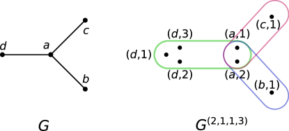
Figure 2: Illustration of the graph $G^{\mathbf{r}}$. $G$ has vertices $a,b,c,d$ and here $r_{a}=2$, $r_{b}=1$, $r_{c}=1$, $r_{d}=3$. In the product graph, vertices enclosed by a line form a clique, that is, they are all mutually connected by an edge.

The construction of $G^{\mathbf{r}}$ is such that if $(\Pi_{k,i})_{k,i}$ is a rank-one projective representation of $G^{\mathbf{r}}$, then evidently $\Pi_{k}=\sum_{i}\Pi_{k,i}$ defines a rank-$\mathbf{r}$ projective representation of $G$. Vice versa, if $(\Pi_{k})_{k}$ is a rank-$\mathbf{r}$ projective representation of $G$, then one can immediately construct a rank-one projective representation of $G^{\mathbf{r}}$ by decomposing each projector $\Pi_{k}$ into rank-one projectors $(\Pi_{k,i})_{i}$ such that $\Pi_{k}=\sum_{i}\Pi_{k,i}$.

For a given graph $G$ we denote by $d_{\pi}(G,\mathbf{r})$ the minimal dimension which admits a rank-$\mathbf{r}$ projective representation and by $\chi_{\mathrm{f}}(G,\mathbf{r})$ the fractional chromatic number for the graph $G$ with vertex weights $\mathbf{r}\in\mathbb{N}^{\lvert V(G)\rvert}$. In addition we abbreviate the Lovász function of the complement graph by $\overline{\vartheta}(G,\mathbf{r})=\vartheta(\overline{G},\mathbf{r})$. For these three functions we omit the second argument if $r_{k}=1$ for all $k$, that is, $\chi_{\mathrm{f}}(G)\equiv\chi_{\mathrm{f}}(G,\mathbf{1})$, etc.

Theorem 1.

For any graph $G$ and vertex weights $\mathbf{r}\in\mathbb{N}^{\lvert V(G)\rvert}$ we have $d_{\pi}(G^{\mathbf{r}})=d_{\pi}(G,\mathbf{r})$, $\chi_{\mathrm{f}}(G^{\mathbf{r}})=\chi_{\mathrm{f}}(G,\mathbf{r})$, and $\overline{\vartheta}(G^{\mathbf{r}})=\overline{\vartheta}(G,\mathbf{r})$. In addition, $\chi_{\mathrm{f}}(G,m\mathbf{r})=m\chi_{\mathrm{f}}(G,\mathbf{r})$ and $\overline{\vartheta}(G,m\mathbf{r})=m\overline{\vartheta}(G,\mathbf{r})$ hold for any $m\in\mathbb{N}$.

The proof is provided in Appendix C. As a consequence we extend the relation [23] $\overline{\vartheta}(G)\leq d_{\pi}(G)$ (see also Appendix A) to the case of nonunit rank,

$$\overline{\vartheta}(G,\mathbf{r})\leq d_{\pi}(G,\mathbf{r}).$$ (10)

Similarly we have generalization of the condition in Eq. (7): Whenever a graph $G$ has a rank-$\mathbf{r}$ projective representation featuring SIC, then it holds that

$$d_{\pi}(G,\mathbf{r})<\chi_{\mathrm{f}}(G,\mathbf{r}).$$ (11)

Following the ideas from Refs. 20, 26, we consider quantum models that use the maximally mixed state $\rho_{\mathrm{mm}}=\openone/d$, where $d$ is the dimension of the Hilbert space. For a rank-$\mathbf{r}$ projective representation, the corresponding probability assignment is then simply given by

$$P_{\mathrm{mm}}(k)=r_{k}/d.$$ (12)

If the representation features SIC, then $P_{\mathrm{mm}}\notin\operatorname{STAB}(G)$, since, by definition, $P_{\mathrm{mm}}\in\mathcal{P}_{\mathrm{SIC}}$ while $\mathcal{P}_{\mathrm{SIC}}$ and $\operatorname{STAB}(G)$ are disjoint sets. This is the motivation to define the set $\operatorname{RANK}(G)$ of all probability assignments $P_{\mathrm{mm}}$ which arise from any projective representation of $G$. That is,

$$\operatorname{RANK}(G)=\set{\mathbf{r}/\ell}{\mathbf{r}\in\mathbb{N}^{\lvert V(G)\rvert}\text{, }\ell\in\mathbb{N},\text{ such that }\ell\geq d_{\pi}(G,\mathbf{r})}.$$ (13)

Denoting by $\overline{\operatorname{RANK}}(G)$ the topological closure of $\operatorname{RANK}(G)$ we show in Appendix D the following inclusions.

Theorem 2.

For any graph $G$, the set $\overline{\operatorname{RANK}}(G)$ is convex and $\operatorname{STAB}(G)\subseteq\overline{\operatorname{RANK}}(G)\subseteq\operatorname{TH}(G)$.

This implies that any NCHV probability assignment can be arbitrarily well approximated by a quantum probability assignment using the maximally mixed state. Conversely, if $\operatorname{RANK}(G)\subset\operatorname{STAB}(G)$ for an exclusivity graph $G$, then any quantum probability assignment using the maximally mixed state can be reproduced by a NCHV model and hence no projective representation of $G$ can feature SIC. This is the case for all graphs with at most 8 vertices, as we show in Appendix E by using a linear relaxation of $\operatorname{RANK}(G)$.

Theorem 3.

$\operatorname{STAB}(G)=\overline{\operatorname{RANK}}(G)$ for any graph $G$ with $8$ vertices or less.

Since any exclusivity graph allowing SIC must have $\overline{\operatorname{RANK}}(G)\supsetneq\operatorname{STAB}(G)$, this implies the following statement.

Corollary 4.

Any scenario allowing SIC requires more than 8 events.

V Minimal State-Independent Contextuality

We now aim to find the smallest scenario allowing SIC, that is, the smallest exclusivity graph which has a projective representation featuring SIC. Here, we say that a graph $G^{\prime}$ is smaller than a graph $G$ if either $G^{\prime}$ has less vertices than $G$ or if both have the same number of vertices and $G^{\prime}$ has less edges than $G$. With this notion, the smallest known graph allowing SIC is $G^{\prime}_{\mathrm{YO}}$ with 13 vertices and 23 edges, where $G^{\prime}_{\mathrm{YO}}$ is $G_{\mathrm{YO}}$ but with one edge removed as shown in Figure 1 (a). Due to Corollary 4 it remains to consider the graphs with 9 and up to 12 vertices as well as all graphs with 13 vertices and 23 edges or less.

Instead of testing for a projective representation featuring SIC, we use the weaker condition in Eq. (11) and we limit our considerations to rank-$r$ representations where all projectors have the same rank and $r=1$, $r=2$, or $r=3$. We now aim to establish the following.

Assertion 5.

For $r=1,2,3$, the smallest graph $G$ with $d_{\pi}(G,r\mathbf{1})<\chi_{\mathrm{f}}(G,r\mathbf{1})$ is $G^{\prime}_{\mathrm{YO}}$.

This assertion implies that $G^{\prime}_{\mathrm{YO}}$ is the smallest graph admitting SIC when considering rank-$r$ projective representations for $r=1,2,3$.

Our approach to Assertion 5 consists of two steps. First we identify four conditions that are easy to compute and necessary for $d_{\pi}(G,\mathbf{r})<\chi_{\mathrm{f}}(G,\mathbf{r})$ to hold. For graphs which satisfy all these conditions and for $\mathbf{r}=r\mathbf{1}$ with $r=1,2,3$, we then implement a numerical optimization algorithm in order to compute $d_{\pi}(G,r\mathbf{1})$. We then confirm Assertion 5, aside from the uncertainty that is due to the numerical optimization.

V.1 Conditions

We introduce four necessary conditions that are satisfied if $G$ is the smallest graph with $d_{\pi}(G,\mathbf{r})<\chi_{\mathrm{f}}(G,\mathbf{r})$ for some fixed $\mathbf{r}$. First, we consider the case where $G$ is not connected. Then there exists a partition of the vertices $V(G)$ into disjoint subsets $V_{i}\subsetneq V(G)$ such that no two vertices from different subsets are connected. We write $G_{i}$ for the corresponding induced subgraph and similarly $\mathbf{r}_{i}$. It is easy to see (see Appendix A), that $d_{\pi}(G,\mathbf{r})=\max_{i}d_{\pi}(G_{i},\mathbf{r}_{i})$ and $\chi_{\mathrm{f}}(G,\mathbf{r})=\max_{i}\chi_{\mathrm{f}}(G_{i},\mathbf{r}_{i})$ and hence $d_{\pi}(G,\mathbf{r})<\chi_{\mathrm{f}}(G,\mathbf{r})$ implies that already $d_{\pi}(G_{i},\mathbf{r}_{i})<\chi_{\mathrm{f}}(G_{i},\mathbf{r}_{i})$ for some $i$. But this is at variance with the assumption that $G$ is minimal. Hence we have the following.  
 
Condition 1. $G$ is connected.

Second, we consider a partition of $V(G)$ into disjoint subset $V_{i}\subsetneq V(G)$ such that any two vertices from different subsets are connected. We have $d_{\pi}(G,\mathbf{r})=\sum_{i}d_{\pi}(G_{i},\mathbf{r}_{i})$ and $\chi_{\mathrm{f}}(G,\mathbf{r})=\sum_{i}\chi_{\mathrm{f}}(G_{i},\mathbf{r}_{i})$ (see Appendix A) and hence $d_{\pi}(G,\mathbf{r})<\chi_{\mathrm{f}}(G,\mathbf{r})$ implies $d_{\pi}(G_{i},\mathbf{r})<\chi_{\mathrm{f}}(G_{i},\mathbf{r})$ for some $i$ and thus $G$ is not minimal.  
 
Condition 2. $\overline{G}$ is connected.

Third, we write $G-e$ for the subgraph with the edge $e$ removed. Clearly, $d_{\pi}(G-e,\mathbf{r})\leq d_{\pi}(G,\mathbf{r})$. Thus, if $d_{\pi}(G,\mathbf{r})<\chi_{\mathrm{f}}(G,\mathbf{r})$ and $\chi_{\mathrm{f}}(G,\mathbf{r})=\chi_{\mathrm{f}}(G-e,\mathbf{r})$, then we have already $d_{\pi}(G-e,\mathbf{r})<\chi_{\mathrm{f}}(G-e,\mathbf{r})$ and $G$ cannot be minimal. In order to avoid this contradiction, we need the following.  
 
Condition 3. $\chi_{\mathrm{f}}(G,\mathbf{r})\neq\chi_{\mathrm{f}}(G-e,\mathbf{r})$ for all edges $e$.

Note that if $\mathbf{r}=r\mathbf{1}$, then this condition reduces to $r\chi_{\mathrm{f}}(G)\neq r\chi_{\mathrm{f}}(G-e)$ and is independent of $r$. We can further sharpen Condition 3 by assuming merely $\lceil\chi_{\mathrm{f}}(G,\mathbf{r})\rceil=\lceil\chi_{\mathrm{f}}(G-e,\mathbf{r})\rceil$, where $\lceil x\rceil$ denotes the least integer not smaller than $x$. Then $d_{\pi}(G,\mathbf{r})<\chi_{\mathrm{f}}(G,\mathbf{r})$ implies $d_{\pi}(G-e,\mathbf{r})<\lceil\chi_{\mathrm{f}}(G-e,\mathbf{r})\rceil$ and since $d_{\pi}(G-e,\mathbf{r})$ is an integer, this also implies $d_{\pi}(G-e,\mathbf{r})<\chi_{\mathrm{f}}(G-e,\mathbf{r})$.  
 
Condition 4. $\lceil\chi_{\mathrm{f}}(G,\mathbf{r})\rceil\neq\lceil\chi_{\mathrm{f}}(G-e,\mathbf{r})\rceil$ for all edges $e$.

Finally, from Eq. (10) we have $\overline{\vartheta}(G,\mathbf{r})\leq d_{\pi}(G,\mathbf{r})$ and since $d_{\pi}(G,\mathbf{r})$ is an integer, we also have $\lceil\,\overline{\vartheta}(G,\mathbf{r})\rceil\leq d_{\pi}(G,\mathbf{r})$. This implies our last condition.  
 
Condition 5. $\lceil\,\overline{\vartheta}(G,\mathbf{r})\rceil<\chi_{\mathrm{f}}(G,\mathbf{r})$.

We apply these five conditions to all graphs with $n=9,10,11,12$ vertices and all graphs with $n=13$ vertices and 23 or less edges. The resulting numbers of graphs are listed in Table 1. First, all nonisomorphic graphs are generated using the software package “nauty” [27], where then all graphs violating Condition 1 or Condition 2 are discarded. Subsequently, Condition 3 is implemented and for the remaining graphs, $\overline{\vartheta}(G)$, $\chi_{\mathrm{f}}(G)$, and $\min_{e}\chi_{\mathrm{f}}(G-e)$ are computed, which then allows us to evaluate Condition 4 and Condition 5 for $\mathbf{r}=r\mathbf{1}$ with $r=1,2,3$.

For the computation of $\chi_{\mathrm{f}}$, we use a floating point solver for the corresponding linear program. On the basis of the solution of the program, an exact fractional solution is guessed and then verified using the strong duality of linear optimization. The Lovász number $\vartheta$ is computed by means of a floating point solver for the corresponding semidefinite program. The dual and primal solutions are verified and the gap between both is used to obtain a strict upper bound on the numerical error. This error is in practice of the order of $10^{-10}$ or better for the vast majority of the graphs.

rank	Condition	$n=9$	$n=10$	$n=11$	$n=12$	$n=13^{*}$
any	none	$274\,668$	$12\,005\,168$	$1\,018\,997\,864$	$165\,091\,172\,592$	$10\,951\,875\,086$
any	1 & 2	$247\,492$	$11\,427\,974$	$994\,403\,266$	$163\,028\,488\,360$	$9\,185\,079\,351$
$\mathbf{r}=r\mathbf{1}$	1–3	$52$	$608$	$13\,716$	$609\,373$	$16\,893$
$r=1$	1–4	$37$	$283$	$5\,122$	$163\,127$	$15\,596$
$r=1$	1–5	$1$	$11$	$446$	$31\,049$	$77$
$r=2$	1–4	$44$	$398$	$7\,159$	$238\,478$	$15\,691$
$r=2$	1–5	$8$	$126$	$2\,483$	$106\,400$	$172$
$r=3$	1–4	$45$	$430$	$8\,240$	$265\,346$	$15\,865$
$r=3$	1–5	$13$	$158$	$3\,574$	$133\,268$	$346$

Table 1: Numbers of graphs satisfying Condition 1–5. Condition 1–5 are applied to all graphs with $n$ vertices. For $n=13^{*}$ vertices, only the graphs with up to 23 edges are considered. Condition 3 can be applied for the case $\mathbf{r}=r\mathbf{1}$ for any $r$ but Condition 4 and Condition 5 are evaluated only for the cases $r=1,2,3$.

V.2 Numerical estimate of the dimension

If an exclusivity graph $G$ has a rank-$\mathbf{r}$ projective representation with SIC, then, according to Theorem 1 and the subsequent discussion, there must be a rank-one projective representation of $G^{\mathbf{r}}$ in dimension $d=\lceil\chi_{\mathrm{f}}(G,\mathbf{r})\rceil-1$. At this point, we do not further exploit the structure of the problem. We rather consider methods which allow us to verify or falsify the existence of a rank-one projective representation in dimension $d$ of an arbitrary graph $G$ with $n$ vertices.

If such a projective representation exists, then one can assign normalized vectors $\mathbf{y}_{k}\in\mathbb{C}^{d}$ to each vertex $k\in V(G)$ such that $\mathbf{y}_{\ell}^{\dagger}\mathbf{y}_{k}=0$ for all edges $[\ell,k]\in E(G)$. Collecting these vectors in the columns of a matrix $Y$, we obtain the feasibility problem

$$\begin{array}[]{lcl}\text{find}&&X=Y^{\dagger}Y\text{ with }Y\in\mathbb{C}^{d\times n},\\ \text{subject to}&&X_{k,k}=1\text{ for all }j\in V(G),\\ &&X_{\ell,k}=0\text{ for all }[\ell,k]\in E(G).\\ \end{array}$$ (14)

This problem is equivalent to the optimization problem

$$\begin{array}[]{lcl}\text{minimize}&&\sum_{k\in V(G)}(X_{k,k}-1)^{2}+\sum_{[\ell,k]\in E(G)}X_{\ell,k}^{2},\\ \text{with}&&X=Y^{\dagger}Y\text{ and }Y\in\mathbb{C}^{d\times n},\end{array}$$ (15)

where the problem in Eq. (14) is feasible if and only if the problem in Eq. (15) yields zero. The optimization can be executed using a standard algorithm like the conjugate-gradient method [28]. However, the obtained value can be from a local minimum and depend on the initial value used in the optimization. Hence obtaining a value greater than zero does not conclusively exclude the existence of a projective representation, but this problem can be mitigated by performing the minimization for many different initial values.

Instead of employing one of the standard optimization algorithms, we use a faster method that allows us to repeat the minimization with many different initial values. For this we denote by $\mathcal{L}$ the set of all $(n\times n)$-matrices $X$ which satisfy the constraints of the problem in Eq. (14) and we write $\mathcal{R}$ for the set of all matrices $X$ for which $X=Y^{\dagger}Y$ for some $(d\times n)$-matrix $Y$. In an alternating optimization, we generate a sequence $(X^{(j)})_{j}$ from an initial value $X^{(0)}$ such that

$$\begin{split}X^{(2i+1)}&=\operatorname{arg~{}min}_{R}\set{\lVert R-X^{(2i)}\rVert}{R\in\mathcal{R}},\\ X^{(2i)}&=\operatorname{arg~{}min}_{L}\set{\lVert L-X^{(2i-1)}\rVert}{L\in\mathcal{L}}.\end{split}$$ (16)

By construction, $\delta_{j}=\lVert X^{(j)}-X^{(j-1)}\rVert$ is a nonincreasing sequence and hence $\delta_{\infty}=\lim_{j\to\infty}\delta_{j}$ exists. Consequently, for the existence of a projective representation it is sufficient if $\delta_{\infty}=0$ because then $X^{(\infty)}=\lim_{j\to\infty}X^{(j)}$ exists with $X^{(\infty)}\in\mathcal{R}\cap\mathcal{L}$. In Appendix F we show that this alternating optimization can be implemented efficiently for the Frobenius norm $\lVert M\rVert_{F}=\sum_{i,j}\lvert M_{i,j}\rvert^{2}$.

We run the optimization with $100$ randomly chosen initial values $X^{(0)}$ for each of the remaining graphs with corresponding rank $r$. We stop the optimization if $\delta_{k-2}/\delta_{k}<1+10^{-5}$. For all graphs and all repetitions the optimization converges with a final value of $\delta_{k}$ in the order of $1$. In comparison, we test the algorithm for many graphs with known $d_{\pi}$ where the graphs have up to 40 vertices. In all these cases, the algorithm converges to $\delta_{k}$ in the order of $10^{-9}$, which gives us confidence that the alternating optimization is reliable. In summary this constitutes strong numerical evidence that none of the remaining graphs with corresponding rank has a projective representation with SIC.

VI Conclusion and discussion

The search for a primitive entity of contextuality has not yet reached a conclusion despite of decades of research on this topic. Of course, one can argue that the pentagon scenario by Klyachko et al. [29] does provide a provably minimal scenario. But the drawback of the pentagon scenario is that it is state-dependent. That is, contextuality is here a feature of both, the state and the measurements. In contrast, in the state-independent approach, contextuality is a feature exclusively of the measurements and we argue that a primitive entity of contextuality should embrace state-independence. Among the known SIC scenarios, the one by Yu and Oh [12] is minimal and this has also been proved rigorously for the case where all measurement outcomes are represented by rank-one projectors.

As we pointed out here, there is no guarantee that the actual minimal scenario will also be of rank one: We showed that a scenario by Toh[18]—albeit far from minimal—requires projectors of rank two. This motivated our search for the minimal SIC scenario for the case of nonunit rank. Due to Theorem 3, we can exclude the case where the exclusivity graph has 8 or less vertices. For the remaining cases of 9 to 12 vertices, we also obtain a negative result, however, under the restriction that the projective representation is uniformly of rank two or uniformly of rank three. A key to this result is a fast and empirically reliable numerical method to find or exclude projective representations of a graph, which might be also a useful method for related problems in graph theory.

Curiously, there is no simple argument that shows that the scenario by Yu and Oh is minimal, even when assuming unit rank. This in contrast to the case of state-dependent contextuality, where the reason that the pentagon scenario is the simplest scenario beautifully has the origin in graph theory[21]. For the future it will be interesting to develop additional methods for SIC, in particular for the case of heterogeneous rank. It will be particularly interesting whether this problem can be solved using more methods from graph theory, whether it can be solved using new numerical methods, or whether the problem turns out to be genuinely hard to decide.

Appendix A Elements from graph theory

A graph $G$ is a collection of vertices $V(G)$ connected by edges $E(G)$. Each edge $[i,j]\in$ is an unordered pair of the vertices $i\neq j\in V(G)$. Conversely, for a given vertex set $V$ and edge set $E$ the pair $(V,E)$ forms the graph denoted by $G(V,E)$. For a given subset $W$ of $V$ and subset $F$ of $E$, the graph $G(W,F)$ is a subgraph of $G(V,E)$. In the case where

$$F=E\cap\{[i,j]\}_{i,j\in W},$$ (17)

$G(W,F)$ is a subgraph of $G(V,E)$ induced by the subset $W$. In the case where

$$F=\{[i_{t},i_{t+1}]\}_{t},$$ (18)

$G(W,F)$ is a path in $G(V,E)$. A graph $G(V,E)$ is connected if any two vertices can be connected by a path. A subset of vertices $C$ is a clique, if in the induced subgraph all vertices are mutually connected by an edge. A clique $C$ is maximal, if any strict superset of $C$ is not clique. The complement graph $\bar{G}$ of $G$ has an edge $[i,j]$ if and only if $i\neq j$ and $[i,j]$ is not an edge in $G$. A clique in $\bar{G}$ is an independent set of $G$. Independent sets are also called stable sets. If any strict superset of $W$ is not an independent set, then $W$ is a maximally independent set.

Now, the index vector of a given subset of vertices $W$ is defined as

$$\Delta_{W}=[\delta_{W}(k)]_{k\in V},$$ (19)

where $\delta_{W}(k)=1$ if $k\in W$ and $\delta_{W}(k)=0$ otherwise. Let $\mathcal{I}$ denote the set of all independent sets of graph $G$, then the stable set polytope $\operatorname{STAB}(G)$ is the convex hull of the set $\set{\Delta_{W}}{W\in\mathcal{I}}$.

A collection of real vectors $(\mathbf{v}_{i})_{i\in V}$ is an orthogonal representation (OR) of $G$, provided that $[i,j]\not\in E$ implies $\mathbf{v}_{i}\cdot\mathbf{v}_{j}=0$. The Lovász theta body of a given graph $G$ can be defined as [30]

$$\operatorname{TH}(G)=\set{[(\mathbf{s}\cdot\mathbf{v}_{i})^{2}]_{i\in V}}{(\mathbf{v}_{i})_{i\in V}\ \text{is an OR of }\overline{G}},$$ (20)

where $\mathbf{s}=(1,0,\ldots,0)$. We also use the following, equivalent definition of $\operatorname{TH}(G)$. A collection of projectors $(\Pi_{k})_{k\in V}$ (over a complex Hilbert space) is a projective representation (PR) of $G$ if $\Pi_{i}\Pi_{j}=0$ whenever $[i,j]\in E(G)$. Then, one can also write [21]

$$\operatorname{TH}(G)=\set{[\operatorname{tr}(\rho\Pi_{i})]_{i\in V}}{(\Pi_{i})_{i\in V}\ \text{is a PR of }G,\operatorname{tr}(\rho)=1,\rho\geq 0}.$$ (21)

Note that in the definition, the projectors might be of any rank.

For a vector $\mathbf{r}$ of nonnegative real numbers,

$$\alpha(G,\mathbf{r})=\max_{\mathbf{x}}\set{\mathbf{r}\cdot\mathbf{x}}{\mathbf{x}\in\operatorname{STAB}(G)}$$ (22)

is the weighted independence number [30] and the weighted Lovász number is given [31] by

$$\vartheta(G,\mathbf{r})=\max_{\mathbf{x}}\set{\mathbf{r}\cdot\mathbf{x}}{\mathbf{x}\in\operatorname{TH}(G)}.$$ (23)

For convenience, we write $\overline{\vartheta}(G,\mathbf{r})=\vartheta(\overline{G},\mathbf{r})$.

The weighted chromatic number $\chi(G,\mathbf{r})$ can be defined as[25]

$$\min_{(c_{I})_{I\in\mathcal{I}}} \sum_{I\in\mathcal{I}}c_{I},$$ (24)

such that $$\sum_{I\ni i}c_{I}\geq r_{i},\text{ for all }i\in V,$$

where $c_{I}$ are nonnegative integers. Equivalently, if $C=\chi(G,\mathbf{r})$, then there exists an $\mathbf{r}$-coloring of $G$ with $C$ colors, that is, $C$ is the minimal number of colors such that $r_{k}$ colors are assigned to each vertex $k$ and two vertices $i$ and $j$ do not share a common color if they are connected.

The weighted fractional chromatic number $\chi_{\mathrm{f}}(G,\mathbf{r})$ is a relaxation of the integer program in Eq. (24) to a linear program [25]

$$\min_{(x_{I})_{I\in\mathcal{I}}} \sum_{I\in\mathcal{I}}x_{I},$$ (25)

such that $$\sum_{I\ni i}x_{I}\geq r_{i},\text{ for all }i\in V,$$

where $x_{I}$ are now nonnegative real numbers. Being a linear program with rational coefficients, all $x_{I}$ can be chosen to be rational numbers and hence one can find a $b\in\mathbb{N}$ such that all $bx_{I}$ are integer. This yields the relation

$$\chi_{f}(G,\mathbf{r})=\min_{b\in\mathbb{N}}\frac{\chi(G,b\mathbf{r})}{b}.$$ (26)

Finally, we use $d_{\pi}(G,\mathbf{r})$ as defined in the main text, that is, $d_{\pi}(G,\mathbf{r})$ is the minimal dimension admitting a rank-$\mathbf{r}$ PR. We also omit the weights $\mathbf{r}$ for the functions $d_{\pi}$, $\chi_{\mathrm{f}}$, and $\overline{\vartheta}$, if $\mathbf{r}=\mathbf{1}$. We now show the known relation [23] $\overline{\vartheta}(G)\leq d_{\pi}(G)$, which is extended to the case of $\mathbf{r}=\mathbf{1}$ in Eq. (10) in the main text.

Lemma 6.

$\overline{\vartheta}(G)\leq d_{\pi}(G)$

Proof.

For a given $d$-dimensional rank-$1$ PR $(\Pi_{k})_{k}$ of $G$, a $d^{2}$-dimensional rank-$1$ PR $(P_{k})_{k}$ of $G$ can be constructed as

$$P_{k}=\Pi_{k}^{*}\otimes\Pi_{k},$$ (27)

where complex conjugation is with respect to some arbitrary, but fixed orthonormal basis $\ket{1},\ket{2},\dotsc,\ket{d}$. Using $\Psi=\sum_{j,l}\ket{jj}\!\bra{ll}$, we have $\operatorname{tr}(\Psi P_{k})=1$ and $\operatorname{tr}(\Psi)=d$.

We consider now an arbitrary rank-$1$ PR $(Q_{k})_{k}$ of $\overline{G}$ together with an arbitrary density operator $\rho$ acting on the same Hilbert space as the PR. Then $(P_{i}\otimes Q_{j})_{i,j}$ is a PR of $G\otimes\overline{G}$ and $(i,i)$ is connected with $(j,j)$ either within $G$ or within $\overline{G}$, for any two vertices $i\neq j$. Here $G\otimes K$ denotes the graph with vertices $V(G)\times V(K)$ and where $[(v,w),(v^{\prime},w^{\prime})]$ is an edge, if $[v,v^{\prime}]$ or $[w,w^{\prime}]$ is an edge.

Therefore, $\sum_{k}P_{k}\otimes Q_{k}\leq\openone$ and consequently,

$$d=\operatorname{tr}(\Psi\otimes\rho)\geq\sum_{k}\operatorname{tr}([\Psi\otimes\rho][P_{k}\otimes Q_{k}])=\sum_{k}\operatorname{tr}(\rho Q_{k}).$$ (28)

By virtue of Eq. (21) we obtain $\sum x_{i}\leq d$ for all $\mathbf{x}\in\operatorname{TH}(\overline{G})$, which then yields the desired inequality due to Eq. (23). ∎

The disjoint union $G=G_{1}\cup G_{2}$ of two graphs consists of the disjoint union of the vertices, $V(G)=V(G_{1})\uplus V(G_{2})$, and $[i,j]$ is an edge in $G$ if it is an edge in either $G_{1}$ or $G_{2}$. For Condition 1 in Section V.1 we use the following observation.

Lemma 7.

If $G=\bigcup_{i}G_{i}$, then $d_{\pi}(G,\mathbf{r})=\max_{i}d_{\pi}(G_{i},\mathbf{r}_{i})$ and $\chi_{f}(G,\mathbf{r})=\max_{i}\chi_{f}(G_{i},\mathbf{r}_{i})$, where $\mathbf{r}_{i}$ is the part of $\mathbf{r}$ for $G_{i}$.

Proof.

By definition, $d_{\pi}(G,\mathbf{r})\geq\max_{i}d_{\pi}(G_{i},\mathbf{r}_{i})$. Conversely, if $d=\max_{i}d_{\pi}(G_{i},\mathbf{r}_{i})$ then we can find a $d$-dimensional rank-$\mathbf{r}_{i}$ PR for each $G_{i}$. Since the subgraphs are mutually disjoined, these PRs jointly form already a $d$-dimensional rank-$\mathbf{r}$ PR of $G$. Thus $d\geq d_{\pi}(G,\mathbf{r})$.

For the fractional chromatic number, one first observes that $G^{\mathbf{r}}=\bigcup_{i}G_{i}^{\mathbf{r}_{i}}$. Hence the assertion reduces to $\chi_{\mathrm{f}}(\bigcup_{i}G_{i}^{\mathbf{r}_{i}})=\max_{i}\chi_{\mathrm{f}}(G_{i}^{\mathbf{r_{i}}})$, which is a well-known relation for disjoint unions of graphs [32]. ∎

The join $G=G_{1}+G_{2}$ of two graphs is similar to the disjoint union, however with an additional edge between any two vertices $[i,j]$ if $i\in V(G_{1})$ and $j\in V(G_{2})$. For Condition 2 in Section V.1 we use then the following observation.

Lemma 8.

If $G=\sum_{i}G_{i}$, then $d_{\pi}(G,\mathbf{r})=\sum_{i}d_{\pi}(G_{i},\mathbf{r}_{i})$ and $\chi_{f}(G,\mathbf{r})=\sum_{i}\chi_{f}(G_{i},\mathbf{r}_{i})$.

Proof.

For given $d_{i}$-dimensional rank-$\mathbf{r}_{i}$ PRs $(\Pi_{j})_{j\in V(G_{i})}$ of $G_{i}$, we define

$$P_{j,i}=\left(\bigoplus_{k<i}\mathbb{O}_{k}\right)\oplus\Pi_{j}\oplus\left(\bigoplus_{k>i}\mathbb{O}_{d_{k}}\right),$$ (29)

where $j\in G_{i}$ and $\mathbb{O}_{k}$ is the zero-operator acting on the space of the PR of $G_{k}$. This construction achieves that $((P_{j,i})_{j\in V(G_{i})})_{i}$ is a $(\sum_{i}d_{i})$-dimensional rank-$\mathbf{r}$ PR of $G$ and therefore $d_{\pi}(G,\mathbf{r})\leq\sum_{i}d_{\pi}(G_{i},\mathbf{r}_{i})$ holds. Conversely, from a given $d$-dimensional rank-$\mathbf{r}$ PR of $G$, we can deduce a $d_{i}$-dimensional rank-$\mathbf{r}_{i}$ PR of each $G_{i}$, where $d_{i}$ is the dimension of the subspace $S_{i}$ where $(\Pi_{j})_{j\in G_{i}}$ acts nontrivially. Since each of subspace $S_{i}$ is orthogonal to the other subspaces $S_{j}$, we obtain $d\geq\sum_{i}d_{i}\geq\sum_{i}d_{\pi}(G_{i},\mathbf{r}_{i})$.

For the fractional chromatic number, we note that $G^{\mathbf{r}}=\sum_{i}G_{i}^{\mathbf{r}_{i}}$ and since $\chi_{\mathrm{f}}$ is additive under the join of graphs [32], the assertion follows. ∎

Appendix B $G_{\mathrm{Toh}}$ has no rank-one projective representation

It can be verified numerically that there is no $4$-dimensional rank-$1$ PR of $G_{\rm Toh}$ with our numerical methods in Appendix F. Here, we give an analytical proof with the help of the computer algebra system Mathematica.

Since each (row) vector $\mathbf{v}$ corresponds to a rank-$1$ projector $P(\mathbf{v})=\mathbf{v}^{\dagger}\mathbf{v}/|\mathbf{v}|^{2}$, we can use vectors instead of projectors in the case of rank-$1$ PR. Also, two non-zero vectors $\mathbf{v}_{1}$ and $\mathbf{v}_{2}$ are called equal if $P(\mathbf{v}_{1})=P(\mathbf{v}_{2})$. For three independent vectors $\mathbf{v}_{1},\mathbf{v}_{2},\mathbf{v}_{3}$ in the $4$-dimensional Hilbert space, from Cramer’s rule we know that their common orthogonal vector is proportional to $\Lambda(\mathbf{v}_{1},\mathbf{v}_{2},\mathbf{v}_{3})=(\lambda_{1},\lambda_{2},\lambda_{3},\lambda_{4})^{*}$, with $\mathbf{v}_{i}=\{v_{i,1},v_{i,2},v_{i,3},v_{i,4}\}$,

$$\lambda_{i}=(-1)^{i}\left|\begin{array}[]{ccc}v_{1,i+1}&v_{1,i+2}&v_{1,i+3}\\ v_{2,i+1}&v_{2,i+2}&v_{2,i+3}\\ v_{3,i+1}&v_{3,i+2}&v_{3,i+3}\\ \end{array}\right|,\$$ (30)

where the sum $i+j$ is modulo $4$. The proof that there is no $4$-dimensional rank-$1$ SIC set for $G_{30}$ can be divided in two cases.

Case 1: Let $\{\mathbf{v}_{i}\}_{i\in V(G_{30})}$ be a $4$-dimensional rank-$1$ PR. We first consider the case where

$$\mathbf{v}_{i}\neq\mathbf{v}_{j}\text{~{}~{}~{}for~{}}(i,j)\in\{(5,21),(4,24),(14,23),(3,10),(3,22),(4,22)\}.$$ (31)

We can have the following process of parametrization in the basis of $\{\mathbf{v}_{28},\mathbf{v}_{14},\mathbf{v}_{1},\mathbf{v}_{22}\}$:

$$\mathbf{v}_{28}=(1,0,0,0);\mathbf{v}_{14}=(0,1,0,0);\mathbf{v}_{1}=(0,0,1,0);\mathbf{v}_{22}=(0,0,0,1);$$ (32)

$$\mathbf{v}_{2}=(\cos x_{1},\sin x_{1},0,0);\mathbf{v}_{13}=(0,0,\cos x_{2},e^{i\theta_{1}}\sin x_{2});$$ (33)

$$\mathbf{v}_{17}=(-\sin x_{1}\cos x_{3},\cos x_{1}\cos x_{3},e^{i\theta_{2}}\sin x_{3},0);$$ (34)

$$\mathbf{v}_{29}=(-\sin x_{1}\sin x_{3},\cos x_{1}\sin x_{3},-e^{i\theta_{2}}\cos x_{3},0);$$ (35)

$$\mathbf{v}_{20}=(\cos x_{4}\cos x_{1},\cos x_{4}\sin x_{1},0,\sin x_{4});$$ (36)

$$\mathbf{v}_{3}=(-\sin x_{1}\cos x_{5},\cos x_{1}\cos x_{5},0,e^{i\theta_{3}}\sin x_{5});$$ (37)

$$\mathbf{v}_{4}=(-\sin x_{1}\sin x_{5},\cos x_{1}\sin x_{5},0,-e^{i\theta_{3}}\cos x_{5}).$$ (38)

We claim that $\mathbf{v}_{3}$ is not on the plane spanned by $\mathbf{v}_{20},\mathbf{v}_{29}$, otherwise $\mathbf{v}_{5}\perp\mathbf{v}_{3}$. Thus, $\mathbf{v}_{5}=\mathbf{v}_{21}$ since they are orthogonal to $\mathbf{v}_{3},\mathbf{v}_{6},\mathbf{v}_{24}$ in the $4$-dimensional space. This is conflicted with the assumption in Eq. (31). Hence, we get $\mathbf{v}_{24}=\Lambda(\mathbf{v}_{3},\mathbf{v}_{20},\mathbf{v}_{29})$, which further leads to $\mathbf{v}_{5}=\Lambda(\mathbf{v}_{20},\mathbf{v}_{24},\mathbf{v}_{29})$. Note that $\mathbf{v}_{4}\perp\mathbf{v}_{3},\mathbf{v}_{4}\perp\mathbf{v}_{21}$, hence $\mathbf{v}_{4}$ is on the plane spanned by $\mathbf{v}_{6},\mathbf{v}_{24}$. Since $\mathbf{v}_{4}\neq\mathbf{v}_{24}$, we get $\mathbf{v}_{6}=(\mathbf{v}_{24}\mathbf{v}_{24}^{\dagger})\mathbf{v}_{4}-(\mathbf{v}_{4}\mathbf{v}_{24}^{\dagger})\mathbf{v}_{24}$ and hence $\mathbf{v}_{21}=\Lambda(\mathbf{v}_{3},\mathbf{v}_{6},\mathbf{v}_{24})$. Since $\mathbf{v}_{14}\neq\mathbf{v}_{23}$, we have that $\mathbf{v}_{7}=\Lambda(\mathbf{v}_{5},\mathbf{v}_{6},\mathbf{v}_{14})$, $\mathbf{v}_{8}=\Lambda(\mathbf{v}_{5},\mathbf{v}_{6},\mathbf{v}_{7})$, and $\mathbf{v}_{23}=\Lambda(\mathbf{v}_{8},\mathbf{v}_{13},\mathbf{v}_{28})$. Since $\mathbf{v}_{3}\neq\mathbf{v}_{10}$, we have that $\mathbf{v}_{9}=\Lambda(\mathbf{v}_{3},\mathbf{v}_{7},\mathbf{v}_{23})$, $\mathbf{v}_{27}=\Lambda(\mathbf{v}_{7},\mathbf{v}_{9},\mathbf{v}_{23})$, and $\mathbf{v}_{10}=\Lambda(\mathbf{v}_{4},\mathbf{v}_{21},\mathbf{v}_{27})$.

For the following proof, we make use of the computer algebra system Mathematica. Since $\mathbf{v}_{4}\perp\mathbf{v}_{5}$, direct computation shows that $\sin(2x_{5})\sin(x_{3}-x_{4})\sin(x_{3}+x_{4})=0$. As $\sin(2x_{5})=0$ will result in either $\mathbf{v}_{3}=\mathbf{v}_{22}$ or $\mathbf{v}_{4}=\mathbf{v}_{22}$, which conflicts with the assumption in Eq. (31), we have that $x_{3}=\pm x_{4}\mod\pi$. Because of the freedom of choosing $\theta_{2}$, we can, without loss of generality, assume that $x_{3}=x_{4}$. Then $|\mathbf{v}_{8}|^{2}>0$ implies that $\sin x_{4}\cos x_{4}\neq 0$. Further, $\mathbf{v}_{8}\perp\mathbf{v}_{28}$ implies that $\cos^{2}x_{1}=e^{2i\theta_{3}}\sin^{2}x_{1}$, i.e., $\theta_{3}=0\mod\pi$ and $x_{1}=\pm\pi/4\mod\pi$. Without loss of generality, we can assume that $x_{1}=\pi/4$. Then $|\mathbf{v}_{8}|^{2}>0$ also implies that $\sin(x_{4}+x_{5})\neq 0$. Since $\mathbf{v}_{7}\perp\mathbf{v}_{23},\mathbf{v}_{8}\perp\mathbf{v}_{13}$, we can find that $\cos x_{2}+e^{i(\theta_{1}+\theta_{2})}\sin x_{2}=0$. Without loss of generality, we can assume $x_{2}=-\pi/4,\theta_{1}=-\theta_{2}$. All the above arguments result in that

$$\mathbf{v}_{8}\mathbf{v}_{10}^{\dagger}=-e^{i\theta_{2}}\sin^{10}x_{4}\cos^{29}x_{4}\sin^{5}(x_{4}+x_{5})/\sqrt{2}\neq 0,$$ (39)

which conflicts with the exclusivity relations. Thus, $\mathbf{v}_{i}=\mathbf{v}_{j}$ should hold for at least one pair of $(i,j)\in\{(5,21),(4,24),(14,23),(3,10),(3,22),(4,22)\}$.

Case 2: Let $\{\mathbf{a},\mathbf{b},\mathbf{c},\mathbf{d}\}$ be an orthogonal basis and $\mathbf{x},\mathbf{y}$ are another two vectors in the $4$-dimensional space, then

1. $\mathbf{x}\perp\mathbf{a},\mathbf{x}\perp\mathbf{b},\mathbf{y}\perp\mathbf{c},\mathbf{y}\perp\mathbf{d}$ implies that $\mathbf{x}\perp\mathbf{y}$;

2. $\mathbf{x}\perp\mathbf{a},\mathbf{x}\perp\mathbf{b},\mathbf{x}\perp\mathbf{c}$ implies that $\mathbf{x}=\mathbf{d}$;

3. $\mathbf{x}\perp\mathbf{a},\mathbf{x}\perp\mathbf{b},\mathbf{y}\perp\mathbf{x},\mathbf{y}\perp\mathbf{d}$ implies that either $\mathbf{x}\perp\mathbf{c}$ or $\mathbf{y}\perp\mathbf{c}$.

In the language of graph theory, if a given graph $G$ has a rank-$1$ PR in dimension $4$, then the graph obtained from the following rules should also have rank-$1$ PR in dimension $4$: let $\{a,b,c,d\}$ be a clique and $x,y$ are two other vertices in $G$,

1. if $(x,a),(x,b),(y,c),(y,d)\in E(G)$, then add $(x,y)$ to $E(G)$;

2. if $(x,a),(x,b),(x,c)\in E(G)$, then combine $x,d$ into one vertex whose neighbors is the union of the ones of $x$ and the ones of $d$;

3. if $(x,a),(x,b),(x,y),(y,d)\in E(G)$, then add either $(y,c)$ or $(x,c)$ to $E(G)$.

When we apply these rules repeatedly to $G_{30}$ after combining any pair in $\{(5,21),(4,24),$ $(14,23),(3,10),(3,22),(4,22)\}$, we either end up with a graph which contains a clique with size larger than $4$ or a self-loop. This can be done automatically again with Mathematica. It is obvious that a clique of size larger than $4$ has no PR in $4$-dimensional space and a self-loop has no rank-1 PR.

$1$	$0$	$0$	$0$	$0$	$0$	$0$	$0$	$1$	$1$	$1$	$1$	$0$	$0$	$0$	$0$	$1$	$1$	$1$	$1$	$0$	$0$	$0$	$0$	$1$	$1$	$1$	$1$	$0$	$0$	$0$	$0$	$1$	$1$	$1$	$1$	$0$	$0$	$0$	$0$
$0$	$1$	$0$	$0$	$0$	$0$	$0$	$0$	$1$	$1$	$\bar{1}$	$\bar{1}$	$0$	$0$	$0$	$0$	$1$	$1$	$\bar{1}$	$\bar{1}$	$0$	$0$	$0$	$0$	$0$	$0$	$0$	$0$	$1$	$1$	$1$	$1$	$0$	$0$	$0$	$0$	$1$	$1$	$\bar{1}$	$\bar{1}$
$0$	$0$	$1$	$0$	$0$	$0$	$0$	$0$	$1$	$\bar{1}$	$1$	$\bar{1}$	$0$	$0$	$0$	$0$	$0$	$0$	$0$	$0$	$1$	$1$	$1$	$1$	$1$	$1$	$\bar{1}$	$\bar{1}$	$0$	$0$	$0$	$0$	$0$	$0$	$0$	$0$	$1$	$\bar{1}$	$1$	$\bar{1}$
$0$	$0$	$0$	$1$	$0$	$0$	$0$	$0$	$1$	$\bar{1}$	$\bar{1}$	$1$	$0$	$0$	$0$	$0$	$0$	$0$	$0$	$0$	$1$	$1$	$\bar{1}$	$\bar{1}$	$0$	$0$	$0$	$0$	$1$	$1$	$\bar{1}$	$\bar{1}$	$1$	$\bar{1}$	$1$	$\bar{1}$	$0$	$0$	$0$	$0$
$0$	$0$	$0$	$0$	$1$	$0$	$0$	$0$	$0$	$0$	$0$	$0$	$1$	$1$	$1$	$1$	$1$	$\bar{1}$	$1$	$\bar{1}$	$0$	$0$	$0$	$0$	$1$	$\bar{1}$	$1$	$\bar{1}$	$0$	$0$	$0$	$0$	$0$	$0$	$0$	$0$	$\bar{1}$	$1$	$1$	$\bar{1}$
$0$	$0$	$0$	$0$	$0$	$1$	$0$	$0$	$0$	$0$	$0$	$0$	$1$	$1$	$\bar{1}$	$\bar{1}$	$1$	$\bar{1}$	$\bar{1}$	$1$	$0$	$0$	$0$	$0$	$0$	$0$	$0$	$0$	$1$	$\bar{1}$	$1$	$\bar{1}$	$1$	$1$	$\bar{1}$	$\bar{1}$	$0$	$0$	$0$	$0$
$0$	$0$	$0$	$0$	$0$	$0$	$1$	$0$	$0$	$0$	$0$	$0$	$1$	$\bar{1}$	$1$	$\bar{1}$	$0$	$0$	$0$	$0$	$1$	$\bar{1}$	$1$	$\bar{1}$	$1$	$\bar{1}$	$\bar{1}$	$1$	$0$	$0$	$0$	$0$	$\bar{1}$	$1$	$1$	$\bar{1}$	$0$	$0$	$0$	$0$
$0$	$0$	$0$	$0$	$0$	$0$	$0$	$1$	$0$	$0$	$0$	$0$	$1$	$\bar{1}$	$\bar{1}$	$1$	$0$	$0$	$0$	$0$	$1$	$\bar{1}$	$\bar{1}$	$1$	$0$	$0$	$0$	$0$	$1$	$\bar{1}$	$\bar{1}$	$1$	$0$	$0$	$0$	$0$	$1$	$1$	$1$	$1$

Table 2: Kernaghan and Peres’ $40$ rays, where the ray $\mathbf{r}_{i}$ is represented by the vector in the $i$-th column and $\bar{1}$ stands for $-1$.

The rank-$2$ PR of $G_{30}$ is made up of Kernaghan and Peres’ $40$ rays as shown in Table 2. Denote $P_{\{a,b\}}:=\mathbf{r}_{a}^{\dagger}\mathbf{r}_{a}/|\mathbf{r}_{a}|^{2}+\mathbf{r}_{b}^{\dagger}\mathbf{r}_{b}/|\mathbf{r}_{b}|^{2}$ where $\mathbf{r}_{a}\mathbf{r}_{b}=0$, then the vertices from $v_{1}$ to $v_{30}$ are represented by the following rank-$2$ projectors:

$$P_{\{1,7\}},P_{\{2,8\}},P_{\{3,4\}},P_{\{5,6\}},P_{\{9,12\}},P_{\{13,16\}},P_{\{14,10\}},P_{\{15,11\}},$$

$$P_{\{19,20\}},P_{\{21,22\}},P_{\{23,17\}},P_{\{24,18\}},P_{\{28,27\}},P_{\{30,29\}},P_{\{31,25\}},$$

$$P_{\{32,26\}},P_{\{33,35\}},P_{\{34,40\}},P_{\{36,37\}},P_{\{38,39\}},P_{\{1,2\}},P_{\{3,5\}},P_{\{9,13\}},$$

$$P_{\{14,15\}},P_{\{19,21\}},P_{\{28,30\}},P_{\{23,24\}},P_{\{31,32\}},P_{\{34,36\}},P_{\{33,38\}}.$$ (40)

Appendix C Proof of Theorem 1

The theorem consists of the following statements for any graph $G$, vertex weights $\mathbf{r}\in\mathbb{N}^{\lvert V(G)\rvert}$, and $m\in\mathbb{N}$. (i) $d_{\pi}(G^{\mathbf{r}},1)=d_{\pi}(G,\mathbf{r})$, (ii) $\chi_{\mathrm{f}}(G^{\mathbf{r}},1)=\chi_{\mathrm{f}}(G,\mathbf{r})$, (iii) $\overline{\vartheta}(G^{\mathbf{r}},1)=\overline{\vartheta}(G,\mathbf{r})$, (iv) $\chi_{\mathrm{f}}(G,m\mathbf{r})=m\chi_{\mathrm{f}}(G,\mathbf{r})$, and (v) $\overline{\vartheta}(G,m\mathbf{r})=m\overline{\vartheta}(G,\mathbf{r})$.

(i) In the main text, above Theorem 1, it was already shown, that any rank-one PR of $G^{\mathbf{r}}$ induces a rank-$\mathbf{r}$ PR of $G$ and vice versa. Hence the assertion follows.

(ii) For the chromatic number we also have $\chi(G^{\mathbf{r}},1)=\chi(G,\mathbf{r})$, as it follows by an argument completely analogous to the proof of $d_{\pi}(G^{\mathbf{r}},1)=d_{\pi}(G,\mathbf{r})$ (using colorings instead of projectors). This implies,

$$\chi_{f}(G,\mathbf{r})=\min_{b\in\mathbb{N}}\frac{\chi(G,b\mathbf{r})}{b}=\min_{b\in\mathbb{N}}\frac{\chi(G^{\mathbf{r}},b)}{b}=\chi_{f}(G^{\mathbf{r}}).$$ (41)

(iii) By definition, the weighted Lovász number of $\overline{G}$ is calculated as

$$\vartheta(\overline{G},\mathbf{r})=\max_{\mathbf{\rho},(\Pi_{k})_{k}}\sum_{k\in V(\overline{G})}r_{k}\operatorname{tr}(\rho\Pi_{k}),$$ (42)

where the maximum is taken over all states $\rho$ and all PRs $(\Pi_{k})_{k}$ of $\overline{G}$. However, if $(\Pi_{k})_{k}$ is a PR of $\overline{G}$ then $(\Pi_{k})_{k,i}$ is a ($\mathbf{r}$-fold degenerate) PR of $\overline{G^{\mathbf{r}}}$, due to

$$E(\overline{G^{\mathbf{r}}})=\set{[(v,i),(w,j)]}{[v,w]\in E(\overline{G})}.$$ (43)

Thus, $\vartheta(\overline{G^{\mathbf{r}}})\geq\vartheta(\overline{G},\mathbf{r})$. Conversely, let $(P_{k,i})_{k,i}$ be any PR of $\overline{G^{\mathbf{r}}}$. For any state $\rho$ we let $P^{\prime}_{k}=P_{k,\hat{\imath}}$ for $\hat{\imath}$ the index that maximizes $\operatorname{tr}(\rho P_{k,i})$. Then $(P^{\prime}_{k})_{k}$ is a PR of $\overline{G}$ and hence $\vartheta(\overline{G},\mathbf{r})\geq\vartheta(\overline{G^{\mathbf{r}}})$.

(iv) This follows directly from the definition in Eq. (25) by substituting $x_{I}$ by $mx_{I}$ and $\mathbf{r}$ by $m\mathbf{r}$.

(v) This follows at once from the definition in Eq. (23).

Appendix D Proof of Theorem 2

The theorem consists of three statements: (i) $\overline{\operatorname{RANK}}(G)$ is convex, (ii) $\operatorname{STAB}(G)\subseteq\overline{\operatorname{RANK}}(G)$, and (iii) $\overline{\operatorname{RANK}}(G)\subseteq\operatorname{TH}(G)$.

(i) For any vector $\mathbf{p}\in\operatorname{RANK}(G)$ we can find a $d$-dimensional PR $(\Pi_{k})_{k}$ such that $p_{k}=\operatorname{tr}(\Pi_{k})/d$. With $\Pi^{\prime}_{k}$ and $d^{\prime}$ accordingly for $\mathbf{p}^{\prime}\in\operatorname{RANK}(G)$, we let

$$\Gamma_{k}=(\openone_{d^{\prime}}\otimes\Pi_{k})\oplus(\openone_{d}\otimes\Pi^{\prime}_{k}),$$ (44)

where $A\oplus B$ denotes the block-diagonal matrix with blocks $A$ and $B$. By construction, $(\Gamma_{k})_{k}$ is a $(2dd^{\prime})$-dimensional PR of $G$. Due to $\operatorname{tr}(\Gamma_{k})/(2dd^{\prime})=(d^{\prime}\operatorname{tr}(\Pi_{k})+d\operatorname{tr}(\Pi^{\prime}_{k}))/(2dd^{\prime})=(p_{k}+p^{\prime}_{k})/2$ we have $(\mathbf{p}+\mathbf{p}\,^{\prime})/2\in\operatorname{RANK}(G)$. Iterating this argument, any point $q\mathbf{p}+(1-q)\mathbf{p}^{\prime}$ with $0\leq q\leq 1$ is arbitrarily close to some element of $\operatorname{RANK}(G)$ since any such $q$ can be arbitrarily well approximated by a fraction $x/2^{n}$ with $x,n\in\mathbb{N}$. Hence $\overline{\operatorname{RANK}}(G)$ is convex.

(ii) Any extremal point $\mathbf{a}$ of $\operatorname{STAB}(G)$ is given by some independent set $I$ of $G$ via $a_{v}=1$ if $v\in I$ and $a_{v}=0$ else. Then $(a_{v}\openone_{d})_{v}$ is a $d$-dimensional PR with $\mathbf{r}=\mathbf{a}d$, that is, $\mathbf{a}\in\operatorname{RANK}(G)$. Since $\operatorname{STAB}(G)$ is the convex hull of its extremal points and $\operatorname{RANK}(G)$ is convex, the assertion follows.

(iii) By definition, $\operatorname{RANK}(G)$ consists of all probability assignments involving the completely depolarized state and $\operatorname{TH}(G)$ consists of all probability assignments for any quantum state. Since $\operatorname{TH}(G)$ is closed[30], the assertion follows.

Appendix E Proof of Theorem 3

The proof of Theorem 3 is based on an exhaustive test of all graphs with no more than $8$ vertices. Since the exact description of $\operatorname{RANK}(G)$ is difficult, we propose a linear relaxation of $\operatorname{RANK}(G)$ by using the dimension relations of union and intersection of subspaces. Note that each rank-$r$ projector corresponds to a $r$-dimensional subspace. More explicitly, for a given $d$-dimensional projector $\Pi$, denote $\Pi^{s}$ as the subspace spanned by all the vectors $\{\Pi\mathbf{v}|\forall\mathbf{v}\}$. Then we know that

$$\dim(\Pi^{s})=\operatorname{rank}(\Pi)=\operatorname{tr}(\Pi)\leq d,$$

$$\dim\Pi_{1}^{s}+\dim\Pi_{2}^{s}=\dim(\Pi_{1}^{s}+\Pi_{2}^{s})+\dim(\Pi_{1}^{s}\cap\Pi_{2}^{s}),$$

$$\dim(\Pi_{1}^{s}\cap\Pi_{2}^{s})\leq\min\{\dim\Pi_{1}^{s},\dim\Pi_{2}^{s}\},$$ (45)

where $\Pi_{1}^{s}+\Pi_{2}^{s}=\{\mathbf{v}_{1}+\mathbf{v}_{2}|\forall\mathbf{v}_{1}\in\Pi_{1}^{s},\mathbf{v}_{2}\in\Pi_{2}^{s}\}$ and $\Pi_{1}^{s}\cap\Pi_{2}^{s}=\{\mathbf{v}|\mathbf{v}\in\Pi_{1}^{s}\text{ and }\mathbf{v}\in\Pi_{2}^{s}\}$. To take more advantage of these relations, we consider the intersections of subspaces which are related to the projectors in the PR. Denote $\Pi_{I}=\cap_{i\in I}\Pi_{i}$ for a given set $I$ of vertices in $G$ and let $\Pi_{\emptyset}=\openone$. By definition, $\Pi_{I}=0$ if $I$ is not an independent set. This implies that $\Pi_{I_{1}}$ and $\Pi_{I_{2}}$ are orthogonal if $I_{1}\cup I_{2}$ is no longer an independent set for two given independent sets $I_{1},I_{2}$.

For a given graph $G$, denote the set of all independent sets as $\mathcal{I}$. Then define the corresponding independent set graph $\mathcal{G}$ as the graph such that

$$V(\mathcal{G})=\{v_{I}\}_{I\in\mathcal{I}},\ E(\mathcal{G})=\{[v_{I_{1}},v_{I_{2}}]|\text{ if }I_{1}\cup I_{2}\not\in\mathcal{I},I_{1},I_{2}\in\mathcal{I}\}.$$ (46)

For example, if $G=C_{5}$ is the $5$-cycle graph, then the independent set graph $\mathcal{G}$ is as shown in Fig. 3.

Figure 3: The independent set graph $\mathcal{G}$ for the $5$-cycle graph $C_{5}$, where the vertex $i$ represents the independent set $\{i\}$ for $i=1,2,3,4,5$. The vertices $6,7,8,9,10$ represent the independent sets $\{2,5\},\{1,3\},\{2,4\},\{3,5\},\{1,4\}$, respectively.

Denote $\mathcal{C}$ as the set of all cliques in $\mathcal{G}$. For a given clique $C\in\mathcal{C}$, denote $H_{C}$ as the set of vertices in $V(\mathcal{G})$ which are connected to all vertices in $C$. That is,

$$H_{C}:=\{v_{I}|v_{I}\in V(\mathcal{G}),C\cup\{v_{I}\}\in\mathcal{C}\}.$$ (47)

Then we have the following constraints on the PRs of $G$:

$$\Pi_{I_{1}}^{s}\perp\Pi_{I_{2}}^{s}\text{ if }v_{I_{1}},v_{I_{2}}\in C\Rightarrow\sum_{v_{I}\in C}\overline{\dim}(\Pi^{s}_{I})\leq 1,\forall C\in\mathcal{C},$$

$$\Pi_{I_{1}}^{s}+\Pi_{I_{2}}^{s}\subseteq\Pi_{I_{1}\cap I_{2}}^{s}\Rightarrow\sum_{i=1,2}\overline{\dim}(\Pi^{s}_{I_{i}})\leq\overline{\dim}(\Pi^{s}_{I_{1}\cap I_{2}})+\overline{\dim}(\Pi^{s}_{I_{1}\cup I_{2}}),\forall I_{1},I_{2},$$

$$\forall v_{I_{1}},v_{I_{2}}\in H_{C}\Rightarrow\Pi^{s}_{I_{1}}+\Pi^{s}_{I_{2}}\perp\sum_{v_{I}\in C}\Pi^{s}_{I}$$

$$\hskip 60.00009pt\Rightarrow\sum_{v_{I}\in C}\overline{\dim}(\Pi^{s}_{I})+\sum_{i=1,2}\overline{\dim}(\Pi^{s}_{I_{i}})\leq 1+\overline{\dim}(\Pi^{s}_{I_{1}\cup I_{2}}),$$ (48)

where $\overline{\dim}(\Pi)=\dim(\Pi)/d$.

By combining all the constraints in Eq. (E) with the non-negativity constraints, we have a polytope whose elements are possible values for $\{\overline{\dim}(\Pi_{I}^{s})\}_{I\in\mathcal{I}}$. If we only consider the possible values of $\{\overline{\dim}(\Pi_{\{v_{i}\}})\}_{v_{i}\in V(G)}$, then we have a linear relaxation of $\operatorname{RANK}(G)$. We denote such a linear relaxation as $\operatorname{LRANK}(G)$. Note that we can add extra constraints that $\dim(\Pi_{I})\in\mathbb{N},\forall I\in\mathcal{I}$ if we only focus on a specific dimension $d$.

For a given graph, we can calculate $\operatorname{LRANK}(G)$ as described above with computer programs. If $\operatorname{LRANK}(G)=\operatorname{STAB}(G)$, then we know that $\operatorname{RANK}(G)=\operatorname{STAB}(G)$. As it turns out, $\operatorname{LRANK}(G)=\operatorname{STAB}(G)$ if $G$ is a graph with no more than $8$ vertices. Thus, we have proved Theorem 3.

To have a closer look at this linear relaxation method, we illustrate it with odd cycles. It is known that $\operatorname{STAB}(G)=\operatorname{TH}(G)$ if $G$ is perfect [23], which means that those graphs cannot be used to reveal quantum contextuality. Recall that a graph is called perfect if all the induced subgraph of $G$ are not odd cycles or odd anti-cycles [33]. Hence, odd cycles and odd anti-cycles are basic in the study of quantum contextuality [34]. Note that $\operatorname{STAB}(G)$ is a polytope which can be determined by the set of its facets $I(G,\mathbf{w})=\alpha(G,\mathbf{w})$, where $\mathbf{w}\geq 0$. Each point outside of $\operatorname{STAB}(G)$ violates at least one of the tight inequalities, i.e., the inequalities defining the facets. For a given facet $I(G,\mathbf{w})=\alpha(G,\mathbf{w})$, if the subgraph of $\{i|w_{i}>0\}$ is a clique, then we say that this facet is trivial. This is because $\max I(G,\mathbf{w})=1$ in both the NCHV case and the quantum case. Thus, we only need to consider the non-trivial tight inequalities one by one. For the odd cycle $C_{2n+1}$ in Fig. 4, the only non-trivial facet is [33]

$$\sum_{i=1}^{2n+1}P(\varepsilon_{i})\leq n=\alpha(C_{2n+1}).$$ (49)

If $\{\Pi_{i}\}_{i=1}^{2n+1}$ is a PR of the odd cycle $C_{2n+1}$, then Eq.(E) implies that

$$\overline{\dim}(\Pi^{s}_{1})+\overline{\dim}(\Pi^{s}_{2})+\overline{\dim}(\Pi^{s}_{2n+1})\leq 1+\overline{\dim}(\Pi^{s}_{\{2,2n+1\}}),$$

$$\overline{\dim}(\Pi^{s}_{I_{k}})+\overline{\dim}(\Pi^{s}_{k+1})+\overline{\dim}(\Pi^{s}_{2n-k})\leq 1+\overline{\dim}(\Pi^{s}_{I_{k+1}}),\ \forall k=1,\ldots,n-2,$$

$$\overline{\dim}(\Pi^{s}_{I_{n-1}})+\overline{\dim}(\Pi^{s}_{n+1})+\overline{\dim}(\Pi^{s}_{n+2})\leq 1,$$ (50)

where $I_{k}=\cup_{j=1}^{k}\{2j,2(n-j)+3\}$. Equation (E) implies that, for any PR $\{\Pi_{i}\}_{i=1}^{2n+1}$,

$$\sum_{i=1}^{2n+1}\overline{\dim}(\Pi^{s}_{i})\leq n.$$ (51)

Thus, $\operatorname{STAB}(G)=\operatorname{RANK}(G)$ if $G$ is an odd cycle.

Figure 4: Odd cycle $C_{2n+1}$.

Appendix F Implementation of the alternating optimization

Note that there exists a $(d\times n)$-matrix $Y$ such that $R=Y^{\dagger}Y$ if and only if $R\geq 0$ and $\operatorname{rank}(R)\leq d$. Then, the fast implementation of the alternating optimization is based on the fact that the following two optimizations can be evaluated analytically:

$$\min_{R} \lVert R-X\rVert_{F}$$ (52)

$$\mathrm{s.t.} R\geq 0,~{}\operatorname{rank}(R)\leq d,$$

$$\min_{L} \lVert L-X\rVert_{F}$$ (53)

$$\mathrm{s.t.} L_{kk}=1,~{}L_{k\ell}=0~{}~{}\forall[k,\ell]\in E(G),$$

where the Frobenius norm is defined as $\lVert M\rVert_{F}=\operatorname{tr}(M^{\dagger}M)=\sum_{k\ell}\lvert M_{k\ell}\rvert^{2}$.

The first optimization can be solved using a semidefinite variant of the Eckart–Young–Mirsky theorem [35], which states that for any $n\times n$ matrix $M$, the best rank-$d$ (more precisely, rank no larger than $d$) approximation with respect the Frobenius norm (that is, $\min_{\operatorname{rank}(M_{d})\leq d}\lVert M_{d}-M\rVert_{F}$) is achieved by

$$M_{d}=U\operatorname{diag}(s_{1},s_{2},\dots,s_{d},0,\dots,0)V^{\dagger}$$ (54)

where $M=U\operatorname{diag}(s_{1},s_{2},\dots,s_{n})V^{\dagger}$ is the singular value decomposition of $M$, and the singular values satisfy that $s_{1}\geq s_{2}\geq\dots\geq s_{n}\geq 0$. We mention that $M_{d}$ is not unique if $s_{d}$ is a degenerate singular value. Now, let us consider the optimization in Eq. (52). As $X$ is Hermitian, it admits the decomposition $X=X^{+}-X^{-}$, where $X^{+}=P^{+}XP^{+}\geq 0$, $X^{-}=-P^{-}XP^{-}\geq 0$, and

$$P^{+} =\sum_{\lambda_{k}\geq 0}\ket{\varphi_{k}}\bra{\varphi_{k}},$$ (55)

$$P^{-} =\sum_{\lambda_{k}<0}\ket{\varphi_{k}}\bra{\varphi_{k}}.$$

Here $\lambda_{1}\geq\lambda_{2}\geq\dots\geq\lambda_{n}$ are the eigenvalues of $X$, and $\ket{\varphi_{i}}$ are the corresponding eigenvectors. Furthermore, let $R^{+}=P^{+}RP^{+}$, $R^{-}=P^{-}RP^{-}$, and

$$X_{d}^{+}=\sum_{k\leq d,\lambda_{k}\geq 0}\lambda_{k}\ket{\varphi_{k}}\bra{\varphi_{k}},$$ (56)

then the optimization in Eq. (52) satisfies that

$$\lVert R-X\rVert_{F} \geq\lVert R^{+}+R^{-}-X^{+}+X^{-}\rVert_{F}$$ (57)

$$=\lVert R^{+}-X^{+}\rVert_{F}+\lVert R^{-}+X^{-}\rVert_{F}$$

$$\geq\lVert X^{+}_{d}-X^{+}\rVert_{F}+\lVert X^{-}\rVert_{F},$$

where the first two lines follow from that $\lVert M\rVert_{F}\geq\lVert P^{+}MP^{+}+P^{-}MP^{-}\rVert_{F}=\lVert P^{+}MP^{+}\rVert_{F}+\lVert P^{-}MP^{-}\rVert_{F}$, and the last line follows from the Eckart–Young–Mirsky theorem as well as the facts that $\operatorname{rank}(R^{+})=\operatorname{rank}(P^{+}RP^{+})\leq\operatorname{rank}(R)\leq d$ and $\lVert M_{1}+M_{2}\rVert_{F}\geq\lVert M_{1}\rVert_{F}$ when $M_{1},M_{2}\geq 0$. Moreover, one can easily verify that all inequalities in Eq. (57) are saturated when $R=X_{d}^{+}$, because $P^{+}X_{d}^{+}P^{+}=X_{d}^{+}$ and $P^{-}X_{d}^{+}P^{-}=0$. By noting that $X_{d}^{+}$ satisfies that $X_{d}^{+}\geq 0$ and $\operatorname{rank}(X_{d}^{+})\leq d$, we get that the optimization in Eq. (52) is achieved when $R=X_{d}^{+}$, which gives the solution

$$\sum_{k\geq d+1,\lambda_{k}\geq 0}\lambda_{k}^{2}+\sum_{\lambda_{k}<0}\lambda_{k}^{2}.$$ (58)

The solution of the second optimization in Eq. (53) follows directly from the definition of the Frobenius norm $\lVert M\rVert_{F}=\sum_{k\ell}\lvert M_{k\ell}\rvert^{2}$. One can easily verify that the minimization is achieved when

$$L_{kk}=1,\quad k=1,2,\dots,n$$ (59)

$$L_{k\ell}=0,\quad [k,\ell]\in E(G),$$

$$L_{k\ell}=X_{k\ell},\quad k\neq\ell\text{ and }[k,\ell]\notin E(G),$$

and the solution is

$$\sum_{k=1}^{d}(1-X_{kk})^{2}+\sum_{[k,\ell]\in E(G)}\lvert X_{k\ell}\rvert^{2}.$$ (60)

References

• Xu and Cabello [2019] Z.-P. Xu and A. Cabello, “Necessary and sufficient condition for contextuality from incompatibility,” Phys. Rev. A 99, 020103 (2019).
• Bell [1964] J. S. Bell, “On the Einstein Podolsky Rosen paradox,” Physics 1, 195 (1964).
• Cubitt et al. [2010] T. S. Cubitt, D. Leung, W. Matthews, and A. Winter, “Improving zero-error classical communication with entanglement,” Phys. Rev. Lett. 104, 230503 (2010).
• Saha, Horodecki, and Pawłowski [2019] D. Saha, P. Horodecki, and M. Pawłowski, “State independent contextuality advances one-way communication,” New J. Phys. 21, 093057 (2019).
• Cabello et al. [2011] A. Cabello, V. D’Ambrosio, E. Nagali, and F. Sciarrino, “Hybrid ququart-encoded quantum cryptography protected by Kochen–Specker contextuality,” Phys. Rev. A 84, 030302 (2011).
• Ekert [1991] A. K. Ekert, “Quantum cryptography based on Bell’s theorem,” Phys. Rev. Lett. 67, 661 (1991).
• Howard et al. [2014] M. Howard, J. Wallman, V. Veitch, and J. Emerson, “Contextuality supplies the ‘magic’ for quantum computation,” Nature (London) 510, 351 (2014).
• Raussendorf [2013] R. Raussendorf, “Contextuality in measurement-based quantum computation,” Phys. Rev. A 88, 022322 (2013).
• Barrett, Hardy, and Kent [2005] J. Barrett, L. Hardy, and A. Kent, “No signaling and quantum key distribution,” Phys. Rev. Lett. 95, 010503 (2005).
• Kochen and Specker [1968] S. Kochen and E. P. Specker, “The problem of hidden variables in quantum mechanics,” Indiana Univ. Math. J. 17, 59 (1968).
• Cabello, Estebaranz, and García-Alcaine [1996] A. Cabello, J. Estebaranz, and G. García-Alcaine, “Bell–Kochen–Specker theorem: A proof with 18 vectors,” Phys. Lett. A 212, 183 (1996).
• Yu and Oh [2012] S. Yu and C. H. Oh, “State-independent proof of Kochen–Specker theorem with 13 rays,” Phys. Rev. Lett. 108, 030402 (2012).
• Cabello, Kleinmann, and Portillo [2016] A. Cabello, M. Kleinmann, and J. R. Portillo, “Quantum state-independent contextuality requires 13 rays,” J. Phys. A: Math. Theor. 49, 38LT01 (2016).
• Peres [1990] A. Peres, “Incompatible results of quantum measurements,” Physics Letters A 151, 107 (1990).
• Mermin [1990] N. D. Mermin, “Simple unified form for the major no-hidden-variables theorems,” Phys. Rev. Lett. 65, 3373 (1990).
• Kernaghan and Peres [1995] M. Kernaghan and A. Peres, “Kochen-Specker theorem for eight-dimensional space,” Phys. Lett. A 198, 1 (1995).
• Toh [2013a] S. P. Toh, “Kochen–Specker sets with a mixture of 16 rank-1 and 14 rank-2 projectors for a three-qubit system,” Chinese Phys. Lett. 30, 100302 (2013a).
• Toh [2013b] S. P. Toh, “State-independent proof of Kochen–Specker theorem with thirty rank-two projectors,” Chinese Phys. Lett. 30, 100303 (2013b).
• Mermin [1993] N. D. Mermin, “Hidden variables and the two theorems of john bell,” Rev. Mod. Phys. 65, 803 (1993).
• Ramanathan and Horodecki [2014] R. Ramanathan and P. Horodecki, “Necessary and sufficient condition for state-independent contextual measurement scenarios,” Phys. Rev. Lett. 112, 040404 (2014).
• Cabello, Severini, and Winter [2014] A. Cabello, S. Severini, and A. Winter, “Graph-theoretic approach to quantum correlations,” Phys. Rev. Lett. 112, 040401 (2014).
• Grötschel, Lovász, and Schrijver [1984] M. Grötschel, L. Lovász, and A. Schrijver, “Polynomial algorithms for perfect graphs,” Ann. Discrete. Math. 21, 325 (1984).
• Lovasz [1979] L. Lovasz, “On the Shannon capacity of a graph,” IEEE Trans. Inf. Theory 25, 1 (1979).
• Cabello, Kleinmann, and Budroni [2015] A. Cabello, M. Kleinmann, and C. Budroni, “Necessary and sufficient condition for quantum state-independent contextuality,” Phys. Rev. Lett. 114, 250402 (2015).
• Schrijver [2004] A. Schrijver, “Fractional and weighted colouring numbers,” in Combinatorial Optimization (Springer-Verlag, Berlin, 2004) p. 1096.
• Mančinska and Roberson [2016] L. Mančinska and D. E. Roberson, “Quantum homomorphisms,” Journal of Combinatorial Theory, Series B 118, 228 (2016).
• McKay and Piperno [2014] B. D. McKay and A. Piperno, “Practical graph isomorphism, II,” J. Symb. Comput. 60, 94 (2014).
• Press et al. [2007] W. H. Press, S. A. Teukolsky, W. T. Vetterling, and B. P. Flannery, Numerical Recipes (Cambridge University Press, Cambridge, 2007).
• Klyachko et al. [2008] A. A. Klyachko, M. A. Can, S. Binicioğlu, and A. S. Shumovsky, “Simple test for hidden variables in spin-1 systems,” Phys. Rev. Lett. 101, 020403 (2008).
• Grötschel, Lovász, and Schrijver [1986] M. Grötschel, L. Lovász, and A. Schrijver, “Relaxations of vertex packing,” J. Comb. Theor. 40, 330 (1986).
• Knuth [1994] D. E. Knuth, “The sandwich theorem,” Electron. J. Comb. 1, A1 (1994).
• Scheinerman and Ullman [1997] E. R. Scheinerman and D. H. Ullman, Fractional Graph Theory. A Rational Approach to the Theory of Graphs (Wiley, New York, 1997).
• Chudnovsky et al. [2006] M. Chudnovsky, N. Robertson, P. Seymour, and R. Thomas, “The strong perfect graph theorem,” Ann. Math. , 51 (2006).
• Cabello et al. [2013] A. Cabello, L. E. Danielsen, A. J. López-Tarrida, and J. R. Portillo, “Basic exclusivity graphs in quantum correlations,” Phys. Rev. A 88, 032104 (2013).
• Eckart and Young [1936] C. Eckart and G. Young, “The approximation of one matrix by another of lower rank,” Psychometrika 1, 211 (1936).