Influence of external driving on decays in the geometry of the LiCN isomerization

Abstract

The framework of transition state theory relies on the determination of a geometric structure identifying reactivity. It replaces the laborious exercise of following many trajectories for a long time to provide chemical reaction rates and pathways. In this paper, recent advances in constructing this geometry even in time-dependent systems are applied to the LiCN $\rightleftharpoons$ LiNC isomerization reaction, driven by an external field. We obtain decay rates of the reactant population close to the transition state by exploiting local properties of the dynamics of trajectories in and close to it. We find that the external driving has a large influence on these decay rates when compared to the non-driven isomerization reaction. This, in turn, provides renewed evidence for the possibility of controlling chemical reactions, like this one, through external time-dependent fields.

I Introduction

The motion of atoms in chemical reactions can often be described by classical mechanics on a Born-Oppenheimer potential separating reactants from products through a rank-1 saddle. The corresponding barrier has one unstable direction along the reaction coordinate, and the remaining orthogonal modes along the stable direction. The framework of transition state theory (TST) provides both a qualitative and quantitative description of reaction rates using the sum of the flux through a particular dividing surface (DS).Eyring (1935); Wigner (1937); Pollak et al. (1980); Pechukas (1981); Truhlar et al. (1996); Carpenter (2005); Mullen et al. (2014) In the most naive case, the DS is a plane located at the saddle and parallel to the orthogonal modes, providing the usual qualitative, but not exact, Arrhenius-like rates.Arrhenius (1889); Eyring (1935); Wigner (1937); Pechukas (1981); Laidler (1984) More generally, the DS can be extended to a fully recrossing-free surface in phase space giving rise to exact rates.Pollak (1990, 1996); Uzer et al. (2002); Komatsuzaki and Berry (2001, 2002); Bartsch et al. (2005a); Pollak and Talkner (2005); Bartsch et al. (2008); Hernandez et al. (2010); Waalkens et al. (2008); Wiggins (2016); Ezra et al. (2009)

In the phase space associated with the barrier region of such systems, the most relevant object is the normally hyperbolic invariant manifold (NHIM),Fenichel (1972); Wiggins (1994); Bartsch et al. (2005a); Feldmaier et al. (2017, 2019a) which is a natural generalization of the time-independent two-dimensional periodic orbit dividing surface (PODS).Pollak et al. (1980); Pechukas (1981) The NHIM contains all trajectories that are mathematically bound to the saddle forever and will, therefore, never leave either to the reactant or product sides. Hence, this intermediate structure lying between reactants and products is also often referred to as the transition state (TS). In multidimensional autonomous Hamiltonian systems, the NHIM can be constructed approximately up do a desired order using normal form expansions,Pollak and Pechukas (1978); Pechukas and Pollak (1979); Hernandez and Miller (1993); Hernandez (1994); Wiggins et al. (2001); Uzer et al. (2002); Jaffé et al. (2002); Teramoto et al. (2011); Li et al. (2006); Waalkens and Wiggins (2004); Çiftçi and Waalkens (2013) or numerically by application up to desired accuracy of Lagrangian descriptors,Mancho et al. (2003); Craven and Hernandez (2015); Lopesino et al. (2017); Feldmaier et al. (2017, 2019a) the binary contraction method,Bardakcioglu et al. (2018) and machine learning algorithms.Schraft et al. (2018); Feldmaier et al. (2019a); Tschöpe et al. (2020) Many of these methods also allow for the construction of a time-dependent NHIM when the system is driven through time-dependent potentials. Given the NHIM, a DS can then be attachedRevuelta et al. (2017); Feldmaier et al. (2017, 2019a); Bartsch et al. (2019) to it in the sense that it is anchored (or rooted) at the NHIM and lifted vertically in the momentum space. The resulting time-dependent DS is recrossing-free, at least, in its local neighborhood. Such recent advances are necessary for us to address the challenge of a driven chemical reaction such as done here on LiCN through external coupling of its dipole moment.

The dynamics transverse to the NHIM is unstable. Hence, any trajectory having a small deviation from it will depart to either the reactant or the product side. This departure of trajectories in a close neighborhood of the NHIM is associated with a rate which describes the decay of reactant population close to the TS.Feldmaier et al. (2019b) One approach for obtaining these decay rates in a driven reaction was pursued using Floquet exponents and demonstrated for a one-dimensional system.Craven et al. (2014) In this model, the NHIM contains only a single trajectory—viz. the TS trajectoryBartsch et al. (2005a, b, 2008)—to which a DS can be attached. The decay rates obtained here correspond to the decay of the reactant population close to the TS in the sense of the usual flux that crosses it in the forward direction. We effectively impose absorbing boundary conditions by neglecting the long-time return of the trajectories after they have reached the product or reactant, and restrict our use of the term global dynamics to refer to all motion before its crossing of this boundary to product or reactants. Thus, in the limiting case that the DS is non-recrossing in this global sense, these decay rates are the forward reaction rates as was the case in the paradigmatic system of Ref. Craven et al., 2014. To the extent, however, that the DS that we construct is local, then the decay rates are the direct rates associated to this particular barrier. When this barrier is rate determining, then this local decay is once again the overall rate. Even when it is not, the decay rate remains a useful quantity to describe the flow along the reaction pathway near an identified TS.

In multidimensional systems, infinitely many trajectories are located on the NHIM of a time-dependent driven barrier. Reactive trajectories may pierce the DS close to any of them. The full dynamics of bound trajectories inside the NHIM then needs to be considered when obtaining the decay rates of a reactant population close to the TS. This problem was recently addressed in Ref. Feldmaier et al., 2019b through three different approaches: (i) propagation of an appropriate ensemble of reactive trajectories and observing their piercing through the DS as a function of time, (ii) analysis of the structure of the stable and the unstable manifold close to the NHIM, or (iii) a multidimensional extension of the so-called Floquet method of Ref. Craven et al., 2014 in which the Floquet exponents are used to obtain the decay rate. These approaches enabled the analysis of a two-dimensional model reaction with numerical precision.Feldmaier et al. (2019b) It also confirmed that in a multidimensional system, the driving potential has a large influence on the dynamics of trajectories inside the NHIM and the corresponding decay of the reactant population close to the TS. The aim of this paper is the application of these methods to the case of a model with high fidelity to a real chemical system. Specifically, we address the (periodically driven) LiCN $\rightleftharpoons$ LiNC isomerization reaction. The heavy mass of the Li allows us to consider this reaction in the classical limit, though there has been a lot of interest in the quantum versions of TSTTruhlar et al. (1982); Hernandez and Miller (1993); Pollak (2000) which can be revealed in the case of the corresponding HCN reaction,Baraban et al. (2015) whose classical reaction geometry was also addressed previously in the time-independent case.Waalkens et al. (2004) The important 1:2 resonance in that systemMcCoy and Sibert III (1991) does not show up as strongly in the present LiCN system because of the difference in masses. This difference allows us to simplify the current analysis by constraining the CN vibration to be fixed.

For the LiCN isomerization reaction, analytical expressions for both the potential energy surface,Essers et al. (1982) as well as for the dipole surfaceBrocks et al. (1984) are known. The LiCN $\rightleftharpoons$ LiNC isomerization reaction has received significant attention in the literature—e. g., in molecular dynamics simulations of LiCN in an argon bath,García-Müller et al. (2008, 2012, 2014); Junginger et al. (2016) an analysis of the geometric structures underlying the LiCN reaction dynamics,Vergel et al. (2014); Prado et al. (2009) and as a paradigmatic example for the control of other reactions using external fields.Murgida et al. (2010); Revuelta et al. (2015); Murgida et al. (2015) Here, we apply a periodically driven external field on the molecule. This introduces a complexity not captured by the PODS in two-dimensional reactions because we now require a corresponding time-dependent DS to distinguish reactant and product regions, and it allows us to reveal the influence of driving on the phase-space resolved decay rates obtained for reactant populations close to the TS. These rates describe how trajectories deviate from the time-dependent NHIM—which is the multidimensional generalization of the TS-trajectory—in analogy to the characterization of the deviation from unstable periodic trajectories though the use of Lyapunov exponents.

The paper is organized as follows. In Sec. II.1, the LiCN $\rightleftharpoons$ LiNC isomerization reaction is introduced. The static and driven equations of motion in Secs. II.1.1 and II.1.2, respectively, are recapitulated using the known literature forms and parameters. Details of the theory and implementation of three different approachesFeldmaier et al. (2019b) introduced recently for the numerical evaluation of the decay rates are included in the Supplementary Material. Because of their complementary advantages, each is used to numerically determine the decay rates of the reactant population close to the TS. Associated structures for the periodically driven LiCN $\rightleftharpoons$ LiNC isomerization reaction are provided in Sec. III and compared with the corresponding results for the non-driven isomerization reaction. The dynamics of trajectories on the NHIM and the associated phase-space resolved decay rates are examined.

II Theory and methods

II.1 Isomerization of LiCN

The three-atom molecule LiCN consists of carbon (C) and nitrogen (N) atoms forming a strongly bound cyanide anion which is weakly bound to the lithium (Li) cation regiospecifically. That is, it is an isomeric molecule with two stable conformations, LiCN and LiNC,

$$\mathrm{Li}-\mathrm{C}\equiv\mathrm{N}\rightleftharpoons\mathrm{C}\equiv\mathrm{N}-\mathrm{Li}\,\text{.}$$ (1)

Its motion can be described quasi-classically in the Born-Oppenheimer approximation and analytical approximations for both the energy surfaceEssers et al. (1982) and the dipole surfaceBrocks et al. (1984) are known from the literature. It can be represented in a body-fixed reference frame $(x^{\prime},z^{\prime})$, illustrated in Fig. 1 using Jacobi coordinates, where the $z^{\prime}$-axis lies on the vector $\boldsymbol{R}$ pointing from the center of mass of the cyanide towards the lithium atom. Here, the relative distance between the nitrogen and the carbon atom is labeled $\boldsymbol{r}_{\mathrm{CN}}$ and the angle between $\boldsymbol{R}$ and $\boldsymbol{r}_{\mathrm{CN}}$ is referred to as $\vartheta=\measuredangle(\boldsymbol{R},\boldsymbol{r}_{\mathrm{CN}})$. Consequently, the regions near $\vartheta=0$ and $\vartheta=\pi$ correspond to the LiCN and LiNC isomers, respectively. When described in a body-fixed reference frame the angle $\alpha=\measuredangle(\hat{\boldsymbol{e}}_{z},\boldsymbol{R})$ yields the overall orientation of the molecule relative to a space-fixed coordinate system $(x,z)$ as also indicated in Fig. 1. Here, $\hat{\boldsymbol{e}}_{z}$ is the unit vector in the $z$-direction of the space-fixed coordinate system.

Figure 1: Coordinate description of the LiCN $\rightleftharpoons$ LiNC isomerization reaction. The vector $\boldsymbol{R}$ connects the center of mass of cyanide (CN) with the lithium atom (Li) and the relative distance between the carbon (C) and the nitrogen atom (N) is denoted as $\boldsymbol{r}_{\mathrm{CN}}$. The angle between $\boldsymbol{R}$ and $\boldsymbol{r}_{\mathrm{CN}}$ is labeled $\vartheta$. A body-fixed coordinate system $(x^{\prime},z^{\prime})$ is attached to the center of mass of the cyanide with the $z^{\prime}$-axis along the direction of $\boldsymbol{R}$. An additional angle $\alpha$ is introduced between the $z$-axis of a space-fixed coordinate system $(x,z)$ and the vector $\boldsymbol{R}$ (and therefore the $z^{\prime}$-direction of the body-fixed reference frame). It describes the possible rotation of the LiCN molecule within the $(x,z)$ plane.

II.1.1 Non-driven isomerization reaction

In the absence of time-dependent external fields, the energy is conserved in the isomerization process and the corresponding potential energy surface of the non-driven LiCN $\rightleftharpoons$ LiNC isomerization reaction is independent of the overall orientation $\alpha$ of the molecule. It can be approximated by a potential energy surface $V(R,\vartheta)$ that only depends on $R=|\boldsymbol{R}|$ and $\vartheta$, i. e., the intrinsic degrees of freedom of the molecule. The bond distance of the cyanide anion is held fixed at $|\boldsymbol{r}_{\mathrm{CN}}|=$2.186\text{\,}\mathrm{\text{ $a_{0}$ }}$$ with $\mathrm{\text{ $a_{0}$ }}$ being the Bohr radius, in keeping with earlier work showing that it has little effect on the dynamics.Brocks and Tennyson (1983); Wormer and Tennyson (1981); Benito et al. (1989)

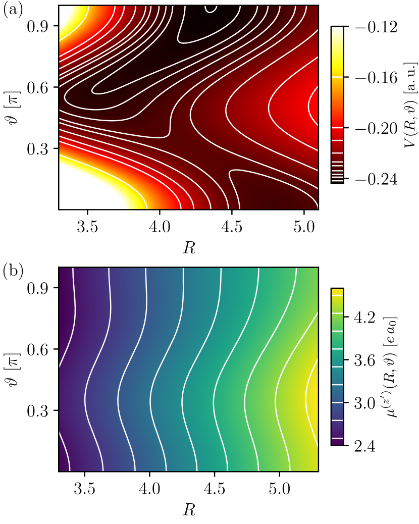
Figure 2: (a) The potential energy surface $V(R,\vartheta)$ in Eq. (2) for the LiCN isomerization reaction taken from Ref. Essers et al., 1982. The two stable conformations of LiCN at $\vartheta=0$ and LiNC at $\vartheta=\pi$ are separated by a rank-1 saddle. (b) The $\mu^{(z^{\prime})}(R,\vartheta)$ part of the dipole surface according to Eq. (6). The corresponding analytical form is taken from Ref. Brocks et al., 1984.

We use the potential energy surface $V(R,\vartheta)$ of Ref. Essers et al., 1982 for our calculations. As shown in Fig. 2 (a), there exist two local minima on the energy surface corresponding to the linear structures LiCN ($\vartheta=0$) and LiNC ($\vartheta=\pi$). In between these two minima, at $\vartheta=0.292\,\pi$, a rank-1 saddle represents the bottleneck of the isomerization reaction, visualized by the equipotential lines in Fig. 2 (a). At the energies above the barrier typical for reaction, the motion of the Li atom between the isomers appears as orbits around the cyanide.

The corresponding classical rotationless two degrees of freedom Hamiltonian, as applied to the LiCN reaction,Benito et al. (1989); Vergel et al. (2014) is

$$\mathcal{H}=\frac{p_{R}^{2}}{2\mu_{1}}+\frac{1}{2}\quantity(\frac{1}{\mu_{1}R^{2}}+\frac{1}{\mu_{2}r_{\mathrm{e}}^{2}})p_{\vartheta}^{2}+V(R,\vartheta)\,\text{,}$$ (2)

under the assumption that the canonical momentum $p_{\alpha}=0$ is fixed for non-rotating molecules. Using Hamilton’s formalism, the dynamics of the LiCN $\rightleftharpoons$ LiNC isomerization reaction in the absence of external fields can be obtained for the state $\boldsymbol{\gamma}(t)=\left(\vartheta,p_{\vartheta},R,p_{R}\right)^{\mathrm{T}}$ by numerically integrating a set of first order differential equations for $\dot{\boldsymbol{\gamma}}(t)$, i. e.

$$\dot{\vartheta} =\quantity(\frac{1}{\mu_{1}R^{2}}+\frac{1}{\mu_{2}r_{\mathrm{e}}^{2}})p_{\vartheta}\,\text{,}$$ (3a)

$$\dot{p}_{\vartheta} =-\derivative{V(R,\vartheta)}{\vartheta}\,\text{,}$$ (3b)

$$\dot{R} =\frac{p_{R}}{\mu_{1}}\,\text{,}$$ (3c)

$$\dot{p}_{R} =\frac{p_{\vartheta}^{2}}{\mu_{1}R^{3}}-\derivative{V(R,\vartheta)}{R}\,\text{.}$$ (3d)

In the present work, we adopt a fourth order Runge–Kutta algorithm with a fixed step size.Press et al. (1987) The first derivatives of the potential in Eqs. (3) have been implemented analytically in C++.

II.1.2 Driven isomerization reaction

The aim of this work is to reveal how external driving influences the decay rates of the reactant population close to the TS. Such external driving can be induced by a time-dependent homogeneous electric field along a fixed direction. We call this the $z$ direction, and write the driving term as

$$\boldsymbol{E}(t)=E_{0}\sin(\omega t)\hat{\mathbf{e}}_{z}\,\text{,}$$ (4)

which couples to the molecule’s dipole moment $\boldsymbol{\mu}$. This makes the Hamiltonian of Eq. (3) time-dependent through the added term

$$V_{\mathrm{dip}}(t)=-\boldsymbol{\mu}\dotproduct\boldsymbol{E}(t)$$ (5)

to the potential energy.Jackson (2012) To complete the equations, however, we must now also specify a continuous representation for the molecule’s dipole moment $\boldsymbol{\mu}$, the so-called dipole surface, accounting for the fact that the underlying electronic wave functions vary as a function of the Born-Oppenheimer coordinates.

Individual points of the dipole surface have earlier been obtained using SCF methods.Essers et al. (1982) Motivated by the success of Wormer and co-workersWormer and Tennyson (1981); Essers et al. (1982) in representing the SCF potential energy surface, Brocks et al.Brocks et al. (1984) constructed analytical expressions $(\mu^{(x^{\prime})}(R,\vartheta),\mu^{(z^{\prime})}(R,\vartheta))$ for the dipole moment of LiCN in the body-fixed reference frame (see Fig. 1). We use this dipole surface with the corrections involving sign errors, noted recently by Borondo and coworkers.Murgida et al. (2015) The $z^{\prime}$-part of this dipole surface, which is at least $15$ times larger than the dipole moment $\mu^{(x^{\prime})}$ in the $x^{\prime}$-direction, is shown in Fig. 2 (b). The body-fixed and space-fixed coordinate systems differ by a rotation with angle $\alpha$, and thus the dipole moment in the space-fixed coordinate system reads

$$\boldsymbol{\mu}(R,\vartheta,\alpha)=\matrixquantity(\cos\alpha&\sin\alpha\\ -\sin\alpha&\cos\alpha)\matrixquantity(\mu^{(x^{\prime})}(R,\vartheta)\\ \mu^{(z^{\prime})}(R,\vartheta))\,\text{.}$$ (6)

Neglecting the small component $\mu^{(x^{\prime})}(R,\vartheta)$ in Eq. (5) the dipole potential now reads

$$V_{\mathrm{dip}}(R,\vartheta,\alpha,t)\approx-E_{0}\sin(\omega t)\mu^{(z^{\prime})}(R,\vartheta)\cos\alpha\,\text{.}$$ (7)

We then further approximate $\cos\alpha\approx 1$ removing the corrections from the oscillations in $\alpha$ around the minimum at $\alpha=0$, and allowing us to reduce the dimensionality to only the two remaining degrees of freedom, $R$ and $\vartheta$. Although we have not fully explored the most general conditions for which this approximation will be valid, at the very least they will be satisfied when the oscillations in $\alpha$ are faster than the other motion. In this limit, the potential on $(R,\vartheta)$ results from the effective field obtained from the average over $\alpha$, and reduces to a form with a renormalized prefactor, $E_{0}$, and no $\alpha$ dependence. We can thus focus on the reduced-dimensional Hamiltonian

$$\mathcal{H}_{\mathrm{driven}}(R,\vartheta,t)=\mathcal{H}+V_{\mathrm{dip}}(R,\vartheta,t)\,\text{,}$$ (8)

where $\mathcal{H}$ is the non-driven Hamiltonian of Eq. (2) and the time-dependent driving is included via the dipole potential

$$V_{\mathrm{dip}}(R,\vartheta,t)=-E_{0}\mu^{(z^{\prime})}(R,\vartheta)\sin(\omega t)\,\text{.}$$ (9)

The equations of motion take the same form as for the non-driven case given in Eqs. (3) with $V$ replaced by the (time-dependent) potential

$$V_{\mathrm{driven}}(R,\vartheta,t)=V(R,\vartheta)+V_{\mathrm{dip}}(R,\vartheta,t)\,\text{.}$$ (10)

Again, solutions are found numerically using a fourth order Runge–Kutta algorithmPress et al. (1987) and a C++ implementation of the derivatives of $V_{\mathrm{driven}}$ with respect to $R$ and $\vartheta$.

III Results and discussion

The relative movement of individual atoms in the non-driven LiCN $\rightleftharpoons$ LiNC isomerization reaction is described by trajectories obtained via the propagation of an initial state according to Eq. (3). The evolving state is identifiable as reactant $\mathcal{R}$ if $\vartheta<0.15\,\pi$ and product $\mathcal{P}$ if $\vartheta>0.5\,\pi$ when it is found in the corresponding regions highlighted in Fig. 3 (a). The contours of the potential are also shown, providing a view of the underlying channel for trajectories to go between $\mathcal{R}$ and $\mathcal{P}$.

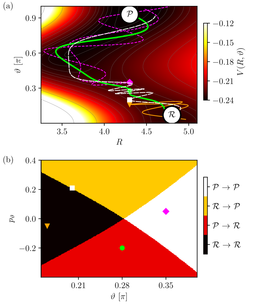
Figure 3: Reactive and non-reactive behavior of trajectories initially launched close to the barrier region (illustrated with individual markers), and propagated according to Eqs. (3) forward and backward in time until the reactant $\mathcal{R}$ or product $\mathcal{P}$ state is reached. (a) $(R,\vartheta)$ position space representation with the potential energy surface according to Fig. 2 (a) as shown in color (or shading in print) defined by the bar to its right. (b) $(\vartheta,p_{\vartheta})$ cross-section of the phase space with the reactive and non-reactive regions encoded in color (or shading in print) defined by the bar to its right. For all trajectories, the remaining coordinate $p_{R}$ is initially set to zero.

In Fig. 3 (a), representative trajectories are initialized at $(R=4.3,p_{R}=0)$ for four different combinations of $\vartheta$ and $p_{\vartheta}$ as also highlighted by the corresponding marker in Fig. 3 (b). Each full trajectory, displayed with a different line style, is obtained by propagating the initial point in phase space according to Eqs. (3) forward and backward in time until the reactant or the product state is reached. Two of these trajectories are reactive (thick solid green with initial circle, thin dashed white with initial square) and the other two (thin solid yellow with initial triangle, thin dashed purple with initial diamond) are not since their energy is too low to cross the barrier.

The shaded regions of Fig. 3 (b) label the reactive ($\mathcal{R}\to\mathcal{P}$ and $\mathcal{P}\to\mathcal{R}$) and non-reactive ($\mathcal{R}\to\mathcal{R}$ and $\mathcal{P}\to\mathcal{P}$) initial points in the $(\vartheta,p_{\vartheta})$ subspace. These regions are separated by the stable and the unstable manifolds which intersect at a particular point $(\vartheta,p_{\vartheta})^{\mathrm{NHIM}}$ of the NHIM for $(R=4.3,p_{R}=0)$. The white dashed square trajectory is initialized closest to one of the manifolds and stays in the barrier region for nearly three oscillations in the stable direction of the barrier. Hence, it crosses a corresponding DS separating reactants from products closest to the NHIM. While the structures illustrated in Fig. 3 were previously seen in a generic model system with a driven rank-1 saddle,Feldmaier et al. (2017); Bardakcioglu et al. (2018); Feldmaier et al. (2019a, b) the results here show that they are realized also in a specific model of a chemical reaction. In both cases, the geometry is described by the stable and unstable manifolds of the barrier, and the nature of the reactivity is determined by the associated DS attached to the NHIM.

III.1 Dynamics of periodically driven transition states

When periodically driving the LiCN $\rightleftharpoons$ LiNC isomerization reaction, the potential $V_{\mathrm{dip}}(R,\vartheta,t)$ in Eq. (9) is explicitly time-dependent and the energy of the system is no longer conserved. Still, a two-dimensional NHIM exists in the barrier region, which contains all trajectories that never leave this region, neither forward, nor backward in time. In contrast to a static system, however, the NHIM becomes time-dependent. For periodic driving, such a NHIM oscillates with the same frequency as that of the driving of the barrier because of the symmetry of the system with respect to time.

The Poincaré surface of section (PSOS) is a useful tool for resolving the dynamics of this time-dependent NHIM in a periodically driven system. Therein, the positions $(R,p_{R})$ of several trajectories on the NHIM are marked after integer multiples of the driving period for a time much longer than a single period of the external driving. When propagating trajectories for such a relatively long time, the instability of the dynamics in the NHIM can become problematic as errors produced by any numerical propagator are exponentially increasing. Consequently, trajectories initialized as precisely as possible in the NHIM nevertheless “fall down” from the barrier to either the reactant or the product side. This problem can be addressed through the use of a stabilized propagator,Tschöpe et al. (2020); Feldmaier et al. (2019b) which successively projects unstable trajectories back into the NHIM after an appropriately chosen time step using the binary contraction method (BCM).

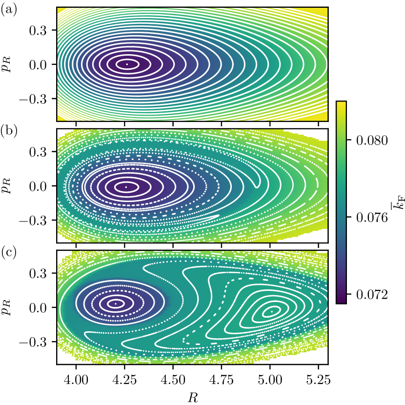
Figure 4: The stable structures obtained from the dynamics on the NHIM are compared to Floquet rates $\overline{k}_{\mathrm{F}}$ for the decay of trajectories from the NHIM for the static (a) and the driven LiCN isomerization reaction with $E_{0}=0.01$ and $\omega=0.01\,\pi$ in (b) and $\omega=0.02\,\pi$ in (c), respectively. The white curves in all three panels are the PSOSs obtained from periodic orbits in (a), and from the propagation of trajectories for $400$ periods of the external driving while marking their instantaneous position $(R,p_{R})$ after each period in (b) and (c). The color encoding shows the mean Floquet rates obtained for $100\times 100$ stabilized trajectories which are initialized on an equidistant grid for the ranges of $R\in[3.8,5.3]$ and $p_{R}\in[-0.5,0.5]$ on the NHIM. Its contours (not shown but indicated through the color variation) coincide with the PSOS. All trajectories are stabilized to the NHIM using the BCM with a tolerance of $10^{-12}$ and the colors are interpolated using bicubic splines.

In the static case according to Eq. (2), the energy is conserved, so each trajectory in Fig. 4 (a) is periodic. The central fixed point corresponds to the trajectory resting at the saddle point of the barrier—viz. at $R=4.2626$ and $\vartheta=0.2800\,\pi$. The frequency of oscillations in the stable direction of the static barrier decreases monotonously from about $\omega_{\mathrm{orth}}=0.043\,\pi$ for the trajectories close to the fixed point to, e. g., about $\omega_{\mathrm{orth}}=0.035\,\pi$ for a trajectory with energy $E=-0.19$. The driving frequencies, chosen below, range between 2 to 4 times slower than the oscillation frequencies of the orthogonal modes and thus provide a non-trivial perturbation to the system. The PSOSs at these driving frequencies indeed show significant changes compared to the static case as shown in Fig. 4.

For the driven systems, the stabilized trajectories are initiated on the NHIM at $t_{0}=0$. They are propagated for $400$ periods of the external driving with amplitude $E_{0}=0.01$ and frequency $\omega=0.01\,\pi$. Specifically, the values are chosen to correspond to an electromagnetic field with frequency $4.85\text{\,}\mathrm{THz}$ (wavelength $\lambda=$61.9\text{\,}\mathrm{\SIUnitSymbolMicro m}$$) and amplitude $E_{0}=$5.14\text{\times}{10}^{7}\text{\,}\mathrm{V}\text{\,}{\mathrm{cm}}^{-1}$$. After each period of $T=200$, the instantaneous position $(R,p_{R})$ of each trajectory in the NHIM is marked. The stabilization of each trajectory into the NHIM was performed using the BCM with an error tolerance of $10^{-12}$. Finally, we observe that the PSOSs for the driving cases look quite different from the static case because the driven NHIM is time-dependent.

The driven trajectories are generally no longer periodic and energy is not conserved, leading to a more complex geometric structure. Nevertheless, at first glance, the structure of the trajectories of the driven barrier in Fig. 4 (b) looks very similar to those of the non-driven barrier in Fig. 4 (a) having a central fixed point and tori (trajectories in the non-driven case) around it. On the right-hand side of Fig. 4 (b) at about $R=4.8$ and $p_{R}=-0.2$, an unstable fixed point is visible, interruption the regular arrangement of the tori. According to the Poincaré-Birkhoff theorem,Wimberger (2014) only an even number of fixed points may occur in a perturbed system (if regarded not precisely at the bifurcation values), and consequently, the appearance of the unstable fixed point is accompanied by the emergence of a stable fixed point. The latter is located approximately at $R=3.9$ and $p_{R}=0$ and is not directly visible here.

To magnify the influence of the moving barrier, the PSOS in Fig. 4 (c) is obtained in the same way as in Fig. 4 (b) but with twice the frequency of the external driving $\omega=0.02\,\pi$. Physically, this corresponds to an electromagnetic field with frequency $9.70\text{\,}\mathrm{THz}$ (wavelength $\lambda=$30.9\text{\,}\mathrm{\SIUnitSymbolMicro m}$$).Note (2) Now, the external driving has a strong impact on the dynamics of the trajectories on the NHIM. An additional unstable and an additional stable fixed point are clearly visible. Both stable fixed points belong to separate period-1 trajectories, that are encircled by many quasi-periodic trajectories on various tori. These structures, not seen in the non-driven barrier and only partially seen with weak driving, arise solely due to the external driving.

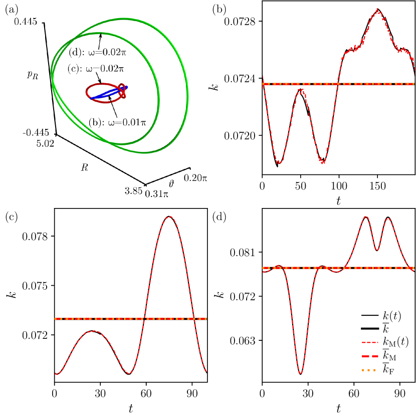
Figure 5: (a) Representation $(R,\vartheta,p_{R})$ of period-1 trajectories on the NHIM of the driven LiCN isomerization reaction. The inner trajectory corresponds to the central elliptic fixed point in Fig. 4 (b), the intermediate and outer double-loop trajectories to the elliptic fixed points in Figs. 4 (c) and 4 (d) at positions $R\approx 4.2$ and $R\approx 5.0$, respectively. Parts (b)-(d) show the instantaneous ensemble rate $k(t)$ (thin black line), the time-averaged mean ensemble rate $\overline{k}$ (thick black horizontal line), the mean Floquet rate $\overline{k}_{\mathrm{F}}$ (orange dotted horizontal line), the instantaneous manifold rate $k_{\mathrm{M}}(t)$ (thin red dashed line), and the time-averaged mean manifold rate $\overline{k}_{\mathrm{M}}$ (thick red horizontal dashed line). The methods for obtaining these various rates are described in the supplementary material.

A three-dimensional representation $(R,\vartheta,p_{R})$ of the three periodic trajectories corresponding to the stable fixed points clearly shown in Fig. 4 (b) and (c) is given in Fig. 5 (a). Here, the inner trajectory, corresponding to the visible stable fixed point in Fig. 4 (b) at initial position $R=4.2579$ and $p_{R}=-0.0117$ shows just very little movement in the stable direction of the barrier. However, the trajectory in between, corresponding to the stable fixed point at $R=4.2040$ and $p_{R}=0.0313$ and especially the outer trajectory, corresponding to the stable fixed point at $R=5.0096$ and $p_{R}=-0.0378$ of Fig. 4 (c) are subject to significant movement in the stable direction of the barrier. Note, that these two trajectories show two oscillations in direction of the orthogonal mode of the barrier although they are both period-1 trajectories with respect to the external driving.

III.2 Instantaneous decay near periodic trajectories on the driven NHIM

Using the methods introduced in Ref. Feldmaier et al., 2019b and discussed as supplementary material, the instantaneous reactant decay rates associated with trajectories on the driven NHIM can be obtained. First, we analyze the three period-1 trajectories displayed in Fig. 5 (a). The inner trajectory—shown in blue (in color) on the (a) panel—is obtained for a driving frequency of $\omega=0.01\,\pi$, while the two outer trajectories—shown in blue and green (in color) on the (a) panel—are obtained for a system with a larger driving frequency of $\omega=0.02\,\pi$, as labeled.

Figure 5 (b) presents the instantaneous decay rates associated with trajectories close to the inner period-1 trajectory with an initial point $R=4.2579$ and $p_{R}=-0.0117$ at time $t=0$ on the NHIM of a driven barrier with $E_{0}=0.01$ and $\omega=0.01\,\pi$. To obtain decay rates with the ensemble method, the trajectory is divided into $20$ segments. For each segment, an ensemble of $200$ reactive trajectories is initialized close to the NHIM with a distance of $\Delta\vartheta=10^{-3}$. Patching together these individual segments yields the thin black line in Fig. 5 (b). The corresponding mean ensemble decay rate is obtained by averaging over a full period of the external driving, yielding $\overline{k}=0.0724$ and displayed as a thick solid vertical line. This result can be verified using the Floquet method, see supplementary material, which yields a mean Floquet rate of $\overline{k}_{\mathrm{F}}=0.0724$ for this trajectory. This mean Floquet rate, shown as an orange dotted vertical line in Fig. 5 (b), is in perfect agreement with the mean ensemble rate. Using the local manifold analysis (LMA), see supplementary material, a third verification of these decay rates can be obtained. The thin red dashed line in Fig. 5 (b) marks the instantaneous manifold rate $k_{\mathrm{M}}(t)$ and the thick red dashed vertical line marks the mean manifold rate $\overline{k}_{\mathrm{M}}=0.0724$, averaged over a full period of the external driving. Both lines fit the results of the other two methods.

The same procedure used to obtain Fig. 5 (b) is repeated for the two remaining trajectories of Fig. 5 (a). Figures 5 (c) and 5 (d) present the results for the intermediate trajectory (labeled c, and red in color), and the outer trajectory (labeled d, and green in color) in Fig. 5 (a), respectively. In both cases, the instantaneous decay rates obtained via the LMA correspond perfectly to the instantaneous decay rates of the ensemble method, and their mean rates are also in perfect agreement with the obtained Floquet rates. Hence, $\overline{k}=\overline{k}_{\mathrm{M}}=\overline{k}_{\mathrm{F}}=0.0730$ for the intermediate trajectory, and $\overline{k}=\overline{k}_{\mathrm{M}}=\overline{k}_{\mathrm{F}}=0.0778$ for the outer trajectory.

The decay of the reactant population close to the three different period-1 trajectories in Figs. 5 (b)-(d) is represented by very different instantaneous rates, and consequently also mean rates. In addition, the amount of variation of the instantaneous rates varies strongly for each trajectory. For the inner trajectory that according to Fig. 5 (a) has the smallest movement in the orthogonal mode, the relative change of the instantaneous rate, $\Delta k\approx 10^{-3}$, is very small. Consequently, the effect of the external driving is barely noticeable. The intermediate trajectory of Fig. 5 (a) has significantly more motion in the stable direction of the barrier. The relative change, $\Delta k\approx 10^{-2}$, of the instantaneous rate is considerably larger as seen in Fig. 5 (c). The outer trajectory of Fig. 5 (a) has by far the largest movement in the stable direction of the barrier. The relative change, $\Delta k\approx 0.5\times 10^{-1}$, in the instantaneous rates in Fig. 5 (d) is also the largest. Thus, we can conclude that the influence of the external driving is high if a trajectory has significant motion in the direction of the orthogonal modes. Further evidence for this effect follows in Sec. III.3 in the context of the decay rates associated with the numerous quasi-periodic trajectories on the driven NHIM.

III.3 Phase-space resolved decay rates

We now obtain the phase-space resolved decay rates of the reactant population close to arbitrary trajectories on the NHIM of the periodically driven LiCN $\rightleftharpoons$ LiNC isomerization reaction. As seen above, all three methods to calculate the decay of reactant population close to the TS result in the same values for a specific period-1 trajectory, and hence we choose only one of these for the present calculation. Namely, the Floquet method is employed because it is relatively easy to implement and computationally fast to evaluate.

In all the cases of Fig. 4, the Floquet rates are overlayed on top of the PSOSs. They are obtained on equidistant grids using approximately $10\,000$ stabilized trajectories, and they are displayed through a shaded (or colored in color) encoding. All trajectories are propagated for a total time up to $t=$10\,000$$ as needed to converge. The individual Floquet rates are interpolated using bicubic splines to smooth the discrete points. We found that the decay rates of all the trajectories located on the corresponding regular tori are indeed the same. This is expected since any quasi-periodic trajectory on such a torus in general covers it in full if propagated for long enough. Thus, a unique decay rate is associated with each torus. This observation is true for the static system using a simpler argument. Namely, the Floquet rate reduces to a property of any of the periodic trajectories on the static NHIM because the tori is necessarily periodic.

When comparing the obtained mean Floquet rates of the driven system with $E_{0}=0.01$ and $\omega=0.01\,\pi$ in Fig. 4 (b) to the mean Floquet rates of the static system according to Fig. 4 (a), the influence of the external driving is small. In Fig. 4 (b), the mean Floquet rate obtained at the clearly visible elliptic fixed point in the center of the tori corresponds to the rates already obtained in Fig. 5 (b) with all three methods introduced in Ref. Feldmaier et al., 2019b and provided as supplementary material. In the two cases of Fig. 4 (a) and Fig. 4 (b), the mean Floquet rates at the central fixed point are similar—that is, they are $\overline{k}_{\mathrm{F}}=0.0721$ and $\overline{k}_{\mathrm{F}}=0.0724$, respectively. The primary difference is the emergence of structure that is barely visible here but more clearly visible in Fig. 4 (c) as discussed below.

A further increase in the frequency of the external driving to $\omega=0.02\,\pi$ leads to a drastic change in the structure as shown in Fig. 4 (c). Two clearly separated elliptical fixed points are now visible in the PSOS with each encircled by an individual set of tori dividing the NHIM into two regions of very different Floquet rates. This means that two regions of very different stability emerge on the periodically driven NHIM. In the surrounding of the fixed point at $R=4.2040$ and $p_{R}=0.0313$, the decay rates of the reactant population are rather small and approximately correspond to the mean Floquet rate of $\overline{k}_{\mathrm{F}}=0.0730$ obtained for the central period-1 trajectory according to Fig. 5 (c). On the other hand, the mean Floquet rates in a region near the fixed point at $R=5.0096$ and $p_{R}=-0.0378$ are rather large and approximately correspond to the mean Floquet rate $\overline{k}_{\mathrm{F}}=0.0778$ of the associated central period-1 trajectory according to Fig. 5 (d).

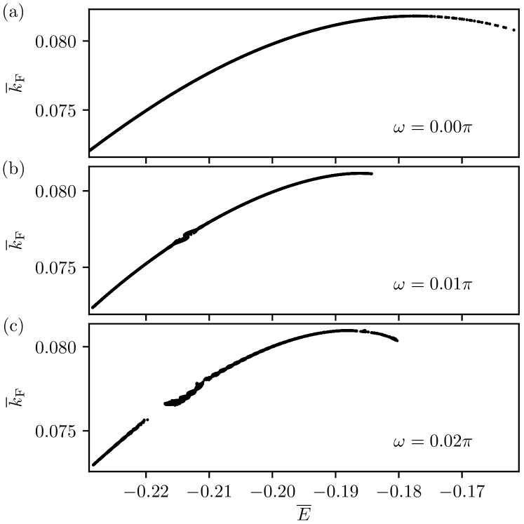
Figure 6: The quantitative relation of the Floquet rates $\overline{k}_{\mathrm{F}}$ to the mean energies $\overline{E}$ of trajectories on the NHIM obtained at three different driving frequencies $\omega$ equal to $0.00\,\pi$, $0.01\,\pi$ and $0.02\,\pi$ are shown in panels (a), (b) and (c), respectively. Each rate corresponds to a torus in Fig. 4 at the mean energy $\overline{E}$.

For a periodically driven system, the instantaneous energy $E(t)$ of trajectories in the NHIM is not conserved. However, by averaging the instantaneous and non-conserved energy of a given trajectory over many oscillations of the periodic driving, the mean energy $\overline{E}$ of a specific torus is well defined and characteristic of the trajectory and its associated initial condition. The quantitative correspondence between the mean energy of a trajectory and the Floquet rate is revealed in Fig. 6 by plotting the Floquet rates obtained in Fig. 4 with respect to the corresponding (mean) energies of the trajectories.

As a control for the driven cases, Fig. 6 (a) shows the relation between the Floquet rate and the mean energy for the non-driven system of Fig. 4 (a). In this limit, energy is conserved. Thus the mean energy $\overline{E}$ corresponds to the instantaneous energy $E(t)$ of the respective trajectories. According to Fig. 6 (a), the relation between the energy and the Floquet rate in the static case is not monotonic and has a maximum at approximately $E=-0.18$. A further increase of the energy of trajectories on the NHIM goes together with a decrease in the corresponding decay rate of the reactant population close to the TS. However, a maximum in these decay rates is associated with a minimum in the stability of the activated complex close to the TS. According to Fig. 6 (a), there seems to be a lower bound for the stability of this activated complex in the non-driven LiCN isomerization reaction.

The results for the driven system in Figs. 6 (b) for $\omega=0.01\,\pi$ and in Fig. 6 (c) for $\omega=0.02\,\pi$ correspond to cases in Fig. 4 (b) and (c), respectively. Despite the driving, they retain some similarity with the static case of Fig. 6 (a). Again, the relation between the Floquet rate of a trajectory on a given torus and the associated mean energy is non-monotonic and there seems to exist a maximum decay rate for the reactant population associated with trajectories on the NHIM.

In contrast to the static case, however, for the driven barrier case with $\omega=0.02\,\pi$, a significant gap arises in the curve of Fig. 6 (c) at about $\overline{E}=-0.22$. This gap corresponds exactly to the emergence of tori around distinct fixed points seen in Fig. 4 (c). At the beginning of the upper edge of the gap in Fig. 6 (c), the curve initially fluctuates before becoming smooth again with increasing mean energy. The origin of this behavior is numerical because the Floquet method for non-periodic trajectories is defined only in the limit $t\to\infty$ (see supplementary material). However, trajectories in Fig. 4 (c) are necessarily propagated for a finite time, and this leads to errors in the calculated Floquet rates which are small and appear as fluctuations. In other words, close to the boundary between the two regions of the different decay rates on the driven NHIM, the circulation times of quasi-periodic trajectories on the regular tori increases and longer propagation times are necessary to obtain a desired accuracy using the Floquet method. This behavior can also be seen in Fig. 6 (b) for the case with a driving frequency of $\omega=0.01\,\pi$. A second stable fixed point is barely visible in Fig. 4 (b). Consequently, nearly no gap appears in Fig. 6 (b). Nevertheless, fluctuations are visible at the energy of the indicated fixed point on the left-hand side of Fig. 4 (b), and, hence, a gap is just emerging there.

IV Conclusion and Outlook

In this paper, we study the influence of a periodically oscillating external field on the LiCN $\rightleftharpoons$ LiNC isomerization reaction. In the static case, the energy is conserved and all trajectories on the associated NHIM are periodic. For a periodically driven system, nearly all trajectories contained in the NHIM are quasi-periodic and located on stable tori. The dynamics on the driven NHIM has been revealed by means of a PSOS. Depending on the frequency of the external field, a new set of tori around a second stable fixed point emerges on the NHIM.

The associated mean decay rates of reactant population in a close neighborhood of the periodic or quasi-periodic trajectories on the NHIM are obtained by various methods.Feldmaier et al. (2019b) Both in the static and driven cases, the decay rates differ significantly across these neighborhoods, and are approximately prescribed by the mean decay rates associated to the corresponding central periodic trajectory. The instantaneous decay rates for these central trajectories are also sensitive to the driving. Specifically, the relation between the mean decay rates associated with a specific torus and the corresponding mean energy of trajectories on this torus is non-trivial. There are two clearly distinguished regions associated with different mean decay rates of the reactant population close to the TS. They are approximately prescribed by period-1 trajectories identified at the center of the corresponding tori of the PSOS. They are consequently not continuously connected and a significant gap between the corresponding decay rate emerges. The regularity of the structure of the PSOS for the trajectories near the NHIM is not chaotic as one might have expected given the recently observed chaotic sea in the global phase space.Revuelta et al. (2019) This points to the simplification arising from considering decay rates in the local neighborhood of the TS. Future work to extend these decay rates to the global rates thus needs to consider not just the possibility of additional barrier regions but also the complex dynamics that can arise from chaotic regions.

Thus the influence of the periodic external driving on the LiCN $\rightleftharpoons$ LiNC isomerization reaction is large when compared to the static problem. Indeed, the emergence of different regions of the reactant population decay for the driven LiCN $\rightleftharpoons$ LiNC isomerization reaction as well as the existence of gaps in both energy and decay rate between these separate regions are effects solely invoked by the external driving.

The possible effects from our approximate simplification of the LiCN $\rightleftharpoons$ LiNC isomerization reaction to a body-fixed axes may need to be addressed. This would allow the molecules to rotate with respect to the external field and increase the dimensionality of the coordinate space of the problem beyond the two-dimensional case considered here. However, there is precedent from the earlier work of Ref. Murgida et al., 2015 that the reaction is much faster than the rotation and hence such effects are small. One could also include a Langevin-type description of the dynamics—according to, e. g., Ref. Junginger et al., 2016—to address the effects on the decay rates from a solvent as represented by the inclusion of both noise and friction. Alternatively, the effects on the decay rates from an all-atom solvent can be uncovered by inferring the stability of the NHIM from molecular dynamics trajectories. For example, the position of reactive trajectories across the DS can be tracked simulations of LiCN in an argon bath such as those of Refs. García-Müller et al., 2008, 2012, 2014; Junginger et al., 2016. Applying an appropriate external driving could shift these reaction positions to different regions of the NHIM and increases the reaction rate. From the results of the current work, we would expect that there would once again emerge different regions in the PSOS and the corresponding reactant decay rates which should be interpretable as reactive channels. When applying an appropriate external field a second and faster reactive channel with higher decay rates opens up and might serve to an increase of the reaction rate.

Supplementary material

In the supplementary material, we provide a detailed description of the methods used in the primary text. We summarize the details for the implementation of three approaches in determining the decay rates: Floquet analysis, ensemble method, and the local manifold analysis. We also present a technical derivation of the last of these methods.

Data Availability

The data that support the findings of this study are available from the corresponding author upon reasonable request.

References

References

- Eyring (1935) H. Eyring, J. Chem. Phys. 3, 107 (1935), doi:10.1063/1.1749604.
- Wigner (1937) E. P. Wigner, J. Chem. Phys. 5, 720 (1937), doi:10.1063/1.1750107.
- Pollak et al. (1980) E. Pollak, M. S. Child, and P. Pechukas, J. Chem. Phys. 72, 1669 (1980), doi:10.1063/1.439276.
- Pechukas (1981) P. Pechukas, Annu. Rev. Phys. Chem. 32, 159 (1981), doi:10.1146/annurev.pc.32.100181.001111.
- Truhlar et al. (1996) D. G. Truhlar, B. C. Garrett, and S. J. Klippenstein, J. Phys. Chem. 100, 12771 (1996), doi:10.1021/jp953748q.
- Carpenter (2005) B. K. Carpenter, “Potential energy surfaces and reaction dynamics,” in Reactive Intermediate Chemistry (John Wiley & Sons, Ltd, 2005) Chap. 21, pp. 925–960.
- Mullen et al. (2014) R. G. Mullen, J.-E. Shea, and B. Peters, J. Chem. Phys. 140, 041104 (2014), doi:10.1063/1.4862504.
- Arrhenius (1889) S. Arrhenius, Z. Phys. Chem. (Leipzig) 4, 226 (1889), translated and published in Margaret H. Back and Keith J. Laidler, eds., Selected Readings in Chemical Kinetics (Oxford: Pergamon, 1967).
- Laidler (1984) K. J. Laidler, J. Chem. Educ. 61, 494 (1984), doi:10.1021/ed061p494.
- Pollak (1990) E. Pollak, J. Chem. Phys. 93, 1116 (1990), doi:10.1063/1.459175.
- Pollak (1996) E. Pollak, in Dynamics of Molecules and Chemical Reactions, edited by R. E. Wyatt and J. Zhang (Marcel Dekker, New York, 1996) pp. 617–669.
- Uzer et al. (2002) T. Uzer, C. Jaffé, J. Palacián, P. Yanguas, and S. Wiggins, Nonlinearity 15, 957 (2002), doi:10.1088/0951-7715/15/4/301.
- Komatsuzaki and Berry (2001) T. Komatsuzaki and R. S. Berry, Proc. Natl. Acad. Sci. U.S.A. 98, 7666 (2001), doi:10.1073/pnas.131627698.
- Komatsuzaki and Berry (2002) T. Komatsuzaki and R. S. Berry, Adv. Chem. Phys. 123, 79 (2002), doi:10.1002/0471231509.ch2.
- Bartsch et al. (2005a) T. Bartsch, R. Hernandez, and T. Uzer, Phys. Rev. Lett. 95, 058301 (2005a), doi:10.1103/PhysRevLett.95.058301.
- Pollak and Talkner (2005) E. Pollak and P. Talkner, Chaos 15, 026116 (2005), doi:10.1063/1.1858782.
- Bartsch et al. (2008) T. Bartsch, J. M. Moix, R. Hernandez, S. Kawai, and T. Uzer, Adv. Chem. Phys. 140, 191 (2008), doi:10.1002/9780470371572.ch4.
- Hernandez et al. (2010) R. Hernandez, T. Bartsch, and T. Uzer, Chem. Phys. 370, 270 (2010), doi:10.1016/j.chemphys.2010.01.016.
- Waalkens et al. (2008) H. Waalkens, R. Schubert, and S. Wiggins, Nonlinearity 21, R1 (2008), doi:10.1088/0951-7715/21/1/R01.
- Wiggins (2016) S. Wiggins, Regul. Chaotic Dyn. 21, 621 (2016), doi:10.1134/S1560354716060034.
- Ezra et al. (2009) G. S. Ezra, H. Waalkens, and S. Wiggins, J. Chem. Phys. 130, 164118 (2009), doi:10.1063/1.3119365.
- Fenichel (1972) N. Fenichel, Indiana Univ. Math. J. 21, 193 (1972), doi:10.1512/iumj.1972.21.21017.
- Wiggins (1994) S. Wiggins, Normally Hyperbolic Invariant Manifolds in Dynamical Systems (Springer, New York, 1994).
- Feldmaier et al. (2017) M. Feldmaier, A. Junginger, J. Main, G. Wunner, and R. Hernandez, Chem. Phys. Lett. 687, 194 (2017), doi:10.1016/j.cplett.2017.09.008.
- Feldmaier et al. (2019a) M. Feldmaier, P. Schraft, R. Bardakcioglu, J. Reiff, M. Lober, M. Tschöpe, A. Junginger, J. Main, T. Bartsch, and R. Hernandez, J. Phys. Chem. B 123, 2070 (2019a), doi:10.1021/acs.jpcb.8b10541.
- Pollak and Pechukas (1978) E. Pollak and P. Pechukas, J. Chem. Phys. 69, 1218 (1978), doi:10.1063/1.436658.
- Pechukas and Pollak (1979) P. Pechukas and E. Pollak, J. Chem. Phys. 71, 2062 (1979), doi:10.1063/1.438575.
- Hernandez and Miller (1993) R. Hernandez and W. H. Miller, Chem. Phys. Lett. 214, 129 (1993), doi:10.1016/0009-2614(93)90071-8.
- Hernandez (1994) R. Hernandez, J. Chem. Phys. 101, 9534 (1994), doi:10.1063/1.467985.
- Wiggins et al. (2001) S. Wiggins, L. Wiesenfeld, C. Jaffe, and T. Uzer, Phys. Rev. Lett. 86 (2001), doi:10.1103/PhysRevLett.86.5478.
- Jaffé et al. (2002) C. Jaffé, S. D. Ross, M. W. Lo, J. Marsden, D. Farrelly, and T. Uzer, Phys. Rev. Lett. 89, 011101 (2002), doi:10.1103/PhysRevLett.89.011101.
- Teramoto et al. (2011) H. Teramoto, M. Toda, and T. Komatsuzaki, Phys. Rev. Lett. 106, 054101 (2011), doi:10.1103/PhysRevLett.106.054101.
- Li et al. (2006) C.-B. Li, A. Shoujiguchi, M. Toda, and T. Komatsuzaki, Phys. Rev. Lett. 97, 028302 (2006), doi:10.1103/PhysRevLett.97.028302.
- Waalkens and Wiggins (2004) H. Waalkens and S. Wiggins, J. Phys. A 37, L435 (2004), doi:10.1088/0305-4470/37/35/L02.
- Çiftçi and Waalkens (2013) U. Çiftçi and H. Waalkens, Phys. Rev. Lett. 110, 233201 (2013), doi:10.1103/PhysRevLett.110.233201.
- Mancho et al. (2003) A. M. Mancho, D. Small, S. Wiggins, and K. Ide, Physica D 182, 188 (2003), doi:10.1016/S0167-2789(03)00152-0.
- Craven and Hernandez (2015) G. T. Craven and R. Hernandez, Phys. Rev. Lett. 115, 148301 (2015), doi:10.1103/PhysRevLett.115.148301.
- Lopesino et al. (2017) C. Lopesino, F. Balibrea-Iniesta, V. J. García-Garrido, S. Wiggins, and A. M. Mancho, Int. J. Bifurc. Chaos 27, 1730001 (2017), doi:10.1142/S0218127417300014.
- Bardakcioglu et al. (2018) R. Bardakcioglu, A. Junginger, M. Feldmaier, J. Main, and R. Hernandez, Phys. Rev. E 98, 032204 (2018), doi:10.1103/PhysRevE.98.032204.
- Schraft et al. (2018) P. Schraft, A. Junginger, M. Feldmaier, R. Bardakcioglu, J. Main, G. Wunner, and R. Hernandez, Phys. Rev. E 97, 042309 (2018), doi:10.1103/PhysRevE.97.042309.
- Tschöpe et al. (2020) M. Tschöpe, M. Feldmaier, J. Main, and R. Hernandez, Phys. Rev. E 101, 022219 (2020), doi:10.1103/PhysRevE.101.022219.
- Revuelta et al. (2017) F. Revuelta, G. T. Craven, T. Bartsch, F. Borondo, R. M. Benito, and R. Hernandez, J. Chem. Phys. 147, 074104 (2017), doi:10.1063/1.4997571.
- Bartsch et al. (2019) T. Bartsch, F. Revuelta, R. M. Benito, and F. Borondo, Phys. Rev. E 99, 052211 (2019), doi:0.1103/PhysRevE.99.052211.
- Feldmaier et al. (2019b) M. Feldmaier, R. Bardakcioglu, J. Reiff, J. Main, and R. Hernandez, J. Chem. Phys. 151, 244108 (2019b), doi:10.1063/1.5127539.
- Craven et al. (2014) G. T. Craven, T. Bartsch, and R. Hernandez, J. Chem. Phys. 141, 041106 (2014), doi:10.1063/1.4891471.
- Bartsch et al. (2005b) T. Bartsch, T. Uzer, and R. Hernandez, J. Chem. Phys. 123, 204102 (2005b), doi:10.1063/1.2109827.
- Truhlar et al. (1982) D. G. Truhlar, A. D. Isaacson, R. T. Skodje, and B. C. Garrett, J. Phys. Chem. 86, 2252 (1982), doi:10.1021/j100209a021.
- Pollak (2000) E. Pollak, in Theoretical Methods in Condensed Phase Chemistry, edited by S. D. Schwartz (Kluwer Academic Publishers, Dordrecht, 2000) pp. 1–46.
- Baraban et al. (2015) J. H. Baraban, P. B. Changala, G. C. Mellau, J. F. Stanton, A. J. Merer, and R. W. Field, Science 350, 1338 (2015), doi:10.1126/science.aac9668.
- Waalkens et al. (2004) H. Waalkens, A. Burbanks, and S. Wiggins, J. Chem. Phys. 121, 6207 (2004).
- McCoy and Sibert III (1991) A. B. McCoy and E. L. Sibert III, J. Chem. Phys. 95, 3476 (1991), doi:10.1063/1.460851.
- Essers et al. (1982) R. Essers, J. Tennyson, and P. E. S. Wormer, Chem. Phys. Lett. 89, 223 (1982), doi:10.1016/0009-2614(82)80046-8.
- Brocks et al. (1984) G. Brocks, J. Tennyson, and A. van der Avoird, J. Chem. Phys. 80, 3223 (1984), doi:10.1063/1.447075.
- García-Müller et al. (2008) P. L. García-Müller, F. Borondo, R. Hernandez, and R. M. Benito, Phys. Rev. Lett. 101, 178302 (2008), doi:10.1103/PhysRevLett.101.178302.
- García-Müller et al. (2012) P. L. García-Müller, R. Hernandez, R. M. Benito, and F. Borondo, J. Chem. Phys. 137, 204301 (2012), doi:10.1063/1.4766257.
- García-Müller et al. (2014) P. L. García-Müller, R. Hernandez, R. M. Benito, and F. Borondo, J. Chem. Phys. 141, 074312 (2014), doi:10.1063/1.4892921.
- Junginger et al. (2016) A. Junginger, P. L. García-Müller, F. Borondo, R. M. Benito, and R. Hernandez, J. Chem. Phys. 144, 024104 (2016), doi:10.1063/1.4939480.
- Vergel et al. (2014) A. Vergel, R. M. Benito, J. C. Losada, and F. Borondo, Phys. Rev. E 89, 022901 (2014), doi:10.1103/PhysRevE.89.022901.
- Prado et al. (2009) S. D. Prado, E. G. Vergini, R. M. Benito, and F. Borondo, Europhys. Lett. 88, 40003 (2009), doi:10.1209/0295-5075/88/40003.
- Murgida et al. (2010) G. E. Murgida, D. A. Wisniacki, P. I. Tamborenea, and F. Borondo, Chem. Phys. Lett. 496, 356 (2010), doi:10.1016/j.cplett.2010.07.057.
- Revuelta et al. (2015) F. Revuelta, R. Chacón, and F. Borondo, Europhys. Lett. 110, 40007 (2015), doi:10.1209/0295-5075/110/40007.
- Murgida et al. (2015) G. E. Murgida, F. J. Arranz, and F. Borondo, J. Chem. Phys. 143, 214305 (2015), doi:10.1063/1.4936424.
- Brocks and Tennyson (1983) G. Brocks and J. Tennyson, J. Mol. Spectrosc. 99, 263 (1983).
- Wormer and Tennyson (1981) P. E. S. Wormer and J. Tennyson, J. Chem. Phys. 75, 1245 (1981), doi:10.1063/1.442174.
- Benito et al. (1989) R. Benito, F. Borondo, J.-H. Kim, B. Sumpter, and G. Ezra, Chem. Phys. Lett. 161, 60 (1989), doi:10.1016/S0009-2614(89)87032-0.
- Press et al. (1987) W. H. Press, S. A. Teukolsky, W. T. Vetterling, and B. P. Flannery, Numerical recipes: The art of scientific computing (Cambridge University Press, New York, 1987).
- Note (1) Throughout the paper, we use atomic units—Bohr radius , elementary charge , and (Hartree)—for length, charge, and energy, but (dalton) as the mass unit. As a consequence, times must be multiplied and frequencies and rates must be divided by a factor of to obtain the corresponding values in atomic units.
- Jackson (2012) J. D. Jackson, Classical electrodynamics (John Wiley & Sons, 2012).
- Note (2) These values have been updated to reflect a correction due to the unit conversion noted in footnote 67.
- Wimberger (2014) S. Wimberger, Nonlinear dynamics and quantum chaos (Springer, Cham, 2014).
- Revuelta et al. (2019) F. Revuelta, R. M. Benito, and F. Borondo, Phys. Rev. E 99, 032221 (2019), doi:10.1103/PhysRevE.99.032221.