A natural extension of Mittag-Leffler function associated with a triple infinite series

Abstract

We establish a new natural extension of Mittag-Leffler function with three variables which is so called ”trivariate Mittag-Leffler function”. The trivariate Mittag-Leffler function can be expressed via complex integral representation by putting to use of the eminent Hankel’s integral. We also investigate Laplace integral relation and convolution result for a univariate version of this function. Moreover, we present fractional derivative of trivariate Mittag-Leffler function in Caputo type and we also discuss Riemann–Liouville type fractional integral and derivative of this function. The link of trivariate Mittag-Leffler function with fractional differential equation systems involving different fractional orders is necessary on certain applications in physics. Thus, we provide an exact analytic solutions of homogeneous and inhomogeneous multi-term fractional differential equations by means of a newly defined trivariate Mittag-Leffler functions.

Keywords: Caputo fractional derivative, special functions, bivariate Mittag-Leffler function, trivariate Mittag-Leffler function, multi-term differential equation

1 Introduction and preliminaries

Special functions are one of the powerful implements in presenting and describing some physical complex phenomena in fractional calculus [1]-[3]. Decades ago, the special function entitled Mittag-Leffler function (M-L) has drawn an arising attention by many researchers due to its importance in solving differential and integral equations with fractional-order in science and engineering [4]-[7].

The classical M–L function which is a natural generalization of the exponential function was proposed by Mittag-Leffler in 1903 as a one-parameter function of one variable by using a single series,

$$E_{\alpha}(s)=\sum_{l=0}^{\infty}\frac{s^{l}}{\Gamma(l\alpha+1)},\quad\alpha\in\mathbb{C},\Re(\alpha)>0,s\in\mathbb{C},$$ (1.1)

and investigated its properties in [8]-[11].

Remark 1.1 ([12]).

The M–L functions are often used in a form where the variable inside the brackets is not $s$ but a fractional power $r^{\alpha}$, or even a constant multiple $\lambda r^{\alpha}$, as follows:

$$E_{\alpha}(\lambda r^{\alpha})=\sum_{l=0}^{\infty}\frac{\lambda^{l}r^{l\alpha}}{\Gamma(l\alpha+1)},\quad\alpha\in\mathbb{C},\Re(\alpha)>0,\lambda,r\in\mathbb{C}.$$

A generalization of (1.1), particularly the two-parameter M–L function was presented by Wiman in 1905 and he determined this function [13, 14] as

$$E_{\alpha,\beta}(s)=\sum_{l=0}^{\infty}\frac{s^{l}}{\Gamma(l\alpha+\beta)},\quad\alpha,\beta\in\mathbb{C},\Re(\alpha)>0,s\in\mathbb{C},$$ (1.2)

which has deeply studied in [15]-[17].

A natural extension of (1.2), which is called the M–L with three-parameter was proposed by Prabhakar [18] in 1971 as

$$E_{\alpha,\beta}^{\delta}(s)=\sum_{l=0}^{\infty}\frac{(\delta)_{l}}{\Gamma(l\alpha+\beta)}\frac{s^{l}}{l!},\quad\alpha,\beta,\delta\in\mathbb{C},\Re(\alpha)>0,s\in\mathbb{C},$$ (1.3)

where $(\delta)_{l}$ is the Pochhammer symbol [19] denoting

$$(\delta)_{l}=\frac{\Gamma(\delta+l)}{\Gamma(\delta)}=\begin{cases*}1,\quad l=0,\delta\neq 0,\\ \delta(\delta+1)\cdots(\delta+l-1),\quad l\in\mathbb{N}.\end{cases*}$$

This series (1.3) is widely used for different applied problems like heat conduction equations with memory [20], electrical circuits [21], Langevin equations [22], anomalous relaxation in dielectrics [23] and fractional order time-delay systems [24, 25, 26]. Note that

$$E_{\alpha,\beta}^{1}(s)=E_{\alpha,\beta}(s),\quad E_{\alpha,1}(s)=E_{\alpha}(s),\quad E_{1}(s)=\exp(s).$$

It is interesting to note that extensions to two or three parameters are well known and thoroughly studied in textbooks [27, 28], but these still involve single power series in one variable. Recently decades, a various type of extensions of M–L functions have been defined: namely ”bivariate” and ”multivariate” M–L functions.

A multi-variable analogue of generalized Mittag-Leffler type function is proposed by Saxena et al. [29] in the form

$$\mathcal{E}^{(\delta_{1},...,\delta_{m})}_{(\rho_{1},...,\rho_{m}),\lambda}(s_{1},...,s_{m})=\sum\limits_{l_{1},...,l_{m}=0}^{\infty}\frac{(\delta_{1})_{l_{1}}...(\delta_{m})_{l_{m}}}{\Gamma(\lambda+\sum\limits_{j=1}^{m}\rho_{j}l_{j})}\frac{s_{1}^{l_{1}}...s_{m}^{l_{m}}}{l_{1}!...l_{m}!},$$ (1.4)

where $\lambda,\rho_{j},\delta_{j},s_{j}\in\mathbb{C},\Re(\rho_{j})>0,j=1,...,m.$

Another multivariable analogue of M–L function $E_{\alpha_{1},...,\alpha_{n}}(s_{1},...,s_{n})$ of $n$ variables $s_{1},...,s_{n}\in\mathbb{C}$ and $n$ parameters $\alpha_{1},...,\alpha_{n},\beta\in\mathbb{C}$ with $\Re(\alpha_{j}),\Re(\beta)>0,j=1,...,n$ is defined by

$$E_{\alpha_{1},...,\alpha_{n}}(s_{1},...,s_{n})=\sum\limits_{k=0}^{\infty}\sum^{l_{1}+...l_{n}=k}_{l_{1}\geq 0,...,l_{n}\geq 0}(k;l_{1},...,l_{n})\frac{\prod\limits_{j=1}^{n}s_{j}^{l_{j}}}{\Gamma(\beta+\sum\limits_{j=1}^{n}\alpha_{j}l_{j})},$$ (1.5)

where

$$(k;l_{1},...,l_{n})\coloneqq\frac{k!}{l_{1}!\times...\times l_{n}!}\quad\text{with}\quad k=\sum_{j=1}^{n}l_{j}.$$

This function (1.5) is studied by Luchko et al. [31] as an analytical solution of the Caputo type fractional differential equations (FDEs) with multi-orders.

It is necessary to point out that various bivariate functions are rising as an extension of the M–L function: one of them is proposed by Özarslan et al. [32] as below:

$$E^{(\rho)}_{\alpha,\beta,q}(u,v)=\sum\limits_{l=0}^{\infty}\sum_{p=0}^{\infty}\frac{(\rho)_{l+p}}{\Gamma(\beta+qp)\Gamma(\alpha+l)}\frac{u^{l}}{l!}\frac{v^{qp}}{p!},$$ (1.6)

under the conditions $\alpha,\beta,q,\rho\in\mathbb{C}\quad\text{with}\quad\Re(\alpha),\Re(\beta)$, and $\Re(q)>0$.

Another a new analogue of classical M–L function which is applied two variables are proposed by Fernandez et al. [33] as follows:

$$E_{\alpha,\beta,\gamma}^{\delta}(u,v)=\sum_{l=0}^{\infty}\sum_{p=0}^{\infty}\frac{(\delta)_{l+p}}{\Gamma(l\alpha+p\beta+\gamma)}\frac{u^{l}v^{p}}{l!p!},\quad\alpha,\beta,\gamma,\delta\in\mathbb{C},\quad\Re(\alpha),\Re(\beta)>0,u,v\in\mathbb{C}.$$ (1.7)

To form a univariate version of (1.7), we write $u=\lambda_{1}r^{\alpha}$ and $v=\lambda_{2}r^{\beta}$ and multiply by a power function:

$$r^{\gamma-1}E_{\alpha,\beta,\gamma}^{\delta}(\lambda_{1}r^{\alpha},\lambda_{2}r^{\beta})=\sum_{l=0}^{\infty}\sum_{p=0}^{\infty}\frac{(\delta)_{l+p}}{\Gamma(l\alpha+p\beta+\gamma)}\frac{\lambda_{1}^{l}\lambda_{2}^{p}}{l!p!}r^{l\alpha+p\beta+\gamma-1}.$$ (1.8)

It is worth noting that the univariate analogue of (1.7) is an exact analytical solution of FDEs system with multi-orders which has been discussed in [34].

Now, we consider another special function which will be introduced later in Section 4. Let $\lambda_{i},\mu_{j}\in\mathbb{C}$, $a_{i},b_{j}\in\mathbb{R}$, for $i=1,2,\ldots,m$, and $j=1,2,\ldots,n$. Generalized Wright function or more appropriately Fox-Wright function $\prescript{}{m}{\Psi_{n}}(\cdot):\mathbb{C}\to\mathbb{C}$ is defined by

$$\prescript{}{m}{\Psi_{n}}(s)=\prescript{}{m}{\Psi_{n}}\left[\begin{array}[]{ccc}(\lambda_{i},a_{i})_{1,m}\\ (\mu_{j},b_{j})_{1,n}\end{array}\Big{|}s\right]=\sum_{l=0}^{\infty}\frac{\prod\limits_{i=1}^{m}\Gamma(\lambda_{i}+a_{i}l)}{\prod\limits_{j=1}^{n}\Gamma(\mu_{j}+b_{j}l)}\frac{s^{l}}{l!}.$$ (1.9)

This Fox-Wright function was established by Fox [35] and Wright [36]. If the following condition is satisfied

$$\sum_{j=1}^{n}b_{j}-\sum_{i=1}^{m}a_{i}>-1.$$

then this series in (1.9) is uniformly convergent for arbitrary $s\in\mathbb{C}$.

Fractional calculus is one of the fields of mathematical analysis which copes with exploration of fractional differential and integral operators which are non-local and work more accurative modelling ways than their appropriate integer-order versions. Fractional-order operators are more productive in modelling different disciplines like visco-elasticity [4], anomalous diffusion [37], thermodynamics [38], biophysics [39] and other areas.

We define some essential definitions related to fractional calculus that is going to be used throughout the paper.

Definition 1.1.

[40, 41, 42] The Riemann-Liouville (R–L) fractional integral of order $\alpha\in\mathbb{C}$ with $\Re(\alpha)>0$ for a function $g:[0,\infty)\to\mathbb{R}$ is defined by

$$\prescript{}{}{(}I^{\alpha}_{a^{+}}g)(r)=\frac{1}{\Gamma(\alpha)}\int_{a}^{r}(r-s)^{\alpha-1}g(s)\,\mathrm{d}s\\ ,\quad\text{for}\quad r>a,$$ (1.10)

Definition 1.2.

[19] The gamma function is defined as:

$$\Gamma(\alpha)=\int_{0}^{\infty}\tau^{\alpha-1}e^{-\tau}\mathrm{d}\tau,\alpha\in\mathbb{C}\quad\text{with}\quad\Re(\alpha)>0.$$ (1.11)

Definition 1.3.

[19] The beta function is defined as below:

$$B(c,d)=\int_{0}^{1}\tau^{c-1}(1-\tau)^{d-1}\mathrm{d}\tau,\quad\text{for}\quad c,d\in\mathbb{C}\quad\text{with}\quad\Re(c),\Re(d)>0.$$ (1.12)

Furthermore, the beta function can be expressed with the aid of gamma functions [19] as below:

$$B(c,d)=\frac{\Gamma(c)\Gamma(d)}{\Gamma(c+d)},\quad\text{for}\quad c,d\in\mathbb{C}\quad\text{with}\quad\Re(c),\Re(d)>0.$$

Definition 1.4.

[40, 41, 42] The R–L fractional derivative of order $\alpha\in\mathbb{C}$ with $\Re(\alpha)>0$ for a function $g:[0,\infty)\to\mathbb{R}$ is defined by

$$(\prescript{}{}{D}^{\alpha}_{a^{+}}g)(r)=\frac{\mathrm{d}^{n}}{\mathrm{d}r^{n}}(I^{n-\alpha}_{a^{+}}g)(r)\coloneqq\frac{1}{\Gamma(n-\alpha)}\frac{\mathrm{d}^{n}}{\mathrm{d}r^{n}}\int_{a}^{r}(r-s)^{n-\alpha-1}g(s)\mathrm{d}s,\quad\text{for}\quad n=\lfloor\Re(\alpha)\rfloor+1,r>a.$$ (1.13)

Definition 1.5.

[12, 40, 42] The Caputo fractional derivative of order $\alpha\in\mathbb{C}$ with $\Re(\alpha)>0$ for a function $g:[0,\infty)\to\mathbb{R}$ is defined by

$$(\prescript{C}{}{D}^{\alpha}_{a^{+}}g)(r)=\prescript{}{}{I}^{n-\alpha}_{a^{+}}\left(\frac{\mathrm{d}^{n}}{\mathrm{d}r^{n}}g\right)(r)\coloneqq\frac{1}{\Gamma(n-\alpha)}\int_{a}^{r}(r-s)^{n-\alpha-1}\frac{\mathrm{d}^{n}}{\mathrm{d}s^{n}}g(s)\,\mathrm{d}s,\quad\text{for}\quad n=\lfloor\Re(\alpha)\rfloor+1,r>a.$$ (1.14)

In particular,

$$\prescript{}{}{I}^{\alpha}_{a^{+}}\prescript{C}{}{D}^{\alpha}_{a^{+}}g(r)=g(r)-g(a)\quad\text{where}\quad 0<\alpha<1,\quad r>a.$$

Definition 1.6.

[12, 40] The Caputo fractional derivative of order $\alpha\in(0,1)$ for a function $g:[0,\infty)\to\mathbb{R}$ can be written as

$$(\prescript{C}{}{D^{\alpha}_{0^{+}}g})(r)=(\prescript{}{}{D^{\alpha}_{0^{+}}g})(r)-\frac{g(0)}{\Gamma(1-\alpha)}r^{-\alpha},\quad r>0.$$ (1.15)

Fractional differential equations are a generalization of the classical ordinary and partial differential equations, in which the order of differentiation is permitted to be any real (or even complex) number, not only a natural number. FDEs are widely used to model mathematical problems in stability theory [43, 44], positive time-delay systems [45], control theory [46], stochastic analysis [47], electrical circuits [5, 48] and other areas.

FDEs containing not only one fractional derivative [7, 20, 21, 22, 23, 24] but also more than one fractional derivative are intensively studied in many physical processes. Many authors demonstrate two essential mathematical ways to use this idea: multi-term equations [31, 54, 55, 56] and multi-order systems [34, 48].

Multi-term FDEs have been studied due to their applications in modelling, and solved using various mathematical methods. Luchko and Gorenflo [31] solved the following multi-term FDEs with constant coefficients and with the Caputo fractional derivatives by using the method of operational calculus.

Theorem 1.1.

[31] Let $\alpha>\alpha_{1}>\cdots>\alpha_{n}\geq 0$, $l_{i}-1<\alpha_{i}\leq l_{i}$, $l_{i}\in\mathbb{N}_{0}=\mathbb{N}\cup\left\{0\right\}$, $\mu_{i}\in\mathbb{R},i=1,\cdots,n$. The initial value problem (IVP)

$$\begin{cases*}(\prescript{C}{}{D}^{\alpha}_{0_{+}}y)(r)-\sum\limits_{i=1}^{n}\mu_{i}(\prescript{C}{}{D}^{\alpha_{i}}_{0_{+}}y)(r)=g(r),\quad r>0\\ y^{(k)}(0)=a_{k}\in\mathbb{R},\quad k=0,\cdots,l-1,\quad l-1<\alpha\leq l,\quad l\in\mathbb{N},\end{cases*}$$ (1.16)

has a unique solution of the form

$$y(r)=y_{par}(r)+\sum_{k=0}^{l-1}a_{k}u_{k}(r),\quad r\geq 0,$$

here

$$x_{par}(r)=\int_{0}^{r}s^{\alpha-1}E_{(\cdot),\alpha}(s)g(r-s)\mathrm{d}s,$$

is a particular solution of the IVP (1.16) with homogeneous initial condition, and the functions

$$u_{k}(r)=\frac{r^{k}}{k!}+\sum_{i=m_{k}+1}^{n}\mu_{i}r^{k+\alpha-\alpha_{i}}E_{(\cdot),k+1+\alpha-\alpha_{i}}(r),\quad k=0,\cdots,l-1,$$

satisfying the following initial conditions

$$u_{k}^{(m)}(0)=\delta_{km}=\begin{cases}1,\quad k=m,\\ 0,\quad k\neq m,\quad\text{where}\quad k,m=0,\ldots,l-1.\end{cases}$$

The function

$$E_{(\cdot),\beta}(r)=E_{(\alpha-\alpha_{1},...,\alpha-\alpha_{n}),\beta}(\mu_{1}r^{\alpha-\alpha_{1}},...,\mu_{n}r^{\alpha-\alpha_{n}})$$ (1.17)

is a particular case of the multivariate M–L function (1.5) and $m_{k}\in\mathbb{N}$ for $k=0,\ldots,l-1$ are defined for the condition

$$\begin{cases*}l_{m_{k}}\geq k+1,\\ l_{m_{k+1}}\leq k.\end{cases*}$$

In the particular case $l_{i}\leq k,i=0,...,l-1,$ we form $m_{k}\coloneqq 0$, and if $l_{i}\geq k+1,i=0,...,l-1$,then $m_{k}\coloneqq n$.

In terms of numerical methods, Edwards et al. [49] and Diethelm et al. [50] have investigated the IVP for the general linear multi-term FDEs with constant coefficients. The authors in [50] have proposed a new algorithm for the numerical solution of the IVP (1.16).

Furthermore, Bazhlekova [54] have considered the following Caputo type fractional relaxation equations with multi-orders:

$$\begin{cases*}(\prescript{C}{}{D}^{\alpha}_{0_{+}}y)(r)+\sum\limits_{j=1}^{l}\mu_{j}(\prescript{C}{}{D}^{\alpha_{j}}_{0_{+}}y)(r)+\mu y(r)=g(r),r>0,\\ y(0)=y_{0}\in\mathbb{R},\end{cases*}$$ (1.18)

where $0<\alpha_{l}<...<\alpha_{1}<\alpha\leq 1,\mu,\mu_{j}>0,j=1,...,l,l\in\mathbb{N}_{0}$. Applying Laplace transformation, the fundamental solutions of the IVP are studied in [54].

In the same vein as above articles, we propose the exact analytical representation of solutions of Cauchy problem for a FDE with three independent fractional orders by introducing a newly defined trivariate M–L function

$$\begin{cases}(\prescript{C}{}{D}^{\alpha}_{0+}y)(r)-\lambda_{3}(\prescript{C}{}{D}^{\beta}_{0+}y)(r)-\lambda_{2}(\prescript{C}{}{D}^{\gamma}_{0+}y)(r)-\lambda_{1}y(r)=g(r),r>0,\\ y(0)=y_{0}\in\mathbb{R},\end{cases}$$ (1.19)

where $(\prescript{C}{}{D}^{\alpha}_{0^{+}}y)(\cdot),(\prescript{C}{}{D}^{\beta}_{0^{+}}y)(\cdot)$ and $(\prescript{C}{}{D}^{\gamma}_{0^{+}}y)(\cdot)$ are the Caputo type fractional differentiation operators of orders $1\geq\alpha>\beta>\gamma>0$ , $\lambda_{i}\in\mathbb{R},i=1,2,3$ denote constants and $g\in C([0,T],\mathbb{R})$.

In terms of Laplace integral transform method, Kilbas et al. [40] have considered the Cauchy problem for (1.19) by using generalized Wright functions, in both homogeneous and inhomogeneous cases. It is necessary to note that our results by means of new trivariate M–L functions coincide with the results by means of Fox-Wright functions in [40].

The structure of this paper contains important improvement in the theory of special functions and multi-term FDEs and is outlined as below. In Sect.2, we establish a new trivariate Mittag-Leffler function as a natural extension of classical M–L functions. We establish different properties of these function, also complex integral representation and Laplace integral transform and appropriate convolution results.
In Sect.3, firstly we consider $n$-th order derivative and integration. Then we investigate fractional order integral and derivatives of a newly defined M–L type function in Rieamann-Liouville and Caputo senses. Sect.4 is devoted to presenting the exact analytical solution by means of triple infinite series to the homogeneous linear multi-term FDE. Furthermore, we describe the exact solutions of the inhomogeneous linear FDE via a method of variation of constants formula via classical ideas. Sect.5 is related to illustrating an example to guarantee an ability of the given analytical solutions of (1.19). In Sect.6, we discuss our main contributions of this paper and future research work.

2 The new trivariate Mittag–Leffler function

2.1 Introducing the definition

Definition 2.1.

Let $\alpha,\beta,\gamma,\delta,\eta\in\mathbb{C}$ with $\Re(\alpha)>0$, $\Re(\beta)>0$, and $\Re(\gamma)>0$. We propose the following trivariate Mittag–Leffler (M–L) function:

$$E_{\alpha,\beta,\gamma,\delta}^{\eta}(u,v,w)=\sum_{l=0}^{\infty}\sum_{p=0}^{\infty}\sum_{k=0}^{\infty}\frac{(\eta)_{l+p+k}}{\Gamma(l\alpha+p\beta+k\gamma+\delta)}\frac{u^{l}v^{p}w^{k}}{l!p!k!},\quad u,v,w\in\mathbb{C},$$ (2.1)

where the numerator is a Pochhammer symbol which satisfies the following identity [53]:

$$(\eta)_{l+p+k}=(\eta)_{l+p}(\eta+l+p)_{k}=(\eta)_{l}(\eta+l)_{p}(\eta+l+p)_{k}.$$ (2.2)

In the special cases, whenever $w=0$ and $v=w=0$, trivariate Mittag-Leffler function (2.1) reduces to bivariate Miitag-Leffler (1.7) and three-parameter Mittag-Leffler (Prabhakar’s) (1.3) functions, respectively.

When we substitute $u=\lambda_{1}r^{\alpha}$, $v=\lambda_{2}r^{\beta}$, and $w=\lambda_{3}r^{\gamma}$ in (2.1), then we can deduce the new trivariate Mittag-Leffler type function as follows:

$$r^{\delta-1}E_{\alpha,\beta,\gamma,\delta}^{\eta}(\lambda_{1}r^{\alpha},\lambda_{2}r^{\beta},\lambda_{3}r^{\gamma})=\sum_{l=0}^{\infty}\sum_{p=0}^{\infty}\sum_{k=0}^{\infty}\frac{(\eta)_{l+p+k}}{\Gamma(l\alpha+p\beta+k\gamma+\delta)}\frac{\lambda_{1}^{l}\lambda_{2}^{p}\lambda_{3}^{k}}{l!p!k!}r^{l\alpha+p\beta+k\gamma+\delta-1}.$$ (2.3)

It should be pointed out that this series in (2.1) converges absolutely and locally uniformly for $\alpha,\beta,\gamma\in\mathbb{C}$ with $\Re(\alpha)>0$, $\Re(\beta)>0$, and $\Re(\gamma)>0$. It can be easily proved by making use of the technique for convergence of the generalized Lauricella series in three variables which is proposed by Srivastava and Daoust [52, 30].

Lemma 2.1.

If whole parameters are equal to $1$, then we get the triple exponential function:

$$E_{1,1,1,1}^{1}(u,v,w)=\exp(u)\exp(v)\exp(w)=\exp(u+v+w),\quad u,v,w\in\mathbb{C}.$$

Proof.

Applying Definition 2.1,

$$E_{1,1,1,1}^{1}(u,v,w) =\sum_{l=0}^{\infty}\sum_{p=0}^{\infty}\sum_{k=0}^{\infty}\frac{(1)_{l+p+k}}{\Gamma(l+p+k+1)}\frac{u^{l}v^{p}w^{k}}{l!p!k!}$$

$$=\sum_{l=0}^{\infty}\sum_{p=0}^{\infty}\sum_{k=0}^{\infty}\frac{\Gamma(l+p+k+1)}{\Gamma(1)\Gamma(l+p+k+1)}\frac{u^{l}v^{p}w^{k}}{l!p!k!}$$

$$=\sum_{l=0}^{\infty}\frac{u^{l}}{l!}\sum_{p=0}^{\infty}\frac{v^{p}}{p!}\sum_{k=0}^{\infty}\frac{w^{k}}{k!}=\exp(u)\exp(v)\exp(w)=\exp(u+v+w).$$

∎

Remark 2.1.

Lemma 2.1 is the natural extension of M–L functions with one or two variables that

$$E_{1}(u)=\exp(u)\quad\text{and}\quad E_{1,1,1}^{1}(u,v)=\exp(u)\exp(v)=\exp(u+v).$$

For simplicity, we denote $E_{\alpha,\beta,\gamma,\delta}^{1}(\lambda_{1}r^{\alpha},\lambda_{2}r^{\beta},\lambda_{3}r^{\gamma})\coloneqq E_{\alpha,\beta,\gamma,\delta}(\lambda_{1}r^{\alpha},\lambda_{2}r^{\beta},\lambda_{3}r^{\gamma})$ in our results for this paper.

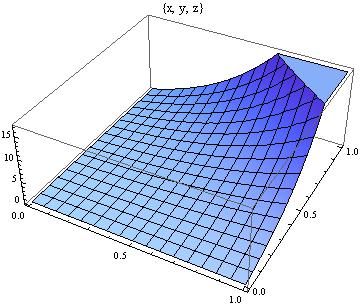
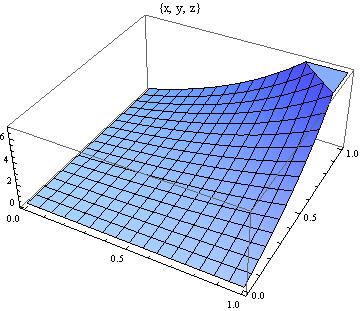
In Figure 1, we present the bivariate M-L function when $\eta=1$ and $w=0$ in (2.1).

(a) $\alpha=0.8$, $\beta=0.6$, $\delta=0.2$

(b) $\alpha=0.9$, $\beta=0.8$, $\delta=0.6$

Figure 1: The plots of the bivariate M-L function of $E_{\alpha,\beta,\delta}(u,v)$ with $\eta=1$ and varying values of $\alpha,\beta,\delta$

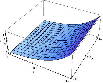
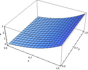
In Figure 2, we present the three-parameter M-L function when $\eta=1$ and $v=w=0$ in (2.1).

(a) $\alpha=0.6$, $\delta=0.1$

(b) $\alpha=0.9$, $\delta=0.3$

Figure 2: The plots of the three-parameter M-L function of $E_{\alpha,\delta}(u)$ with $\eta=1$ and varying values of $\alpha,\delta$

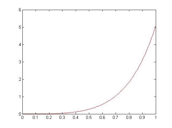
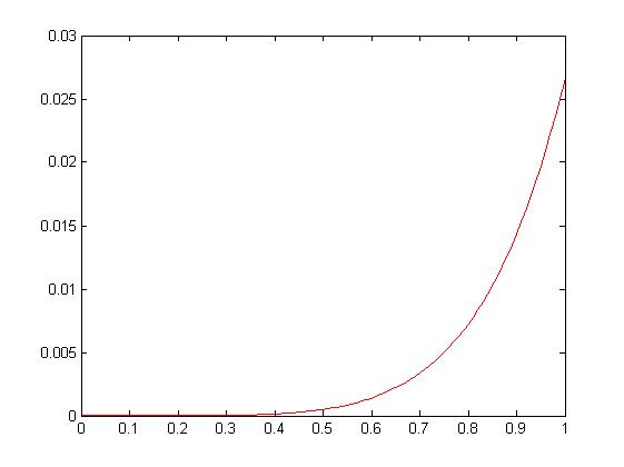
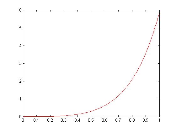
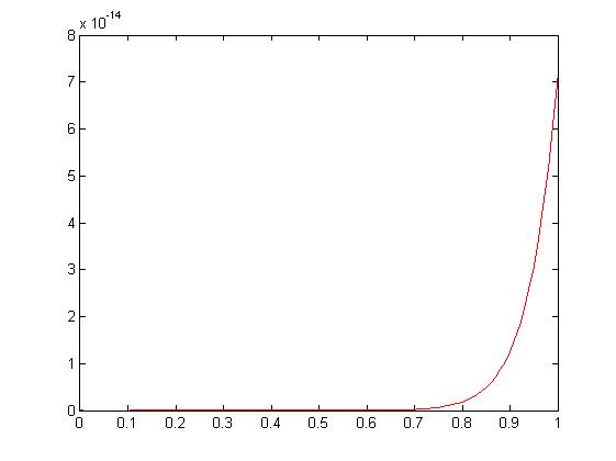
In Figure 3, we describe univariate version of the trivariate M–L function (2.3) with $\delta=\eta=1$ and different parameters $\alpha,\beta,\gamma$.

(a) $E_{1,1,1,1}^{1}(r,r,r)=\exp(3r)$

(b) $\alpha=1.5$, $\beta=1.5$, $\gamma=2.5$

(c) $\alpha=0.75$, $\beta=1$, $\gamma=1.25$

(d) $\alpha=8$, $\beta=6$, $\gamma=4$

Figure 3: The plots of the univariate version of $E_{\alpha,\beta,\gamma,1}^{1}(r^{\alpha},r^{\beta},r^{\gamma})$ with $\delta=\eta=1$ and varying $\alpha,\beta,\gamma$

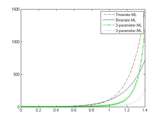
The following Figure 4 shows the comparison of new trivariate, bivariate and M–L functions with two and three parameters.

Figure 4: The comparison of various types of M–L functions

Here we provide the values of each parameter through the following table which are used in Figure 4 to compare final results for each functions.

	$E^{\eta}_{\alpha,\beta,\gamma,\delta}$	$E^{\eta}_{\alpha,\beta,\gamma}$	$E^{\eta}_{\alpha,\beta}$	$E^{\eta}_{\alpha,\beta}$
$\alpha$	$0.25$	$0.25$	$0.25$	$0.25$
$\beta$	$0.75$	$0.75$	$0.75$	$0.75$
$\gamma$	$1.5$	$1.5$	$-$	$-$
$\delta$	$1.5$	$-$	$-$	$-$
$\eta$	$1$	$1$	$1.5$	$1$

Table 1: The values of parameters for each functions

2.2 Main results and relationships

Theorem 2.1.

For $\alpha,\beta,\gamma,\delta,\eta\in\mathbb{C}$ with $\Re(\alpha)>0$, $\Re(\beta)>0$, and $\Re(\gamma)>0$, the trivariate M–L function (2.1) has the following integral representation on the complex plane:

$$E_{\alpha,\beta,\gamma,\delta}^{\eta}(u,v,w)=\frac{1}{2\pi i}\int\limits_{H}\frac{e^{\tau}\tau^{-\delta}}{(1-u\tau^{-\alpha}-v\tau^{-\beta}-w\tau^{-\gamma})^{\eta}}\mathrm{d}\tau,$$ (2.4)

where $H$ is the Hankel contour.

Proof.

Using up the well-known Hankel formula for reciprocal of the gamma function [53]:

$$\frac{1}{\Gamma(s)}=\frac{1}{2\pi i}\int\limits_{H}\tau^{-s}e^{\tau}\mathrm{d}\tau,\quad s\in\mathbb{C}.$$

Thus for $E_{\alpha,\beta,\gamma,\delta}^{\eta}(u,v,w)$, we have

$$E_{\alpha,\beta,\gamma,\delta}^{\eta}(u,v,w) =\sum_{l=0}^{\infty}\sum_{p=0}^{\infty}\sum_{k=0}^{\infty}\frac{(\eta)_{l+p+k}}{\Gamma(l\alpha+p\beta+k\gamma+\delta)}\frac{u^{l}v^{p}w^{k}}{l!p!k!}$$

$$=\frac{1}{2\pi i}\sum_{l=0}^{\infty}\sum_{p=0}^{\infty}\sum_{k=0}^{\infty}\frac{(\eta)_{l+p+k}u^{l}v^{p}w^{k}}{l!p!k!}\int\limits_{H}\tau^{-l\alpha-p\beta-k\gamma-\delta}e^{\tau}\mathrm{d}\tau$$

$$=\frac{1}{2\pi i}\int\limits_{H}e^{\tau}\tau^{-\delta}\sum_{l=0}^{\infty}\sum_{p=0}^{\infty}\sum_{k=0}^{\infty}\frac{(\eta)_{l+p+k}}{l!p!k!}\left(\frac{u}{\tau^{\alpha}}\right)^{l}\left(\frac{v}{\tau^{\beta}}\right)^{p}\left(\frac{w}{\tau^{\gamma}}\right)^{k}\mathrm{d}\tau.$$

We evaluate the triple sum in this integral above by using (2.2) and the following identity

$$\sum_{m=0}^{\infty}\frac{(\rho)_{m}}{m!}s^{m}=(1-s)^{-\rho},\rho\in\mathbb{C}$$ (2.5)

as follows:

$$\sum_{l=0}^{\infty}\sum_{p=0}^{\infty}\sum_{k=0}^{\infty}\frac{(\eta)_{l+p+k}}{l!p!k!}\left(\frac{u}{\tau^{\alpha}}\right)^{l}\left(\frac{v}{\tau^{\beta}}\right)^{p}\left(\frac{w}{\tau^{\gamma}}\right)^{k}$$

$$= \sum_{l=0}^{\infty}\sum_{p=0}^{\infty}\sum_{k=0}^{\infty}\frac{(\eta)_{l}(\eta+l)_{p}(\eta+l+p)_{k}}{l!p!k!}\left(\frac{u}{\tau^{\alpha}}\right)^{l}\left(\frac{v}{\tau^{\beta}}\right)^{p}\left(\frac{w}{\tau^{\gamma}}\right)^{k}$$

$$= \sum_{l=0}^{\infty}\frac{(\eta)_{l}}{l!}\left(\frac{u}{\tau^{\alpha}}\right)^{l}\sum_{p=0}^{\infty}\sum_{k=0}^{\infty}\frac{(\eta+l+p)_{k}(\eta+l)_{p}}{p!k!}\left(\frac{v}{\tau^{\beta}}\right)^{p}\left(\frac{w}{\tau^{\gamma}}\right)^{k}$$

$$= \sum_{l=0}^{\infty}\frac{(\eta)_{l}}{l!}\left(\frac{u}{\tau^{\alpha}}\right)^{l}\sum_{p=0}^{\infty}\sum_{k=0}^{\infty}\frac{(\eta+l)_{p+k}}{p!k!}\left(\frac{v}{\tau^{\beta}}\right)^{p}\left(\frac{w}{\tau^{\gamma}}\right)^{k}$$

$$= \sum_{l=0}^{\infty}\frac{(\eta)_{l}}{l!}\left(\frac{u}{\tau^{\alpha}}\right)^{l}\Big{(}1-\frac{v}{\tau^{\beta}}-\frac{w}{\tau^{\gamma}}\Big{)}^{-\eta-l}$$

$$= \Big{(}1-\frac{v}{\tau^{\beta}}-\frac{w}{\tau^{\gamma}}\Big{)}^{-\eta}\sum_{l=0}^{\infty}\frac{(\eta)_{l}}{l!}\Big{(}\frac{u}{\tau^{\alpha}(1-\frac{v}{\tau^{\beta}}-\frac{w}{\tau^{\gamma}})}\Big{)}^{l}$$

$$= \Big{(}1-\frac{v}{\tau^{\beta}}-\frac{w}{\tau^{\gamma}}\Big{)}^{-\eta}\Big{(}1-\frac{u}{\tau^{\alpha}(1-\frac{v}{\tau^{\beta}}-\frac{w}{\tau^{\gamma}})}\Big{)}^{-\eta}$$

$$= \Big{(}1-\frac{u}{\tau^{\alpha}}-\frac{v}{\tau^{\beta}}-\frac{w}{\tau^{\gamma}}\Big{)}^{-\eta}=\frac{1}{(1-\frac{u}{\tau^{\alpha}}-\frac{v}{\tau^{\beta}}-\frac{w}{\tau^{\gamma}})^{\eta}}.$$

Plugging this to the integral formula for $E_{\alpha,\beta,\gamma,\delta}^{\eta}(u,v,w)$ attained above, we get the desired result. ∎

Corollary 2.1.

Let $\alpha,\beta,\gamma,\delta,\eta\in\mathbb{C}$, with $\Re(\alpha)>0$, $\Re(\beta)>0$, and $\Re(\gamma)>0$, $\lambda_{1},\lambda_{2},\lambda_{3}\in\mathbb{C}$ and $r\in\mathbb{C}$. The complex integral representation for the univariate version (2.3) is defined by:

$$r^{\delta-1}E_{\alpha,\beta,\gamma,\delta}^{\eta}(\lambda_{1}r^{\alpha},\lambda_{2}r^{\beta},\lambda_{3}r^{\gamma})=\frac{1}{2\pi i}\int\limits_{H}\frac{e^{rs}s^{-\delta}}{(1-\lambda_{1}s^{-\alpha}-\lambda_{2}s^{-\beta}-\lambda_{3}s^{-\gamma})^{\eta}}\mathrm{d}s.$$

Proof.

Applying Theorem 2.1, we make use of substitution $u=\lambda_{1}r^{\alpha}$, $v=\lambda_{2}r^{\beta}$ and $w=\lambda_{3}r^{\gamma}$, we obtain:

$$E_{\alpha,\beta,\gamma,\delta}^{\eta}(\lambda_{1}r^{\alpha},\lambda_{2}r^{\beta},\lambda_{3}r^{\gamma})=\frac{1}{2\pi i}\int\limits_{H}\frac{e^{\tau}\tau^{-\delta}}{(1-\lambda_{1}\left(\frac{r}{\tau}\right)^{\alpha}-\lambda_{2}\left(\frac{r}{\tau}\right)^{\beta}-\lambda_{3}\left(\frac{r}{\tau}\right)^{\gamma})^{\eta}}\mathrm{d}\tau,$$

and

$$r^{\delta-1}E_{\alpha,\beta,\gamma,\delta}^{\eta}(\lambda_{1}r^{\alpha},\lambda_{2}r^{\beta},\lambda_{3}r^{\gamma})=\frac{1}{2\pi i}\int\limits_{H}\frac{e^{\tau}\left(\frac{r}{\tau}\right)^{\delta}}{(1-\lambda_{1}\left(\frac{r}{\tau}\right)^{\alpha}-\lambda_{2}\left(\frac{r}{\tau}\right)^{\beta}-\lambda_{3}\left(\frac{r}{\tau}\right)^{\gamma})^{\eta}}\frac{1}{r}\mathrm{d}\tau,$$

thus, substitute $s=\frac{\tau}{r}$ to get the stated result:

$$r^{\delta-1}E_{\alpha,\beta,\gamma,\delta}^{\eta}(\lambda_{1}r^{\alpha},\lambda_{2}r^{\beta},\lambda_{3}r^{\gamma})=\frac{1}{2\pi i}\int\limits_{H}\frac{e^{rs}s^{-\delta}}{(1-\lambda_{1}s^{-\alpha}-\lambda_{2}s^{-\beta}-\lambda_{3}s^{-\gamma})^{\eta}}\mathrm{d}s.$$

∎

The next results concern the Laplace integral transform of univariate formula for trivariate M–L type function (2.3).

Theorem 2.2.

For $\lambda_{i}\in\mathbb{C},i=1,2,3$, $\alpha,\beta,\gamma,\delta,\eta\in\mathbb{C}$ with $\Re(\alpha)>0$, $\Re(\beta)>0$, $\Re(\gamma)>0$, and $\Re(\delta)>0$, the following holds:

$$\mathcal{L}\left\{r^{\delta-1}E_{\alpha,\beta,\gamma,\delta}^{\eta}(\lambda_{1}r^{\alpha},\lambda_{2}r^{\beta},\lambda_{3}r^{\gamma})\right\}(s)=\frac{1}{s^{\delta}}\left(1-\frac{\lambda_{1}}{s^{\alpha}}-\frac{\lambda_{2}}{s^{\beta}}-\frac{\lambda_{3}}{s^{\gamma}}\right)^{-\eta},\quad\Re(s)>0.$$

Proof.

Since the triple series is locally and uniformly convergent, we can integrate it term by term. The Laplace integral transform of a power function is defined by

$$\mathcal{L}\left\{\frac{r^{l-1}}{\Gamma(l)}\right\}(s)=\frac{1}{s^{l}},\quad\Re(l)>-1.$$

Therefore, by using (2.5) for the trivariate Mittag-Leffler type function we have:

$$\mathcal{L}\left\{r^{\delta-1}E_{\alpha,\beta,\gamma,\delta}^{\eta}(\lambda_{1}r^{\alpha},\lambda_{2}r^{\beta},\lambda_{3}r^{\gamma})\right\}(s) =\sum_{l=0}^{\infty}\sum_{p=0}^{\infty}\sum_{k=0}^{\infty}\frac{(\eta)_{l+p+k}}{\Gamma(l\alpha+p\beta+k\gamma+\delta)}\frac{\lambda_{1}^{l}\lambda_{2}^{p}\lambda_{3}^{k}}{l!p!k!}\mathcal{L}\left\{r^{l\alpha+p\beta+k\gamma+\delta-1}\right\}(s)$$

$$=\frac{1}{s^{\delta}}\sum_{l=0}^{\infty}\sum_{p=0}^{\infty}\sum_{k=0}^{\infty}\frac{(\eta)_{l+p+k}}{l!p!k!}\left(\frac{\lambda_{1}}{s^{\alpha}}\right)^{l}\left(\frac{\lambda_{2}}{s^{\beta}}\right)^{p}\left(\frac{\lambda_{3}}{s^{\gamma}}\right)^{k}$$

$$=\frac{1}{s^{\delta}}\sum_{l=0}^{\infty}\sum_{p=0}^{\infty}\frac{(\eta)_{l+p}}{l!p!}\left(\frac{\lambda_{1}}{s^{\alpha}}\right)^{l}\left(\frac{\lambda_{2}}{s^{\beta}}\right)^{p}\sum_{k=0}^{\infty}\frac{(\eta+l+p)_{k}}{k!}\left(\frac{\lambda_{3}}{s^{\gamma}}\right)^{k}$$

$$=\frac{1}{s^{\delta}}\left(1-\frac{\lambda_{3}}{s^{\gamma}}\right)^{-\eta}\sum_{l=0}^{\infty}\frac{(\eta)_{l}}{l!}\left(\frac{\lambda_{1}}{s^{\alpha}}\right)^{l}\left(1-\frac{\lambda_{3}}{s^{\gamma}}\right)^{-l}\sum_{p=0}^{\infty}\frac{(\eta+l)_{p}}{p!}\left(\frac{\lambda_{2}}{s^{\beta}}\right)^{p}\left(1-\frac{\lambda_{3}}{s^{\gamma}}\right)^{-p}$$

$$=\frac{1}{s^{\delta}}\left(1-\frac{\lambda_{3}}{s^{\gamma}}\right)^{-\eta}\left(1-\frac{\lambda_{2}}{s^{\beta}}\left(1-\frac{\lambda_{3}}{s^{\gamma}}\right)^{-1}\right)^{-\eta}\sum_{l=0}^{\infty}\frac{(\eta)_{l}}{l!}\left(\frac{\lambda_{1}}{s^{\alpha}}\right)^{l}\left(1-\frac{\lambda_{3}}{s^{\gamma}}\right)^{-l}\left(1-\frac{\lambda_{2}}{s^{\beta}}\left(1-\frac{\lambda_{3}}{s^{\gamma}}\right)^{-1}\right)^{-l}$$

$$=\frac{1}{s^{\delta}}\left(1-\frac{\lambda_{2}}{s^{\beta}}-\frac{\lambda_{3}}{s^{\gamma}}\right)^{-\eta}\sum_{l=0}^{\infty}\frac{(\eta)_{l}}{l!}\left(\frac{\lambda_{1}}{s^{\alpha}}\left(1-\frac{\lambda_{2}}{s^{\beta}}-\frac{\lambda_{3}}{s^{\gamma}}\right)^{-1}\right)^{l}$$

$$=\frac{1}{s^{\delta}}\left(1-\frac{\lambda_{2}}{s^{\beta}}-\frac{\lambda_{3}}{s^{\gamma}}\right)^{-\eta}\left(1-\frac{\lambda_{1}}{s^{\alpha}}\left(1-\frac{\lambda_{2}}{s^{\beta}}-\frac{\lambda_{3}}{s^{\gamma}}\right)^{-1}\right)^{-\eta}$$

$$=\frac{1}{s^{\delta}}\left(1-\frac{\lambda_{1}}{s^{\alpha}}-\frac{\lambda_{2}}{s^{\beta}}-\frac{\lambda_{3}}{s^{\gamma}}\right)^{-\eta}.$$

Note that we have need of extra conditions on $s$:

$$\left\lvert\frac{\lambda_{3}}{s^{\gamma}}\right\rvert<1,\quad\left\lvert\frac{\lambda_{2}}{s^{\beta}}\left(1-\frac{\lambda_{3}}{s^{\gamma}}\right)^{-1}\right\rvert<1\quad\text{and}\quad\left\lvert\frac{\lambda_{1}}{s^{\alpha}}\left(1-\frac{\lambda_{2}}{s^{\beta}}-\frac{\lambda_{3}}{s^{\gamma}}\right)^{-1}\right\rvert<1,$$

for proper convergence of the series. However, these conditions can be reduced according to the analytic continuation. Therefore, this gives the desired result for arbitrary $s\in\mathbb{C}$ whenever $\Re(s)>0$. ∎

Next we prove a result of convolution on trivariate Mittag-Leffler type functions which is related to above theorem directly.

Theorem 2.3.

Let $\lambda_{i}\in\mathbb{C},i=1,2,3$, $\alpha,\beta,\gamma,\delta_{1},\delta_{2},\eta_{1},\eta_{2}\in\mathbb{C}$ with $\Re(\alpha)>0$, $\Re(\beta)>0$, $\Re(\gamma)>0$ and $\Re(\delta_{j})>0,j=1,2$. Then the next result yields:

$$\left(r^{\delta_{1}-1}E_{\alpha,\beta,\gamma,\delta_{1}}^{\eta_{1}}(\lambda_{1}r^{\alpha},\lambda_{2}r^{\beta},\lambda_{3}r^{\gamma})\right) \ast\left(r^{\delta_{2}-1}E_{\alpha,\beta,\gamma,\delta_{2}}^{\eta_{2}}(\lambda_{1}r^{\alpha},\lambda_{2}r^{\beta},\lambda_{3}r^{\gamma})\right)$$

$$=r^{\delta_{1}+\delta_{2}-1}E_{\alpha,\beta,\gamma,\delta_{1}+\delta_{2}}^{\eta_{1}+\eta_{2}}(\lambda_{1}r^{\alpha},\lambda_{2}r^{\beta},\lambda_{3}r^{\gamma}).$$ (2.6)

Proof.

By using the theorem of convolution for the Laplace transformation and Theorem 2.2, we get

$$\mathcal{L}\Biggl{\{}\left(r^{\delta_{1}-1}E_{\alpha,\beta,\gamma,\delta_{1}}^{\eta_{1}}(\lambda_{1}r^{\alpha},\lambda_{2}r^{\beta},\lambda_{3}r^{\gamma})\right)\ast\left(r^{\delta_{2}-1}E_{\alpha,\beta,\gamma,\delta_{2}}^{\eta_{2}}(\lambda_{1}r^{\alpha},\lambda_{2}r^{\beta},\lambda_{3}r^{\gamma})\right)\Biggr{\}}(s)$$

$$= \mathcal{L}\left\{r^{\delta_{1}-1}E_{\alpha,\beta,\gamma,\delta_{1}}^{\eta_{1}}(\lambda_{1}r^{\alpha},\lambda_{2}r^{\beta},\lambda_{3}r^{\gamma})\right\}(s)\mathcal{L}\left\{r^{\delta_{2}-1}E_{\alpha,\beta,\gamma,\delta_{2}}^{\eta_{2}}(\lambda_{1}r^{\alpha},\lambda_{2}r^{\beta},\lambda_{3}r^{\gamma})\right\}(s)$$

$$= \frac{1}{s^{\delta_{1}}}\left(1-\frac{\lambda_{1}}{s^{\alpha}}-\frac{\lambda_{2}}{s^{\beta}}-\frac{\lambda_{3}}{s^{\gamma}}\right)^{-\eta_{1}}\frac{1}{s^{\delta_{2}}}\left(1-\frac{\lambda_{1}}{s^{\alpha}}-\frac{\lambda_{2}}{s^{\beta}}-\frac{\lambda_{3}}{s^{\gamma}}\right)^{-\eta_{2}}$$

$$= \frac{1}{s^{\delta_{1}+\delta_{2}}}\left(1-\frac{\lambda_{1}}{s^{\alpha}}-\frac{\lambda_{2}}{s^{\beta}}-\frac{\lambda_{3}}{s^{\gamma}}\right)^{-(\eta_{1}+\eta_{2})}$$

$$= \mathcal{L}\left\{r^{\delta_{1}+\delta_{2}-1}E_{\alpha,\beta,\gamma,\delta_{1}+\delta_{2}}^{\eta_{1}+\eta_{2}}(\lambda_{1}r^{\alpha},\lambda_{2}r^{\beta},\lambda_{3}r^{\gamma})\right\}(s).$$

Taking inverse Laplace transform both sides to the above expression, we acquire the desired result. ∎

3 Fractional calculus of trivariate M–L function

In this section firstly, we investigate $n$-th order derivative and integration of a newly defined trivariate Mittag-Leffler type function. Next using these results we will investigate fractional derivative and fractional integral of a trivarivate M–L function in R–L and Caputo senses.

Theorem 3.1.

Let $\alpha,\beta,\gamma,\delta,\eta,\lambda_{i}\in\mathbb{C}$ with $\Re(\alpha),\Re(\beta)$,and $\Re(\gamma)>0,i=1,2,3$. Then for arbitrary $n\in\mathbb{N}$, the following formula holds true:

$$\left(\frac{d}{dr}\right)^{n}\left[r^{\delta-1}E_{\alpha,\beta,\gamma,\delta}^{\eta}(\lambda_{1}r^{\alpha},\lambda_{2}r^{\beta},\lambda_{3}r^{\gamma})\right]=r^{\delta-n-1}E_{\alpha,\beta,\gamma,\delta-n}^{\eta}(\lambda_{1}r^{\alpha},\lambda_{2}r^{\beta},\lambda_{3}r^{\gamma}).$$ (3.1)

Proof.

By using (2.3) and differentiating term by term under the summation signs, we acquire that

$$\left(\frac{d}{dr}\right)^{n}\left[r^{\delta-1}E_{\alpha,\beta,\gamma,\delta}^{\eta}(\lambda_{1}r^{\alpha},\lambda_{2}r^{\beta},\lambda_{3}r^{\gamma})\right]$$

$$=\sum_{l=0}^{\infty}\sum_{p=0}^{\infty}\sum_{k=0}^{\infty}\frac{(\eta)_{l+p+k}}{\Gamma(l\alpha+p\beta+k\gamma+\delta)}\frac{\lambda_{1}^{l}\lambda_{2}^{p}\lambda_{3}^{k}}{l!p!k!}\left(\frac{d}{dr}\right)^{n}[r^{l\alpha+p\beta+k\gamma+\delta-1}]$$

$$=\sum_{l=0}^{\infty}\sum_{p=0}^{\infty}\sum_{k=0}^{\infty}\frac{(\eta)_{l+p+k}}{\Gamma(l\alpha+p\beta+k\gamma+\delta)}\frac{\lambda_{1}^{l}\lambda_{2}^{p}\lambda_{3}^{k}}{l!p!k!}\frac{\Gamma(l\alpha+p\beta+k\gamma+\delta)}{\Gamma(l\alpha+p\beta+k\gamma+\delta-n)}[r^{l\alpha+p\beta+k\gamma+\delta-n-1}]$$

$$=\sum_{l=0}^{\infty}\sum_{p=0}^{\infty}\sum_{k=0}^{\infty}\frac{(\eta)_{l+p+k}}{\Gamma(l\alpha+p\beta+k\gamma+\delta-n)}\frac{\lambda_{1}^{l}\lambda_{2}^{p}\lambda_{3}^{k}}{l!p!k!}r^{l\alpha+p\beta+k\gamma+\delta-n-1}$$

$$=r^{\delta-n-1}E_{\alpha,\beta,\gamma,\delta-n}^{\eta}(\lambda_{1}r^{\alpha},\lambda_{2}r^{\beta},\lambda_{3}r^{\gamma}),$$

which proves (3.1). ∎

Corollary 3.1.

Let $\alpha,\beta,\gamma,\delta,\eta,\lambda_{i}\in\mathbb{C}$ with $\Re(\alpha),\Re(\beta),\Re(\gamma),\Re(\delta)>0,i=1,2,3$. Then the following holds:

$$\int\limits_{0}^{r}s^{\delta-1}E_{\alpha,\beta,\gamma,\delta}^{\eta}(\lambda_{1}s^{\alpha},\lambda_{2}s^{\beta},\lambda_{3}s^{\gamma})\mathrm{d}s=r^{\delta}E_{\alpha,\beta,\gamma,\delta+1}^{\eta}(\lambda_{1}r^{\alpha},\lambda_{2}r^{\beta},\lambda_{3}r^{\gamma}).$$

Next we consider the R–L type fractional integral and derivative of a trivariate M–L function of order $\alpha\in\mathbb{C}$ where $\Re(\alpha)>0$.

Theorem 3.2.

Let $a\in\mathbb{R_{+}},\nu,\alpha,\beta,\gamma,\delta,\eta,\lambda_{i}\in\mathbb{C}$ with $\Re(\nu),\Re(\alpha),\Re(\beta),\Re(\gamma),\Re(\delta)>0,i=1,2,3$.Then for $r,y>a$, there holds the following relations:

$$\left(\prescript{}{}{I}^{\nu}_{a_{+}}\left((r-a)^{\delta-1}E_{\alpha,\beta,\gamma,\delta}^{\eta}(\lambda_{1}(r-a)^{\alpha},\lambda_{2}(r-a)^{\beta},\lambda_{3}(r-a)^{\gamma})\right)\right)(y)$$

$$=(y-a)^{\delta+\nu-1}E_{\alpha,\beta,\gamma,\delta+\nu}^{\eta}(\lambda_{1}(y-a)^{\alpha},\lambda_{2}(y-a)^{\beta},\lambda_{3}(y-a)^{\gamma}),$$ (3.2)

and

$$\left(\prescript{}{}{D}^{\nu}_{a_{+}}\left((r-a)^{\delta-1}E_{\alpha,\beta,\gamma,\delta}^{\eta}(\lambda_{1}(r-a)^{\alpha},\lambda_{2}(r-a)^{\beta},\lambda_{3}(r-a)^{\gamma})\right)\right)(y)$$

$$=(y-a)^{\delta-\nu-1}E_{\alpha,\beta,\gamma,\delta-\nu}^{\eta}(\lambda_{1}(y-a)^{\alpha},\lambda_{2}(y-a)^{\beta},\lambda_{3}(y-a)^{\gamma}).$$ (3.3)

Proof.

By the aid of formulas (1.10) and (2.3) with the following relation ([41], Eq. (2.44))

$$\left(\prescript{}{}{I}^{\nu}_{a_{+}}(r-a)^{\gamma-1}\right)(y)=\frac{\Gamma(\gamma)}{\Gamma(\gamma+\nu)}(y-a)^{\gamma+\nu-1},$$

where $\alpha,\beta\in\mathbb{C}$ with $\Re(\alpha),\Re(\beta)>0$, leads to

$$\left(\prescript{}{}{I}^{\nu}_{a_{+}}\left((r-a)^{\delta-1}E_{\alpha,\beta,\gamma,\delta}^{\eta}(\lambda_{1}(r-a)^{\alpha},\lambda_{2}(r-a)^{\beta},\lambda_{3}(r-a)^{\gamma})\right)\right)(y)$$

$$=\sum_{l=0}^{\infty}\sum_{p=0}^{\infty}\sum_{k=0}^{\infty}\frac{(\eta)_{l+p+k}}{\Gamma(l\alpha+p\beta+k\gamma+\delta)}\frac{\lambda_{1}^{l}\lambda_{2}^{p}\lambda_{3}^{k}}{l!p!k!}\left(\prescript{}{}{I}^{\nu}_{a_{+}}(r^{l\alpha+p\beta+k\gamma+\delta-1})\right)(y)$$

$$=(y-a)^{\delta+\nu-1}E_{\alpha,\beta,\gamma,\delta+\nu}^{\eta}(\lambda_{1}(y-a)^{\alpha},\lambda_{2}(y-a)^{\beta},\lambda_{3}(y-a)^{\gamma}),\quad\text{for}\quad r,y>a.$$

To prove (3.2), we are using the results of (1.13) and (2.3) obtain that

$$\left(\prescript{}{}{D}^{\nu}_{a_{+}}\left((r-a)^{\delta-1}E_{\alpha,\beta,\gamma,\delta}^{\eta}(\lambda_{1}(r-a)^{\alpha},\lambda_{2}(r-a)^{\beta},\lambda_{3}(r-a)^{\gamma})\right)\right)(y)$$

$$= \left(\frac{d}{dy}\right)^{n}\left(\prescript{}{}{I}^{n-\nu}_{a_{+}}\left((r-a)^{\delta-1}E_{\alpha,\beta,\gamma,\delta}^{\eta}(\lambda_{1}(r-a)^{\alpha},\lambda_{2}(r-a)^{\beta},\lambda_{3}(r-a)^{\gamma})\right)\right)(y)$$

$$= \left(\frac{d}{dy}\right)^{n}(y-a)^{\delta+n-\nu-1}E_{\alpha,\beta,\gamma,\delta+n-\nu}^{\eta}(\lambda_{1}(y-a)^{\alpha},\lambda_{2}(y-a)^{\beta},\lambda_{3}(y-a)^{\gamma}).$$

Result (3.2) is obtained by the virtue of (3.1). ∎

Next we will consider the fractional derivative of M–L type function with three variable in Caputo’s sense.

Lemma 3.1.

Suppose that $\gamma,\nu\in\mathbb{C}$ with $\Re(\nu)\geq 0$. Then Caputo fractional differentiation of $\frac{(r-a)^{\gamma}}{\Gamma(\gamma+1)}$ is given by:

$$\prescript{C}{}{D}^{\nu}_{a_{+}}\left(\frac{(r-a)^{\gamma}}{\Gamma(\gamma+1)}\right)(y)=\frac{(y-a)^{\gamma-\nu}}{\Gamma(\gamma-\nu+1)},\quad r,y>a.$$

Proof.

Let $n\coloneqq\lfloor\Re(\nu)\rfloor+1$, $\Re(\nu)\geq 0$. Then we have:

$$\prescript{C}{}{D}^{\nu}_{a_{+}}\left(\frac{(r-a)^{\gamma}}{\Gamma(\gamma+1)}\right)(y) =\prescript{}{}{I}^{n-\nu}_{a_{+}}\left(\frac{d^{n}}{dr^{n}}\frac{(r-a)^{\gamma}}{\Gamma(\gamma+1)}\right)(y)=\prescript{}{}{I}^{n-\nu}_{a_{+}}\left(\frac{(r-a)^{\gamma-n}}{\Gamma(\gamma-n+1)}\right)(y)$$

$$=\frac{1}{\Gamma(n-\nu)}\int_{a}^{y}(y-s)^{n-\nu-1}\frac{(s-a)^{\gamma-n}}{\Gamma(\gamma-n+1)}\mathrm{d}s$$

$$\overset{u=\frac{y-s}{y-a}}{=}\frac{1}{\Gamma(n-\nu)}\frac{(y-a)^{\gamma-\nu}}{\Gamma(\gamma-n+1)}\mathbf{B}(n-\nu,\gamma-n+1)$$

$$=\frac{(y-a)^{\gamma-\nu}}{\Gamma(\gamma-\nu+1)}.$$

∎

Theorem 3.3.

Let $\lambda_{i}\in\mathbb{C},i=1,2,3$, $\nu,\alpha,\beta,\gamma,\delta,\eta\in\mathbb{C}$ with $\Re(\nu)\geq 0$,$\Re(\alpha)>0$, $\Re(\beta)>0$, $\Re(\gamma)>0$ and $\Re(\delta)>0$. Then the fractional differentiation of the function (2.3) in Caputo sense is given by:

$$\left(\prescript{C}{}{D}^{\nu}_{a_{+}}\left((r-a)^{\delta-1}E_{\alpha,\beta,\gamma,\delta}^{\eta}(\lambda_{1}(r-a)^{\alpha},\lambda_{2}(r-a)^{\beta},\lambda_{3}(r-a)^{\gamma})\right)\right)(y)$$

$$=(y-a)^{\delta-\nu-1}E_{\alpha,\beta,\gamma,\delta-\nu}^{\eta}(\lambda_{1}(y-a)^{\alpha},\lambda_{2}(y-a)^{\beta},\lambda_{3}(y-a)^{\gamma}),\quad r,y>a.$$

Proof.

According to Lemma 3.1, fractionally differentiating the series (2.3) term by term gives:

$$\left(\prescript{C}{}{D}^{\nu}_{a_{+}}\left((r-a)^{\delta-1}E_{\alpha,\beta,\gamma,\delta}^{\eta}(\lambda_{1}(r-a)^{\alpha},\lambda_{2}(r-a)^{\beta},\lambda_{3}(r-a)^{\gamma})\right)\right)(y)$$

$$=\sum_{l=0}^{\infty}\sum_{p=0}^{\infty}\sum_{k=0}^{\infty}\frac{(\eta)_{l+p+k}}{l!p!k!}\prescript{C}{}{D}^{\nu}_{a_{+}}\left(\frac{(r-a)^{l\alpha+p\beta+k\gamma+\delta-1}}{\Gamma(l\alpha+p\beta+k\gamma+\delta)}\right)(y)$$

$$=(y-a)^{\delta-\nu-1}\sum_{l=0}^{\infty}\sum_{p=0}^{\infty}\sum_{k=0}^{\infty}\frac{(\eta)_{l+p+k}}{\Gamma(l\alpha+p\beta+k\gamma+\delta-\nu)}\frac{(\lambda_{1}(y-a)^{\alpha})^{l}}{l!}\frac{(\lambda_{2}(y-a)^{\beta})^{n}}{p!}\frac{(\lambda_{3}(y-a)^{\gamma})^{k}}{k!}$$

$$=(y-a)^{\delta-\nu-1}E_{\alpha,\beta,\gamma,\delta-\nu}^{\eta}(\lambda_{1}(y-a)^{\alpha},\lambda_{2}(y-a)^{\beta},\lambda_{3}(y-a)^{\gamma}),$$

where the result is also uniformly convergent. ∎

4 Multi-term fractional differential equations

In this section, we derive an explicit solutions to homogeneous and inhomogenous multi-term FDEs.

4.1 Analytical representation of solution to the homogeneous multi-term fractional differential equation

In this subsection, we consider the initial value problem for linear homogeneous FDE with three independent fractional orders:

$$\left(\prescript{C}{}{D}^{\alpha}_{0+}y\right)(r)-\lambda_{3}\left(\prescript{C}{}{D}^{\beta}_{0+}y\right)(r)-\lambda_{2}\left(\prescript{C}{}{D}^{\gamma}_{0+}y\right)(r)-\lambda_{1}y(r)=0,$$ (4.1)

with initial condition $y(0)=y_{0}$.

The following lemma and trinomial identity will be of significance for our results in the next theorem.

Lemma 4.1.

For any parameters $\rho,\alpha,\beta,\gamma,\delta,\lambda_{1},\lambda_{2},\lambda_{3}\in\mathbb{R}$ satisfying $\rho\geq 0,\alpha,\beta,\gamma>0$ and $\delta-1>\lfloor\rho\rfloor$, we have:

$$\left(\prescript{C}{}{D}^{\rho}_{0+}\Big{[}r^{\delta-1}E_{\alpha,\beta,\gamma,\delta}(\lambda_{1}r^{\alpha},\lambda_{2}r^{\beta},\lambda_{3}r^{\gamma})\Big{]}\right)(y)=y^{\delta-\rho-1}E_{\alpha,\beta,\gamma,\delta-\rho}(\lambda_{1}y^{\alpha},\lambda_{2}y^{\beta},\lambda_{3}y^{\gamma}),\quad r,y>0.$$

Proof.

From Lemma 3.1, we have

$$\left(\prescript{C}{}{D}^{\nu}_{0+}(\frac{r^{\mu}}{\Gamma(\mu+1)})\right)(y)=\frac{y^{\mu-\nu}}{\Gamma(\mu-\nu+1)},\quad\mu>\lfloor\nu\rfloor,\quad r,y>0.$$

Therefore, in accordance with (4.1), fractionally differentiating the function (2.3) term by term :

$$\left(\prescript{C}{}{D}^{\rho}_{0+}\left[\sum_{l=0}^{\infty}\sum_{p=0}^{\infty}\sum_{k=0}^{\infty}\frac{(l+p+k)!\lambda_{1}^{l}\lambda_{2}^{p}\lambda_{3}^{k}r^{l\alpha+p\beta+k\gamma+\delta-1}}{\Gamma(l\alpha+p\beta+k\gamma+\delta)l!p!k!}\right]\right)(y)$$

$$=\sum_{l=0}^{\infty}\sum_{p=0}^{\infty}\sum_{k=0}^{\infty}\frac{(l+p+k)!\lambda_{1}^{l}\lambda_{2}^{p}\lambda_{3}^{k}y^{l\alpha+p\beta+k\gamma+\delta-\rho-1}}{\Gamma(l\alpha+p\beta+k\gamma+\delta-\rho)l!p!k!}$$

$$=y^{\delta-\rho-1}E_{\alpha,\beta,\gamma,\delta-\rho}(\lambda_{1}y^{\alpha},\lambda_{2}y^{\beta},\lambda_{3}y^{\gamma}),\quad r,y>0.$$

∎

Pascal’s tetrahedron. If $q\geq 1$, $lpk\neq 0$, then

$$\binom{q}{l,p,k}=\binom{q-1}{l-1,p,k}+\binom{q-1}{l,p-1,k}+\binom{q-1}{l,p,k-1}.$$ (4.2)

In other case, the so-called Pascal’s rule holds, for example $k=0$ and $lp\neq 0$

$$\binom{q}{l,p}=\binom{q-1}{l-1,p}+\binom{q-1}{l,p-1}.$$

If $q=l+p+k$, then trinomial coefficient is defined by

$$\binom{l+p+k}{l,p,k}=\frac{(l+p+k)!}{l!p!k!}.$$

Theorem 4.1.

The univariate form (2.3) of the trivariate M–L function (2.1) with $\eta=1$, gives a solution

$$y(r)=\left(1+\lambda_{1}r^{\alpha}E_{\alpha,\alpha-\gamma,\alpha-\beta,\alpha+1}(\lambda_{1}r^{\alpha},\lambda_{2}r^{\alpha-\gamma},\lambda_{3}r^{\alpha-\beta})\right)y_{0},$$ (4.3)

for intial value problem for the multi-term differential equation involving three independent fractional orders (4.1).

Proof.

It should be noted that the Caputo derivative of constant function is equal to zero. We will apply Lemma 4.1 to show that $y(r)$ is a solution of (4.1). Starting from the series (2.3), we evaluate the fractional differ-integrals of $y(r)$ as below:

$$\left(\prescript{C}{}{D}^{\alpha}_{0+}y\right)(r) =\prescript{C}{}{D}^{\alpha}_{0+}\left(1+\sum_{l=0}^{\infty}\sum_{p=0}^{\infty}\sum_{k=0}^{\infty}\binom{l+p+k}{l,p,k}\frac{\lambda_{1}^{l+1}\lambda_{2}^{p}\lambda_{3}^{k}r^{l\alpha+p(\alpha-\gamma)+k(\alpha-\beta)+\alpha}}{\Gamma(l\alpha+p(\alpha-\gamma)+k(\alpha-\beta)+\alpha+1)}\right)y_{0}$$

$$=\sum_{l=0}^{\infty}\sum_{p=0}^{\infty}\sum_{k=0}^{\infty}\binom{l+p+k}{l,p,k}\lambda_{1}^{l+1}\lambda_{2}^{p}\lambda_{3}^{k}\prescript{C}{}{D}^{\alpha}_{0+}\left(\frac{r^{l\alpha+p(\alpha-\gamma)+k(\alpha-\beta)+\alpha}}{\Gamma(l\alpha+p(\alpha-\gamma)+k(\alpha-\beta)+\alpha+1)}\right)y_{0}$$

$$=\sum_{l=0}^{\infty}\sum_{p=0}^{\infty}\sum_{k=0}^{\infty}\binom{l+p+k}{l,p,k}\frac{\lambda_{1}^{l+1}\lambda_{2}^{p}\lambda_{3}^{k}r^{l\alpha+p(\alpha-\gamma)+k(\alpha-\beta)}}{\Gamma(l\alpha+p(\alpha-\gamma)+k(\alpha-\beta)+1)}y_{0}$$

$$=\Big{(}\lambda_{1} +\sum_{l=1}^{\infty}\sum_{p=0}^{\infty}\sum_{k=0}^{\infty}\binom{l+p+k-1}{l-1,p,k}\frac{\lambda_{1}^{l+1}\lambda_{2}^{p}\lambda_{3}^{k}r^{l\alpha+p(\alpha-\gamma)+k(\alpha-\beta)}}{\Gamma(l\alpha+p(\alpha-\gamma)+k(\alpha-\beta)+1)}$$

$$+\sum_{l=0}^{\infty}\sum_{p=1}^{\infty}\sum_{k=0}^{\infty}\binom{l+p+k-1}{l,p-1,k}\frac{\lambda_{1}^{l+1}\lambda_{2}^{p}\lambda_{3}^{k}r^{l\alpha+p(\alpha-\gamma)+k(\alpha-\beta)}}{\Gamma(l\alpha+p(\alpha-\gamma)+k(\alpha-\beta)+1)}$$

$$+\sum_{l=0}^{\infty}\sum_{p=0}^{\infty}\sum_{k=1}^{\infty}\binom{l+p+k-1}{l,p,k-1}\frac{\lambda_{1}^{l+1}\lambda_{2}^{p}\lambda_{3}^{k}r^{l\alpha+p(\alpha-\gamma)+k(\alpha-\beta)}}{\Gamma(l\alpha+p(\alpha-\gamma)+k(\alpha-\beta)+1)}\Big{)}y_{0}$$

Similarly, we have :

$$\lambda_{3}\left(\prescript{C}{}{D}^{\beta}_{0+}y\right)(r) =\lambda_{3}\prescript{C}{}{D}^{\beta}_{0+}\Big{(}1+\lambda_{1}r^{\alpha}E_{\alpha,\alpha-\gamma,\alpha-\beta,\alpha+1}(\lambda_{1}r^{\alpha},\lambda_{2}r^{\alpha-\gamma},\lambda_{3}r^{\alpha-\beta})\Big{)}y_{0}$$

$$=\lambda_{1}\lambda_{3}r^{\alpha-\beta}E_{\alpha,\alpha-\gamma,\alpha-\beta,\alpha-\beta+1}(\lambda_{1}r^{\alpha},\lambda_{2}r^{\alpha-\gamma},\lambda_{3}r^{\alpha-\beta})y_{0}$$

$$=\sum_{l=0}^{\infty}\sum_{p=0}^{\infty}\sum_{k=0}^{\infty}\binom{l+p+k}{l,p,k}\frac{\lambda_{1}^{l+1}\lambda_{2}^{p}\lambda_{3}^{k+1}r^{l\alpha+p(\alpha-\gamma)+(k+1)(\alpha-\beta)}}{\Gamma(l\alpha+p(\alpha-\gamma)+(k+1)(\alpha-\beta)+1)}y_{0}$$

$$=\sum_{l=0}^{\infty}\sum_{p=0}^{\infty}\sum_{k=1}^{\infty}\binom{l+p+k-1}{l,p,k-1}\frac{\lambda_{1}^{l+1}\lambda_{2}^{p}\lambda_{3}^{k}r^{l\alpha+p(\alpha-\gamma)+k(\alpha-\beta)}}{\Gamma(l\alpha+p(\alpha-\gamma)+k(\alpha-\beta)+1)}y_{0},$$

and

$$\lambda_{2}\left(\prescript{C}{}{D}^{\gamma}_{0+}y\right)(r) =\lambda_{2}\prescript{C}{}{D}^{\gamma}_{0+}\Big{(}1+\lambda_{1}r^{\alpha}E_{\alpha,\alpha-\gamma,\alpha-\beta,\alpha+1}(\lambda_{1}r^{\alpha},\lambda_{2}r^{\alpha-\gamma},\lambda_{3}r^{\alpha-\beta})\Big{)}y_{0}$$

$$=\lambda_{1}\lambda_{2}r^{\alpha-\gamma}E_{\alpha,\alpha-\gamma,\alpha-\beta,\alpha-\gamma+1}(\lambda_{1}r^{\alpha},\lambda_{2}r^{\alpha-\gamma},\lambda_{3}r^{\alpha-\gamma})y_{0}$$

$$=\sum_{l=0}^{\infty}\sum_{p=0}^{\infty}\sum_{k=0}^{\infty}\binom{l+p+k}{l,p,k}\frac{\lambda_{1}^{l+1}\lambda_{2}^{p+1}\lambda_{3}^{k}r^{l\alpha+(p+1)(\alpha-\gamma)+k(\alpha-\beta)}}{\Gamma(l\alpha+(p+1)(\alpha-\gamma)+k(\alpha-\beta)+1)}y_{0}$$

$$=\sum_{l=0}^{\infty}\sum_{p=1}^{\infty}\sum_{k=0}^{\infty}\binom{l+p+k-1}{l,p-1,k}\frac{\lambda_{1}^{l+1}\lambda_{2}^{p}\lambda_{3}^{k}r^{l\alpha+p(\alpha-\gamma)+k(\alpha-\beta)}}{\Gamma(l\alpha+p(\alpha-\gamma)+k(\alpha-\beta)+1)}y_{0},$$

and

$$\lambda_{1}y(r) =\lambda_{1}\left(1+\lambda_{1}r^{\alpha}E_{\alpha,\alpha-\gamma,\alpha-\beta,\alpha+1}(\lambda_{1}r^{\alpha},\lambda_{2}r^{\alpha-\gamma},\lambda_{3}r^{\alpha-\beta})\right)y_{0}$$

$$=\left(\lambda_{1}+\sum_{l=0}^{\infty}\sum_{p=0}^{\infty}\sum_{k=0}^{\infty}\binom{l+p+k}{l,p,k}\frac{\lambda_{1}^{l+2}\lambda_{2}^{p}\lambda_{3}^{k}r^{l\alpha+p(\alpha-\gamma)+k(\alpha-\beta)+\alpha}}{\Gamma(l\alpha+p(\alpha-\gamma)+k(\alpha-\beta)+\alpha+1)}\right)y_{0}$$

$$=\left(\lambda_{1}+\sum_{l=1}^{\infty}\sum_{p=0}^{\infty}\sum_{k=0}^{\infty}\binom{l+p+k-1}{l-1,p,k}\frac{\lambda_{1}^{l+1}\lambda_{2}^{p}\lambda_{3}^{k}r^{l\alpha+p(\alpha-\gamma)+k(\alpha-\beta)}}{\Gamma(l\alpha+p(\alpha-\gamma)+k(\alpha-\beta)+1)}\right)y_{0}.$$

Taking a linear combination, we find

$$\left(\prescript{C}{}{D}^{\alpha}_{0+}y\right)(r)-\lambda_{3}\left(\prescript{C}{}{D}^{\beta}_{0+}y\right)(r)-\lambda_{2}\left(\prescript{C}{}{D}^{\gamma}_{0+}y\right)(r)-\lambda_{1}y(r)=0.$$

which satisfying the initial data $y(0)=y_{0}$. Thus, the results are proved. ∎

Remark 4.1.

The Cauchy problem (4.1) has a solution given by using Fox-Wright functions (1.9)

$$y(r) =\sum_{d=0}^{\infty}\Big{(}\sum_{l+p=d}\Big{)}\frac{\lambda^{l}_{1}\lambda^{p}_{2}}{l!p!}r^{(\alpha-\beta)d+\beta l+(\beta-\gamma)p}\Biggl{\{}\prescript{}{1}{}{\Psi}_{1}\left[\begin{array}[]{ccc}(d+1,1)\\ ((\alpha-\beta)d+\beta l+(\beta-\gamma)p+1,\alpha-\beta)\end{array}\Big{|}\lambda_{3}r^{\alpha-\beta}\right]$$

$$-\lambda_{3}r^{\alpha-\beta}\prescript{}{1}{}{\Psi}_{1}\left[\begin{array}[]{ccc}(d+1,1)\\ ((\alpha-\beta)(d+1)+\beta l+(\beta-\gamma)p+1,\alpha-\beta)\end{array}\Big{|}\lambda_{3}r^{\alpha-\beta}\right]$$

$$-\lambda_{2}r^{\alpha-\gamma}\prescript{}{1}{}{\Psi}_{1}\left[\begin{array}[]{ccc}(d+1,1)\\ ((\alpha-\beta)d+\alpha-\gamma+\beta l+(\beta-\gamma)p+1,\alpha-\beta)\end{array}\Big{|}\lambda_{3}r^{\alpha-\beta}\right]\Biggr{\}}y_{0}$$

$$=\Biggl{\{}\sum_{l=0}^{\infty}\sum_{p=0}^{\infty}\sum_{k=0}^{\infty}\frac{\lambda^{l}_{1}\lambda^{p}_{2}\lambda^{k}_{3}}{l!p!k!}\frac{\Gamma(l+p+k+1)r^{l\alpha+p(\alpha-\gamma)+k(\alpha-\beta)}}{\Gamma(l\alpha+p(\alpha-\gamma)+k(\alpha-\beta)+1)}$$

$$-\sum_{l=0}^{\infty}\sum_{p=0}^{\infty}\sum_{k=0}^{\infty}\frac{\lambda^{l}_{1}\lambda^{p}_{2}\lambda^{k+1}_{3}}{l!p!k!}\frac{\Gamma(l+p+k+1)r^{l\alpha+p(\alpha-\gamma)+(k+1)(\alpha-\beta)}}{\Gamma(l\alpha+p(\alpha-\gamma)+(k+1)(\alpha-\beta)+1)}$$

$$-\sum_{l=0}^{\infty}\sum_{p=0}^{\infty}\sum_{k=0}^{\infty}\frac{\lambda^{l}_{1}\lambda^{p+1}_{2}\lambda^{k}_{3}}{l!p!k!}\frac{\Gamma(l+p+k+1)r^{l\alpha+(p+1)(\alpha-\gamma)+k(\alpha-\beta)}}{\Gamma(l\alpha+(p+1)(\alpha-\gamma)+k(\alpha-\beta)+1)}\Biggr{\}}y_{0}$$

$$=\Biggl{\{}\sum_{l=0}^{\infty}\sum_{p=0}^{\infty}\sum_{k=0}^{\infty}\binom{l+p+k}{l,p,k}\frac{\lambda^{l}_{1}\lambda^{p}_{2}\lambda^{k}_{3}r^{l\alpha+p(\alpha-\gamma)+k(\alpha-\beta)}}{\Gamma(l\alpha+p(\alpha-\gamma)+k(\alpha-\beta)+1)}$$

$$-\sum_{l=0}^{\infty}\sum_{p=0}^{\infty}\sum_{k=0}^{\infty}\binom{l+p+k}{l,p,k}\frac{\lambda^{l}_{1}\lambda^{p}_{2}\lambda^{k+1}_{3}r^{l\alpha+p(\alpha-\gamma)+(k+1)(\alpha-\beta)}}{\Gamma(l\alpha+p(\alpha-\gamma)+(k+1)(\alpha-\beta)+1)}$$

$$-\sum_{l=0}^{\infty}\sum_{p=0}^{\infty}\sum_{k=0}^{\infty}\binom{l+p+k}{l,p,k}\frac{\lambda^{l}_{1}\lambda^{p+1}_{2}\lambda^{k}_{3}r^{l\alpha+(p+1)(\alpha-\gamma)+k(\alpha-\beta)}}{\Gamma(l\alpha+(p+1)(\alpha-\gamma)+k(\alpha-\beta)+1)}\Biggr{\}}y_{0}.$$

Using Pascal’s tetrahedron (4.2), we derive the desired result:

$$y(r) =\Big{(}\sum_{l=0}^{\infty}\sum_{p=0}^{\infty}\sum_{k=0}^{\infty}\binom{l+p+k}{l,p,k}\frac{\lambda^{l}_{1}\lambda^{p}_{2}\lambda^{k}_{3}r^{l\alpha+p(\alpha-\gamma)+k(\alpha-\beta)}}{\Gamma(l\alpha+p(\alpha-\gamma)+k(\alpha-\beta)+1)}$$

$$-\sum_{l=0}^{\infty}\sum_{p=0}^{\infty}\sum_{k=1}^{\infty}\binom{l+p+k-1}{l,p,k-1}\frac{\lambda^{l}_{1}\lambda^{p}_{2}\lambda^{k}_{3}r^{l\alpha+p(\alpha-\gamma)+k(\alpha-\beta)}}{\Gamma(l\alpha+p(\alpha-\gamma)+k(\alpha-\beta)+1)}$$

$$-\sum_{l=0}^{\infty}\sum_{p=1}^{\infty}\sum_{k=0}^{\infty}\binom{l+p+k-1}{l,p-1,k}\frac{\lambda^{l}_{1}\lambda^{p}_{2}\lambda^{k}_{3}r^{l\alpha+p(\alpha-\gamma)+k(\alpha-\beta)}}{\Gamma(l\alpha+p(\alpha-\gamma)+k(\alpha-\beta)+1)}\Big{)}y_{0}$$

$$=\Big{(}1+\sum_{l=1}^{\infty}\sum_{p=0}^{\infty}\sum_{k=0}^{\infty}\binom{l+p+k-1}{l-1,p,k}\frac{\lambda^{l}_{1}\lambda^{p}_{2}\lambda^{k}_{3}r^{l\alpha+p(\alpha-\gamma)+k(\alpha-\beta)}}{\Gamma(l\alpha+p(\alpha-\gamma)+k(\alpha-\beta)+1)}\Big{)}y_{0}$$

$$=\Big{(}1+\sum_{l=0}^{\infty}\sum_{p=0}^{\infty}\sum_{k=0}^{\infty}\binom{l+p+k}{l,p,k}\frac{\lambda^{l+1}_{1}\lambda^{p}_{2}\lambda^{k}_{3}r^{(l+1)\alpha+p(\alpha-\gamma)+k(\alpha-\beta)}}{\Gamma((l+1)\alpha+p(\alpha-\gamma)+k(\alpha-\beta)+1)}\Big{)}y_{0}$$

$$=\Big{(}1+\lambda_{1}r^{\alpha}E_{\alpha,\alpha-\gamma,\alpha-\beta,\alpha+1}(\lambda_{1}r^{\alpha},\lambda_{2}r^{\alpha-\gamma},\lambda_{3}r^{\alpha-\beta})\Big{)}y_{0}.$$ (4.4)

Therefore, we show that the coincidence between our new results in terms of trivarite Mittag-Leffler type functions and the results shown in [40] by means of generalized Wright functions.

4.2 Explicit solution of inhomogeneous differential equation with three fractional orders

In this subsection, we investigate the exact analytical representation of solutions to linear inhomogeneous FDEs by the aid of the superposition principle to obtain solution of (4.1).

Consider the next two Caputo type multi-term FDEs with three independent orders, namely: inhomogeneous differential equation with homogeneous initial condition

$$\begin{cases}\left(\prescript{C}{}{D}^{\alpha}_{0+}y\right)(r)-\lambda_{3}\left(\prescript{C}{}{D}^{\beta}_{0+}y\right)(r)-\lambda_{2}\left(\prescript{C}{}{D}^{\gamma}_{0+}y\right)(r)-\lambda_{1}y(r)=g(r),\quad r>0,\\ y(0)\equiv 0.\end{cases}$$ (4.5)

and homogeneous differential equation with inhomogeneous initial condition

$$\begin{cases}\left(\prescript{C}{}{D}^{\alpha}_{0+}y\right)(r)-\lambda_{3}\left(\prescript{C}{}{D}^{\beta}_{0+}y\right)(r)-\lambda_{2}\left(\prescript{C}{}{D}^{\gamma}_{0+}y\right)(r)-\lambda_{1}y(r)=0,\quad r>0,\\ y(0)=y_{0}.\end{cases}$$ (4.6)

The next Lemma can be attained from classical ideas to get analytical solution of linear FDEs.

Lemma 4.2.

If $y_{1}(r)$ and $y_{2}(r)$ are the solutions of the problems (4.5) and (4.6), respectively, then
$y(r)=y_{1}(r)+y_{2}(r)$ is the general solution of the Cauchy problem of (1.19).

Notice that the solution $y_{2}(r)$ of (4.6) have studied in Section 3.1. Thus, to acquire our target we need to find $y_{1}(r)$ which is a particular solution of (1.19).

Theorem 4.2.

A solution $\tilde{y}\in C^{1}([0,\infty),\mathbb{R})$ of (1.19) satisfying homogeneous initial data $y(0)\equiv 0$ has the following form

$$\tilde{y}(r)=\int_{0}^{r}(r-s)^{\alpha-1}E_{\alpha,\alpha-\gamma,\alpha-\beta,\alpha}(\lambda_{1}(r-s)^{\alpha},\lambda_{2}(r-s)^{\alpha-\gamma},\lambda_{3}(r-s)^{\alpha-\beta})g(s)\mathrm{d}s.$$ (4.7)

Proof.

With the aid of the variation of constants method, every solution of inhomogeneous differential equation $\tilde{y}(r)$ should be hold as:

$$\tilde{y}(r)=\int_{0}^{r}(r-s)^{\alpha-1}E_{\alpha,\alpha-\gamma,\alpha-\beta,\alpha}(\lambda_{1}(r-s)^{\alpha},\lambda_{2}(r-s)^{\alpha-\gamma},\lambda_{3}(r-s)^{\alpha-\beta})h(s)\mathrm{d}s,$$ (4.8)

where $h(s),s\in[0,r]$ is an sought after scalar valued function which satisfying $\tilde{y}(0)=0$.

In accordance with Definition 1.6 and applying Fubini’s theorem for double integrals, we attain

$$(\prescript{C}{}{D}^{\alpha}_{0^{+}}\tilde{y})(r)=(\prescript{}{}{D}^{\alpha}_{0^{+}}\tilde{y})(r)$$

$$=\frac{1}{\Gamma(1-\alpha)}\frac{d}{dr}\int_{0}^{r}(r-s)^{-\alpha}\int_{0}^{s}(s-\tau)^{\alpha-1}E_{\alpha,\alpha-\gamma,\alpha-\beta,\alpha}(\lambda_{1}(s-\tau)^{\alpha},\lambda_{2}(s-\tau)^{\alpha-\gamma},\lambda_{3}(s-\tau)^{\alpha-\beta})h(\tau)d\tau ds$$

$$=\frac{1}{\Gamma(1-\alpha)}\frac{d}{dr}\int_{0}^{r}\int_{0}^{s}(r-s)^{-\alpha}(s-\tau)^{\alpha-1}E_{\alpha,\alpha-\gamma,\alpha-\beta,\alpha}(\lambda_{1}(s-\tau)^{\alpha},\lambda_{2}(s-\tau)^{\alpha-\gamma},\lambda_{3}(s-\tau)^{\alpha-\beta})h(\tau)d\tau ds$$

$$=\frac{1}{\Gamma(1-\alpha)}\frac{d}{dr}\int_{0}^{t}h(\tau)\left(\int_{\tau}^{r}(r-s)^{-\alpha}(s-\tau)^{\alpha-1}E_{\alpha,\alpha-\gamma,\alpha-\beta,\alpha}(\lambda_{1}(s-\tau)^{\alpha},\lambda_{2}(s-\tau)^{\alpha-\gamma},\lambda_{3}(s-\tau)^{\alpha-\beta})ds\right)d\tau$$

$$=\frac{1}{\Gamma(1-\alpha)}\frac{d}{dr}\int_{0}^{r}h(\tau)\left(\int_{\tau}^{r}(r-s)^{-\alpha}(s-\tau)^{\alpha-1}\sum_{l,p,k=0}^{\infty}\binom{l+p+k}{l,p,k}\frac{\lambda_{1}^{l}\lambda_{2}^{p}\lambda_{3}^{k}(s-\tau)^{l\alpha+p(\alpha-\gamma)+k(\alpha-\beta)}}{\Gamma(l\alpha+p(\alpha-\gamma)+k(\alpha-\beta)+\alpha)}ds\right)d\tau$$

$$=\frac{1}{\Gamma(1-\alpha)}\sum_{l,p,k=0}^{\infty}\binom{l+p+k}{l,p,k}\frac{d}{dr}\int_{0}^{r}\frac{\lambda_{1}^{l}\lambda_{2}^{p}\lambda_{3}^{k}(r-\tau)^{l\alpha+p(\alpha-\gamma)+k(\alpha-\beta)}}{\Gamma(l\alpha+p(\alpha-\gamma)+k(\alpha-\beta)+\alpha)}h(\tau)d\tau$$

$$\times\mathbf{B}(1-\alpha,l\alpha+p(\alpha-\gamma)+k(\alpha-\beta)+\alpha)$$

$$=\sum_{l=0}^{\infty}\sum_{p=0}^{\infty}\sum_{k=0}^{\infty}\binom{l+p+k}{l,p,k}\lambda_{1}^{l}\lambda_{2}^{p}\lambda_{3}^{k}\frac{d}{dr}\int_{0}^{r}\frac{(r-\tau)^{l\alpha+p(\alpha-\gamma)+k(\alpha-\beta)}}{\Gamma(l\alpha+p(\alpha-\gamma)+k(\alpha-\beta)+1)}h(\tau)d\tau$$

$$=h(r)+\sum_{l=1}^{\infty}\sum_{p=0}^{\infty}\sum_{k=0}^{\infty}\binom{l+p+k-1}{l-1,p,k}\lambda_{1}^{l}\lambda_{2}^{p}\lambda_{3}^{k}\int_{0}^{r}\frac{(r-\tau)^{l\alpha+p(\alpha-\gamma)+k(\alpha-\beta)-1}}{\Gamma(l\alpha+p(\alpha-\gamma)+k(\alpha-\beta))}h(\tau)d\tau$$

$$+\sum_{l=0}^{\infty}\sum_{p=1}^{\infty}\sum_{k=0}^{\infty}\binom{l+p+k-1}{l,p-1,k}\lambda_{1}^{l}\lambda_{2}^{p}\lambda_{3}^{k}\int_{0}^{r}\frac{(r-\tau)^{l\alpha+p(\alpha-\gamma)+k(\alpha-\beta)-1}}{\Gamma(l\alpha+p(\alpha-\gamma)+k(\alpha-\beta))}h(\tau)d\tau$$

$$+\sum_{l=0}^{\infty}\sum_{p=0}^{\infty}\sum_{k=1}^{\infty}\binom{l+p+k-1}{l,p,k-1}\lambda_{1}^{l}\lambda_{2}^{p}\lambda_{3}^{k}\int_{0}^{r}\frac{(r-\tau)^{l\alpha+p(\alpha-\gamma)+k(\alpha-\beta)-1}}{\Gamma(l\alpha+p(\alpha-\gamma)+k(\alpha-\beta))}h(\tau)d\tau$$

$$=h(r)+\sum_{l=0}^{\infty}\sum_{p=0}^{\infty}\sum_{k=0}^{\infty}\binom{l+p+k}{l,p,k}\lambda_{1}^{l+1}\lambda_{2}^{p}\lambda_{3}^{k}\int_{0}^{r}\frac{(r-\tau)^{(l+1)\alpha+p(\alpha-\gamma)+k(\alpha-\beta)-1}}{\Gamma((l+1)\alpha+p(\alpha-\gamma)+k(\alpha-\beta))}h(\tau)d\tau$$

$$+\sum_{l=0}^{\infty}\sum_{p=0}^{\infty}\sum_{k=0}^{\infty}\binom{l+p+k}{l,p,k}\lambda_{1}^{l}\lambda_{2}^{n+1}\lambda_{3}^{k}\int_{0}^{r}\frac{(r-\tau)^{l\alpha+(p+1)(\alpha-\gamma)+k(\alpha-\beta)-1}}{\Gamma(l\alpha+(p+1)(\alpha-\gamma)+k(\alpha-\beta))}h(\tau)d\tau$$

$$+\sum_{l=0}^{\infty}\sum_{p=0}^{\infty}\sum_{k=0}^{\infty}\binom{l+p+k}{l,p,k}\lambda_{1}^{l}\lambda_{2}^{p}\lambda_{3}^{k+1}\int_{0}^{r}\frac{(r-\tau)^{l\alpha+p(\alpha-\gamma)+(k+1)(\alpha-\beta)-1}}{\Gamma(l\alpha+p(\alpha-\gamma)+(k+1)(\alpha-\beta))}h(\tau)d\tau$$

$$\coloneqq\lambda_{3}\left(\prescript{C}{}{D}^{\beta}_{0+}y\right)(r)+\lambda_{2}\left(\prescript{C}{}{D}^{\gamma}_{0+}y\right)(r)+\lambda_{1}y(r)+g(r).$$

So we achieve $h(r)=g(r)$ for $r>0$. The proof is complete. ∎

Remark 4.2.

The Cauchy problem for inhomogeneous equation (4.5) has a solution which is a particular solution of (1.19) given by

$$\tilde{y}(r)=\int_{0}^{r}(r-s)^{\alpha-1}G_{\gamma,\beta,\alpha;\lambda_{3}}(r-s)g(s)\mathrm{d}s,$$

where

$$G_{\gamma,\beta,\alpha;\lambda_{3}}(z) =\sum_{d=0}^{\infty}\Big{(}\sum_{l+p=d}\Big{)}\frac{\lambda^{l}_{1}\lambda^{p}_{2}}{l!p!}z^{(\alpha-\beta)d+\beta l+(\beta-\gamma)p}\prescript{}{1}{}{\Psi}_{1}\left[\begin{array}[]{ccc}(d+1,1)\\ ((\alpha-\beta)d+\alpha+\beta l+(\beta-\gamma)p,\alpha-\beta)\end{array}\Big{|}\lambda_{3}z^{\alpha-\beta}\right]$$

$$=\sum_{l=0}^{\infty}\sum_{p=0}^{\infty}\sum_{k=0}^{\infty}\frac{\lambda^{l}_{1}\lambda^{p}_{2}\lambda^{k}_{3}}{l!p!k!}\frac{\Gamma(l+p+k+1)z^{l\alpha+p(\alpha-\gamma)+k(\alpha-\beta)}}{\Gamma(l\alpha+p(\alpha-\gamma)+k(\alpha-\beta)+\alpha)}$$

$$=\sum_{l=0}^{\infty}\sum_{p=0}^{\infty}\sum_{k=0}^{\infty}\binom{l+p+k}{l,p,k}\frac{\lambda^{l}_{1}\lambda^{p}_{2}\lambda^{k}_{3}z^{l\alpha+p(\alpha-\gamma)+k(\alpha-\beta)}}{\Gamma(l\alpha+p(\alpha-\gamma)+k(\alpha-\beta)+\alpha)}$$

$$=E_{\alpha,\alpha-\gamma,\alpha-\beta,\alpha}(\lambda_{1}z^{\alpha},\lambda_{2}z^{\alpha-\gamma},\lambda_{3}z^{\alpha-\beta}).$$

In other words, a particular solution can be represented as follows:

$$\tilde{x}(r)=\int_{0}^{r}(r-s)^{\alpha-1}E_{\alpha,\alpha-\gamma,\alpha-\beta,\alpha}(\lambda_{1}(r-s)^{\alpha},\lambda_{2}(r-s)^{\alpha-\gamma},\lambda_{3}(r-s)^{\alpha-\beta})g(s)\mathrm{d}s.$$

Thus, in inhomogeneous case we point out that the particular solution is as exactly same as the solution proved in [40].

The next theorem present the structure of representation for an exact analytical solutions to (1.19). The proof of theorem is straightaway, so we omit it here.

Theorem 4.3.

The analytical solution $y\in C^{1}([0,\infty),\mathbb{R})$ of (1.19) has the following formula:

$$y(r) =\Big{(}1+\lambda_{1}r^{\alpha}E_{\alpha,\alpha-\gamma,\alpha-\beta,\alpha+1}(\lambda_{1}r^{\alpha},\lambda_{2}r^{\alpha-\gamma},\lambda_{3}r^{\alpha-\beta})\Big{)}y_{0}$$

$$+\int_{0}^{r}(r-s)^{\alpha-1}E_{\alpha,\alpha-\gamma,\alpha-\beta,\alpha}(\lambda_{1}(r-s)^{\alpha},\lambda_{2}(r-s)^{\alpha-\gamma},\lambda_{3}(r-s)^{\alpha-\beta})g(s)\mathrm{d}s.$$ (4.9)

5 An illustrative example

To accomplish this paper, we provide an example to demonstrate the above mentioned results. Let $\alpha=0.8,\beta=0.6,\gamma=0.4$ and $\lambda_{1}=0.5,\lambda_{2}=3,\lambda_{3}=5$. Consider the following Cauchy type problem for Caputo fractional multi-term FDEs with three independent fractional orders :

$$\begin{cases}\left(\prescript{C}{}{D}^{0.8}_{0^{+}}y\right)(r)-5(\prescript{C}{}{D}^{0.6}_{0^{+}}y)(r)-3\left(\prescript{C}{}{D}^{0.4}_{0^{+}}y\right)(r)-0.5y(r)=0,\quad r>0,\\ y(0)=2.\end{cases}$$ (5.1)

Using by the explicit formula (4.3) for the solution of (4.1) can be represented via triple infinite series:

$$y(r)=\Big{(}1+\lambda_{1}r^{\alpha}E_{\alpha,\alpha-\gamma,\alpha-\beta,\alpha+1}\left(\lambda_{1}r^{\alpha},\lambda_{2}r^{\alpha-\gamma},\lambda_{3}r^{\alpha-\beta}\right)\Big{)}y_{0},$$

where $r^{\alpha}E_{\alpha,\alpha-\gamma,\alpha-\beta,\alpha+1}$ is the trivariate Mittag-Leffler type function which is given by as below:

$$r^{\alpha}E_{\alpha,\alpha-\gamma,\alpha-\beta,\alpha+1}(\lambda_{1}r^{\alpha},\lambda_{2}r^{\alpha-\gamma},\lambda_{3}r^{\alpha-\beta})$$

$$=\sum_{l=0}^{\infty}\sum_{p=0}^{\infty}\sum_{k=0}^{\infty}\binom{l+p+k}{l,p,k}\frac{\lambda_{1}^{l}\lambda_{2}^{p}\lambda_{3}^{k}}{\Gamma(l\alpha+p(\alpha-\gamma)+k(\alpha-\beta)+\alpha+1)}r^{l\alpha+p(\alpha-\gamma)+k(\alpha-\beta)+\alpha}.$$

Therefore, we can attain that the analytical solution $y(r)\in C^{1}([0,\infty),\mathbb{R})$ of the initial value problem (5.1) can be represented via newly defined trivariate Mittag-Leffler type function as below:

$$y(r)=2+r^{0.8}E_{0.8,0.4,0.2,1.8}\left(0.5r^{0.8},3r^{0.4},5r^{0.2}\right).$$ (5.2)

Now, we are going to illustrate example for the solution of $y(r)\in C^{1}([0,\infty),\mathbb{R})$ in (5.2).

Figure 5: The graph of $y(r)$

6 Conclusion

In this research work, we have proposed a new M–L function with three variables via a triple infinite series of powers of $u$, $v$ and $w$ in the complex plane. The new trivariate M–L function arises from a number of various approaches, that motivates us to justify importance of these special functions. The advantage of this work is the solution of special case of multi-term FDE involving three independent non-integer orders which can be extended to [55]-[61]. Meanwhile, the trivariate M–L function appears from certain applications in phsyics, e.g. electric circuit theory which can be expressed by means of the trivariate M–L function that will be discussed in the forthcoming paper. One can find the asymptotic expansion of the trivariate M–L function at $\infty$ by using the complex integral representation. Thus, the solution of FDEs system can be represented in terms of the trivariate M–L functions which will be discussed in the forthcoming papers.

Furthermore, one can except the results of this paper to hold for a class of problems such as Caputo type time-delay FDEs governed by

$$\begin{cases*}\left(\prescript{C}{}{D}^{\alpha}_{0+}y\right)(r)-\lambda_{3}\left(\prescript{C}{}{D}^{\beta}_{0+}y\right)(r)-\lambda_{2}\left(\prescript{C}{}{D}^{\gamma}_{0+}y\right)(r)-\lambda_{1}y(r-h)=g(r),\quad r>0,h>0,\\ y(r)=\varphi(r),\quad-h\leq r\leq 0.\end{cases*}$$

References

• [1] V. Kiryakova, All the special functions are fractional differintegrals of elementary functions, J. Phys. A: Math. Gen. 30 (1997) 5085–5103.
• [2] V.Kiryakova, Some special functions related to fractional calculus and fractional (non-integer) order control systems and equations, Facta Universitatis (Sci.J.of University of Nis), Series: Autom.Control.Robot. 7 (2008) 79–98.
• [3] S.L. Kalla, L. Galue, H.M. Srivastava, Further results on an H-function generalized fractional calculus, J. Fract. Calc. 4 (1993) 89–102.
• [4] S. Mashayekhi, P. Miles, M.Y.Hussaini, W.S. Oates, Fractional viscoelasticity in fractal and non-fractal media:Theory, experimental validation, and uncertainty analysis; J. Mech. Phys. Solids 11 (2018) 134-156.
• [5] T. Kaczorek, K. Rogowski, Fractional Linear Systems and Electrical Circuits, Springer Verlag, Berlin, 2015.
• [6] M.A. Morales, R.Lainez, Mathematical modelling of fractional order circuits (2016) arXiv:1602.03541v1.
• [7] A. Bonfanti, J. Fouchard, N. Khalilgharibi, G. Charras, A. Kabla, A unified rheological model for cells and cellularised materials. R. Soc. open sci. 7:190920. http://dx.doi.org/10.1098/rsos.190920
• [8] M.G. Mittag-Leffler , Sur l’intégrale de Laplace–Abel, C. R. Acad. Sci. Paris 135 (1902) 937–939.
• [9] M.G. Mittag-Leffler, Une généralization de l’intégrale de Laplace–Abel, Comp.Rend. Acad. Sci. Paris 136 (1903) 537–539.
• [10] M.G. Mittag-Leffler, Sur la nouvelle fonction Eα(x)subscript𝐸𝛼𝑥E_{\alpha}(x), C. R. Acad. Sci. Paris,137 (1903) 554–558.
• [11] M.G. Mittag-Leffler, Sopra la funzione Eα(x)subscript𝐸𝛼𝑥E_{\alpha}(x).,Rend. R. Acc. Lincei. 13 (1904) 3–5.
• [12] K. Diethelm, The analysis of fractional differential equations: An application-oriented exposition using differential operators of Caputo type, Lecture notes in Mathematics, Springer-Verlag, Berlin, 2010.
• [13] A. Wiman, Über den Fundamentalsatz der Theorie der Funkntionen Eα(x)subscript𝐸𝛼𝑥E_{\alpha}(x), Acta Math. 29 (1905) 191–201.
• [14] A. Wiman, Über die Nullstellen der Funkntionen Eα(x)subscript𝐸𝛼𝑥E_{\alpha}(x), Acta Math. 29 (1905) 217–234.
• [15] P. Humbert, Quelques résultats relatifs à la fonction de Mittag-Leffler, C. R. Acad. Sci. Paris. 236 (1953) 1467–1468.
• [16] R.P. Agarwal, A propos d’une note de M. Pierre Humbert., C. R. Acad. Sci., Paris. 236 (1953) 2031–2032.
• [17] P. Humbert, R.P. Agarwal, Sur la fonction de Mittag-Leffler et quelquenes de ses généralisationes, Bull. Sci. Math. 77 (1953) 180–185.
• [18] T.R. Prabhakar , A singular integral equation with a generalized Mittag-Leffler function in the kernel, Yokohama Math. J. 19 (1971) 7-15.
• [19] E.D. Rainville , Special functions, Macmillan, New York, 1960.
• [20] R. Garra, R. Garrappa, The Prabhakar or three parameter Mittag–Leffler function: Theory and application, Comm. Nonl. Sci. Num. Sim. 56 (2018) 314-329.
• [21] A.L. Soubhia, R.F. Camargo, E.C. Oliveira, J. Vaz, Theorem for series in the three-parameter Mittag–Leffler function, Fract. Calc. Appl. Anal. 13 (2010) 9–20.
• [22] F.R. Camargo, A.O. Chiacchio, R. Charnet, E.C. Oliverira, Solution of the fractional Langevin equation and the Mittag-Leffler functions, J. Math. Phys. 50 (2009) 063507.
• [23] E.C. Oliveira, F. Mainardi, J. Vaz, Models based on Mittag-Leffler functions for anomalous relaxation in dielectrics, Eur. Phys. J. Spec. Topics. 193 (2011) 161–171.
• [24] I.T. Huseynov, N.I. Mahmudov, Delayed analogue of three-parameter Mittag-Leffler functions and their applications to Caputo type fractional time-delay differential equations, Math. Meth. Appl. Sci. (2020) https://doi.org/10.1002/mma.6761.
• [25] N.I. Mahmudov, Delayed perturbation of Mittag-Leffler functions and their applications to fractional linear delay differential equations Math. Methods Appl. Sci. 42 (2019) 5489-5497.
• [26] N.I. Mahmudov, A. Al-Khateeb, Existence and Stability Results on Hadamard Type Fractional Time-Delay Semilinear Differential Equations. Mathematics 8 (2020) 1242.
• [27] R. Gorenflo, A. A. Kilbas, F. Mainardi, S. V. Rogosin, Mittag-Leffler Functions, Related Topics and Applications, Springer-Verlag, Berlin, 2014.
• [28] J. Paneva-Konovska, From Bessel to Multi-Index Mittag-Leffler Functions: Enumerable Families, Series in them and Convergence, World Scientific Publishing, London, 2016.
• [29] R. K. Saxena, S. L. Kalla, R. Saxena, Multivariate analogue of generalised Mittag-Leffler function. Integr. Transf. and Spec. F. 22 (2011) 533–548.
• [30] H. M. Srivastava, M. C. Daoust, Certain generalized Neumann expansions associated with the Kampe de Feriet function, Nederl. Akad. Wetensch. Proc. Ser. A 72 = Indag. Math. 31 (1969) 449–457.
• [31] Y.F. Luchko, R. Gorenflo, An operational method for solving fractional differential equations with caputo derivatives, Acta Math. Vietnam. 24 (1999) 207-233.
• [32] M.A. Özarslan, C. Kürt, Bivariate Mittag-Lefflers arising in the solutions of convolution integral equation with 2D-Laguerre-Konhauser polynomials in the kernel, Appl. Math.Comp. 347 (2019) 631-644.
• [33] A. Fernandez, C. Kürt, M.A. Özarslan, A naturally emerging bivariate Mittag-Leffler function and associated fractional-calculus operators, Comp. Appl. Math. 39 (2020) 200.
• [34] I. T. Huseynov, A. Ahmadova, A. Fernandez, N. I. Mahmudov, Explicit analytic solutions of incommensurate fractional differential equation systems, Appl. Math. Comput. (390) 125590.
• [35] C. Fox, The asymptotic expansion of generalized hypergeometric functions, Proc. London Math. Soc. 27 (1928) 389-400.
• [36] E. M. Wright, The asymptotic expansion of the generalized hypergeometric function, J. London Math. Soc, 10 (1935) 286-293.
• [37] W. Chena, H. Suna, X. Zhang, D.Korošak, Anomalous diffusion modeling by fractal and fractional derivatives, Comp. Math. Appl. 59 (2010) 1754–1758.
• [38] R. Hilfer, Fractional calculus and regular variation in thermodynamics, in: R. Hilfer, Applications of Fractional Calculus in Physics, World Scientific, Singapore, 2000, pp. 429–463.
• [39] T.F. Nonnenmacher, R. Metzler, Applications of fractional calculus techniques to problems in biophysics, in: R. Hilfer, Applications of Fractional Calculus in Physics, World Scientific, Singapore, 2000, pp. 377-428.
• [40] A.A. Kilbas, H.M. Srivastava, J.J. Trujillo, Theory and applications of fractional differential equations, Elsevier Sceince B.V. 204, 2006.
• [41] S. G. Samko, A.A. Kilbas, O.I. Marichev, Fractional Integrals and Derivatives: Theory and Applications, Gordon and Breach, New York, 1993.
• [42] I. Podlubny, Fractional differential equations; Academic Press, San Diego, 1999.
• [43] N.D. Cong, T.S. Doan, H.T. Tuan, Asymptotic Stability of Linear Fractional Systems with Constant Coefficients and Small Time-Dependent Perturbations; Vietnam J. Math. 46 (2018) 665–680.
• [44] Ahmadova, A., Mahmudov, N.I.: Ulam-Hyers stability of Caputo type stochastic neutral differential equations, Stat. Probab. Lett. 108949, (2020) https://doi.org/10.1016/j.spl.2020.108949
• [45] M. Rami Ait, U. Helmke, F. Tadeo, Positive observation problem for linear time-delay positive systems; 2007 Mediterranean Conference on Control and Automation, Athens, 2007, pp. 1-6, doi: 10.1109/MED.2007.4433692.
• [46] R. Sakthivel, N.I. Mahmudov, J.J. Nieto, Controllability for a class of fractional-order neutral evolution control systems, Appl. Math. Comp. 2189 (2012) 10334-10340.
• [47] A. Ahmadova, N.I. Mahmudov, Existence and uniqueness results for a class of stochastic neutral fractional differential equations. Chaos Solitons Fract. (139) 2020; https://doi.org/10.1016/j.chaos.2020.110253.
• [48] T. Kaczorek, Positive linear systems with different fractional orders, Bull.Pol.Acad. Sci. Tech. Sci. 58 (2010) 453–458.
• [49] J.T. Edwards, N.J. Ford and A.C. Simpson, The Numerical solution of linear multi-term fractional differential equations: systems of equations, Manchester Center for Numerical Computational Mathematics, 148 (2002) 401 – 418.
• [50] K. Diethelm, Y. Luchko, Numerical solution of linear multi-term initial value problems of fractional order, J. Comput. Anal. Appl. 6 (2004) 243–263 .
• [51] I.N. Sneddon, The use of integral transforms, Tata McGraw-Hill, New Delhi, 1979.
• [52] H. M. Srivastava, M. C. Daoust, A note on the convergence of Kampe de Feriet’s double hypergeometric series, Mathematishce Nachrichten, 53 (1972) 51–159.
• [53] E. T. Whittaker, G. N. Watson, A course of modern analysis, fourth ed., Cambridge University Press, Cambridge, 1927.
• [54] E. Bazhlekova, Properties of the fundamental and the impulse-response solutions of multi-term fractional differential equations, Complex Analysis and Applications’13 (Proc. Intern. Conf., Sofia), Bulg. Acad. Sci. Sofia. (2013) 55–64.
• [55] J. E. Restrepo, M. Ruzhansky, D. Suragan, Explicit representations of solutions for linear fractional differential equations with variable coefficients, (2020) arXiv:2006.15356v1.
• [56] Mahmudov, N.I., Huseynov, I.T., Aliyev N.A., Aliyev F.A.: Analytical approach to a class of Bagley-Torvik equations. TWMS J. Pure Appl. Math. 11(2), 238-258, (2020).
• [57] M. Ruzhansky, N. Tokmagambetov, B. Torebek, Inverse source problems for positive operators. I: Hypoelliptic diffusion and subdiffusion equations. Journal of Inverse and Ill-Posed Problems, 27 (2019) 891–911.
• [58] M. Ruzhansky, N. Tokmagambetov, B. Torebek, On a non-local problem for a multi-term fractional diffusion-wave equation, Fract. Calc. Appl. Anal. 23 (2020) 324–355.
• [59] V. Daftardar-Gejji,S. Bhalekar,Boundary value problems for multi-term fractional differential equations, J. Math. Anal. Appl. 345 (2008) 754–765.
• [60] H. Ye, F. Liu, V. Anh, I. Turner, Maximum principle and numerical method for the multi-term time–space Riesz–Caputo fractional differential equations, Appl. Math. Comp. 15 (2014) 531-540.
• [61] M. Al-Refai, Y. Luchko, Maximum principle for the fractional diffusion equations with the Riemann-Liouville fractional derivative and its applications, Frac. Cal. Appl. 17 (2014) 483–498.