DyERNIE: Dynamic Evolution of Riemannian Manifold Embeddings for Temporal Knowledge Graph Completion

Abstract

There has recently been increasing interest in learning representations of temporal knowledge graphs (KGs), which record the dynamic relationships between entities over time. Temporal KGs often exhibit multiple simultaneous non-Euclidean structures, such as hierarchical and cyclic structures. However, existing embedding approaches for temporal KGs typically learn entity representations and their dynamic evolution in the Euclidean space, which might not capture such intrinsic structures very well. To this end, we propose DyERNIE, a non-Euclidean embedding approach that learns evolving entity representations in a product of Riemannian manifolds, where the composed spaces are estimated from the sectional curvatures of underlying data. Product manifolds enable our approach to better reflect a wide variety of geometric structures on temporal KGs. Besides, to capture the evolutionary dynamics of temporal KGs, we let the entity representations evolve according to a velocity vector defined in the tangent space at each timestamp. We analyze in detail the contribution of geometric spaces to representation learning of temporal KGs and evaluate our model on temporal knowledge graph completion tasks. Extensive experiments on three real-world datasets demonstrate significantly improved performance, indicating that the dynamics of multi-relational graph data can be more properly modeled by the evolution of embeddings on Riemannian manifolds.

1 Introduction

Learning from relational data has long been considered as a key challenge in artificial intelligence. In recent years, several sizable knowledge graphs (KGs), e.g. Freebase (Bollacker et al., 2008) and Wikidata (Vrandečić and Krötzsch, 2014), have been developed that provide widespread availability of such data and enabled improvements to a plethora of downstream applications such as recommender systems (Hildebrandt et al., 2019) and question answering (Zhang et al., 2018). KGs are multi-relational, directed graphs with labeled edges, where each edge corresponds to a fact and can be represented as a triple, such as (John, lives in, Vancouver). Common knowledge graphs are static and store facts at their current state. In reality, however, multi-relational data are often time-dependent. For example, the political relationship between two countries might intensify because of trade fights. Thus, temporal knowledge graphs were introduced, such as ICEWS (Boschee et al., 2015) and GDELT (Leetaru and Schrodt, 2013), that capture temporal aspects of facts in addition to their multi-relational nature. In these datasets, temporal facts are represented as a quadruple by extending the static triplet with a timestamp describing when these facts occurred, i.e. (Barack Obama, inaugurated, as president of the US, 2009). Since real-world temporal KGs are usually incomplete, the task of link prediction on temporal KGs has gained growing interest. The task is to infer missing facts at specific time-stamps based on the existing ones by answering queries such as (US, president, ?, 2015).

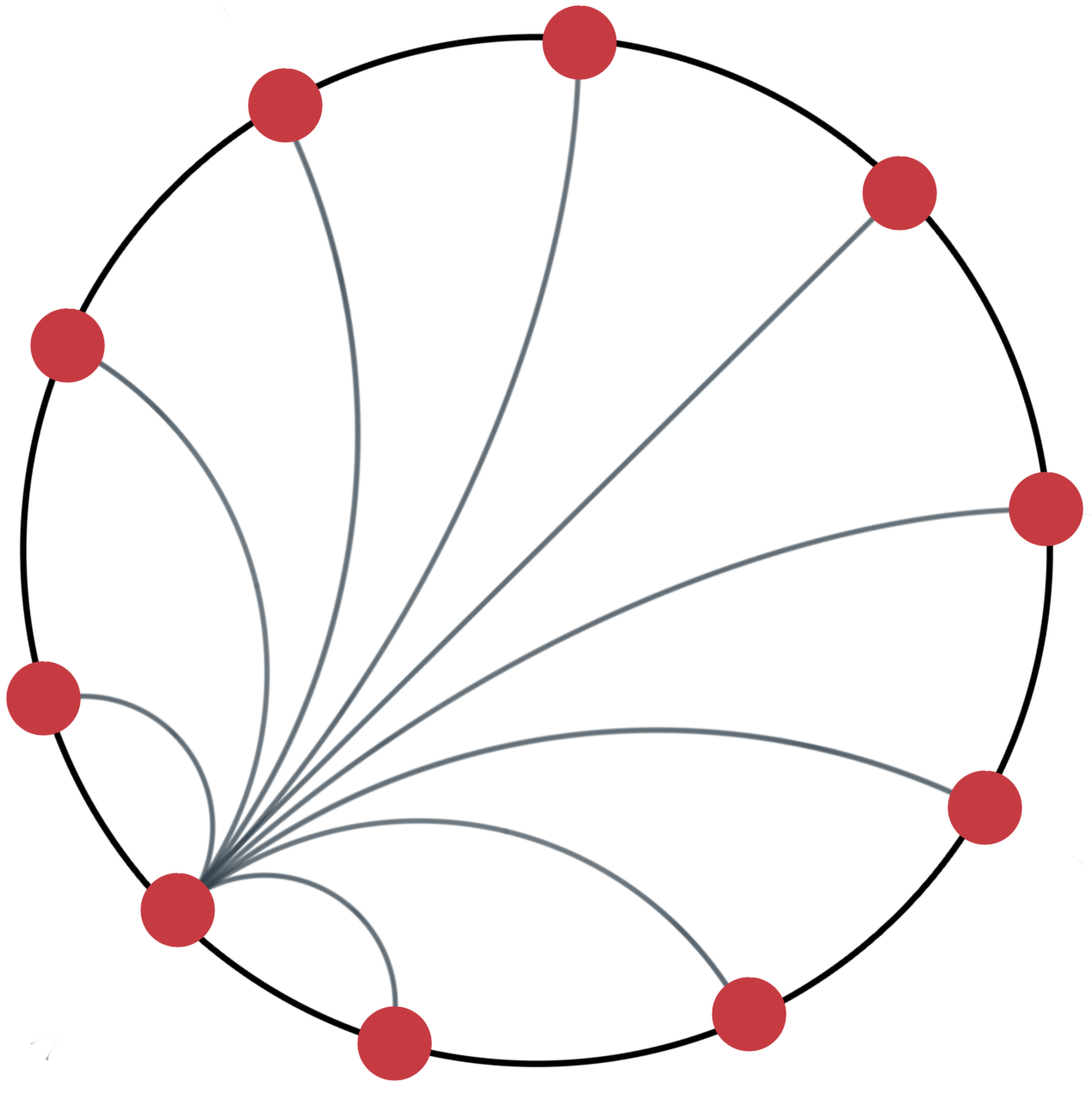
Many facts in temporal knowledge graphs induce geometric structures over time. For instance, increasing trade exchanges and economic cooperation between two major economies might promote the trade exports and economic growths of a series of countries in the downstream supply chain, which exhibits a tree-like structure over time. Moreover, an establishment of diplomatic relations between two countries might lead to regular official visits between these two countries, which produces a cyclic structure over time. Embedding methods in Euclidean space have limitations and suffer from large distortion when representing large-scale hierarchical data. Recently, hyperbolic geometry has been exploited in several works (Nickel and Kiela, 2017; Ganea et al., 2018) as an effective method for learning representations of hierarchical data, where the exponential growth of distance on the boundary of the hyperbolic space naturally allows representing hierarchical structures in a compact form. While most graph-structured data has a wide variety of inherent geometric structures, e.g. partially tree-like and partially cyclical, the above studies model the latent structures in a single geometry with a constant curvature, limiting the flexibility of the model to match the hypothetical intrinsic manifold. Thus, using a product of different constant curvature spaces (Gu et al., 2018) might be helpful to match the underlying geometries of temporal knowledge graphs and provide high-quality representations.

Existing non-Euclidean approaches for knowledge graph embeddings (Balazevic et al., 2019; Kolyvakis et al., 2019) lack the ability to capture temporal dynamics available in underlying data represented by temporal KGs. The difficulty with representing the evolution of temporal KGs in non-Euclidean spaces lies in finding a way to integrate temporal information to the geometric representations of entities. In this work, we propose the dynamic evolution of Riemannian manifold embeddings (DyERNIE), a theoretically founded approach to embed multi-relational data with dynamic relationships on a product of Riemannian manifolds with different curvatures. To capture both the stationary and dynamic characteristics of temporal KGs, we characterize the time-dependent representation of an entity as movements on manifolds. For each entity, we define an initial embedding (at $t_{0}$) on each manifold and a velocity vector residing in the tangent space of the initial embedding to generate a temporal representation at each timestamp. In particular, the initial embeddings represent the stationary structural dependencies across facts, while the velocity vectors capture the time-varying properties of entities.

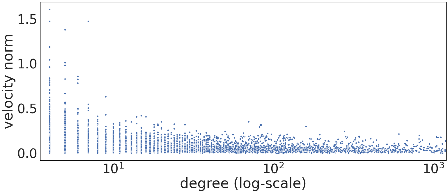
Our contributions are the following: (i) We introduce Riemannian manifolds as embedding spaces to capture geometric features of temporal KGs. (ii) We characterize the dynamics of temporal KGs as movements of entity embeddings on Riemannian manifolds guided by velocity vectors defined in the tangent space. (iii) We show how the product space can be approximately identified from sectional curvatures of temporal KGs and how to choose the dimensionality of component spaces as well as their curvatures accordingly. (iv) Our approach significantly outperforms current benchmarks on a link prediction task on temporal KGs in low- and high-dimensional settings. (v) We analyze our model’s properties, i.e. the influence of embedding dimensionality and the correlation between node degrees and the norm of velocity vectors.

2 Preliminaries

2.1 Riemannian Manifold

An $n$-dimensional Riemannian manifold $\mathcal{M}^{n}$ is a real and smooth manifold with locally Euclidean structure. For each point $\mathbf{x}\in\mathcal{M}^{n}$, the metric tensor $g(\mathbf{x})$ defines a positive-definite inner product $g(\mathbf{x})=\left\langle\cdot,\cdot\right\rangle_{\mathbf{x}}:\mathcal{T}_{\mathbf{x}}\mathcal{M}^{n}\times\mathcal{T}_{\mathbf{x}}\mathcal{M}^{n}\rightarrow\mathbb{R}$, where $\mathcal{T}_{\mathbf{x}}\mathcal{M}^{n}$ is the tangent space of $\mathcal{M}^{n}$ at $\mathbf{x}$. From the tangent space $\mathcal{T}_{\mathbf{x}}\mathcal{M}^{n}$, there exists a mapping function $\exp_{\mathbf{x}}(\mathbf{v}):\mathcal{T}_{\mathbf{x}}\mathcal{M}^{n}\rightarrow\mathcal{M}^{n}$ that maps a tangent vector $\mathbf{v}$ at $\mathbf{x}$ to the manifold, also known as the exponential map. The inverse of an exponential map is referred to as the logarithm map $\log_{\mathbf{x}}(\cdot)$.

2.2 Constant Curvature Spaces

The sectional curvature $K(\tau_{\mathbf{x}})$ is a fine-grained notion defined over a two-dimensional subspace $\tau_{\mathbf{x}}$ in the tangent space at the point $\mathbf{x}$ (Berger, 2012). If all the sectional curvatures in a manifold $\mathcal{M}^{n}$ are equal, the manifold then defined as a space with a constant curvature $K$. Three different types of constant curvature spaces can be defined depending on the sign of the curvature: a positively curved space, a flat space, and a negatively curved space. There are different models for each constant curvature space. To unify different models, in this work, we choose the stereographically projected hypersphere $\mathbb{S}^{n}_{K}$ for positive curvatures ($K>0$), while for negative curvatures ($K<0$) we choose the Poincaré ball $\mathbb{P}^{n}_{K}$, which is the stereographic projection of the hyperboloid model:

$$\mathcal{M}^{n}_{K}=\left\{\begin{aligned} \mathbb{S}^{n}_{K}&=\{\mathbf{x}\in\mathbb{R}^{n}:\left\langle\mathbf{x},\mathbf{x}\right\rangle_{2}>-1/K\}\\ \mathbb{E}^{n}&=\mathbb{R}^{n},\;\text{if}\,K=0\\ \mathbb{P}^{n}_{K}&=\{\mathbf{x}\in\mathbb{R}^{n}:\left\langle\mathbf{x},\mathbf{x}\right\rangle_{2}<-1/K\}\end{aligned}\right.$$

Both of the above spaces $\mathbb{S}_{K}$ and $\mathbb{P}_{K}$ are equipped with the Riemannian metric: $g^{\mathbb{S}_{K}}_{\mathbf{x}}=g^{\mathbb{P}_{K}}_{\mathbf{x}}=(\lambda^{K}_{\mathbf{x}})^{2}g^{\mathbb{E}}$, which is conformal to the Euclidean metric $g^{\mathbb{E}}$ with the conformal factor $\lambda^{K}_{\mathbf{x}}=2/(1+K||\mathbf{x}||^{2}_{2})$ (Ganea et al., 2018). As explained in (Skopek et al., 2019), $\mathbb{S}_{K}$ and $\mathbb{P}_{K}$ have a suitable property, namely the distance and the metric tensors of these spaces converge to their Euclidean counterpart as the curvature goes to $0$, which makes both spaces suitable for learning sign-agnostic curvatures.

2.3 Gyrovector Spaces

An important analogy to vector spaces (vector addition and scalar multiplication) in non-Euclidean geometry is the notion of gyrovector spaces (Ungar, 2008). Both the projected hypersphere and the Poincaré ball share the following definition of Möbius addition:

$$\mathbf{x}\oplus_{K}\mathbf{y}=$$

$$\frac{(1-2K\left\langle\mathbf{x},\mathbf{y}\right\rangle_{2}-K||\mathbf{y}||^{2}_{2})\mathbf{x}+(1+K||\mathbf{x}||^{2}_{2})\mathbf{y}}{1-2K\left\langle\mathbf{x},\mathbf{y}\right\rangle_{2}+K^{2}||\mathbf{x}||_{2}^{2}||\mathbf{y}||_{2}^{2}}$$

where we denote the Euclidean norm and inner product by $||\cdot||$ and $\left\langle\cdot,\cdot\right\rangle_{2}$, respectively. Skopek et al. (2019) show that the distance between two points in $\mathbb{S}_{K}$ or $\mathbb{P}_{K}$ is equivalent to their variants in gyrovector spaces, which is defined as

$$d_{\mathcal{M}_{K}}(\mathbf{x},\mathbf{y})=\frac{2}{\sqrt{|K|}}\tan_{K}^{-1}(\sqrt{|K|}||-\mathbf{x}\oplus_{K}\mathbf{y}||_{2}),$$

where $\tan_{K}=\tan$ if $K>0$ and $\tan_{K}=\tanh$ if $K<0$. The same gyrovector spaces can be used to define the exponential and logarithmic maps in the Poincaré ball and the projected hypersphere. We list these mapping functions in Table 8 in the appendix. As Ganea et al. (2018) use the exponential and logarithmic maps to obtain the Möbius matrix-vector multiplication: $\mathbf{M}\otimes_{K}\mathbf{x}=\exp^{K}_{\mathbf{0}}(\mathbf{M}\log^{K}_{\mathbf{0}}(\mathbf{x}))$, we reuse them in hyperbolic space. This operation is defined similarly in projected hyperspherical space.

2.4 Product Manifold

We further generalize the embedding space of latent representations from a single manifold to a product of Riemannian manifolds with constant curvatures. Consider a sequence of Riemannian manifolds with constant curvatures, the product manifold is defined as the Cartesian product of $k$ component manifolds $\mathcal{M}^{n}=\boldsymbol{\bigtimes}_{i=1}^{k}\mathcal{M}_{K_{i}}^{n_{i}}$, where $n_{i}$ is the dimensionality of the $i-$th component, and $K_{i}$ indicates its curvature, with choices $\mathcal{M}_{K_{i}}^{n_{i}}\in\{\mathbb{P}_{K_{i}}^{n_{i}},\mathbb{E}^{n_{i}},\mathbb{S}_{K_{i}}^{n_{i}}\}$. We call $\{(n_{i},k_{i})\}_{i=1}^{k}$ the signature of a product manifold. Note that the notation $\mathbb{E}^{n_{i}}$ is redundant in Euclidean spaces since the Cartesian product of Euclidean spaces with different dimensions can be combined into a single space, i.e. $\mathbb{E}^{n}=\bigtimes^{k}_{i=1}\mathbb{E}^{n_{i}}$. However, this equality does not hold in the projected hypersphere and the Poincaré ball. For each point $\mathbf{x}\in\mathcal{M}^{n}$ on a product manifold, we decompose its coordinates into the corresponding coordinates in component manifolds $\mathbf{x}=(\mathbf{x}^{(1)},...,\mathbf{x}^{(k)})$, where $\mathbf{x}^{(i)}\in\mathcal{M}_{K_{i}}^{n_{i}}$. The distance function decomposes based on its definition $d_{\mathcal{M}^{n}}^{2}(\mathbf{x},\mathbf{y})=\sum_{i=1}^{k}d_{\mathcal{M}^{n_{i}}_{K_{i}}}^{2}(\mathbf{x}^{(i)},\mathbf{y}^{(i)})$. Similarly, we decompose the metric tensor, exponential and logarithmic maps on a product manifold into the component manifolds. In particular, we split the embedding vectors into parts $\mathbf{x}^{(i)}$, apply the desired operation on that part $f^{n_{i}}_{K_{i}}(\mathbf{x}^{(i)})$, and concatenate the resulting parts back (Skopek et al., 2019).

2.5 Temporal Knowledge Graph Completion

Temporal knowledge graphs (KGs) are multi-relational, directed graphs with labeled timestamped edges between entities. Let $\mathcal{E}$, $\mathcal{P}$, and $\mathcal{T}$ represent a finite set of entities, predicates, and timestamps, respectively. Each fact can be denoted by a quadruple $q=(e_{s},p,e_{o},t)$, where $p\in\mathcal{P}$ represents a timestamped and labeled edge between a subject entity $e_{s}\in\mathcal{E}$ and an object entity $e_{o}\in\mathcal{E}$ at a timestamp $t\in\mathcal{T}$. Let $\mathcal{F}$ represents the set of all quadruples that are facts, i.e. real events in the world, the temporal knowledge graph completion (tKGC) is the problem of inferring $\mathcal{F}$ based on a set of observed facts $\mathcal{O}$, which is a subset of $\mathcal{F}$. To evaluate the proposed algorithms, the task of tKGC is to predict either a missing subject entity $(?,p,e_{o},t)$ given the other three components or a missing object entity $(e_{s},p,?,t)$. Taking the object prediction as an example, we consider all entities in the set $\mathcal{E}$, and learn a score function $\phi:\mathcal{E}\times\mathcal{P}\times\mathcal{E}\times\mathcal{T}\rightarrow\mathbb{R}$. Since the score function assigns a score to each quadruple, the proper object can be inferred by ranking the scores of all quadruples $\{(e_{s},p,e_{o_{i}},t),e_{o_{i}}\in\mathcal{E}\}$ that are accompanied with candidate entities.

3 Related work

3.1 Knowledge Graph Embedding

Static KG Embedding

Embedding approaches for static KGs can generally be categorized into bilinear models and translational models. The bilinear approaches are equipped with a bilinear score function that represents predicates as linear transformations acting on entity embeddings (Nickel et al., 2011; Trouillon et al., 2016; Yang et al., 2014; Ma et al., 2018a). Translational approaches measure the plausibility of a triple as the distance between the translated subject and object entity embeddings, including TransE (Bordes et al., 2013) and its variations (Sun et al., 2019; Kazemi and Poole, 2018). Additionally, several models are based on deep learning approaches (Nguyen et al., 2017; Dettmers et al., 2018; Schlichtkrull et al., 2018; Nathani et al., 2019; Hildebrandt et al., 2020) that apply (graph) convolutional layers on top of embeddings and design a score function as the last layer of the neural network.

Temporal KG Embedding

Recently, there have been some attempts of incorporating time information in temporal KGs to improve the performance of link prediction. Ma et al. (2018b) developed extensions of static knowledge graph models by adding a timestamp embedding to the score functions. Also, Leblay and Chekol (2018) proposed TTransE by incorporating time representations into the score function of TransE in different ways. HyTE (Dasgupta et al., 2018) embeds time information in the entity-relation space by arranging a temporal hyperplane to each timestamp. Inspired by the canonical decomposition of tensors, Lacroix et al. (2020) proposed an extension of ComplEx (Trouillon et al., 2016) for temporal KG completion by decomposing a 4-way tensor. The number of parameters of these models scales with the number of timestamps, leading to overfitting when the number of timestamps is extremely large. Additionally, a considerable amount of models (Trivedi et al., 2017; Jin et al., 2019; Han et al., 2020) have been developed for forecasting on temporal knowledge graphs, which predict future links only based on past events.

3.2 Graph Embedding Approaches in non-Euclidean Geometries

There has been a growing interest in embedding graph data in non-Euclidean spaces. Nickel and Kiela (2017) first applied hyperbolic embedding for link prediction to the lexical database WordNet. Since then, hyperbolic analogs of several other approaches have been developed (De Sa et al., 2018; Tifrea et al., 2018). In particular, Balazevic et al. (2019) proposed a translational model for embedding multi-relational graph data in the hyperbolic space and demonstrated advancements over state-over-the-art. More recently, Gu et al. (2018) generalized manifolds of constant curvature to a product manifold combining hyperbolic, spherical, and Euclidean components. However, these methods consider graph data as static models and lack the ability to capture temporally evolving dynamics.

4 Temporal Knowledge Graph Completion in Riemannian Manifold

Entities in a temporal KG might form different geometric structures under different relations, and these structures could evolve with time. To capture heterogeneous and time-dependent structures, we propose the DyERNIE model to embed entities of temporal knowledge graphs on a product of Riemannian manifolds and model time-dependent behavior of entities with dynamic entity representations.

4.1 Entity Representation

In temporal knowledge graphs, entities might have some features that change over time and some features that remain fixed. Thus, we represent the embedding of an entity $e_{j}\in\mathcal{E}$ at instance $t$ with a combination of low-dimensional vectors $\mathbf{e}_{j}(t)=(\mathbf{e}_{j}^{(1)}(t),...,\mathbf{e}_{j}^{(k)}(t))$ with $\mathbf{e}_{j}^{(i)}(t)\in\mathcal{M}^{n_{i}}_{K_{i}}$, where $\mathcal{M}^{n_{i}}_{K_{i}}\in\{\mathbb{P}_{K_{i}}^{n_{i}},\mathbb{E}^{n_{i}},\mathbb{S}_{K_{i}}^{n_{i}}\}$ is the $i$-th component manifold, $K_{i}$ and $n_{i}$ denote the curvature and the dimension of this manifold, respectively. Each component embedding $\mathbf{e}_{j}^{(i)}(t)$ is derived from an initial embedding and a velocity vector to encode both the stationary properties of the entities and their time-varying behavior, namely

$$\mathbf{e}_{j}^{(i)}(t)=\exp^{K_{i}}_{\mathbf{0}}\left(\log^{K_{i}}_{\mathbf{0}}(\mathbf{\bar{e}}_{j}^{(i)})+\mathbf{v}_{e_{j}^{(i)}}t\right),$$ (1)

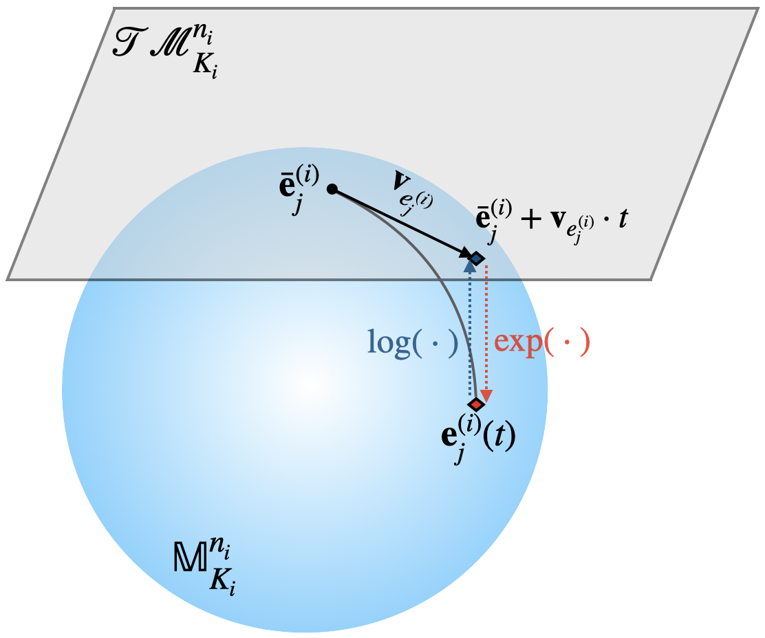
where $\mathbf{\bar{e}}_{j}^{(i)}\in\mathcal{M}^{n_{i}}_{K_{i}}$ represents the initial embedding that does not change over time. $\mathbf{v}_{e_{j}^{(i)}}\in\mathcal{T}_{\mathbf{0}}{\mathcal{M}^{n_{i}}_{K_{i}}}$ represents an entity-specific velocity vector that is defined in the tangent space at origin $\mathbf{0}$ and captures evolutionary dynamics of the entity $e_{j}$ in its vector space representations over time. As shown in Figure 1 (a), we project the initial embedding to the tangent space $\mathcal{T}_{\mathbf{0}}{\mathcal{M}^{n_{i}}_{K_{i}}}$ using the logarithmic map $\log^{K_{i}}_{\mathbf{0}}$ and then use a velocity vector to obtain the embedding of the next timestamp. Finally, we project it back to the manifold with the exponential map $\exp^{K_{i}}_{\mathbf{0}}$. Note that in the case of Euclidean space, the exponential map and the logarithmic map are equal to the identity function. By learning both the initial embedding and velocity vector, our model characterizes evolutionary dynamics of entities as movements on manifolds and thus predict unseen entity interactions based on both the stationary and time-varying entity properties.

Figure 1: (a) Evolution of an entity embedding on the $i$-th component manifold (left). For convenience in drawing, the tangent space $\mathcal{T}\mathcal{M}^{n_{i}}_{K_{i}}$ is defined at $\mathbf{\bar{e}}_{j}^{(i)}$. (b) Geodesics in the Poincaré disk (right), where red dots represent nodes on the disk.

4.2 Score Function

Bilinear models have been proved to be an effective approach for KG completion (Nickel et al., 2011; Lacroix et al., 2018), where the score function is a bilinear product between subject entity, predicate, and object entity embeddings. However, there is no clear correspondence of the Euclidean inner-product in non-Euclidean spaces. We follow the method suggested in Poincaré Glove (Tifrea et al., 2018) to reformulate the inner product as a function of distance, i.e. $\left\langle\mathbf{x},\mathbf{y}\right\rangle=\frac{1}{2}(d(\mathbf{x},\mathbf{y})^{2}+||x||^{2}+||y||^{2})$ and replace squared norms with biases $b_{\mathbf{x}}$ and $b_{\mathbf{y}}$. In addition, to capture different hierarchical structures under different relations simultaneously, Balazevic et al. (2019) applied relation-specific transformations to entities, i.e. a stretch by a diagonal predicate matrix $\mathbf{P}\in\mathbb{R}^{n\times n}$ to subject entities and a translation by a vector offset $\mathbf{p}\in\mathbb{P}^{n}$ to object entities.

Inspired by these two ideas, we define the score function of DyERNIE as

$$\phi(e_{s},p,e_{o},t)=\sum_{i=1}^{k}-d_{\mathcal{M}^{n_{i}}_{K_{i}}}\Big{(}\mathbf{P}^{(i)}\otimes_{K_{i}}\mathbf{e}_{s}^{(i)}(t),$$

$$\mathbf{e}_{o}^{(i)}(t)\oplus_{K_{i}}\mathbf{p}^{(i)}\Big{)}^{2}+b_{s}^{(i)}+b_{o}^{(i)}$$

where $\mathbf{e}_{s}^{(i)}(t)$ and $\mathbf{e}_{o}^{(i)}(t)\in\mathcal{M}^{n_{i}}_{K_{i}}$ are embeddings of the subject and object entities $e_{s}$ and $e_{o}$ in the $i$-th component manifold, respectively. $\mathbf{p}^{(i)}\in\mathcal{M}^{n_{i}}_{K_{i}}$ is a translation vector of predicate $p$, and $\mathbf{P}^{(i)}\in\mathbb{R}^{n_{i}\times n_{i}}$ represents a diagonal predicate matrix defined in the tangent space at the origin. Since multi-relational data often has different structures under different predicate, we use predicate-specific transformations $\mathbf{P}$ and $\mathbf{p}$ to determine the predicate-adjusted embeddings of entities in different predicate-dependent structures, e.g. multiple hierarchies. The distance between the predicate-adjusted embeddings of $e_{s}$ and $e_{o}$ measures the relatedness between them in terms of a predicate $p$.

Figure 2: Histogram of sectional curvatures at each timestamps on ICEWS14 (left), and ICEWS05-15 (right).

4.3 Learning

The genuine quadruples in a temporal KG $\mathcal{G}$ are split into train, validation, and test sets. We add reciprocal relations for every quadruple, which is a standard data augmentation technique commonly used in literature (Balazevic et al., 2019; Goel et al., 2019), i.e. we add $(e_{o},p^{-1},e_{s},t)$ for every $(e_{s},p,e_{o},t)$. Besides, for each fact $(e_{s},p,e_{o},t)$ in the training set, we generate $n$ negative samples by corrupting either the object $(e_{s},p,e_{o}^{\prime},t)$ or the subject $(e_{o},p^{-1},e_{s}^{\prime},t)$ with a randomly selected entity from $\mathcal{E}$. We use the binary cross-entropy as the loss function, which is defined as

$$\mathcal{L}=$$

$$\frac{-1}{N}\sum_{m=1}^{N}\left(y_{m}\log(p_{m})+(1-y_{m})\log(1-p_{m})\right),$$

where $N$ is the number of training samples, $y_{m}$ represents the binary label indicating whether a quadruple $q_{m}$ is genuine or not, $p_{m}$ denotes the predicted probability $\sigma(\phi(q_{m}))$, and $\sigma(\cdot)$ represents the sigmoid function. Model parameters are learned using Riemannian stochastic gradient descent (RSGD) (Bonnabel, 2013), where the Riemannian gradient $\nabla_{\mathcal{M}^{n}}L$ is obtained by multiplying the Euclidean gradient $\nabla_{\mathbb{E}}$ with the inverse of the Riemannian metric tensor.

4.4 Signature Estimation

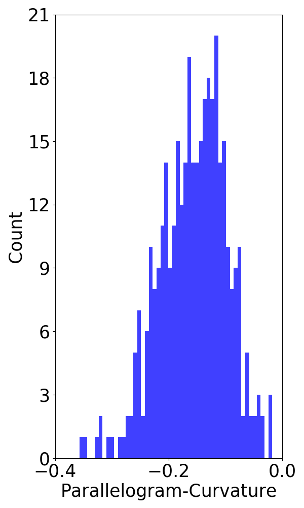
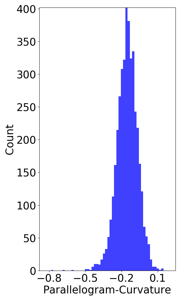
To better capture a broad range of structures in temporal KGs, we need to choose an appropriate signature of a product manifold $\mathcal{M}^{n}$, including the number of component spaces, their dimensions, and curvatures. Although we can simultaneously learn embeddings and the curvature of each component during training using gradient-based optimization, we have empirically found that treating curvature as a trainable parameter interferes with the training of other model parameters. Thus, we treat the curvature of each component and the dimension as hyperparameters selected a priori. In particular, we use the parallelogram law’ deviation (Gu et al., 2018) to estimate both the graph curvature of a given temporal KG and the number of components. Details about this algorithm can be found in Appendix A. Figure 2 shows the curvature histograms on the ICEWS14 and ICEWS05-15 datasets introduced in Section 5.1. It can be noticed that curvatures are mostly non-Euclidean, offering a good motivation to learn embeddings on a product manifold. Taking the ICEWS05-15 dataset as an example, we see that most curvatures are negative. In this case, we can initialize the product manifold consisting of three hyperbolic components with different dimensions. Then we conduct a Bayesian optimization around the initial value of the dimension and the curvature of each component to fine-tune them. Finally, we select the best-performing signature according to performance on the validation set as the final choice.

5 Experiments

5.1 Experimental Set-up

Datasets

Global Database of Events, Language, and Tone (GDELT) (Leetaru and Schrodt, 2013) dataset and Integrated Crisis Early Warning System (ICEWS) (Boschee et al., 2015) dataset have established themselves in the research community as representative samples of temporal KGs. The GDELT dataset is derived from an initiative database of all the events across the globe connecting people, organizations, and news sources. We use a subset extracted by Jin et al. (2019), which contains events occurring from 2018-01-01 to 2018-01-31. The ICEWS dataset contains information about political events with specific time annotations, e.g. (Barack Obama, visit, India, 2010-11-06). We apply our model on two subsets of the ICEWS dataset generated by García-Durán et al. (2018): ICEWS14 contains events in 2014, and ICEWS05-15 corresponds to the facts between 2005 to 2015. We compare our approach and baseline methods by performing the link prediction task on the GDELT, ICEWS14 and ICEWS05-15 datasets. The statistics of the datasets are provided in Appendix C.

Baselines

Our baselines include both static and temporal KG embedding models. From the static KG embedding models, we use TransE (Bordes et al., 2013), DistMult (Yang et al., 2014), and ComplEx (Trouillon et al., 2016) where we compress temporal knowledge graphs into a static, cumulative graph by ignoring the time information. From the temporal KG embedding models, we compare the performance of our model with several state-of-the-art methods, including TTransE (Leblay and Chekol, 2018), TDistMult/TComplEx (Ma et al., 2018b), and HyTE (Dasgupta et al., 2018).

Table 1: Link prediction results: MRR (%) and Hits@1/3/10 (%). The best results among all models are in bold. Additionally, we underline the best results among models with the same embedding dimension.

Datasets		ICEWS14 - filtered					ICEWS05-15 - filtered					GDELT - filtered
Rank ($n$)	Model	Manifold	MRR	Hits@1	Hits@3	Hits@10	Manifold	MRR	Hits@1	Hits@3	Hits@10	Manifold	MRR	Hits@1	Hits@3	Hits@10
	TransE		30.0	14.8	42.7	60.1		30.4	13.3	42.4	61.1		17.7	7.9	22.9	36.8
100	DistMult	$\mathbb{E}$	57.5	46.9	64.2	77.9	$\mathbb{E}$	47.1	33.6	55.1	72.5	$\mathbb{E}$	22.6	13.9	26.1	39.2
	ComplEx		49.3	36.6	56.2	74.2		39.0	22.9	49.2	68.4		18.8	10.5	22.2	34.9
	TTransE		34.4	25.7	38.3	51.3		35.6	15.4	51.1	67.6		18.2	0.0	30.7	46.2
	TDistMult		33.1	25.4	36.2	47.8		49.8	41.1	54.3	66.4		28.3	16.2	30.7	47.1
100	TComplEx	$\mathbb{E}$	31.8	12.9	45.7	63.0	$\mathbb{E}$	45.1	36.3	49.2	62.0	$\mathbb{E}$	30.6	21.0	34.7	48.1
	HyTE		33.1	6.8	54.5	73.6		38.1	7.6	65.0	80.4		22.4	0.0	39.5	54.2
	DyERNIE-Prod	$\mathbb{P}^{3}$	46.2	36.0	51.1	66.3	$\mathbb{P}^{3}$	58.9	50.5	63.2	75.1	$\mathbb{S}^{2}$	36.3	29.4	38.3	49.5
10	DyERNIE-Sgl	$\mathbb{P}$	43.3	33.3	47.6	62.9	$\mathbb{P}$	58.0	49.2	62.8	74.5	$\mathbb{S}$	35.7	28.7	37.7	48.9
	DyERNIE-Euclid	$\mathbb{E}$	39.8	30.6	43.6	58.2	$\mathbb{E}$	51.9	43.4	56.1	67.9	$\mathbb{E}$	30.2	23.8	31.8	42.5
	DyERNIE-Prod	$\mathbb{P}^{3}$	53.9	44.2	58.9	72.7	$\mathbb{P}^{3}$	64.2	56.5	68.2	79.0	$\mathbb{S}^{2}$	40.0	33.2	42.0	53.1
20	DyERNIE-Sgl	$\mathbb{P}$	51.3	41.4	56.1	70.3	$\mathbb{P}$	63.8	55.9	67.9	78.7	$\mathbb{S}$	39.2	32.6	41.1	52.1
	DyERNIE-Euclid	$\mathbb{E}$	47.7	38.3	52.0	66.2	$\mathbb{E}$	57.3	49.4	61.1	72.4	$\mathbb{E}$	32.9	26.2	34.7	45.7
	DyERNIE-Prod	$\mathbb{P}^{3}$	58.8	49.8	63.8	76.1	$\mathbb{P}^{3}$	68.9	61.8	72.8	82.5	$\mathbb{S}^{2}$	43.0	36.3	45.1	56.0
40	DyERNIE-Sgl	$\mathbb{P}$	56.6	47.3	61.3	74.6	$\mathbb{P}$	67.3	60.2	71.1	81.1	$\mathbb{S}$	42.5	35.8	44.6	55.6
	DyERNIE-Euclid	$\mathbb{E}$	53.7	44.2	58.6	71.9	$\mathbb{E}$	60.3	52.7	64.1	74.7	$\mathbb{E}$	38.4	31.8	40.4	51.1
	DyERNIE-Prod	$\mathbb{P}^{3}$	66.9	59.9	71.4	79.7	$\mathbb{P}^{3}$	73.9	67.9	77.3	85.5	$\mathbb{S}^{2}$	45.7	39.0	47.9	58.9
100	DyERNIE-Sgl	$\mathbb{P}$	65.7	58.2	70.2	79.4	$\mathbb{P}$	71.2	64.8	74.6	83.4	$\mathbb{S}$	45.4	38.6	47.6	58.4
	DyERNIE-Euclid	$\mathbb{E}$	63.3	54.9	67.9	79.2	$\mathbb{E}$	66.2	59.0	69.9	79.8	$\mathbb{E}$	42.6	36.1	44.5	55.1

Evaluation protocol

For each quadruple $q=(e_{s},p,e_{o},t)$ in the test set $\mathcal{G}_{test}$, we create two queries: $(e_{s},p,?,t)$ and $(e_{o},p^{-1},?,t)$. For each query, the model ranks all possible entities $\mathcal{E}$ according to their scores. Following the commonly filtered setting in the literature (Bordes et al., 2013), we remove all entity candidates that correspond to true triples from the candidate list apart from the current test entity. Let $\psi_{e_{s}}$ and $\psi_{e_{o}}$ represent the rank for $e_{s}$ and $e_{o}$ of the two queries respectively, we evaluate our models using standard metrics across the link prediction literature: mean reciprocal rank (MRR): $\frac{1}{2\cdot|\mathcal{G}_{test}|}\sum_{q\in\mathcal{G}_{test}}(\frac{1}{\psi_{e_{s}}}+\frac{1}{\psi_{e_{o}}})$ and Hits$@k(k\in\{1,3,10\})$: the percentage of times that the true entity candidate appears in the top $k$ of ranked candidates.

Implementations

We implemented our model and all baselines in PyTorch (Paszke et al., 2019). For fairness of comparison, we use Table 2 in supplementary materials to compute the embedding dimension for each (baseline, dataset) pair that matches the number of parameters of our model with an embedding dimension of $100$. Taking HyTE as an example, its embedding dimension is 193 and 151 on the ICEWS14 and GDELT dataset, respectively. Also, we use the datasets augmented with reciprocal relations to train all baseline models. We tune hyperparameters of our models using the quasi-random search followed by Bayesian optimization (Ruffinelli et al., 2020) and report the best configuration in Appendix E. We implement TTransE, TComplEx, and TDistMult based on the implementation of TransE, Distmult, and ComplEx respectively. We use the binary cross-entropy loss and RSGD to train these baselines and optimize hyperparameters by early stopping according to MRR on the validation set. Additionally, we use the implementation of HyTE. We provide the detailed settings of hyperparameters of each baseline model in Appendix B.

5.2 Comparative Study

Table 2: Filtered MRR for different choices of the distance function with $K=-1$ and $n=40$ on ICEWS14.

Distance function	MRR
$d(\mathbf{P}\otimes\mathbf{e}_{s}(t),\mathbf{e}_{o}(t)\oplus\mathbf{p})$	55.87
$\cosh(d(\mathbf{P}\otimes\mathbf{e}_{s}(t),\mathbf{e}_{o}(t)\oplus\mathbf{p}))$	54.00
$d(\mathbf{P}\otimes\mathbf{e}_{s}(t),\mathbf{P}\otimes\mathbf{e}_{o}(t))$	52.23
$d(\mathbf{P}\otimes\mathbf{e}_{s}(t),\mathbf{P}\otimes\mathbf{e}_{o}(t)\oplus\mathbf{p})$	54.55
$d(\mathbf{P}\otimes\mathbf{e}_{s}(t),\mathbf{e}_{o}(t))$	47.24
$d(\mathbf{e}_{s}(t),\mathbf{e}_{o}(t)\oplus\mathbf{p})$	51.36

Model variants

To compare the performance of non-Euclidean embeddings with their Euclidean counterparts, we implement the Euclidean version of Equation 4.2 with $d_{\mathcal{M}}(\mathbf{x},\mathbf{y})=d_{\mathbb{E}}(\mathbf{x},\mathbf{y})$. We refer to it as DyERNIE-Euclid. Besides, we train our model with a single non-Euclidean component to compare embeddings in a product space and in a manifold with a constant curvature. We refer to them as DyERNIE-Prod and DyERNIE-Sgl, respectively. For DyERNIE-Prod, we generate model configurations with different manifold combinations, i.e. $\mathbb{P}\times\mathbb{S}\times\mathbb{E},\mathbb{P}^{3}$. Details about the search space are relegated to Appendix E.

Link prediction results

We compare the baselines with three variants of our model: DyERNIE-Prod, DyERNIE-Sgl, and DyERNIE-Euclid. We report the best results on the test set among all model configurations in Table 1. Note that the number of parameters of all baselines matches our model’s with an embedding dimension of $100$. Thus, we see that both DyERNIE-Prod and DyERNIE-Sgl significantly outperform the baselines and DyERNIE-Euclid on all three datasets with the same number of parameters. Even at a low embedding dimension $(n=10)$, our models still have competitive performance, demonstrating the merits of time-dependent non-Euclidean embeddings. Besides, DyERNIE-Prod generally performs better than DyERNIE-Sgl on all three datasets. On the ICEWS14 and ICEWS05-15 datasets, we can observe that the best performing configuration of DyERNIE-Prod at each dimensionality only contains hyperbolic component manifolds. This observation confirms the curvature estimation shown in Figure 2, where most sectional curvatures on the ICEWS14 and ICEWS05-15 datasets are negative.

Table 3: Filtered MRR for different choices of entity representations with $K=-1$ and $n=40$ on ICEWS14, where $\mathbf{A}_{i}$ and $\mathbf{w}_{i}$ represent the amplitude vector and the frequency vector, respectively. $\phi_{i}$ denotes the phase shift.

Entity Representations	MRR
$\exp(\log(\mathbf{\bar{e}}_{i})+\mathbf{v}_{i}t)$	55.87
$\exp(\log(\mathbf{\bar{e}}_{i})+\mathbf{A}_{i}\sin(\mathbf{w}_{i}t+\phi_{i}))$	52.50
$\exp(\log(\mathbf{\bar{e}}_{i})+\mathbf{v}_{i}t+\mathbf{A}_{i}\sin(\mathbf{w}_{i}t+\phi_{i}))$	53.52

Ablation study

We show an ablation study of the distance function and the entity representations in Table 2 and 3, respectively. For the distance function, we use $\mathbf{p}$ and $\mathbf{P}$ to get predicate-adjusted subject and object embeddings and compute the distance between them. We found that any change to distance function causes performance degradation. Especially, removing the translation vector $\mathbf{p}$ most strongly decrease the performance. For the entity representation function, we measure the importance of a linear trend component and a non-linear periodic component. We attempt adding trigonometric functions into entity representations since a combination of trigonometric functions can capture more complicated non-linear dynamics (Rahimi and Recht, 2008). However, experimental results in Table 3 show that using only a linear transformation works the best, which indicates that finding the correct manifold of embedding space is more important than designing complicated non-linear evolution functions of entity embeddings. Additionally, we found the performance degrades significantly if removing the dynamic part of the entity embeddings. For example, on the ICEWS0515 dataset, the Hits@1 metric in the static case is only about half of that in the dynamic case, clearly showing the gain from the dynamism. Details of this ablation study are provided in Appendix G.

Figure 3: Scatter plot of distances between entity embeddings and the manifold’s origin v.s. node degrees on ICEWS05-15. Each point denotes an entity $e_{j}$. The x-coordinate gives its degree accumulated over all timestamps, and the y-coordinate represents $d_{\mathcal{M}}(\mathbf{e}_{j},\mathbf{0})$.

Figure 4: Scatter plot of velocity norms v.s. node degrees on ICEWS05-15. Each point denotes an entity.

Intrinsic hierarchical structures of temporal KGs

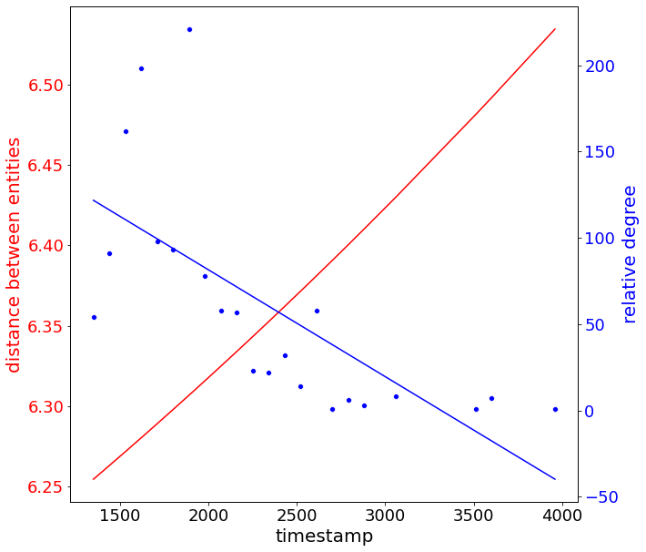
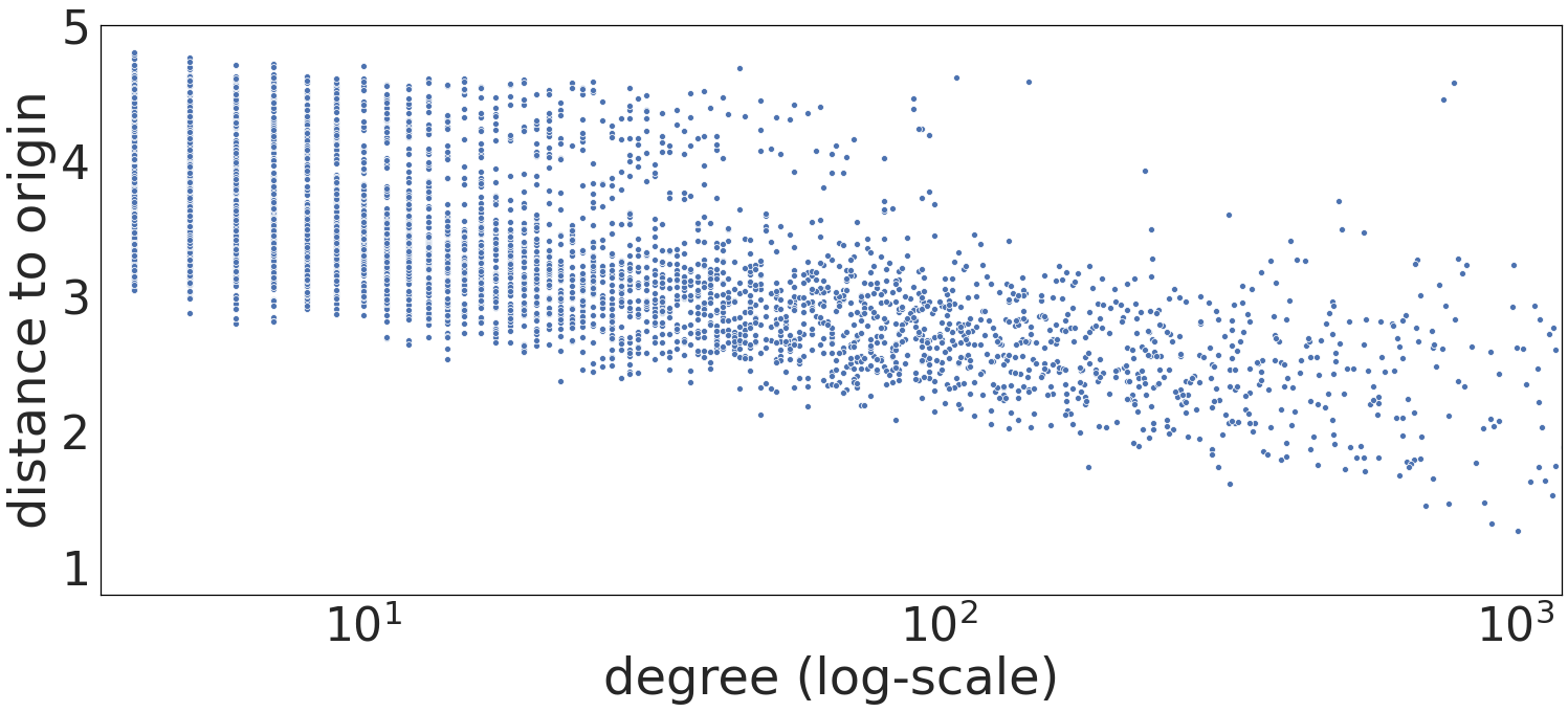
To illustrate geometric, especially the hierarchical, structures of temporal KGs, we focus on the Poincaré ball model with a dimension of $20$ and plot the geodesic distance $d_{\mathcal{M}}(\cdot,\mathbf{0})$ of learned entity embeddings to the origin of the Poincaré ball versus the degree of each entity in Figure 3. Note that the distance is averaged over all timestamps since entity embeddings are time-dependent. We observe that entities with high degrees, which means they got involved in lots of facts, are generally located close to the origin. This makes sense because these entities often lie in the top hierarchical levels. And thus, they should stand close to the root. Under the same settings, we plot the velocity norm of each entity versus the entity degree in Figure 4. Similarly, we see that entities with high degrees have a small velocity norm to stay near the origin of the manifold.

Relative movements between a node pair

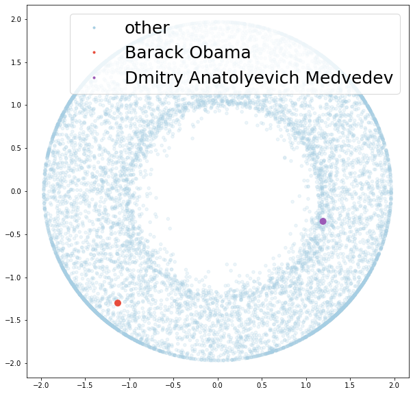
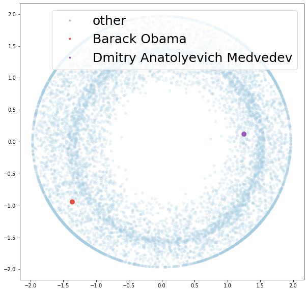
Figure 5 shows two-dimensional hyperbolic entity embeddings of the ICEWS05-15 dataset on two timestamps, 2005-01-01 and 2015-12-31. Specifically, we highlight a former US president (in orange) and a former prime minister of Russia (in purple). We found that the interaction between these two entities decreased between 2005 and 2015, as shown in Figure 9 in the appendix. Accordingly, we observe that the embeddings of these two entities were moving away from each other. More examples of learned embeddings are relegated to Appendix F.

Figure 5: Learned two-dimensional hyperbolic entity embeddings of ICEWS05-15 on the first timestamp 2005-01-01 (left) and the last timestamp 2015-12-31 (right).

6 Conclusion

In this paper, we propose an embedding approach for temporal knowledge graphs on a product of Riemannian manifolds with heterogeneous curvatures. To capture the temporal evolution of temporal KGs, we use velocity vectors defined in tangent spaces to learn time-dependent entity representations. We show that our model significantly outperforms its Euclidean counterpart and other state-of-the-art approaches on three benchmark datasets of temporal KGs, which demonstrates the significance of geometrical spaces for the temporal knowledge graph completion task.

Appendices

Appendix A Graph Curvature Estimation Algorithm

We use Algorithm 1 to estimate the sectional curvatures of a dataset developed by Bachmann et al. (2019).

Appendix B Implementation Details of Baselines

Note that the embedding dimension for each (baseline, dataset) pair matches the number of parameters of our models with an embedding dimension of $100$. We use Table 4 and 12 to compute the rank for each (baselines, dataset) pair. Besides, for fairness of results, we use the datasets augmented with reciprocal relations to train all baseline models.

Static knowledge graph embedding models

We use TransE (Bordes et al., 2013), DistMult (Yang et al., 2014), and ComplEx (Trouillon et al., 2016) as static baselines, where we compress temporal knowledge graphs into a static, cumulative graph by ignoring the time information. We use the cross-entropy loss and Adam optimizer with a batch size of 128 to train the static baselines. Besides, we use uniform sampling to initialize the embeddings of entities and predicates. Other hyperparameters of the above baselines are shown in Table 5.

Table 4: Number of parameters for each model considered when using reciprocal relations: $d$ represent the dimension of embeddings.

Model	# Parameters
ComplEx	$(2|\mathcal{E}|+4|\mathcal{P}|)\cdot d$
TransE	$(|\mathcal{E}|+2|\mathcal{P}|)\cdot d$
DistMult	$(|\mathcal{E}|+2|\mathcal{P}|)\cdot d$
TComplEx	$(2|\mathcal{E}|+4|\mathcal{P}|+2|\mathcal{T}|)\cdot d$
TTransE	$(|\mathcal{E}|+2|\mathcal{P}|+|\mathcal{T}|)\cdot d$
TDistMult	$(|\mathcal{E}|+2|\mathcal{P}|+|\mathcal{T}|)\cdot d$
HyTE	$(|\mathcal{E}|+2|\mathcal{P}|+|\mathcal{T}|)\cdot d$
DyERNIE	$2(|\mathcal{E}|+2|\mathcal{P}|)\cdot d+2|\mathcal{E}|$

Temporal knowledge graph embedding models

We compare our model’s performance with several state-of-the-art temporal knowledge graph embedding methods, including TTransE (Leblay and Chekol, 2018), TDistMult/TComplEx (Ma et al., 2018b), and HyTE (Dasgupta et al., 2018). We use the ADAM optimizer (Kingma and Ba, 2014) and the cross-entropy loss to train the temporal KG models. We set learning rate = $0.001$, negative samples pro fact = $500$, number of epochs = $500$ , batch size = $256$, and validate them every $50$ epochs to select the model giving the best validation MRR. For the GDELT dataset, we use a similar setting but with negative samples pro fact = $50$ due to the large size of the dataset. The embedding dimensions of the above dynamic baselines on each dataset are shown in Table 6.

Table 5: Hyperparameter settings of static baselines.

Model	TransE	DistMult	ComplEx
Embedding dimension
ICEWS14	202	202	101
ICEWS05-15	202	202	101
GDELT	202	202	101
Negative Sampling	253	657	1529
Learning rate	3e-4	0.16	0.18

Table 6: Embedding dimensions of dynamic baselines.

Model	TTransE	TDistMult	TComplEx	HyTE
Embedding dimension
ICEWS14	193	193	96	193
ICEWS05-15	148	148	74	148
GDELT	151	151	76	151

Appendix C Datasets

Dataset statistics are described in Table 12. Since the timestamps in the ICEWS dataset are dates rather than numbers, we sort them chronologically and encode them into consecutive numbers.

Appendix D Evaluation metrics

Let $\psi_{e_{s}}$ and $\psi_{e_{o}}$ represent the rank for $e_{s}$ and $e_{o}$ of the two queries, respectively. We evaluate our models using standard metrics across the link prediction literature: mean reciprocal rank (MRR): $\frac{1}{2\cdot|\mathcal{G}_{test}|}\sum_{q\in\mathcal{G}_{test}}(\frac{1}{\psi_{e_{s}}}+\frac{1}{\psi_{e_{o}}})$ and Hits$@k(k\in\{1,3,10\})$: the percentage of times that the true entity candidate appears in the top $k$ of ranked candidates.

Appendix E Implementation Details of DyERNIE

Signature search

On the ICEWS subsets, we try all manifold combinations with the number of components of $\{1,2,3\}$. Due to the large size of data samples on the GDELT dataset, we only try manifold combinations with the number of components of $\{1,2\}$. Specifically, the candidates are $\{\mathbb{P}^{n},\mathbb{S}^{n},\mathbb{E}^{n}\}$ for single manifolds, $\{\mathbb{P}^{n_{i}}\times\mathbb{S}^{n_{i}},\mathbb{P}^{n_{i}}\times\mathbb{P}^{n_{i}},\mathbb{S}^{n_{i}}\times\mathbb{S}^{n_{i}},\mathbb{P}^{n_{i}}\times\mathbb{E}^{n_{i}},\mathbb{S}^{n_{i}}\times\mathbb{E}^{n_{i}}\}$ for a product of two component manifolds, and $\{\mathbb{P}^{n_{i}}\times\mathbb{P}^{n_{i}}\times\mathbb{P}^{n_{i}},\mathbb{P}^{n_{i}}\times\mathbb{S}^{n_{i}}\times\mathbb{E}^{n_{i}},\mathbb{S}^{n_{i}}\times\mathbb{S}^{n_{i}}\times\mathbb{S}^{n_{i}},\mathbb{P}^{n_{i}},\times\mathbb{P}^{n_{i}}\times\mathbb{S}^{n_{i}},\mathbb{P}^{n_{i}}\times\mathbb{S}^{n_{i}}\times\mathbb{S}^{n_{i}},\mathbb{P}^{n_{i}}\times\mathbb{P}^{n_{i}}\times\mathbb{E}^{n_{i}},\mathbb{S}^{n_{i}}\times\mathbb{S}^{n_{i}}\times\mathbb{E}^{n_{i}}\}$ for a product of three component manifold. For each combination, we use the Ax-framework to optimize the assignment of dimensions to each component manifold and the curvatures. The assignment of the best-performing models are shown in Table 9, 10, and 11. We report the best results on each dataset in Table 1 in the main body.

Hyperparameter configurations for best-performing models

We select the loss function from binary cross-entropy (BCE), margin ranking loss, and cross-entropy (CE). BCE and CE give a similar performance and outperform the margin ranking loss. However, when using the BCE loss, we could use a large learning rate ($lr>10$) to speed up the training procedure. In contrast, models with the CE loss incline overfitting by large learning rates. Given the BCE loss, we found the learning rate of $50$ works the best for all model configurations. Furthermore, increasing negative samples can improve the performance to some extent, while this impact is weakening gradually as the number of negative samples become larger. However, the number of negative samples largely affect the runtime of the training procedure. We empirically found that the negative sample number of $50$ is a good compromise between the model performance and the training speed. Besides, there is no statistically significant difference in the model performance when using different optimizers, such as Riemannian Adam (RADAM) and Riemannian stochastic gradient descent (RSGD). Thus, for the model’s simplicity, we decide to use RSGD.

Average runtime for each approach $\&$ Number of parameters in each model

Table 13 shows the number of parameters and the average runtime for each model.

Appendix F Visualization

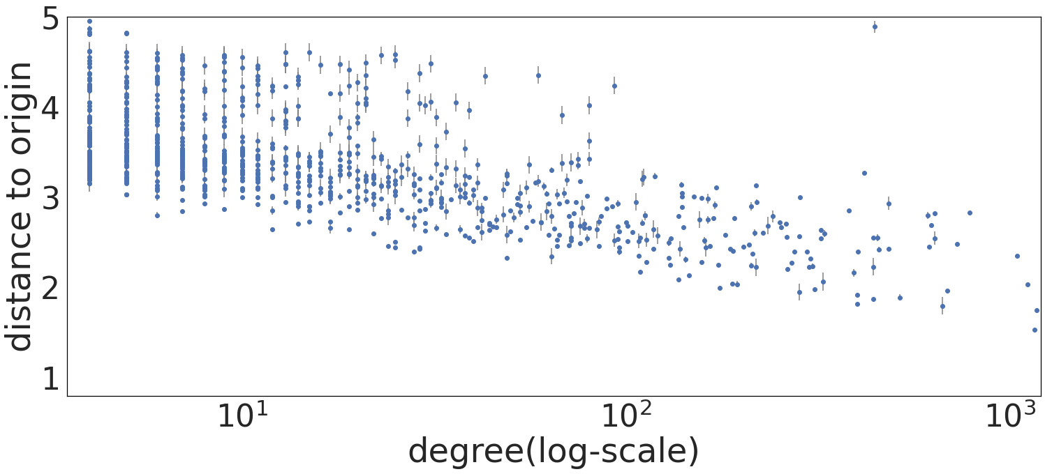
We plot the geodesic distance $d_{\mathcal{M}}(\mathbf{e}_{j},\mathbf{0})$ of learned entity embeddings with a dimension of $20$ to the manifold’s origin versus the degree of each entity in Figure 6, where $d_{\mathcal{M}}(\mathbf{e}_{j},\mathbf{0})$ is averaged over all timestamps since $\mathbf{e}_{j}$ is time-dependent. Also, the degree of each entity is accumulated over all timestamps. Each point in the upper plot represents an entity where the x-coordinate gives their degree, and the y-coordinate gives their average distance to the origin. The plot clearly shows the tendency that entities with high degrees are more likely to lie close to the origin. The bottom plot shows the same content but with a sampling of 20% points. The gray bar around each point shows the variance of the distance between the entity embedding and the origin over time.

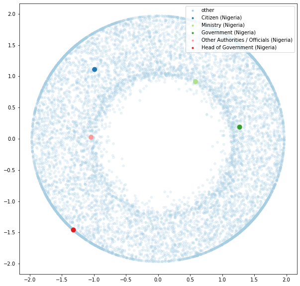
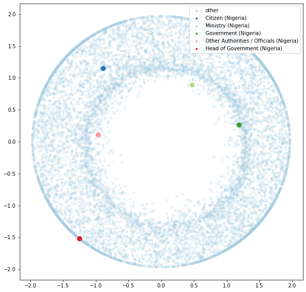
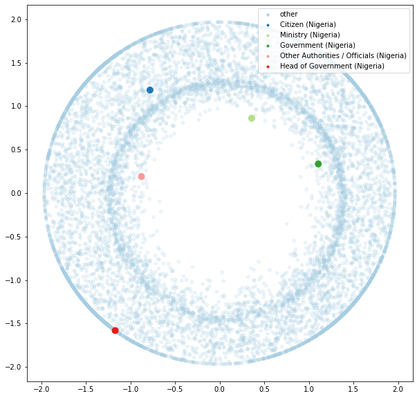
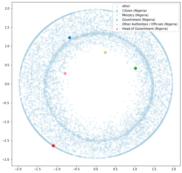
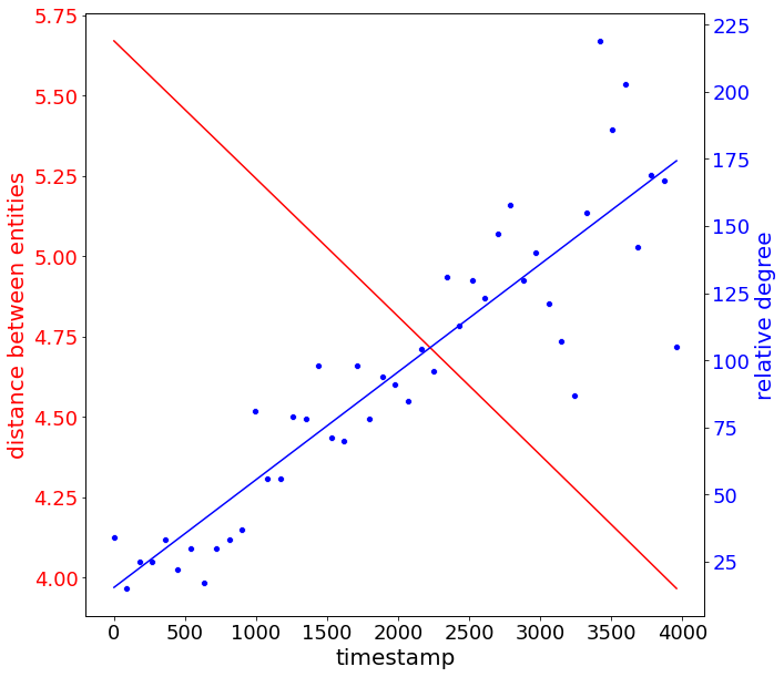
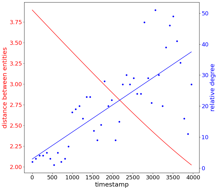
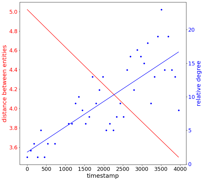
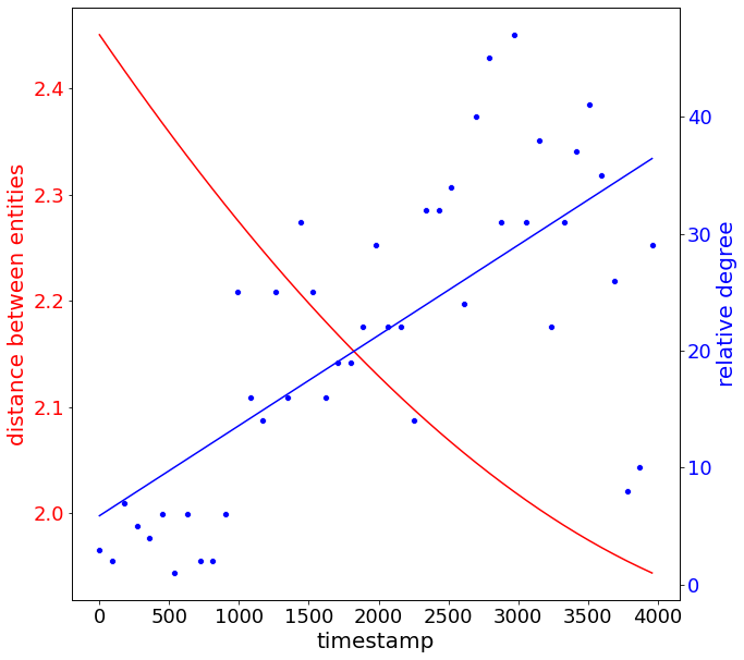
Figure 7 shows two-dimensional hyperbolic entity embeddings of the ICEWS05-15 dataset on four timestamps. We highlight some entities to show the relative movements between them. The number of interactions between the selected entities are depicted in Figure 8 and 9, which evolves over time. Specifically, we highlight Nigerian citizens, the Nigerian government, head of the Nigerian government, other authorities in Nigeria, and Nigerian minister in the first row of subplots. We can see that two entities were getting close in the Poincare disc if the number of interactions between them increases.

Appendix G Additional Ablation Study

To assess the contribution of the dynamic part of entity embeddings, we remove the dynamic part and run the model variant on static knowledge graphs. Specifically, we compress ICEWS05-15 into a static, cumulative graph by ignoring the time information. As shown in Table 7, the performance degrades significantly if the entity embeddings only have the static part. For example, on the ICEWS0515 dataset, the Hits@1 metric of DyERNIE-Sgl in the static case is less than half of that in the dynamic case, clearly showing the gain from the dynamism.

Table 7: Filtered MRR for dynamic/static entity representations with $dim=20$ on ICEWS05-15. Note that we run the static model variant on static ICEWS05-15.

Entity Representations	MRR	Hits@1	Hits@3	Hits@10
With dynamic part	63.8	55.9	67.9	78.7
Without dynamic part	38.6	28.3	42.8	59.2

Input : Number of iterations $n_{iter}$, number of timestamps $n_{time}$, Graph Slices $\{G_{i}\}_{i=1}^{n_{time}}$ of a temporal knowledge graph, Neighbor dictionary $\mathcal{N}$.

Output : $\{K_{i}\}_{i=1}^{n_{time}}$

for  $i=1$ to $n_{time}$ do

       for $m\in G_{i}$ do

             for $j=1$ to $n_{iter}$ do

                   $b,c\sim\mathcal{U}(\mathcal{N}(m))$ and $a\sim\mathcal{U}(G_{i}\backslash\{m\})$

                   $\psi_{j}(m,b,c,a)=\frac{1}{2d_{G_{i}}(a,m)}\left(2d_{G_{i}}^{2}(a,m)+d_{G_{i}}^{2}(b,c)/4-d_{G_{i}}^{2}(a,b)/2+d_{G_{i}}^{2}(a,c)/2\right)$

             end for

            $\psi_{i}(m)=\sum_{j=1}^{n_{iter}}\psi_{j}(m,b,c,a)$

       end for

      $K_{i}=\sum_{m\in G_{i}}\psi_{i}(m)$

end for

Algorithm 1 Curvature Estimation

Table 8: Exponential and logarithmic maps in Poincaré ball and projected hypersphere.

trigonometric functions	$\tan_{K}(\cdot)=\tan(\cdot)\,$ if $K>0$; $\;\tanh(\cdot)\,$ if $K<0$
Exponential map	$\exp^{K}_{\mathbf{x}}(\mathbf{v})=\mathbf{x}\oplus(\tan_{K}(\frac{\sqrt{|K|}\lambda^{K}_{\mathbf{x}}||\mathbf{v}||_{2}}{2})\frac{\mathbf{v}}{\sqrt{K}||v||_{2}})$
Logarithmic map	$\log^{K}_{\mathbf{x}}(\mathbf{v})=\frac{2}{\sqrt{|K|}\lambda^{K}_{\mathbf{x}}}\tan^{-1}_{K}(\sqrt{|K|}||-\mathbf{x}\oplus_{K}\mathbf{v}||_{2})\frac{-\mathbf{x}\oplus_{K}\mathbf{v}}{||\mathbf{x}\oplus_{K}\mathbf{v}||_{2}}$

Table 9: Hyperparameter configurations for best-performing models on the ICEWS14 dataset.

Model	DyERNIE-Sgl				DyERNIE-Prod				DyERNIE-Euclid
Embedding size	10	20	40	100	10	20	40	100	10	20	40	100
Curvature
Component A	-0.172	-0.171	-0.171	-0.170	-0.044	-0.114	-0.177	-0.346	0	0	0	0
Component B	-	-	-	-	-0.128	-0.286	-0.281	-0.137	-	-	-	-
Component C	-	-	-	-	-0.371	-0.422	-0.470	-0.855	-	-	-	-
Dimension scale
Component A	10	20	40	100	3	14	20	20	10	20	40	100
Component B	-	-	-	-	1	4	8	21	-	-	-	-
Component C	-	-	-	-	6	2	12	59	-	-	-	-

Table 10: Hyperparameter configurations for best-performing models on the ICEWS05-15 dataset.

Model	DyERNIE-Sgl				DyERNIE-Prod				DyERNIE-Euclid
Embedding size	10	20	40	100	10	20	40	100	10	20	40	100
Curvature
Component A	-0.180	-0.181	-0.179	-0.178	-0.102	-0.122	-0.298	-0.453	0	0	0	0
Component B	-	-	-	-	-0.135	-0.163	-1.243	-0.216	-	-	-	-
Component C	-	-	-	-	-0.214	-0.191	-1.819	-0.938	-	-	-	-
Dimension scale
Component A	10	20	40	100	7	10	31	32	10	20	40	100
Component B	-	-	-	-	2	8	5	52	-	-	-	-
Component C	-	-	-	-	1	2	4	16	-	-	-	-

Table 11: Hyperparameter configurations for best-performing models on the GDELT dataset.

Model	DyERNIE-Sgl				DyERNIE-Prod				DyERNIE-Euclid
Embedding size	10	20	40	100	10	20	40	100	10	20	40	100
Curvature
Component A	0.279	0.336	0.259	0.197	0.213	0.241	0.202	0.342	0	0	0	0
Component B	-	-	-	-	0.291	0.336	0.291	0.336	-	-	-	-
Dimension scale
Component A	10	20	40	100	8	8	10	68	10	20	40	100
Component B	-	-	-	-	2	12	30	32	-	-	-	-

Table 12: Datasets Statistics

Dataset Name	$|\mathcal{E}|$	$|\mathcal{P}|$	$|\mathcal{T}|$	$|\mathcal{G}|$	|$train$|	|$validation$|	|$test$|
ICEWS14	7,128	230	365	90,730	72,826	8,941	8,963
ICEWS05-15	10,488	251	4,017	479,329	386,962	46,275	46,092
GDELT	7,691	240	2,975	2,278,405	1,734,399	238,765	305,241

Table 13: Average runtime and parameter number for each approach: runtime is in seconds.

Datasets		ICEWS14			ICEWS05-15			GDELT
Rank $(d)$	Model	Manifold	Runtime	Parameters	Manifold	Runtime	Parameters	Manifold	Runtime	Parameters
	TransE		3,800	1,531,856		15,200	2,218,976		85,600	1,649,582
100	DistMult	$\mathbb{E}$	9,900	1,531,856	$\mathbb{E}$	31,500	2,218,976	$\mathbb{E}$	132,700	1,649,582
	ComplEx		4,300	1,531,856		14.100	2,218,976		76,000	1,649,582
	TTransE		55,000	1,531,856		430,000	2,218,976		1,500,000	1,649,582
	TDistMult		85,000	1,531,856		680,000	2,218,976		2,040,000	1,649,582
100	TComplEx	$\mathbb{E}$	65,000	1,531,856	$\mathbb{E}$	520,000	2,218,976	$\mathbb{E}$	1,500,000	1,649,582
	HyTE		45,000	1,531,856		360,000	2,218,976		1,100,000	1,649,582
	DyERNIE-Prod	$\mathbb{P}^{3}$	44,500	1,531,856	$\mathbb{P}^{3}$	343,800	2,218,900	$\mathbb{S}^{2}$	1,2 59,400	1,649,582
100	DyERNIE-Sgl	$\mathbb{P}$	42,000	1,531,856	$\mathbb{P}$	341,900	2,218,976	$\mathbb{S}$	1,208,300	1,649,582
	DyERNIE-Euclid	$\mathbb{E}$	19,000	1,531,856	$\mathbb{E}$	38,000	2,218,976	$\mathbb{E}$	388,800	1,649,582
	DyERNIE-Prod	$\mathbb{P}^{3}$	35,500	621,296	$\mathbb{P}^{3}$	229,500	900,176	$\mathbb{S}^{2}$	800,000	669,062
40	DyERNIE-Sgl	$\mathbb{P}$	32,000	621,296	$\mathbb{P}$	225,000	900,176	$\mathbb{S}$	740,000	669,062
	DyERNIE-Euclid	$\mathbb{E}$	11,000	621,296	$\mathbb{E}$	25,000	900,176	$\mathbb{E}$	262,000	669,062
	DyERNIE-Prod	$\mathbb{P}^{3}$	32,500	317,776	$\mathbb{P}^{3}$	225,000	460,576	$\mathbb{S}^{2}$	700,000	342,222
20	DyERNIE-Sgl	$\mathbb{P}$	31,500	317,776	$\mathbb{P}$	220,000	460,576	$\mathbb{S}$	676,000	342,222
	DyERNIE-Euclid	$\mathbb{E}$	9,500	317,776	$\mathbb{E}$	22,000	460,576	$\mathbb{E}$	240,000	342,222
	DyERNIE-Prod	$\mathbb{P}^{3}$	20,500	166,016	$\mathbb{P}^{3}$	165,000	240,776	$\mathbb{S}^{2}$	420,000	178,802
10	DyERNIE-Sgl	$\mathbb{P}$	20,500	166,016	$\mathbb{P}$	150,000	240,776	$\mathbb{S}$	400,000	178,802
	DyERNIE-Euclid	$\mathbb{E}$	6,500	166,016	$\mathbb{E}$	15,000	240,776	$\mathbb{E}$	180,000	178,802

Figure 6: Each point in the upper plot represents an entity whose x-coordinate gives their degree accumulated over all timestamps and y-coordinate gives their distance to the origin averaged over all timestamps. The plot clearly shows the tendency that entities with high degrees are more likely to lie close to the origin. The bottom plot shows the same content but with a sampling of 20% points. The gray bar around each point shows the variance of the distance over all timestamps.

Figure 7: Evolution of entity embeddings over time. We highlight Nigerian citizens, the Nigerian government, the head of Nigerian government, other authorities in Nigeria, and Nigerian minister.

(a) Citizen (Nigeria)
Government (Nigeria)

(b) Citizen (Nigeria)
Ministry (Nigeria)

(c) Government (Nigeria)
Other Authorities (Nigeria)

(d) Government (Nigeria)
Ministry (Nigeria)

Figure 8: Interaction between Nigerian entities. Subtitles show the names of the given entity pair. Red lines give the geodesic distance between two entities. Blue dots represent the number of interactions between two entities (relative degree) at each timestamp, and blue lines are regression of the relative degree between two entities over time.

Figure 9: Interaction between Barack Obama and Dmitry Anatolyevich Medvedev. Red lines give the geodesic distance between two entities. Blue dots represent the number of interactions between two entities (relative degree) at each timestamp, and blue lines are regression of the relative degree between two entities over time.

References

- Bachmann et al. (2019) Gregor Bachmann, Gary Bécigneul, and Octavian-Eugen Ganea. 2019. Constant curvature graph convolutional networks. arXiv preprint arXiv:1911.05076.
- Balazevic et al. (2019) Ivana Balazevic, Carl Allen, and Timothy Hospedales. 2019. Multi-relational poincaré graph embeddings. In Advances in Neural Information Processing Systems, pages 4465–4475.
- Berger (2012) Marcel Berger. 2012. A panoramic view of Riemannian geometry. Springer Science & Business Media.
- Bollacker et al. (2008) Kurt Bollacker, Colin Evans, Praveen Paritosh, Tim Sturge, and Jamie Taylor. 2008. Freebase: a collaboratively created graph database for structuring human knowledge. In Proceedings of the 2008 ACM SIGMOD international conference on Management of data, pages 1247–1250.
- Bonnabel (2013) Silvere Bonnabel. 2013. Stochastic gradient descent on riemannian manifolds. IEEE Transactions on Automatic Control, 58(9):2217–2229.
- Bordes et al. (2013) Antoine Bordes, Nicolas Usunier, Alberto Garcia-Duran, Jason Weston, and Oksana Yakhnenko. 2013. Translating embeddings for modeling multi-relational data. In Advances in neural information processing systems, pages 2787–2795.
- Boschee et al. (2015) Elizabeth Boschee, Jennifer Lautenschlager, Sean O’Brien, Steve Shellman, James Starz, and Michael Ward. 2015. Icews coded event data. Harvard Dataverse, 12.
- Dasgupta et al. (2018) Shib Sankar Dasgupta, Swayambhu Nath Ray, and Partha Talukdar. 2018. Hyte: Hyperplane-based temporally aware knowledge graph embedding. In Proceedings of the 2018 Conference on Empirical Methods in Natural Language Processing, pages 2001–2011.
- De Sa et al. (2018) Christopher De Sa, Albert Gu, Christopher Ré, and Frederic Sala. 2018. Representation tradeoffs for hyperbolic embeddings. Proceedings of machine learning research, 80:4460.
- Dettmers et al. (2018) Tim Dettmers, Pasquale Minervini, Pontus Stenetorp, and Sebastian Riedel. 2018. Convolutional 2d knowledge graph embeddings. In Thirty-Second AAAI Conference on Artificial Intelligence.
- Ganea et al. (2018) Octavian Ganea, Gary Bécigneul, and Thomas Hofmann. 2018. Hyperbolic neural networks. In Advances in neural information processing systems, pages 5345–5355.
- García-Durán et al. (2018) Alberto García-Durán, Sebastijan Dumančić, and Mathias Niepert. 2018. Learning sequence encoders for temporal knowledge graph completion. arXiv preprint arXiv:1809.03202.
- Goel et al. (2019) Rishab Goel, Seyed Mehran Kazemi, Marcus Brubaker, and Pascal Poupart. 2019. Diachronic embedding for temporal knowledge graph completion. arXiv preprint arXiv:1907.03143.
- Gu et al. (2018) Albert Gu, Frederic Sala, Beliz Gunel, and Christopher Ré. 2018. Learning mixed-curvature representations in product spaces.
- Han et al. (2020) Zhen Han, Yuyi Wang, Yunpu Ma, Stephan Guünnemann, and Volker Tresp. 2020. The graph hawkes network for reasoning on temporal knowledge graphs. arXiv preprint arXiv:2003.13432.
- Hildebrandt et al. (2020) Marcel Hildebrandt, Jorge Andres Quintero Serna, Yunpu Ma, Martin Ringsquandl, Mitchell Joblin, and Volker Tresp. 2020. Reasoning on knowledge graphs with debate dynamics. arXiv preprint arXiv:2001.00461.
- Hildebrandt et al. (2019) Marcel Hildebrandt, Swathi Shyam Sunder, Serghei Mogoreanu, Mitchell Joblin, Akhil Mehta, Ingo Thon, and Volker Tresp. 2019. A recommender system for complex real-world applications with nonlinear dependencies and knowledge graph context. In European Semantic Web Conference, pages 179–193. Springer.
- Jin et al. (2019) Woojeong Jin, Changlin Zhang, Pedro Szekely, and Xiang Ren. 2019. Recurrent event network for reasoning over temporal knowledge graphs. arXiv preprint arXiv:1904.05530.
- Kazemi and Poole (2018) Seyed Mehran Kazemi and David Poole. 2018. Simple embedding for link prediction in knowledge graphs. In Advances in neural information processing systems, pages 4284–4295.
- Kingma and Ba (2014) Diederik P Kingma and Jimmy Ba. 2014. Adam: A method for stochastic optimization. arXiv preprint arXiv:1412.6980.
- Kolyvakis et al. (2019) Prodromos Kolyvakis, Alexandros Kalousis, and Dimitris Kiritsis. 2019. Hyperkg: Hyperbolic knowledge graph embeddings for knowledge base completion. arXiv preprint arXiv:1908.04895.
- Lacroix et al. (2020) Timothee Lacroix, Guillaume Obozinski, and Nicolas Usunier. 2020. Tensor decompositions for temporal knowledge base completion. ICLR preprint https://openreview.net/pdf?id=rke2P1BFwS.
- Lacroix et al. (2018) Timothée Lacroix, Nicolas Usunier, and Guillaume Obozinski. 2018. Canonical tensor decomposition for knowledge base completion. arXiv preprint arXiv:1806.07297.
- Leblay and Chekol (2018) Julien Leblay and Melisachew Wudage Chekol. 2018. Deriving validity time in knowledge graph. In Companion Proceedings of the The Web Conference 2018, pages 1771–1776. International World Wide Web Conferences Steering Committee.
- Leetaru and Schrodt (2013) Kalev Leetaru and Philip A Schrodt. 2013. Gdelt: Global data on events, location, and tone, 1979–2012. In ISA annual convention, volume 2, pages 1–49. Citeseer.
- Ma et al. (2018a) Yunpu Ma, Marcel Hildebrandt, Volker Tresp, and Stephan Baier. 2018a. Holistic representations for memorization and inference. In UAI, pages 403–413.
- Ma et al. (2018b) Yunpu Ma, Volker Tresp, and Erik A Daxberger. 2018b. Embedding models for episodic knowledge graphs. Journal of Web Semantics, page 100490.
- Nathani et al. (2019) Deepak Nathani, Jatin Chauhan, Charu Sharma, and Manohar Kaul. 2019. Learning attention-based embeddings for relation prediction in knowledge graphs. arXiv preprint arXiv:1906.01195.
- Nguyen et al. (2017) Dai Quoc Nguyen, Tu Dinh Nguyen, Dat Quoc Nguyen, and Dinh Phung. 2017. A novel embedding model for knowledge base completion based on convolutional neural network. arXiv preprint arXiv:1712.02121.
- Nickel et al. (2011) Maximilian Nickel, Volker Tresp, and Hans-Peter Kriegel. 2011. A three-way model for collective learning on multi-relational data. In Icml, volume 11, pages 809–816.
- Nickel and Kiela (2017) Maximillian Nickel and Douwe Kiela. 2017. Poincaré embeddings for learning hierarchical representations. In Advances in neural information processing systems, pages 6338–6347.
- Paszke et al. (2019) Adam Paszke, Sam Gross, Francisco Massa, Adam Lerer, James Bradbury, Gregory Chanan, Trevor Killeen, Zeming Lin, Natalia Gimelshein, Luca Antiga, et al. 2019. Pytorch: An imperative style, high-performance deep learning library. In Advances in Neural Information Processing Systems, pages 8024–8035.
- Rahimi and Recht (2008) Ali Rahimi and Benjamin Recht. 2008. Random features for large-scale kernel machines. In Advances in neural information processing systems, pages 1177–1184.
- Ruffinelli et al. (2020) Daniel Ruffinelli, Samuel Broscheit, and Rainer Gemulla. 2020. You can teach an old dog new tricks! on training knowledge graph embeddings. In International Conference on Learning Representations.
- Schlichtkrull et al. (2018) Michael Schlichtkrull, Thomas N Kipf, Peter Bloem, Rianne Van Den Berg, Ivan Titov, and Max Welling. 2018. Modeling relational data with graph convolutional networks. In European Semantic Web Conference, pages 593–607. Springer.
- Skopek et al. (2019) Ondrej Skopek, Octavian-Eugen Ganea, and Gary Bécigneul. 2019. Mixed-curvature variational autoencoders. arXiv preprint arXiv:1911.08411.
- Sun et al. (2019) Zhiqing Sun, Zhi-Hong Deng, Jian-Yun Nie, and Jian Tang. 2019. Rotate: Knowledge graph embedding by relational rotation in complex space. arXiv preprint arXiv:1902.10197.
- Tifrea et al. (2018) Alexandru Tifrea, Gary Bécigneul, and Octavian-Eugen Ganea. 2018. Poincar’e glove: Hyperbolic word embeddings. arXiv preprint arXiv:1810.06546.
- Trivedi et al. (2017) Rakshit Trivedi, Hanjun Dai, Yichen Wang, and Le Song. 2017. Know-evolve: Deep temporal reasoning for dynamic knowledge graphs. In Proceedings of the 34th International Conference on Machine Learning, volume 70, pages 3462–3471. JMLR. org.
- Trouillon et al. (2016) Théo Trouillon, Johannes Welbl, Sebastian Riedel, Éric Gaussier, and Guillaume Bouchard. 2016. Complex embeddings for simple link prediction. International Conference on Machine Learning (ICML).
- Ungar (2008) Abraham Albert Ungar. 2008. A gyrovector space approach to hyperbolic geometry. Synthesis Lectures on Mathematics and Statistics, 1(1):1–194.
- Vrandečić and Krötzsch (2014) Denny Vrandečić and Markus Krötzsch. 2014. Wikidata: a free collaborative knowledgebase. Communications of the ACM, 57(10):78–85.
- Yang et al. (2014) Bishan Yang, Wen-tau Yih, Xiaodong He, Jianfeng Gao, and Li Deng. 2014. Embedding entities and relations for learning and inference in knowledge bases. arXiv preprint arXiv:1412.6575.
- Zhang et al. (2018) Yuyu Zhang, Hanjun Dai, Zornitsa Kozareva, Alexander J Smola, and Le Song. 2018. Variational reasoning for question answering with knowledge graph. In Thirty-Second AAAI Conference on Artificial Intelligence.