The School of Mathematics

Extending the statistical software package Engine for Likelihood-Free Inference
by
Vasileios Gkolemis
Dissertation Presented for the Degree of
MSc in Operational Research with Data Science
August 2020
Supervised by
Dr. Michael Gutmann

Bayesian inference is a principled framework for dealing with uncertainty. The practitioner can perform an initial assumption for the physical phenomenon they want to model (prior belief), collect some data and then adjust the initial assumption in the light of the new evidence (posterior belief). Approximate Bayesian Computation (ABC) methods, also known as likelihood-free inference techniques, are a class of models used for performing inference when the likelihood is intractable. The unique requirement of these models is a black-box sampling machine. Due to the modelling-freedom they provide these approaches are particularly captivating.

Robust Optimisation Monte Carlo (ROMC) is one of the most recent techniques of the specific domain. It approximates the posterior distribution by solving independent optimisation problems. This dissertation focuses on the implementation of the ROMC method in the software package ”Engine for Likelihood-Free Inference” (ELFI). In the first chapters, we provide the mathematical formulation and the algorithmic description of the ROMC approach. In the following chapters, we describe our implementation; (a) we present all the functionalities provided to the user and (b) we demonstrate how to perform inference on some real examples. Our implementation provides a robust and efficient solution to a practitioner who wants to perform inference on a simulator-based model. Furthermore, it exploits parallel processing for accelerating the inference wherever it is possible. Finally, it has been designed to serve extensibility; the user can easily replace specific subparts of the method without significant overhead on the development side. Therefore, it can be used by a researcher for further experimentation.

Acknowledgments

I would like to thank Michael Gutmann, who was an excellent supervisor throughout the whole period of the dissertation. His directions and insights were fundamental in the completion of this thesis. Despite the difficulties of remote communication, our collaboration remained pleasant and constructive.

Above all, a special thank to my family for supporting me all this season. Without their support, I would not have made it to complete this program.

Own Work Declaration

I declare that this thesis was composed by myself and that the work contained therein is my own, except where explicitly stated otherwise in the text.

Vasileios Gkolemis

1 Introduction

This dissertation is mainly focused on the implementation of the Robust Optimisation Monte Carlo (ROMC) method as it was proposed by [Ikonomov2019], at the Python package ELFI - ”Engine For Likelihood-Free Inference” [1708.00707]. ROMC is a novel likelihood-free inference approach for simulator-based models.

1.1 Motivation

Explanation of simulation-based models

A simulator-based model is a parameterised stochastic data generating mechanism [Gutmann2016]. The key characteristic of these models is that although we can sample (simulate) data points, we cannot evaluate the likelihood of a specific set of observations $\mathbf{y_{0}}$. Formally, a simulator-based model is described as a parameterised family of probability density functions $\{p_{\mathbf{y}|\boldsymbol{\theta}}(\mathbf{y})\}_{\boldsymbol{\theta}}$, whose closed-form is either unknown or intractable to evaluate. Whereas evaluating $p_{\mathbf{y}|\boldsymbol{\theta}}(\mathbf{y})$ is intractable, sampling is feasible. Practically, a simulator can be understood as a black-box machine $M_{r}$ that given a set of parameters $\boldsymbol{\theta}$, produces samples $\mathbf{y}$ in a stochastic manner i.e. $M_{r}(\boldsymbol{\theta})\rightarrow\mathbf{y}$.

Simulator-based models are particularly captivating due to the modelling freedom they provide; any physical process that can be conceptualised as a computer program of finite (deterministic or stochastic) steps can be modelled as a simulator-based model without any compromise. The modelling freedom includes any amount of hidden (unobserved) internal variables or logic-based decisions. As always, this degree of freedom comes at a cost; performing the inference is particularly demanding from both computational and mathematical perspective. Unfortunately, the algorithms deployed so far permit the inference only at low-dimensionality parametric spaces, i.e. $\boldsymbol{\theta}\in\mathbb{R}^{D}$ where $D$ is small.

Example

For underlying the importance of simulator-based models, let us use the tuberculosis disease spread example as described in [Tanaka2006]. An overview of the disease spread model is presented at figure 1. At each stage one of the following unobserved events may happen; (a) the transmission of a specific haplotype to a new host, (b) the mutation of an existent haplotype or (c) the exclusion of an infectious host (recovers/dies) from the population. The random process, which stops when $m$ infectious hosts are reached, can be parameterised by the transmission rate $\alpha$, the mutation rate $\tau$ and the exclusion rate $\delta$, creating a $3D$-parametric space $\boldsymbol{\theta}=(\alpha,\tau,\delta)$. The outcome of the process is a variable-size tuple $\mathbf{y}_{\boldsymbol{\theta}}$, containing the population contaminated by each different haplotype, as described in figure 1. Let’s say that the disease has been spread in a real population and when $m$ hosts were contaminated simultaneously, the vector with the infectious populations has been measured to be $\mathbf{y_{0}}$. We would like to discover the parameters $\boldsymbol{\theta}=(\alpha,\tau,\delta)$ that generated the spreading process and led to the specific outcome $\mathbf{y_{0}}$. Computing $p(\mathbf{y}=\mathbf{y_{0}}|\boldsymbol{\theta})$ requires tracking all tree-paths that could generate the specific tuple; such exhaustive enumeration becomes intractable when $m$ grows larger, as in real-case scenarios. In figure 1 we can observe that a transmission followed by a recovery/death creates a loop, reinstating the process to the previous step, which also complicates the exhaustive enumeration. Hence, representing the process with a simulator-based model and performing likelihood-free inference is the recommended solution.

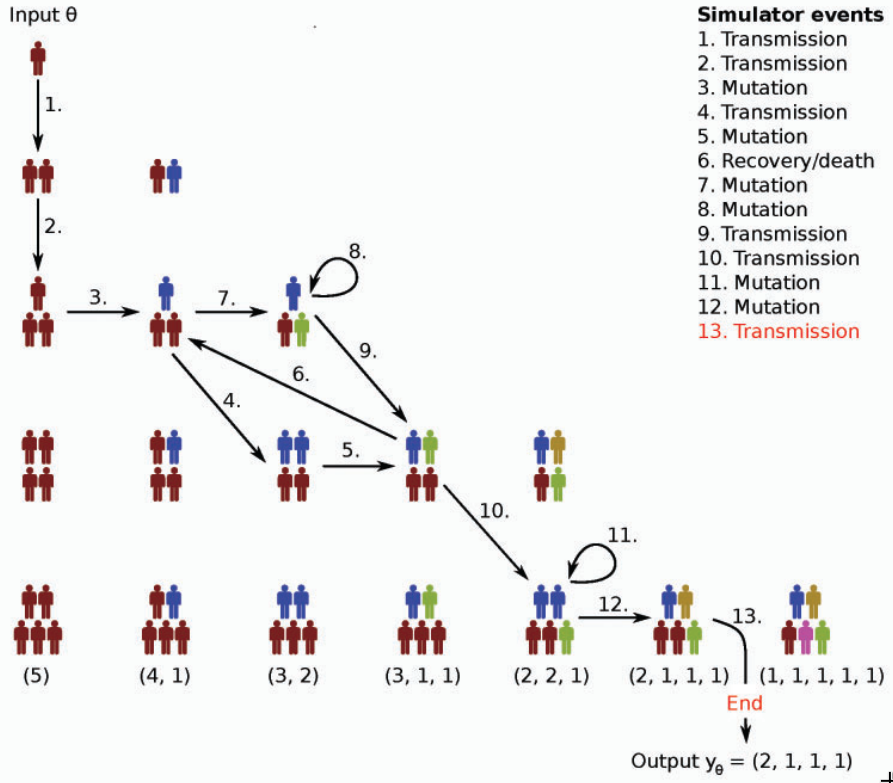
Figure 1: Depiction of a random example from the tuberculosis spreading process. The image has been taken from [Lintusaari2017].

Goal of Simulation-Based Models

As in most Machine Learning (ML) concepts, the fundamental goal is the derivation of one(many) parameter configuration(s) $\boldsymbol{\theta}^{*}$ that describe the data best i.e. generate samples $M_{r}(\boldsymbol{\theta}^{*})$ that are as close as possible to the observed data $\mathbf{y_{0}}$. In our case, following the approach of Bayesian ML, we treat the parameters of interest $\boldsymbol{\theta}$ as random variables and we try to infer a posterior distribution $p(\boldsymbol{\theta}|\mathbf{y_{0}})$ on them.

Robust Optimisation Monte Carlo (ROMC) method

The ROMC method [Ikonomov2019] is very a recent likelihood-free approach. Its fundamental idea is the transformation of the stochastic data generation process $M_{r}(\boldsymbol{\theta})$ to a deterministic mapping $g_{i}(\boldsymbol{\theta})$, by sampling the variables that produce the randomness $\mathbf{v}_{i}\sim p(\mathbf{V})$. Formally, in every stochastic process the randomness is influenced by a vector of random variables $\mathbf{V}$, whose state is unknown prior to the execution of the simulation; sampling the state makes the procedure deterministic, namely $g_{i}(\boldsymbol{\theta})=M_{d}(\boldsymbol{\theta},\mathbf{V}=\mathbf{v}_{i})$. This approach initially introduced at [Meeds2015] with the title Optimisation Monte Carlo (OMC). The ROMC extended this approach by resolving a fundamental failure-mode of OMC. The ROMC describes a methodology for approximating the posterior through a series of steps, without explicitly enforcing which algorithms must be utilised for each step; in this sense, it can be perceived as a meta-algorithm.

Implementation

The most important contribution of this work is the implementation of the ROMC method in the Python package Engine for Likelihood-Free Inference (ELFI) [1708.00707]. Since the method has been published quite recently, it has not been implemented by now in any ML software. This work attempts to provide the research community with a robust and extensible implementation for further experimentation.

1.2 Outline of Thesis

The remainder of the dissertation is organised as follows; in Chapter 2, we establish the mathematical formulation. Namely, we initially describe the simulator-based models and provide some background information on the fundamental algorithms proposed so far. Afterwards, we provide the mathematical description of the ROMC approach [Ikonomov2019]. Finally, we transform the mathematical description to algorithms. In Chapter 3, we illustrate the implementation part; we initially provide some information regarding the Python package Engine for Likelihood-Free Inference (ELFI) [1708.00707] and subsequently, we present the implementation details of ROMC in this package. In general, the conceptual scheme followed by the dissertation is

$$\text{Mathematical modelling}\rightarrow\text{Algorithm}\rightarrow\text{Software}$$

In Chapter 4, we demonstrate the functionalities of the ROMC implementation at some real-world examples; this chapter demonstrates the accuracy of the ROMC method and our implementation’s at likelihood-free tasks. Finally, in Chapter 5, we conclude with some thoughts on the work we have done and some future research ideas.

1.3 Notation

In this section, we provide an overview of the symbols utilised in the rest of the document. At this level, the quantities are introduced quite informally; most of them will be defined formally in the next chapters. We try to keep the notation as consistent as possible throughout the document. The symbol $\mathbb{R}^{N}$, when used, describes that a variable belongs to the N-dimensional Euclidean space; $N$ does not represent a specific number. The bold formation ($\mathbf{x}$) indicates a vector, while ($x$) a scalar. Random variables are represented with capital letters ($\mathbf{\Theta}$) while the samples with lowercase letters ($\boldsymbol{\theta}$), i.e. $\boldsymbol{\theta}\sim\mathbf{\Theta}$.

Random Generator

• $M_{r}(\boldsymbol{\theta}):\mathbb{R}^{D}\rightarrow\mathbb{R}$: The black-box data simulator

Parameters/Random Variables/Symbols

• $D\in\mathbb{N}$, the dimensionality of the parameter-space

• $\mathbf{\Theta}\in\mathbb{R}^{D}$, random variable representing the parameters of interest

• $\mathbf{y_{0}}\in\mathbb{R}^{N}$, the vector with the observations

• $\epsilon\in R$, the threshold setting the limit on the region around $\mathbf{y_{0}}$. When further notation is introduced regarding $\epsilon$

  • $\epsilon_{filter}$, threshold for discarding solutions

  • $\epsilon_{region}$, threshold for building bounding box regions

  • $\epsilon_{cutoff}$, threshold for the indicator function

• $\mathbf{V}\in\mathbb{R}^{N}$, random variable representing the randomness of the generator. It is also called nuisance variable, because we are not interested in inferring a posterior distribution on it.

• $\mathbf{v}_{i}\sim\mathbf{V}$, a specific sample drawn from $\mathbf{V}$

• $\mathbf{Y}_{\boldsymbol{\theta}}$, random variable describing the simulator $M_{r}(\boldsymbol{\theta})$.

• $\mathbf{y}_{i}\sim\mathbf{Y}_{\theta}$, a sample drawn from $\mathbf{Y}_{\theta}$. It can be obtained by executing the simulator $\mathbf{y}_{i}\sim M_{r}(\boldsymbol{\theta})$

Sets

• $B_{d,\epsilon}(\mathbf{y_{0}})$, the set of $\mathbf{y}$ points close to the observations, i.e. $\mathbf{y}:=\{\mathbf{y}:d(\mathbf{y},\mathbf{y_{0}})\leq\epsilon\}$

• $B_{d,\epsilon}^{i}$, the set of points defined around $\mathbf{y}_{i}$ i.e. $B_{d,\epsilon}^{i}=B_{d,\epsilon}(\mathbf{y}_{i})$

• $\mathcal{S}_{i}$, the set of parameters $\boldsymbol{\theta}$ that generate data close to the observations using the i-th deterministic generator, i.e. $\{\boldsymbol{\theta}:M_{d}(\boldsymbol{\theta},\mathbf{v}_{i})\in B_{d,\epsilon}(\mathbf{y_{0}})\}$

Generic Functions

• $p(\cdot)$, any valid pdf

• $p(\cdot|\cdot)$, any valid conditional distribution

• $p(\boldsymbol{\theta})$, the prior distribution on the parameters

• $p(\mathbf{v})$, the prior distribution on the nuisance variables

• $p(\boldsymbol{\theta}|\mathbf{y_{0}})$, the posterior distribution

• $p_{d,\epsilon}(\boldsymbol{\theta}|\mathbf{y_{0}})$, the approximate posterior distribution

• $d(\mathbf{x},\mathbf{y}):\mathbb{R}^{2N}\rightarrow\mathbb{R}$: any valid distance, the $L_{2}$ norm: $||\mathbf{x}-\mathbf{y}||_{2}$

Functions (Mappings)

• $M_{d}(\boldsymbol{\theta},\mathbf{v}):\mathbb{R}^{D}\rightarrow\mathbb{R}$, the deterministic generator; all stochastic variables that are part of the data generation process are represented by the parameter $\mathbf{v}$

• $f_{i}(\boldsymbol{\theta})=M_{d}(\boldsymbol{\theta},\mathbf{v}_{i})$, deterministic generator associated with sample $\mathbf{v}_{i}\sim p(\mathbf{v})$

• $g_{i}(\boldsymbol{\theta})=d(f_{i}(\boldsymbol{\theta}),\mathbf{y_{0}})$, distance of the generated data $f_{i}(\boldsymbol{\theta})$ from the observations

• $T(\mathbf{x}):\mathbb{R}^{D_{1}}\rightarrow\mathbb{R}^{D_{2}}$ where $D_{1}>D_{2}$, the mapping that computes the summary statistic

• $\mathbb{1}_{B_{d,\epsilon}(\mathbf{y_{0}})}(\mathbf{y})$, the indicator function; returns 1 if $d(\mathbf{y},\mathbf{y_{0}})\leq\epsilon$, else 0

• $L(\boldsymbol{\theta})$, the likelihood

• $L_{d,\epsilon}(\boldsymbol{\theta})$, the approximate likelihood

1.4 Online notebooks

Since the dissertation is mainly focused on the implementation of the ROMC, we have created some interactive notebooks supporting the main document. The reader is advised to exploit the notebooks in order to (a) review the code used for performing the inference (b) understand the functionalities of our implementation in a practical sense (c) check the validity of our claims and (c) interactively execute experiments.

The notebooks are provided in two formats:

• The first format is located in this Github repository. In order for the reader to experiment with the examples, they should clone the repository into their pc, execute the installation instructions and run the notebooks using the Jupyter package.

• The second format is the google colab notebook [Bisong2019]. Following the links below, the reader can view the notebook and make an online clone of it. Hence, without any installation overhead, they may interactivelly explore all the provided functionalities.

The notebooks provide a practical overview of the implemented functionalities and it are easy to use; in particular, the google colab version is entirely plug-and-play. Therefore, we encourage the reader of the dissertation to use them as supporting material. The following list contains the implemented examples along with their links:

• Simple 1D example

  • Google colab

  • Github repository

• Simple 2D example

  • Google colab

  • Github repository

• Moving Average example

  • Google colab

  • Github repository

• Extensibility example

  • Google colab

  • Github repository

2 Background

2.1 Simulator-based models

As already stated at Chapter 1, in simulator-based models we cannot evaluate the posterior $p(\boldsymbol{\theta}|\mathbf{y_{0}})\propto L(\boldsymbol{\theta})p(\boldsymbol{\theta})$, due to the intractability of the likelihood $L(\boldsymbol{\theta})=p(\mathbf{y_{0}}|\boldsymbol{\theta})$. The following equation allows incorporating the simulator in the place of the likelihood and forms the basis of all likelihood-free inference approaches,

$$L(\boldsymbol{\theta})=\lim_{\epsilon\to 0}c_{\epsilon}\int_{\mathbf{y}\in B_{d,\epsilon}(\mathbf{y_{0}})}p(\mathbf{y}|\boldsymbol{\theta})d\mathbf{y}=\lim_{\epsilon\to 0}c_{\epsilon}\Pr(M_{r}(\boldsymbol{\theta})\in B_{d,\epsilon}(\mathbf{y_{0}}))$$ (2.1)

where $c_{\epsilon}$ is a proportionality factor dependent on $\epsilon$, needed when $\Pr(M_{r}(\boldsymbol{\theta})\in B_{d,\epsilon}(\mathbf{y_{0}}))\rightarrow 0$, as $\epsilon\rightarrow 0$. Equation 2.1 describes that the likelihood of a specific parameter configuration $\boldsymbol{\theta}$ is proportional to the probability that the simulator will produce outputs equal to the observations, using this configuration.

2.1.1 Approximate Bayesian Computation (ABC) Rejection Sampling

ABC rejection sampling is a modified version of the traditional rejection sampling method, for cases when the evaluation of the likelihood is intractable. In the typical rejection sampling, a sample obtained from the prior $\boldsymbol{\theta}\sim p(\boldsymbol{\theta})$ gets accepted with probability $L(\boldsymbol{\theta})/\text{max}_{\boldsymbol{\theta}}L(\boldsymbol{\theta})$. Though we cannot use this approach out-of-the-box (evaluating $L(\boldsymbol{\theta})$ is impossible in our case), we can modify the method incorporating the simulator.

In the discrete case scenario where $\mathbf{Y}_{\boldsymbol{\theta}}$ can take a finite set of values, the likelihood becomes $L(\boldsymbol{\theta})=\Pr(\mathbf{Y}_{\boldsymbol{\theta}}=\mathbf{y_{0}})$ and the posterior $p(\boldsymbol{\theta}|\mathbf{y_{0}})\propto\Pr(\mathbf{Y}_{\boldsymbol{\theta}}=\mathbf{y_{0}})p(\boldsymbol{\theta})$; hence, we can sample from the prior $\boldsymbol{\theta}_{i}\sim p(\boldsymbol{\theta})$, run the simulator $\mathbf{y}_{i}=M_{r}(\boldsymbol{\theta}_{i})$ and accept $\boldsymbol{\theta}_{i}$ only if $\mathbf{y}_{i}=\mathbf{y_{0}}$.

The method above becomes less useful as the finite set of $\mathbf{Y}_{\boldsymbol{\theta}}$ values grows larger, since the probability of accepting a sample becomes smaller. In the limit where the set becomes infinite (i.e. continuous case) the probability becomes zero. In order for the method to work in this set-up, a relaxation is introduced; we relax the acceptance criterion by letting $\mathbf{y}_{i}$ lie in a larger set of points i.e. $\mathbf{y}_{i}\in B_{d,\epsilon}(\mathbf{y_{0}}),\epsilon>0$. The region can be defined as $B_{d,\epsilon}(\mathbf{y_{0}}):=\{\mathbf{y}:d(\mathbf{y},\mathbf{y_{0}})\leq\epsilon\}$ where $d(\cdot,\cdot)$ can represent any valid distance. With this modification, the maintained samples follow the approximate posterior,

$$p_{d,\epsilon}(\boldsymbol{\theta}|\mathbf{y_{0}})\propto Pr(\mathbf{y}\in B_{d,\epsilon}(\mathbf{y_{0}}))p(\boldsymbol{\theta})$$ (2.2)

This method is called Rejection ABC.

2.1.2 Summary Statistics

When $\mathbf{y}\in\mathbb{R}^{D}$ lies in a high-dimensional space, generating samples inside $B_{d,\epsilon}(\mathbf{y_{0}})$ becomes rare even when $\epsilon$ is relatively large; this is the curse of dimensionality. As a representative example lets make the following hypothesis;

• $d$ is set to be the Euclidean distance, hence $B_{d,\epsilon}(\mathbf{y_{0}}):=\{\mathbf{y}:||\mathbf{y}-\mathbf{y_{0}}||_{2}^{2}<\epsilon^{2}\}$ is a hyper-sphere with radius $\epsilon$ and volume $V_{hypersphere}=\frac{\pi^{D/2}}{\Gamma(D/2+1)}\epsilon^{D}$

• the prior $p(\boldsymbol{\theta})$ is a uniform distribution in a hyper-cube with side of length $2\epsilon$ and volume $V_{hypercube}=(2\epsilon)^{D}$

• the generative model is the identity function $\mathbf{y}=f(\boldsymbol{\theta})=\boldsymbol{\theta}$

The probability of drawing a sample inside the hypersphere equals the fraction of the volume of the hypersphere inscribed in the hypercube:

$$Pr(\mathbf{y}\in B_{d,\epsilon}(\mathbf{y_{0}}))=Pr(\boldsymbol{\theta}\in B_{d,\epsilon}(\mathbf{y_{0}}))=\frac{V_{hypersphere}}{V_{hypercube}}=\frac{\pi^{D/2}}{2^{D}\Gamma(D/2+1)}\rightarrow 0,\quad\text{as}\quad D\rightarrow\infty$$ (2.3)

We observe that the probability tends to $0$, independently of $\epsilon$; enlarging $\epsilon$ will not increase the acceptance rate. Intuitively, we can think that in high-dimensional spaces the volume of the hypercube concentrates at its corners. This generates the need for a mapping $T:\mathbb{R}^{D_{1}}\rightarrow\mathbb{R}^{D_{2}}$ where $D_{1}>D_{2}$, for squeezing the dimensionality of the output. This dimensionality-reduction step that redefines the area as $B_{d,\epsilon}(\mathbf{y_{0}}):=\{\mathbf{y}:d(T(\mathbf{y}),T(\mathbf{y_{0}}))\leq\epsilon\}$ is called summary statistic extraction, since the distance is not measured on the actual outputs, but on a summarisation (i.e. lower-dimension representation) of them.

2.1.3 Approximations introduced so far

So far, we have introduced some approximations for inferring the posterior as $p_{d,\epsilon}(\boldsymbol{\theta}|\mathbf{y_{0}})\propto Pr(\mathbf{Y}_{\boldsymbol{\theta}}\in B_{d,\epsilon}(\mathbf{y_{0}}))p(\boldsymbol{\theta})$ where $B_{d,\epsilon}(\mathbf{y_{0}}):=\{\mathbf{y}:d(T(\mathbf{y}),T(\mathbf{y_{0}}))<\epsilon\}$. These approximations introduce two different types of errors:

• $\epsilon$ is chosen to be big enough, so that enough samples are accepted. This modification leads to the approximate posterior introduced in (2.2)

• $T$ introduces some loss of information, making possible a $\mathbf{y}$ far away from $\mathbf{y_{0}}$ i.e. $\mathbf{y}:d(\mathbf{y},\mathbf{y_{0}})>\epsilon$, to enter the acceptance region after the dimensionality reduction $d(T(\mathbf{y}),T(\mathbf{y_{0}}))\leq\epsilon$

In the following sections, we will not use the summary statistics in our expressions for the notation not to clutter. One could understand it as absorbing the mapping $T(\cdot)$ inside the simulator. In any case, all the propositions that will be expressed in the following sections are valid with the use of summary statistics.

2.1.4 Optimisation Monte Carlo (OMC)

Before we define the likelihood approximation as introduced in the OMC, approach lets define the indicator function based on $B_{d,\epsilon}(\mathbf{y})$. The indicator function $\mathbb{1}_{B_{d,\epsilon}(\mathbf{y})}(\mathbf{x})$ returns 1 if $\mathbf{x}\in B_{d,\epsilon}(\mathbf{y})$ and 0 otherwise. If $d(\cdot,\cdot)$ is a formal distance, due to symmetry $\mathbb{1}_{B_{d,\epsilon}(\mathbf{y})}(\mathbf{x})=\mathbb{1}_{B_{d,\epsilon}(\mathbf{x})}(\mathbf{y})$, so the expressions can be used interchangeably.

$$\mathbb{1}_{B_{d,\epsilon}(\mathbf{y})}(\mathbf{x})=\left\{\begin{array}[]{ll}1&\mbox{if }\mathbf{x}\in B_{d,\epsilon}(\mathbf{y})\\ 0&\mbox{otherwise}\end{array}\right.$$ (2.6)

Based on equation (2.2) and the indicator function as defined above (2.6), we can approximate the likelihood as:

$$L_{d,\epsilon}(\boldsymbol{\theta})=\int_{\mathbf{y}\in B_{\epsilon}(\mathbf{y_{0}})}p(\mathbf{y}|\boldsymbol{\theta})d\mathbf{y}=\int_{\mathbf{y}\in\mathbb{R}^{D}}\mathbb{1}_{B_{d,\epsilon}(\mathbf{y_{0}})}(\mathbf{y})p(\mathbf{y}|\boldsymbol{\theta})d\mathbf{y}$$ (2.7)

$$\approx\frac{1}{N}\sum_{i}^{N}\mathbb{1}_{B_{d,\epsilon}(\mathbf{y_{0}})}(\mathbf{y}_{i}),\text{ where }\mathbf{y}_{i}\sim M_{r}(\boldsymbol{\theta})$$ (2.8)

$$\approx\frac{1}{N}\sum_{i}^{N}\mathbb{1}_{B_{d,\epsilon}(\mathbf{y_{0}})}(\mathbf{y}_{i})\text{ where }\mathbf{y}_{i}=M_{d}(\boldsymbol{\theta},\mathbf{v}_{i}),\mathbf{v}_{i}\sim p(\mathbf{v})$$ (2.9)

This approach is quite intuitive; approximating the likelihood of a specific $\boldsymbol{\theta}$ requires sampling from the data generator and count the fraction of samples that lie inside the area around the observations. Nevertheless, by using the approximation of equation (2.8) we need to draw $N$ new samples for each distinct evaluation of $L_{d,\epsilon}(\boldsymbol{\theta})$; this makes this approach quite inconvenient from a computational point-of-view. For this reason, we choose to approximate the integral as in equation (2.9); the nuisance variables are sampled once $\mathbf{v}_{i}\sim p(\mathbf{v})$ and we count the fraction of samples that lie inside the area using the deterministic simulators $M_{d}(\boldsymbol{\theta},\mathbf{v}_{i})\>\forall i$. Hence, the evaluation $L_{d,\epsilon}(\boldsymbol{\theta})$ for each different $\boldsymbol{\theta}$ does not imply drawing new samples all over again. Based on this approach, the unnormalised approximate posterior can be defined as:

$$p_{d,\epsilon}(\boldsymbol{\theta}|\mathbf{y_{0}})\propto p(\boldsymbol{\theta})\sum_{i}^{N}\mathbb{1}_{B_{d,\epsilon}(\mathbf{y_{0}})}(\mathbf{y}_{i})$$ (2.10)

Further approximations for sampling and computing expectations

The posterior approximation in (2.2) does not provide any obvious way for drawing samples. In fact, the set $\mathcal{S}_{i}=\{\boldsymbol{\theta}:M_{d}(\boldsymbol{\theta},\mathbf{v}_{i})\in B_{d,\epsilon}(\mathbf{y_{0}})\}$ can represent any arbitrary shape in the D-dimensional Euclidean space; it can be non-convex, can contain disjoint sets of $\boldsymbol{\theta}$ etc. We need some further simplification of the posterior for being able to draw samples from it.

As a side-note, weighted sampling could be performed in a straightforward fashion with importance sampling. Using the prior as the proposal distribution $\boldsymbol{\theta}_{i}\sim p(\boldsymbol{\theta})$ and we can compute the weight as $w_{i}=\frac{L_{d,\epsilon}(\boldsymbol{\theta}_{i})}{p(\boldsymbol{\theta}_{i})}$, where $L_{d,\epsilon}(\boldsymbol{\theta}_{i})$ is computed with the expression (2.7). This approach has the same drawbacks as ABC rejection sampling; when the prior is wide or the dimensionality $D$ is high, drawing a sample with non-zero weight is rare, leading to either poor Effective Sample Size (ESS) or huge execution time.

The OMC proposes a quite drastic simplification of the posterior; it squeezes all regions $\mathcal{S}_{i}$ into a single point $\boldsymbol{\theta}_{i}^{*}\in\mathcal{S}_{i}$ attaching a weight $w_{i}$ proportional to the volume of $\mathcal{S}_{i}$. For obtaining a $\boldsymbol{\theta}_{i}^{*}\in\mathcal{S}_{i}$, a gradient based optimiser is used for minimising $g_{i}(\boldsymbol{\theta})=d(\mathbf{y_{0}},f_{i}(\boldsymbol{\theta}))$ and the estimation of the volume of $\mathcal{S}_{i}$ is done using the Hessian approximation $\mathbf{H}_{i}\approx\mathbf{J}_{i}^{*T}\mathbf{J}_{i}^{*}$, where $\mathbf{J}_{i}^{*}$ is the Jacobian matrix of $g_{i}(\boldsymbol{\theta})$ at $\boldsymbol{\theta}_{i}^{*}$. Hence,

$$p(\boldsymbol{\theta}|\mathbf{y_{0}})\propto p(\boldsymbol{\theta})\sum_{i}^{N}w_{i}\delta(\boldsymbol{\theta}-\boldsymbol{\theta}_{i}^{*})$$ (2.11)

$$\boldsymbol{\theta}_{i}^{*}=\text{argmin}_{\boldsymbol{\theta}}\>g_{i}(\boldsymbol{\theta})$$ (2.12)

$$w_{i}\propto\frac{1}{\sqrt{det(\mathbf{J}_{i}^{*T}\mathbf{J}_{i}^{*})}}$$ (2.13)

The distribution (2.11) provides weighted samples automatically and an expectation can be computed easily with the following equation,

$$E_{p(\boldsymbol{\theta}|\mathbf{y_{0}})}[h(\boldsymbol{\theta})]=\frac{\sum_{i}^{N}w_{i}p(\boldsymbol{\theta}_{i}^{*})h(\boldsymbol{\theta}_{i}^{*})}{\sum_{i}^{N}w_{i}p(\boldsymbol{\theta}_{i}^{*})}$$ (2.14)

2.2 Robust Optimisation Monte Carlo (ROMC) approach

The simplifications introduced by OMC, although quite useful from a computational point-of-view, they suffer from some significant failure modes:

• The whole acceptable region $\mathcal{S}_{i}$, for each nuisance variable, shrinks to a single point $\boldsymbol{\theta}_{i}^{*}$; this simplification may add significant error when then the area $\mathcal{S}_{i}$ is relatively big.

• The weight $w_{i}$ is computed based only at the curvature at the point $\boldsymbol{\theta}_{i}^{*}$. This approach is error prone at many cases e.g. when $g_{i}$ is almost flat at $\boldsymbol{\theta}_{i}^{*}$, leading to a $\text{det}(\mathbf{J}_{i}^{*T}\mathbf{J}_{i}^{*})\rightarrow 0\Rightarrow w_{i}\rightarrow\infty$, thus dominating the posterior.

• There is no way to solve the optimisation problem $\boldsymbol{\theta}_{i}^{*}=\text{argmin}_{\boldsymbol{\theta}}\>g_{i}(\boldsymbol{\theta})$ when $g_{i}$ is not differentiable.

2.2.1 Sampling and computing expectation in ROMC

The ROMC approach resolves the aforementioned issues. Instead of collapsing the acceptance regions $\mathcal{S}_{i}$ into single points, it tries to approximate them with a bounding box.. A uniform distribution is then defined on the bounding box area, used as the proposal distribution for importance sampling. If we define as $q_{i}$, the uniform distribution defined on the $i-th$ bounding box, weighted sampling is performed as:

$$\boldsymbol{\theta}_{ij}\sim q_{i}$$ (2.15)

$$w_{ij}=\frac{\mathbb{1}_{B_{d,\epsilon}(\mathbf{y_{0}})}(M_{d}(\boldsymbol{\theta}_{ij},\mathbf{v}_{i}))p(\boldsymbol{\theta}_{ij})}{q(\boldsymbol{\theta}_{ij})}$$ (2.16)

Having defined the procedure for obtaining weighted samples, any expectation $E_{p(\boldsymbol{\theta}|\mathbf{y_{0}})}[h(\boldsymbol{\theta})]$, can be approximated as,

$$E_{p(\boldsymbol{\theta}|\mathbf{y_{0}})}[h(\boldsymbol{\theta})]\approx\frac{\sum_{ij}w_{ij}h(\boldsymbol{\theta}_{ij})}{\sum_{ij}w_{ij}}$$ (2.17)

2.2.2 Construction of the proposal region

In this section we will describe mathematically the steps needed for computing the proposal distributions $q_{i}$. There will be also presented a Bayesian optimisation alternative when gradients are not available.

Define and solve deterministic optimisation problems

For each set of nuisance variables $\mathbf{v}_{i},i=\{1,2,\ldots,n_{1}\}$ a deterministic function is defined as $f_{i}(\boldsymbol{\theta})=M_{d}(\boldsymbol{\theta},\mathbf{v}_{i})$. For constructing the proposal region, we search for a point $\boldsymbol{\theta}_{*}:d(f_{i}(\boldsymbol{\theta}_{*}),\mathbf{y_{0}})<\epsilon$; this point can be obtained by solving the the following optimisation problem:

$$\!\min_{\boldsymbol{\theta}} g_{i}(\boldsymbol{\theta})=d(\mathbf{y_{0}},f_{i}(\boldsymbol{\theta}))$$ (2.18a)

subject to $$g_{i}(\boldsymbol{\theta})\leq\epsilon$$ (2.18b)

We maintain a list of the solutions $\boldsymbol{\theta}_{i}^{*}$ of the optimisation problems. If for a specific set of nuisance variables $\mathbf{v}_{i}$, there is no feasible solution we add nothing to the list. The optimisation problem can be treated as unconstrained, accepting the optimal point $\boldsymbol{\theta}_{i}^{*}=\text{argmin}_{\boldsymbol{\theta}}g_{i}(\boldsymbol{\theta})$ only if $g_{i}(\boldsymbol{\theta}_{i}^{*})<\epsilon$.

Gradient-based approach

The nature of the generative model $M_{r}(\boldsymbol{\theta})$, specifies the properties of the objective function $g_{i}$. If $g_{i}$ is continuous with smooth gradients $\nabla_{\boldsymbol{\theta}}g_{i}$ any gradient-based iterative algorithm can be used for solving 2.18a. The gradients $\nabla_{\boldsymbol{\theta}}g_{i}$ can be either provided in closed form or approximated by finite differences.

Bayesian optimisation approach

In cases where the gradients are not available, the Bayesian optimisation scheme provides an alternative choice [Shahriari2016]. With this approach, apart from obtaining an optimal $\boldsymbol{\theta}_{i}^{*}$, a surrogate model $\hat{d}_{i}$ of the distance $g_{i}$ is fitted; this approximate model can be used in the following steps for making the method more efficient. Specifically, in the construction of the proposal region and in equations (2.2), (2.15), (2.17) it could replace $g_{i}$ in the evaluation of the indicator function, providing a major speed-up.

Construction of the proposal area $q_{i}$

After obtaining a $\boldsymbol{\theta}_{i}^{*}$ such that $g_{i}(\boldsymbol{\theta}_{i}^{*})<\epsilon$, we need to construct a bounding box around it. The bounding box $\mathcal{\hat{S}}_{i}$ must contain the acceptance region around $\boldsymbol{\theta}_{i}^{*}$, i.e. $\{\boldsymbol{\theta}:g_{i}(\boldsymbol{\theta})<\epsilon$, $d(\boldsymbol{\theta},\boldsymbol{\theta}_{i}^{*})<M\}$. The second condition $d(\boldsymbol{\theta},\boldsymbol{\theta}_{i}^{*})<M$ is meant to describe that if $\mathcal{S}_{i}:=\{\boldsymbol{\theta}:g_{i}(\boldsymbol{\theta})<\epsilon\}$ contains a number of disjoint sets of $\boldsymbol{\theta}$ that respect $g_{i}(\boldsymbol{\theta})<\epsilon$, we want our bounding box to fit only the one that contains $\boldsymbol{\theta}_{i}^{*}$. We seek for a bounding box that is as tight as possible to the local acceptance region (enlarging the bounding box without a reason decreases the acceptance rate) but large enough for not discarding accepted areas.

In contrast with the OMC approach, we construct the bounding box by obtaining search directions and querying the indicator function as we move on them. The search directions $\mathbf{v}_{d}$ are computed as the eigenvectors of the curvature at $\boldsymbol{\theta}_{i}^{*}$ and a line-search method is used to obtain the limit point where $g_{i}(\boldsymbol{\theta}_{i}^{*}+\kappa\mathbf{v}_{d})\geq\epsilon$. The Algorithm 3 describes the method in-depth. After the limits are obtained along all search directions, we define bounding box and the uniform distribution $q_{i}$. This is the proposal distribution used for the importance sampling as explained in (2.15).

Fitting a local surrogate model $\hat{g}_{i}$

After the construction of the bounding box $\mathcal{\hat{S}}_{i}$, we are no longer interested in the surface outside the box. In the future steps (e.g. sampling, evaluating the posterior) we will only evaluate $g_{i}$ inside the corresponding bounding box. Hence, we could fit a local surrogate model $\hat{g}_{i}$ for representing the local area around $\theta_{i}^{*}$. Doing so, in the future steps we can exploit $\hat{g}_{i}$ for evaluating the indicator function instead of running the whole deterministic simulator.

Any ML regression model may be chosen as local surrogates. The choice should consider the properties of the local region (i.e. size, smoothness). The ROMC proposes fitting a simple quadratic model. The training set $X:\mathbb{R}^{N\times D}$ is created by sampling $N$ points from the bounding box and the labels $Y:\mathbb{R}^{N}$ are the computed by evaluating $g_{i}$. The quadratic model is fitted on the data points, for minimising the square error.

This additional step places an additional step in the training part, increasing the computational demands, but promises a major speed at the inference phase (sampling, posterior evaluation). It is frequent in ML problems, to be quite generous with the execution time at the training phase, but quite eager at the inference phase. Fitting a local surrogate model aligns with this requirement.

2.3 Algorithmic description of ROMC

In this section, we will provide the algorithmic description of the ROMC method; how to solve the optimisation problems using either the gradient-based approach or the Bayesian optimisation alternative and the construction of the bounding box. Afterwards, we will discuss the advantages and disadvantages of each choice in terms of accuracy and efficiency.

At a high-level, the ROMC method can be split into the training and the inference part.

Training part

At the training (fitting) part, the goal is the estimation of the proposal regions $q_{i}$. The tasks are (a) sampling the nuisance variables $\mathbf{v}_{i}\sim p(\mathbf{v})$ (b) defining the optimisation problems $\min_{\boldsymbol{\theta}}\>g_{i}(\boldsymbol{\theta})$ (c) obtaining $\boldsymbol{\theta}_{i}^{*}$ (d) checking whether $d_{i}^{*}\leq\epsilon$ and (e) building the bounding box for obtaining the proposal region $q_{i}$. If gradients are available, using a gradient-based method is advised for obtaining $\boldsymbol{\theta}_{i}^{*}$ much faster. Providing $\nabla_{\boldsymbol{\theta}}g_{i}$ in closed-form provides an upgrade in both accuracy and efficiency; If closed-form description is not available, approximate gradients with finite-differences requires two evaluations of $g_{i}$ for every parameter $\boldsymbol{\theta}_{d}$, which works adequately well for low-dimensional problems. When gradients are not available or $g_{i}$ is not differentiable, the Bayesian optimisation paradigm exists as an alternative solution. In this scenario, the training part becomes slower due to fitting of the surrogate model and the blind optimisation steps. Nevertheless, the subsequent task of computing the proposal region $q_{i}$ becomes faster since $\hat{d}_{i}$ can be used instead of $g_{i}$; hence we avoid to run the simulator $M_{d}(\boldsymbol{\theta},\mathbf{v}_{i})$ for each query. The algorithms 1 and 2 present the above procedure.

Inference Part

Performing the inference includes one or more of the following three tasks; (a) evaluating the unnormalised posterior $p_{d,\epsilon}(\boldsymbol{\theta}|\mathbf{y_{0}})$ (b) sampling from the posterior $\boldsymbol{\theta}_{i}\sim p_{d,\epsilon}(\boldsymbol{\theta}|\mathbf{y_{0}})$ (c) computing an expectation $E_{\boldsymbol{\theta}|\mathbf{y_{0}}}[h(\boldsymbol{\theta})]$. Computing an expectation can be done easily after weighted samples are obtained using the equation 2.17, so we will not discuss it separately.

Evaluating the unnormalised posterior requires solely the deterministic functions $g_{i}$ and the prior distribution $p(\boldsymbol{\theta})$; there is no need for solving the optimisation problems and building the proposal regions. The evaluation requires iterating over all $g_{i}$ and evaluating the distance from the observed data. In contrast, using the GP approach, the optimisation part should be performed first for fitting the surrogate models $\hat{d}_{i}(\boldsymbol{\theta})$ and evaluate the indicator function on them. This provides an important speed-up, especially when running the simulator is computationally expensive.

Sampling is performed by getting $n_{2}$ samples from each proposal distribution $q_{i}$. For each sample $\boldsymbol{\theta}_{ij}$, the indicator function is evaluated $\mathbb{1}_{B_{d,\epsilon}^{i}(\mathbf{y_{0}})}(\boldsymbol{\theta}_{ij})$ for checking if it lies inside the acceptance region. If so the corresponding weight is computed as in (2.15). As before, if a surrogate model $\hat{d}$ is available, it can be utilised for evaluating the indicator function. At the sampling task, the computational benefit of using the surrogate model is more valuable compared to the evaluation of the posterior, because the indicator function must be evaluated for a total of $n_{1}\times n_{2}$ points.

In summary, we can state that the choice of using a Bayesian optimisation approach provides a significant speed-up in the inference part with the cost of making the training part slower and a possible approximation error. It is typical in many Machine-Learning use cases, being able to provide enough time and computational resources for the training phase, but asking for efficiency in the inference part.

Algorithm 1 Training Part - Gradient-based. Requires $g_{i}(\boldsymbol{\theta}),p(\boldsymbol{\theta})$

1:for $i\leftarrow 1\textrm{ to }n$ do

2:     Obtain $\boldsymbol{\theta}_{i}^{*}$ using a Gradient Optimiser

3:     if $g_{i}(\boldsymbol{\theta}_{i}^{*})>\epsilon$ then

4:         go to 1

5:     else

6:         Approximate $\mathbf{J}_{i}^{*}=\nabla g_{i}(\theta)$ and $H_{i}\approx\mathbf{J}^{T}_{i}\mathbf{J}_{i}$

7:         Use Algorithm 3 to obtain $q_{i}$      return $q_{i},p(\theta),g_{i}(\theta)$

Algorithm 2 Training Part - Bayesian optimisation. Requires $g_{i}(\boldsymbol{\theta}),p(\boldsymbol{\theta})$

1:for $i\leftarrow 1\textrm{ to }n$ do

2:     Obtain $\boldsymbol{\theta}_{i}^{*},\hat{d}_{i}(\boldsymbol{\theta})$ using a GP approach

3:     if $g_{i}(\boldsymbol{\theta}_{i}^{*})>\epsilon$ then

4:         go to 1

5:     else

6:         Approximate $H_{i}\approx\mathbf{J}^{T}_{i}\mathbf{J}_{i}$

7:         Use Algorithm 3 to obtain $q_{i}$      return $q_{i},p(\theta),\hat{d}_{i}(\theta)$

Algorithm 3 Computation of the proposal distribution $q_{i}$; Needs, a model of distance $d$, optimal point $\boldsymbol{\theta}_{i}^{*}$, number of refinements $K$, step size $\eta$ and curvature matrix $\mathbf{H}_{i}$ ($\mathbf{J}_{i}^{T}\mathbf{J}_{i}$ or GP Hessian)

1:Compute eigenvectors $\mathbf{v}_{d}$ of $\mathbf{H}_{i}$ ($d=1,\ldots,||\boldsymbol{\theta}||)$

2:for $d\leftarrow 1\textrm{ to }||\boldsymbol{\theta}||$ do

3:     $\tilde{\boldsymbol{\theta}}\leftarrow\boldsymbol{\theta}_{i}^{*}$

4:     $k\leftarrow 0$

5:     repeat

6:         repeat

7:              $\tilde{\boldsymbol{\theta}}\leftarrow\tilde{\boldsymbol{\theta}}+\eta\ \mathbf{v}_{d}$ $\triangleright$ Large step size $\eta$.

8:         until $d(f_{i}(\tilde{\boldsymbol{\theta}}),\mathbf{y_{0}})>\epsilon$

9:         $\tilde{\boldsymbol{\theta}}\leftarrow\tilde{\boldsymbol{\theta}}-\eta\ \mathbf{v}_{d}$

10:         $\eta\leftarrow\eta/2$ $\triangleright$ More accurate region boundary

11:         $k\leftarrow k+1$

12:     until $k=K$

13:     Set final $\tilde{\boldsymbol{\theta}}$ as region end point.

14:     Repeat steps 3 - 13 for $\mathbf{v}_{d}=-\mathbf{v}_{d}$

15:Fit a rectangular box around the region end points and define $q_{i}$ as uniform distribution

Algorithm 4 Sampling. Requires a function of distance $(g_{i}(\theta)$ or $\hat{d}_{i}$ or $\hat{g}_{i}),p(\theta),q_{i}$

1:for $i\leftarrow 1\textrm{ to }n_{1}$ do

2:     for $j\leftarrow 1\textrm{ to }n_{2}$ do

3:         $\boldsymbol{\theta}_{ij}\sim q_{i}$

4:         if $g_{i}(\boldsymbol{\theta}_{ij})>\epsilon$ then

5:              Reject $\theta_{ij}$

6:         else

7:              $w_{ij}=\frac{p(\boldsymbol{\theta}_{ij})}{q(\boldsymbol{\theta}_{ij})}$

8:              Accept $\boldsymbol{\theta}_{ij}$, with weight $w_{ij}$               

2.4 Engine for Likelihood-Free Inference (ELFI) package

The Engine for Likelihood-Free Inference (ELFI) [1708.00707] is a Python package dedicated to Likelihood-Free Inference (LFI). ELFI models in a convenient manner all the fundamental components of a probabilistic model such as priors, simulators, summaries and distances. Furthermore, ELFI already supports some recently proposed likelihood-free inference methods.

2.4.1 Modelling

ELFI models the probabilistic model as a Directed Acyclic Graph (DAG); it implements this functionality based on the package fig:elfi; there are edges that connect the prior distributions to the simulator, the simulator is connected to the summary statistics that consequently are connected to the distance. The distance is the output node. Samples can be obtained from all nodes through sequential sampling. The nodes that are defined as The scipy.stats package. are automatically considered as the parameters of interest and are the only nodes that, apart from sampling, should also provide PDF evaluation. The function passed as argument in the observed.

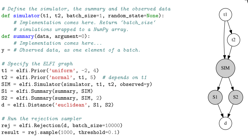
Figure 2: Baseline example for creating an model. Image taken from [1708.00707]

2.4.2 Inference Methods

The inference Methods implemented at the ELFI follow some common guidelines;

• the initial argument should is the output node of the model. It is followed by the rest hyper-parameters of the method.

• each inference method provides a central sampling functionality. In most cases it is named itemize

The collection of likelihood-free inference methods implemented so far contain the ABC Rejection Sampler, the Sequential Monte Carlo ABC Sampler and the Bayesian Optimisation for Likelihood-Free Inference (BOLFI). The latter has methodological similarities to the ROMC method that we implement in the current work.

3 Implementation

In this section, we will exhibit the implementation of the ROMC inference method in the ELFI package. The presentation is divided in two logical blocks; In section 3.1 we present our method from the user’s point-of-view, i.e. what functionalities a practitioner can use for performing the inference in a simulator-based model. For showing the functions in-practice, we set-up a simple running example and illustrate the functionalities on top of it. In section LABEL:subsec:developers we delve into the internals of the code, presenting the details of the implementation. This section mainly refers to a researcher or a developer who would like to use ROMC as a meta-algorithm and experiment with novel approaches. We have designed our implementation preserving extensibility and customisation; hence, a researcher may intervene in parts of the method without too much effort. A driver example which demonstrates how to extend the method with custom utilities is also contained in this section.

3.1 Implementation description from the user’s point-of-view

In section 3.1.1 we present an overview of the implementation. Afterwards, we divide the functionalities in 3 parts; in section 3.1.2 we present the methods used for training (fitting) the model, in section 3.1.3 those used for performing the inference and in section LABEL:subsec:evaluation those used for evaluating the approximate posterior and the obtained samples.

3.1.1 General design

In figure 4 we present an overview of our implementation; one may interpret figure 4 as a depiction of the main class of our implementation, called fig:romc_overview groups the ROMC implementation into the training, the inference and the evaluation part. The training part includes all the steps until the computation of the proposal regions; sampling the nuisance variables, defining the optimisation problems, solving them, constructing the regions and fitting local surrogate models. The inference part comprises of evaluating the unnormalised posterior (and the normalised one, in low-dimensional cases), sampling and computing an expectation. Moreover, the ROMC implementation provides some utilities for inspecting the training process, such as plotting the histogram of the distances $d^{*}_{i}=g_{i}(\theta_{i}^{*}),\>\forall i\in\{1,\ldots,n_{1}\}$ after solving the optimisation problems and visualising the constructed bounding box. Finally, two functionalities for evaluating the inference are implemented; (a) computing the Effective Sample Size (ESS) of the weighted samples and (b) measuring the divergence between the approximate posterior the ground-truth, if the latter is available.

Parallelising the processes

As stated above, the most critical advantage of the ROMC method is that it can be fully parallelised. In our implementation, we have exploited this fact by implementing a parallel version in the following tasks; (a) solving the optimisation problems, (b) constructing bounding box regions, (c) sampling and (d) evaluating the posterior. Parallelism has been achieved using the package Pool

object, which offers a convenient means of parallelising the execution of a function across multiple input values (data parallelism). For activating the parallel version of the algorithms, the user has to just pass the argument ROMC method.

Simple one-dimensional example

For illustrating the functionalities we choose as running example the following model, introduced by [Ikonomov2019],

$$p(\theta)=\mathcal{U}(\theta;-2.5,2.5)$$ (3.1)

$$p(y|\theta)=\left\{\begin{array}[]{ll}\theta^{4}+u&\mbox{if }\theta\in[-0.5,0.5]\\ |\theta|-c+u&\mbox{otherwise}\end{array}\right.$$ (3.4)

$$u\sim\mathcal{N}(0,1)$$ (3.5)

In the model (3.1), the prior is the uniform distribution in the range $[-2.5,2.5]$ and the likelihood a Gaussian distribution. There is only one observation $y_{0}=0$. The inference in this particular example can be performed quite easily, without incorporating a likelihood-free inference approach. We can exploit this fact for validating the accuracy of our implementation. The ground-truth posterior, approximated computationally, is shown in figure 3.

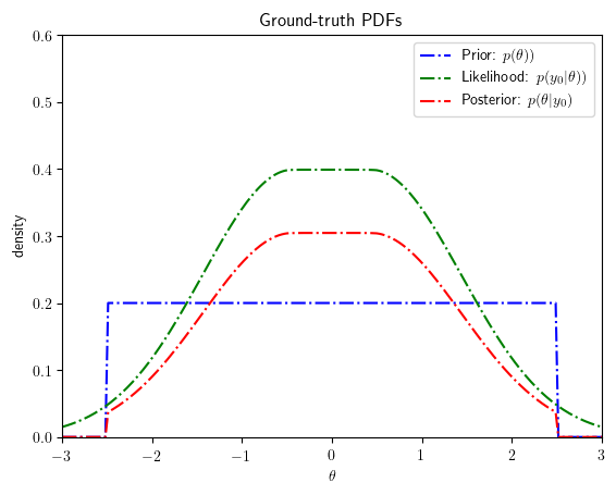
Figure 3: Ground-truth posterior distribution of the simple 1D example.

ELFI code for modelling the example

In the following code snippet, we code the model at ELFI and we initialise the ROMC inference method. We observe that the initialisation of the ROMC inference method is quite intuitive; we just pass the final (distance) node of the simulator as argument, as in all ELFI inference methods. The argument pythoncode import elfi import scipy.stats as ss import numpy as np def simulator(t1, batch_size=1,random_state=None): if t1 ¡ -0.5: y = ss.norm(loc=-t1-c, scale=1).rvs(random_state=random_state) elif t1 ¡= 0.5: y = ss.norm(loc=t1**4, scale=1).rvs(random_state=random_state) else: y = ss.norm(loc=t1-c, scale=1).rvs(random_state=random_state) return y # observation y = 0 # Elfi graph t1 = elfi.Prior(’uniform’, -2.5, 5) sim = elfi.Simulator(simulator, t1, observed=y) d = elfi.Distance(’euclidean’, sim) # Initialise the ROMC inference method bounds = [(-2.5, 2.5)] # limits of the prior parallelize = True # activate parallel execution romc = elfi.ROMC(d, bounds=bounds, parallelize=parallelize)

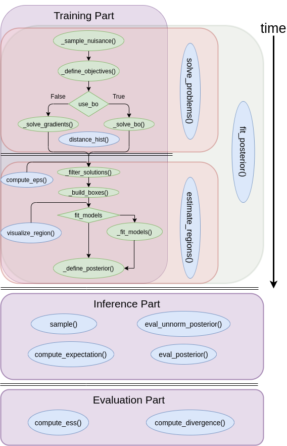
Figure 4: Overview of the ROMC implementation. The training part follows a sequential pattern; the functions in the green ellipses must be called in a sequential fashion for completing the training part and define the posterior distribution. The functions in blue ellipses are the functionalities provided to the user.

3.1.2 Training part

The training part contains the following 6 functionalities:

1. romc.solve_problems(n1, use_bo=False, optimizer_args=None, seed=None)}
   \item \mintinline

   python

romc.estimate_regions(eps_filter,

                      use_surrogate=None, region_args=None,}
      \mintinline

python fit_models=False, fit_models_args=None,

                      eps_region=None, eps_cutoff=None)}
    \item \mintinline

pythonromc.fit_posterior(n1, eps_filter, use_bo=False, optimizer_args=None,

                   seed=None, use_surrogate=None, region_args=None,}
          \mintinline

python fit_models=False, fit_models_args=None,

                   eps_region=None, eps_cutoff=None)}
\item \mintinline

pythonromc.distance_hist(savefig=False, **kwargs)

romc.visualize_region(i, savefig=False)}
\item \mintinline

pythonromc.compute_eps(quantile)

Function (i): Define and solve the optimisation problems

5mm This routine is responsible for (a) drawing the nuisance variables, (b) defining the optimisation problems and (c) solving them using either a gradient-based optimiser or Bayesian optimisation. The aforementioned tasks are done in a sequential fashion, as show in figure 4. The definition of the optimisation problems is performed by drawing $n_{1}$ integer numbers from a discrete uniform distribution $u_{i}\sim\mathcal{U}\{1,2^{32}-1\}$. Each integer $u_{i}$ is the seed used in ELFI’s random simulator. Hence from an algorithmic point-of-view drawing the state of all random variables $\mathbf{v}_{i}$ as described in the previous chapter, traces back to just setting the seed that initialises the state of the pseudo-random generator, before asking a sample from the simulator. Finally, passing an integer number as the argument use_bo=True, chooses the Bayesian Optimisation scheme for obtaining $\boldsymbol{\theta}_{i}^{*}$. In this case, apart from obtaining the optimal points $\boldsymbol{\theta}_{i}^{*}$, we also fit a Gaussian Process (GP) as surrogate model $\hat{d}_{i}$. In the following steps, $\hat{d}_{i}(\boldsymbol{\theta})$ will replace $g_{i}(\boldsymbol{\theta})$ when calling the indicator function.

Function (ii): Construct bounding boxes and fit local surrogate models

romc.estimate_regions(eps_filter,}
      \mintinline

python use_surrogate=None, region_args=None,

                      fit_models=False, fit_models_args=None,}
      \mintinline

python eps_region=None, eps_cutoff=None) This routine constructs the bounding boxes around the optimal points $\boldsymbol{\theta}_{i}^{*}:i=1,2,\ldots,n_{1}$ following Algorithm 3. The Hessian matrix is approximated based on the Jacobian $\mathbf{H}_{i}=\mathbf{J}_{i}^{T}\mathbf{J}_{i}$. The eigenvectores are computed using the function _geev LAPACK. A check is performed so that the matrix $\mathbf{H}_{i}$ is not singular; if this is the case, the eigenvectors are set to be the vectors of the standard Euclidean basis i.e. $\{\mathbf{e_{1}}=(1,0,\ldots),\mathbf{e_{2}}=(0,1,0,\ldots),\text{etc}\}$. Afterwards, the limits are obtained by repeteadly querying the distance function ($g_{i}(\boldsymbol{\theta})$ or $\hat{d}(\boldsymbol{\theta})$) along the search directions. In section LABEL:subsec:developers, we provide some details regarding the way the bounding box is defined as a class and sampling is performed on it.

Function (iii): Perform all training steps in a single call

romc.fit_posterior(n1, eps_filter, use_bo=False, optimizer_args=None,}
          \mintinline

python seed=None, use_surrogate=None, region_args=None,

                fit_models=False, fit_models_args=None,}
          \mintinline

python eps_region=None, eps_cutoff=None) This function merges all steps for constructing the bounding box into a single command. If the user doesn’t want to manually inspect the histogram of the distances before deciding where to set the threshold $\epsilon$, he may call quantile argument must be set to a floating number in the range $[0,1]$ and Function (iv): Plot the histogramm of the optimal points 5mm This function can serve as an intermediate step of manual inspection, for helping the user choose which threshold $\epsilon$ to use. It plots a histogram of the distances at the optimal point $g_{i}(\boldsymbol{\theta}_{i}^{*}):\{i=1,2,\ldots,n_{1}\}$ or $d_{i}^{*}$ in case matplotlib.hist() function; in this way the user may customise some properties of the histogram, such as the number of bins or the range of values.

Function (v): Plot the acceptance region of the objective functions

5mm It can be used as an inspection utility for cases where the parametric space is up to two dimensional. The argument $\verb{}{i}$ is the index of the corresponding optimization problem i.e.\ $i<n_1$. \par\subsubsection*{}{i}$ is the index of the corresponding optimization problem i.e.\ $i<n_1$. \par\subsubsection*Function(vi):Compute$\epsilon$automaticallybasedonthedistributionof$d^{*}$\par\verb{}{romc.compute_eps(quantile)} \vspace{}{romc.compute_eps(quantile)} \vspace5mm\noindent\par\noindent Thisfunctionreturntheappropriatedistancevalue$d_i=κ^*$where$κ= ⌊quantilen ⌋$fromthecollection${ d_i^* } ∀i = {1, …, n}$where$n$isthenumberofacceptedsolutions.Itcanbeusedtoautomatetheselectionofthethreshold$ϵ$,e.g.\ \verb{}{eps=romc.compute_eps(quantile=0.9)}. \par\par\subsubsection*{}{eps=romc.compute_eps(quantile=0.9)}. \par\par\subsubsection*Example\par Herewewillillustratetheaforementionedfunctionalitiesusingthesimple1Dexamplewesetupintheprevioussection.ThefollowingcodesnippetperformsthetrainingpartinELFI.\par\pythoncode n1=500#numberofoptimisationproblemsseed=21#seedforsolvingtheoptimisationproblemseps=.75#thresholdforboundingboxuse_{b}o=False#settoTrueforswitchingtoBayesianoptimisation\par#Trainingstep-by-stepromc.solve_{p}roblems(n1=n1,seed=seed,use_{b}o=use_{b}o)romc.theta_{h}ist(bins=100)romc.estimate_{r}egions(eps=eps)romc.visualize_{r}egion(i=1)\par#Equivalentone-linecommand#romc.fit_{p}osterior(n1=n1,eps=eps,use_{b}o=use_{b}o,seed=seed)\par Asstatedbefore,switchingtotheBayesianoptimisationschemeneedsnothingmorethesettingtheargument\verb{}{use_bo=True}; all the following command remain unchanged. In figure \ref{}{use_bo=True}; all the following command remain unchanged. In figure \reffig:example_{t}raining_{h}istweillustratethedistributionofthedistancesobtainedandtheacceptanceareaofthefirstoptimisationproblem.Weobservethatmostoptimalpointsproducealmostzerodistance.\par\begin{figure}[h]\begin{center}\includegraphics[width=208.13574pt]{./Thesis/images/chapter3/example_theta_dist.png}\includegraphics[width=208.13574pt]{./Thesis/images/chapter3/example_region.png}\end{center}\@@toccaption{{\lx@tag[ ]{{5}}{Histogramofdistancesatthe1Dexample.}}}\@@caption{{\lx@tag[: ]{{Figure 5}}{Histogramofdistancesandvisualisationofaspecificregion.}}}\end{figure}\par$

3.1.3 Inference part

The inference part contains the 4 following functionalities:

1. romc.sample(n2, seed=None)}
   \item \mintinline

   python

romc.compute_expectation(h)

romc.eval_unnorm_posterior(theta)}
\item \mintinline

pythonromc.eval_posterior(theta)

Function (i): Perform weighted sampling

romc.sample(n2)}
\vspace

5mm This is the basic inference utility of the ROMC implementation; we draw $n_{2}$ samples for each bounding box region. This gives a total of $k\times n_{2}$, where $k<n_{1}$ is the number of the optimal points remained after filtering. The samples are drawn from a uniform distribution $q_{i}$ defined over the corresponding bounding box and the weight $w_{i}$ is computed as in equation (2.15). The function stores an romc.result attribute. The romc.result.summary() prints the number of the obtained samples and their mean. A complete overview of these functionalities is provided in ELFI’s official documentation.

Function (ii): Compute an expectation

romc.compute_expectation(h)}
\vspace

5mm This function computes the expectation $E_{p(\boldsymbol{\theta}|\mathbf{y_{0}})}[h(\boldsymbol{\theta})]$ using expression (2.17). The argument Callable.

Function (iii): Evaluate the unnormalised posterior

romc.eval_unorm_posterior(theta, eps_cutoff=False)}
\vspace

5mm This function computes the unnormalised posterior approximation using expression (2.2).

Function (iv): Evaluate the normalised posterior

romc.eval_posterior(theta, eps_cutoff=False)}
\vspace

5mm This function evaluates the normalised posterior. For doing so it needs to approximate the partition function $Z=\int p_{d,\epsilon}(\boldsymbol{\theta}|\mathbf{y_{0}})d\boldsymbol{\theta}$; this is done using the Riemann integral approximation. Unfortunately, the Riemann approximation does not scale well in high-dimensional spaces, hence the approximation is tractable only at low-dimensional parametric spaces. Given that this functionality is particularly useful for plotting the posterior, we could say that it is meaningful to be used for up to $3D$ parametric spaces, even though it is not restricted to that. Finally, for this functionality to work, the elfi.ROMC object.

Example - Sampling and compute expectation

With the following code snippet, we perform weighted sampling from the ROMC approximate posterior. Afterwards, we used some ELFI’s built-in tools to get a summary of the obtained samples. In figure LABEL:fig:example_sampling, we observe the histogram of the weighted samples and the acceptance region of the first deterministic function (as before) alongside with the obtained samples obtained from it. Finally, in the code snippet we demonstrate how to use the h in order to compute firstly the empirical mean and afterwards the empirical variance. In both cases, the empirical result is close to the ground truth $\mu=0$ and $\sigma^{2}=1$. seed = 21 n2 = 50 romc.sample(n2=n2, seed=seed) # visualize region, adding the samples now romc.visualize_region(i=1)