| Effect of internal friction on the coil–stretch transition in turbulent flows | |
| Dario Vincenzia,‡ | |
| Université Côte d’Azur, CNRS, LJAD, Nice, France | |
| A polymer in a turbulent flow undergoes the coil–stretch transition when the Weissenberg number, i.e. the product of the Lyapunov exponent of the flow and the relaxation time of the polymer, surpasses a critical value. The effect of internal friction on the transition is studied by means of Brownian dynamics simulations of the elastic dumbbell model in a homogeneous and isotropic, incompressible, turbulent flow and analytical calculations for a stochastic velocity gradient. The results are explained by adapting the large deviations theory of Balkovsky et al. [Phys. Rev. Lett., 2000, 84, 4765] to an elastic dumbbell with internal viscosity. In turbulent flows, a distinctive feature of the probability distribution of polymer extensions is its power-law behaviour for extensions greater than the equilibrium length and smaller than the contour length. It is shown that although internal friction does not modify the critical Weissenberg number for the coil–stretch transition, it makes the slope of the probability distribution steeper, thus rendering the transition sharper. Internal friction therefore provides a possible explanation for the steepness of the distribution of polymer extensions observed in experiments at large Weissenberg numbers. |
1 Introduction
The coil–stretch transition is the complete unravelling of a polymer that occurs when the polymer is immersed in a non-uniform flow field and the magnitude of the velocity gradient surpasses a critical value. It was initially predicted1, 2 and observed experimentally3, 4 in a laminar extensional flow. The essential features of the coil–stretch transition, such as the strong distortion of the polymer and the associated conformational hysteresis, can be predicted1, 2 by using a model as simple as the elastic dumbbell, which consists of two inertialess beads connected by a spring. Moreover, if the contour length of the polymer is used as fitting parameter, the dumbbell model satisfactorily reproduces the experimental measurements of the end-to-end distance.3, 5, 6, 7 References 8, 9, 10, 11 contain a comprehensive review of single-polymer dynamics in laminar flows.
It was later discovered12, 13, 14 that the coil–stretch transition also occurs in chaotic or turbulent flows, albeit with partially different features. The most notable difference between extensional and turbulent flows is in the probability distribution of the polymer end-to-end distances. In turbulent flows, indeed, the core of the distribution displays a power-law behaviour, which indicates that a wide range of polymer extensions is observed even when the magnitude of the velocity gradient is very large. This feature of the statistics of the end-to-end distance was predicted by applying large-deviations techniques to the dumbbel model in a random flow12 and was observed in both microfluidics experiments14, 15, 16 and numerical simulations of turbulent flows13, 17, 18, 19, 20, 21 (see also Ref. 22, for a review).
The dynamics of a polymer involves internal dissipation processes, generally referred to as ‘internal friction’, which originate from local energy barriers to short-range conformational changes, such as bond rotations, or from interactions between distant segments of the polymer that come close in space.23 In coarse-grained models of elastic polymers, such as the bead–spring chain,24, 25 internal friction has been introduced by adding a linear ‘dashpot’ to each elastic link, which yields a resistive force proportional to the rate of deformation of the link. This idea was proposed by Kuhn and Kuhn 26 under the name of ‘internal viscosity’. The early applications of internal viscosity were mainly concerned with the rheology of viscoelastic fluids (see Refs. 27, 24, 28, 29, 30 and references therein). For instance, internal viscosity is known to cause shear thinning.28 More recently, there has been renewed interest in bead–spring models with internal viscosity thanks to their application to the study of biopolymer dynamics (see, e.g., Refs. 31, 32, 33, 34, 35).
The effect of internal viscosity on polymer stretching has been studied for laminar, planar velocity fields.36, 37, 38, 39 In particular, it was shown in Ref. 36 that a moderate internal viscosity reduces the steady-state end-to-end distance, although without affecting the critical velocity gradient for the coil–stretch transition. In contrast, when the magnitude of internal viscosity exceeds a threshold value, polymers hardly deform. The limiting case of a purely extensional flow was shown to be special, since in such a flow internal viscosity does not modify the steady-state configuration of the polymer. The goal of this study is to examine the effect of internal friction on the coil–stretch transition when the velocity field is turbulent.
It ought to be noted that the notion of internal viscosity has been subject to some criticism,36, 40, 9 for the magnitude of the force exerted by the dashpot is not easily estimated from the molecular properties of the polymer and it has been difficult to find conclusive experimental evidence for the need of internal viscosity in bead–spring chains (the reader is referred to Ref. 41 for a recent introduction on the notion of internal friction and the use of internal viscosity in polymer models). Nevertheless, to the author’s knowledge, the effect of internal dissipation processes in turbulent flows has not been studied yet. Thus, the dumbbell model with internal viscosity provides a simple setting for a qualitative understanding of this phenomenon.
The study consists of Brownian dynamics simulations in three-dimensional homogeneous and isotropic turbulence and focuses on the statistics of polymer extension and the coil–stretch transition. The numerical results are explained by adapting the theory in Ref. 12 to a dumbbell with internal viscosity. In addition, a fully analytical solution for a stochastic velocity gradient supports the interpretation of the results. Finally, the concluding section discusses the experimental evidence for the effect of internal friction on single-polymer dynamics and identifies a phenomenon, namely the steepness of the probablity distribution of the end-to-end distances, that can be attributed to internal friction and not to other forces usually included in bead-spring chains, such as hydrodynamic and excluded-volume interactions or a conformation-dependent drag.
2 Model and methods
2.1 Elastic dumbbell with internal viscosity
The polymer is described as an elastic dumbbell. The extension and orientation are specified by the vector that connects the two beads and represents the end-to-end separation vector of the polymer. Internal viscosity is introduced in the dumbbell model by adding the resistive force to the equation for (see Refs. 26, 28). Here and is termed the internal viscosity coefficient. The resistive force is parallel to and has a magnitude proportional to . Thus, for a finitely extensible nonlinear elastic (FENE) dumbbell with internal viscosity the evolution equation for the connector vector is42, 43
| (1) |
with
| (2a) | |||||
| (2b) | |||||
| (2c) | |||||
where and summation over repeated indices is understood, is the relaxation time of the polymer, is its contour length, is the drag coefficient of the beads, is the Boltzmann constant, is temperature, is the velocity gradient at the position of the center of mass, and is the three-dimensional Brownian motion [in Eq. (1) the noise term is interpreted in the Itô sense43]. The equilibrium length of the dumbbell, defined as the standard deviation of for , is .
The parameter describes the ratio of internal viscosity to the hydrodynamic drag. The usual FENE dumbbell model is recovered for , whereas for infinite Eq. (1) yields the rigid dumbbell model.28 In the literature, is typically taken between 0 and 10.
The balance between polymer stretching and relaxation is measured by the Weissenberg number, which in a chaotic flow is commonly defined as , where is the maximum Lyapunov exponent of the flow, i.e. the average exponential rate at which fluid particles separate.
Here Eq. (1) is studied under the assumption that is the gradient of a turbulent velocity field. It is worth mentioning that even though Eq. (1) assumes a linear velocity field, it remains appropriate for turbulent flows, because the length of a polymer is generally shorter than the viscous dissipation scale, which is the smallest length scale in such flows.
2.2 Brownian dynamics simulations
The effect of internal viscosity is studied by using a database of Lagrangian trajectories in homogeneous and isotropic, incompressible turbulence generated at ICTS, Bangalore44. Although an isotropic turbulent flow has zero mean strain rate, line elements are stretched exponentially with an asymptotic rate . Thus, a polymer in an isotropic turbulent flow experiences strong stretching events that can unravel it completely.12, 45, 19 The database was obtained by tracking the positions of fluid particles and calculating along their trajectories in a direct numerical simulation of the three-dimensional Navier–Stokes equations over a periodic cube and at Taylor-microscale Reynolds number (see Ref. 44 for more details). The time series of is then inserted into Eq. (1). This procedure assumes that the centre of mass of a polymer moves along a fluid trajectory; therefore the effect of thermal noise on the motion of the centre of mass is disregarded. Such an assumption is justified in a turbulent flow, because thermal diffusion is negligible compared to turbulent diffusion.
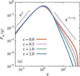
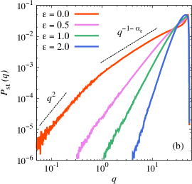
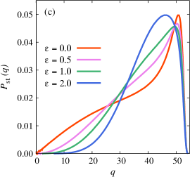
For the numerical integration of Eq. (1), Ref. 41 proposes a semi-implicit predictor–corrector scheme, which is adapted from an analogous algorithm initially derived for .25 However, in the present setting the Euler–Maruyama method supplemented with a rejection algorithm25 proved accurate enough to prevent extensions greater than (for and the largest value of Wi—the least favourable case—only 0.02% of the time steps were rejected). In the Lagrangian database, the velocity gradient was saved at a time interval . The time step used for the integration of Eq. (1) is ; a linear interpolation between two subsequent values of the velocity gradient is therefore required. In Sect. 3.1, the contour length is and , , , are such that is unity. The ratio is thus comparable to that of long DNA molecules4 and is the same as that used in Refs. 45, 19. In Sect. 3.3, is taken unrealistically large, namely , in order accurately to resolve the power-law behaviour of the distribution of . The Weissenberg number is varied between 0.05 and 8, while is taken between 0 and 2.
3 Results and discussion
3.1 Polymer stretching in isotropic turbulence: the effect of internal viscosity
The statistics of polymer stretching is described in terms of the stationary probability density function (PDF) of the polymer end-to-end distance, here denoted as . It was already mentioned in Sect. 1 that if , analytical,12 experimental,14, 15, 16 and numerical13, 17, 18, 19, 20, 21 studies of the dumbbell model have shown that behaves as a power of for , with a slope that is negative for small Wi, motonically increases as a function of Wi, and crosses when the Weissenberg number takes the critical value (note that the present definition of , and hence of Wi, differs by a factor of 2 from that used in some of the references cited above). Thus, in the limit (linear polymer), is no longer normalisable for , and this is interpreted as the indication of the coil–stretch transition occurring at . The power-law behaviour of means that the PDF is not dominated by a peak about its mean, but the distribution of polymer extensions is broad. The transition is characterized by a rapid increase of the mean extension and a sharp maximum in the coefficient of variation of , defined as , where is the standard deviation of (see Refs. 14, 19, 46). The latter behaviour is a further indication of the breadth of the distribution and the heterogeineity of polymer configurations in a turbulent flow.
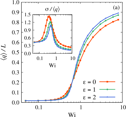
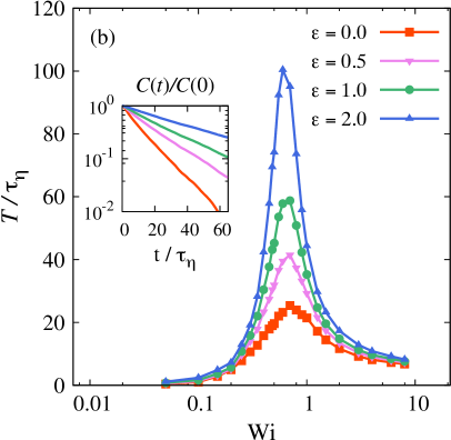
Figure 1 shows that, in the presence of internal viscosity, continues to behave as a power of for intermediate extensions, but the slope of the power law changes significanly with . Internal viscosity indeed makes the power steeper: the PDF falls faster than for at small Wi and rises faster at large Wi. As a consequence, the mean polymer extension displays a sharper transition from the coiled to the stretched state as is increased, and its asymptotic value is larger at higher (see Fig 2(a)). At the same time, the dispersion of the PDF around the mean is reduced by internal viscosity, as is quantified by a systematically smaller coefficient of variation for (inset of Fig. 2(a)).
This behaviour of may be inferred from the fact that, in a turbulent flow, large deviations from the mean extension are the cumulative result of strong fluctuations of the velocity gradient, and the effect of internal viscosity is to attenuate the response of the polymer to sudden variations in the velocity gradient. However, a rigorous explanation of this phenomenon will be given in the following sections.
The coil–stretch transition also manifests itself in a significant increase of the correlation time of polymer the end-to-end distance.19 A related phenomenon is the slowing down of the equilibration dynamics of the polymer in the flow.47 If is the autocorrelation function of the end-to-end distance, the correlation time is defined as . The inset of Fig. 2(b) shows that decays approximately as an exponential function, as was already observed for (see Ref. 19). However, internal viscosity strongly amplifies the aforementioned increase of the correlation time near the coil–stretch transition: displays a higher and higher peak near as grows (in Fig. 2(b), time is rescaled by the Kolmogorov time , which is the time scale associated with viscous dissipation in turbulent flows).
Finally, the orientation dynamics of polymers in isotropic turbulence has also attracted some attention.19, 20, 48 Internal viscosity obviously does not affect the orientation of a polymer directly, because is parallel to . However, it may in principle do so indirectly, since it modifies the statistics of .The numerical results (not shown) indicate that internal viscosity causes a mild reduction of the alignment of the polymer with the vorticity only for Wi smaller than and close to . The effect on the orientation dynamics is otherwise negligible.
3.2 An exactly solvable model
The stationary PDF of can be calculated exactly if the turbulent velocity gradient is modelled as a a stochastic tensor with suitable statistical properties. In the Batchelor regime of the three-dimensional Kraichnan model,49 is an isotropic traceless tensorial white noise, which means that is Gaussian, has zero mean, and two-time correlation
| (3) |
with . This stochastic model of the velocity gradient has been widely used in the study of turbulent transport 49 and was applied for the first time to single-polymer dynamics in Ref. 50. With this choice of , the velocity gradient plays the role of a multiplicative noise in the second term on the right hand side of Eq. (1) and is interpreted in the Stratonovich sense.50, 49
By using the methods presented in Ref. 51, it can be shown that if is as above, then the PDF of the vector , denoted as , satisfies the Fokker–Planck equation
| (4) |
with drift and diffusion coefficients
| (5) |
where , , have been defined in Eqs. (2). Summation over repeated indices is assumed also in this section. The change to spherical coordinates transforms Eq. (4) into a Fokker–Planck equation for with coefficients:
and (see Ref. 52, p. 88, for the transformation rules of a Fokker–Planck equation under a change of variables). Taking into account the statistical isotropy of the flow, it is now assumed that the stationary PDF of is of the form . By replacing this expression into the Fokker–Planck equation for , it is then found that satisfies the equation
| (6) |
which is solved with a reflecting boundary condition in . This implies that in the steady state the probability current vanishes everywhere.52 The solution of Eq. (6) corresponding to zero probability current is52 , whence the analytical expression of is
| (7) |
with
| (8) |
If is set to zero, the above PDF reduces to that found in Ref. 46 for a polymer with zero internal viscosity in the Batchelor–Kraichnan flow. At small , the PDF is proportional to , because the dynamics is dominated by thermal fluctuations. At very large , the last term in Eq. (7), which originates from the nonlinear elastic force, introduces a cut-off at the length . For , the stationary PDF of behaves as with
| (9) |
The factor has the effect of reducing the slope of for and increasing it for . This makes narrower and the coil–stretch transition sharper, although it does not modify , which is defined as the value of Wi at which vanishes. Thus, the stochastic model captures the effect of internal viscosity on the steady-state statistics of polymer extension as observed in the Brownian dynamics simulations and provides an analytical tool for the study of internal viscosity in turbulent flows.
3.3 Predictions for a general random flow
The behaviour of observed in the Brownian dynamics simulations and reproduced by the stochastic model can be predicted for a general random flow by invoking the theory in Ref. 12. This is briefly recalled below in the version provided in Ref. 17, which uses the generalized Lyapunov exponents.
Let be a line element in a random flow. Its time evolution is given by the equation , which in turn yields the following equation for the length of the line element:
| (10) |
with . The -th generalized Lyapunov exponent is defined as53, 54
| (11) |
where denotes the average over the statistics of the velocity field. represents the rate of exponential growth of the -th moment of . It is a positive and convex function of and satisfies , where is the space dimension. In addition, .
References 12 and 17 express in terms of (or its Legendre transformation). It is first observed that if and thermal noise is disregarded, the end-to-end distance and the orientation of a linear polymer evolve according to the following equations:55, 12
| (12a) | |||||
| (12b) | |||||
with . The similarity between Eq. (12a) and Eq. (10) makes it clear that the statistics of must be related to the generalized Lyapunov exponents of the flow. Extensions much greater than are observed after the polymer has experienced large values of . Thus, is expressed in terms of by writing the first of Eqs. (12a) in integral form, and then the probability of large values of is approximated with its large-deviations form to find:
| (13) |
for . The value of is therefore sought as the nonzero intersection of the straight line with the function . By using the aforementioned properties of as a function of , it is easy to see that is positive for small Wi and decreseas with Wi, until it vanishes for . It then becomes negative for . Close to , the generalized Lyapunov exponent can be expanded as with . This expansion allows the explicit calculation of for Wi near to :
| (14) |
In particular, the latter expression shows that . Finally, the limit of for infinite Wi is obtained when the straight line is parallel to the horizontal axis, whence .
It is worth mentioning that Eq. (13) holds under very mild assumptions on the random flow, namely that the correlation time of is finite.12 Moreover, even though Eq. (13) is derived for a dumbbell, Ref. 19 has shown that the steady-state statistics of the end-to-end distance is the same for a dumbbell and a chain with multiple beads, provided that a suitable mapping between the parameters of the two systems is applied. Hence the validity of Eq. (13) is not restriced to the dumbbell model.
It is now discussed how internal viscosity modifies the above predictions. If , the analogue of Eq. (12a) can be obtained by multiplying Eq. (1) by , neglecting the noise term, summing over , and dividing by to find:
| (15) |
Constrastingly, Eq. (12b) is unchanged. Therefore, for , the time evolution of is the same as that of a polymer with , provided that is multiplied by and is rescaled by the same quantity. It follows immediately that must display a power-law behaviour also in the presence of internal viscosity:
| (16) |
with an exponent that can be determined as follows. Rescaling by is equivalent to considering the evolution of in a flow with generalized Lyapunov exponents . This can be seen by noting that the solution of Eq. (10) is ; if this expression is replaced into Eq. (11), it follows that considering a flow with a rescaled is the same as taking a moment of of a rescaled order in the original flow. Hence, the equivalent of Eq. (13) for is
| (17) |
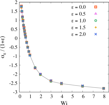
Comparing Eq. (17) with Eq. (13) finally yields
| (18) |
Therefore, the effect of internal viscosity on the PDF of polymer extensions is to multiply by a factor of . Since the criterion for the coil–stretch transition in random flows is , internal viscosity does not modify the critical Weissenberg number. However, the statistics of is affected. Indeed, when , i.e. for , whereas in the opposite case. Thus, below the coil–stretch transition the probability of large extensions is depleted by internal viscosity; above the transition it is the small extensions that are disfavoured. As a result, the mean extension is reduced when Wi is below and increased for , while the width of the PDF of the extension is systematically decreased by internal viscosity. The coil–stretch transition therefore becomes sharper with increasing . Figure 3 clearly illustrates the validity of Eq. (18) by showing rescaled by from the Brownian dynamics simulations described in Sect. 2.2 he value of is estimated by fitting for with a power law (in order to obtain an accurate estimate, here the ratio of and is taken larger than in Sect. 3.1, i.e. ).
In the Batchelor–Kraichnan flow studied in Sect. 3.2, is exactly quadratic for all (see Ref. 49). Hence the expression for given in Eq. (14) holds for all Wi and not only near the coil–stretch transition. In addition, for this flow. 49 Therefore, Eq. (9) is an explicit example of the general relation given in Eq. (18).
4 Summary and conclusions
The effect of internal friction on polymer stretching in turbulent flows has been studied by considering an elastic dumbbell with a linear dashpot. The results are based on Brownian dynamics simulations using a database of fluid trajectories in isotropic turbulence, an exact solution for a stochastic velocity gradient, and a generalization of the large deviations approach of Ref. 12 that takes internal viscosity into account. Although it does not modify the critical Weissenberg number for the coil–stretch transition, internal viscosity strongly affects the statistics of polymer extension in two opposite ways below and above the transition. Its effect is indeed to multiply by a factor of . This depletes the probability of large extensions below the transition and the probability of small extensions above the transition, thus leading to a sharpening of the transition itself. Internal viscosity also enhances the peak of the correlation time of the extension near , whereas it has a negligible effect on the orientation statistics of the polymer.
It remains to consider the question of the experimental evidence for the phenomenon described here. If internal viscosity is disregarded, the theory12 predicts that, in the limit of very large Weissenberg numbers, should tend to , and hence, in a three dimensional flow, for . However, experiments 16 show PDFs as steep as when the Weissenberg number is large. The theory therefore does not explain the shape of in the large-Wi regime. Contrastingly, if internal viscosity is taken into account, Eq. (18) implies that and hence as . Thus, internal friction provides a possible explanation for the steep behaviour of observed in experiments at large Wi. Moreover, the experimental slope is recovered by taking , a value of which falls in the range typically considered in studies of internal friction.
It is interesting to note that other forces that are usually included in bead-spring chain models cannot explain the steepness of for large Wi. Hydrodynamic interactions between the beads have the effect of delaying the unravelling of the polymer, and once this is sufficiently stretched, they become negligible. Therefore, in a turbulent flow, hydrodynamic interactions reduce the probability of large extensions for all Wi. Excluded-volume interactions are short-range and do not impact the statistics of large polymer extensions. A conformation-dependent drag, which interpolates bewteen the drag coefficient of a sphere in the coiled state and that of a thin cylinder in the stretched state,2 impacts the dynamics of the polymer around the coil–stretch transition, but has little effect at large Wi, when most of the polymers are highly stretched anyway.4, 7, 47 In particular, by using the analytical results of Ref. 47, it is easy to check that, in the Batchelor–Kraichnan flow, as , even if the drag coefficient of the polymer depends on its conformation. Thus, the present study identifies a phenomenon that is the unambiguous result of internal friction.
Acknowledgements
The author is grateful to S. S. Ray for providing access to his database of turbulent Lagrangian trajectories and to J. R. Picardo for useful suggestions. The Brownian dynamics simulations were perfomed at Centre de Calculs Interactifs of Université Côte d’Azur.
References
- P.-G. de Gennes 1974 P.-G. de Gennes, J. Chem. Phys., 1974, 60, 5030–5042.
- Hinch 1975 E. J. Hinch, Colloques Internationaux du CNRS, Éditions du CNRS, Paris, 1975, vol. 233, pp. 241–247.
- Perkins et al. 1997 T. Perkins, D. E. Smith and S. Chu, Science, 1997, 276, 2016–2021.
- Schroeder et al. 2003 C. M. Schroeder, H. P. Babcock, E. S. G. Shaqfeh and S. Chu, Science, 2003, 301, 1515–1519.
- Larson et al. 1997 R. G. Larson, T. T. Perkins, D. E. Smith and S. Chu, Phys. Rev. E, 1997, 55, 1794–1797.
- Larson et al. 1999 R. G. Larson, H. Hu, D. E. Smith and S. Chu, J. Rheol., 1999, 43, 267–304.
- Schroeder et al. 2004 C. M. Schroeder, E. S. G. Shaqfeh and S. Chu, Macromolecules, 2004, 37, 9242–9256.
- Nguyen and Kausch 1999 Flexible Polymer Chain Dynamics in Elongational Flow, ed. T. Q. Nguyen and H.-H. Kausch, Springer, Berlin Heidelberg, 1999.
- Larson 2005 R. G. Larson, J. Rheol., 2005, 49, 1–70.
- Shaqfeh 2005 E. S. G. Shaqfeh, J. Non-Newtonian Fluid Mech., 2005, 130, 1–28.
- Schroeder 2018 C. M. Schroeder, J. Rheol., 2018, 62, 371–403.
- Balkovsky et al. 2000 E. Balkovsky, A. Fouxon and V. Lebedev, Phys. Rev. Lett., 2000, 84, 4765–4768.
- Eckhardt et al. 2002 B. Eckhardt, J. Kronjäger and J. Schumacher, Comput. Phys. Commun., 2002, 147, 538–543.
- Gerashchenko et al. 2005 S. Gerashchenko, C. Chevallard and V. Steinberg, Europhys. Lett., 2005, 71, 221–227.
- Liu and Steinberg 2010 Y. Liu and V. Steinberg, Europhys. Lett., 2010, 90, 44005.
- Liu and Steinberg 2014 Y. Liu and V. Steinberg, Macromol. Symp., 2014, 337, 34–43.
- Boffetta et al. 2003 G. Boffetta, A. Celani and S. Musacchio, Phys. Rev. Lett., 2003, 91, 034501.
- Puliafito and Turitsyn 2005 A. Puliafito and K. Turitsyn, Physica D, 2005, 211, 9–22.
- Watanabe and Gotoh 2010 T. Watanabe and T. Gotoh, Phys. Rev. E, 2010, 81, 066301.
- Bagheri et al. 2012 F. Bagheri, D. Mitra, P. Perlekar and L. Brandt, Phys. Rev. E, 2012, 86, 056314.
- Gupta et al. 2015 A. Gupta, P. Perlekar and R. Pandit, Phys. Rev. E, 2015, 91, 033013.
- Benzi and Ching 2018 R. Benzi and E. S. C. Ching, Annu. Rev. Condens. Matter Phys., 2018, 9, 163–181.
- de Gennes 1979 P.-G. de Gennes, Scaling Concepts in Polymer Physics, Cornell University Press, Ithaca, NY, 1979.
- Bird et al. 1987 R. B. Bird, C. F. Curtiss, R. C. Armstrong and O. Hassager, Dynamics of Polymeric Liquids, Wiley, 1987, vol. 2.
- Öttinger 1996 H. C. Öttinger, Stochastic Processes in Polymeric Fluids, Springer, Berlin, 1996.
- Kuhn and Kuhn 1945 W. Kuhn and H. Kuhn, Helv. Chim. Acta, 1945, 28, 1533–1579.
- Manke and Williams 1985 C. W. Manke and M. C. Williams, Macromolecules, 1985, 18, 2045–2051.
- Larson 1988 R. G. Larson, Constitutive Equations for Polymer Melts and Solutions, Butterworth Publishers, Stoneham, MA, 1988.
- Bird and Öttinger 1992 R. B. Bird and H. C. Öttinger, Annu. Rev. Phys. Chem., 1992, 43, 371–406.
- Ryder and Yeomans 2006 J. F. Ryder and J. M. Yeomans, J. Chem. Phys., 2006, 125, 194906.
- Portman et al. 2001 J. J. Portman, S. Takada and P. G. Wolynes, J. Chem. Phys., 2001, 114, 5082–5096.
- Khatri and McLeish 2007 B. S. Khatri and T. C. B. McLeish, Macromolecules, 2007, 40, 6770–6777.
- Schulz et al. 2012 J. C. F. Schulz, L. Schmidt, R. B. Best, J. Dzubiella and R. R. Netz, J. Am. Chem. Soc., 2012, 134, 6273–6279.
- Cheng et al. 2013 R. R. Cheng, A. T. Hawk and D. E. Makarov, J. Chem. Phys., 2013, 138, 074112.
- Samanta and Chakrabarti 2016 N. Samanta and R. Chakrabarti, Physica A, 2016, 450, 165–179.
- Fuller and Leal 1981 G. G. Fuller and L. G. Leal, J. Non-Newtonian Fluid Mech., 1981, 8, 271–310.
- Manke and Williams 1989 C. W. Manke and M. C. Williams, J. Rheol., 1989, 33, 949–978.
- Schieber 1993 J. D. Schieber, J. Rheol., 1993, 37, 1003–1027.
- Wedgewood 1993 L. E. Wedgewood, Rheol. Acta, 1993, 32, 405–4178.
- Doyle and Shaqfeh 1998 P. S. Doyle and E. S. G. Shaqfeh, J. Non-Newtonian Fluid Mech., 1998, 76, 43–78.
- Kailasham et al. 2018 R. Kailasham, R. Chakrabarti and J. R. Prakash, J. Chem. Phys., 2018, 149, 094903.
- Schieber 1992 J. D. Schieber, J. Non-Newtonian Fluid Mech., 1992, 45, 47–61.
- Hua and Schieber 1995 C. C. Hua and J. D. Schieber, J. Non-Newtonian Fluid Mech., 1995, 56, 307–332.
- James and Ray 2017 M. James and S. S. Ray, Sci. Reports, 2017, 7, 12231.
- Jin and Collins 2007 S. Jin and L. R. Collins, New J. Phys., 2007, 9, 360.
- Martins Afonso and Vincenzi 2005 M. Martins Afonso and D. Vincenzi, J. Fluid Mech., 2005, 540, 99–108.
- Celani et al. 2006 A. Celani, A. Puliafito and D. Vincenzi, Phys. Rev. Lett., 2006, 97, 118301.
- Vincenzi et al. 2015 D. Vincenzi, P. Perlekar, L. Biferale and F. Toschi, Phys. Rev. E, 2015, 92, 053004.
- Falkovich et al. 2001 G. Falkovich, K. Gawȩdki and M. Vergassola, Rev. Mod. Phys., 2001, 73, 913–975.
- Chertkov 2000 M. Chertkov, Phys. Rev. Lett., 2000, 84, 4761–4764.
- E. L. C. VI M. Plan et al. 2016 E. L. C. VI M. Plan, A. Ali and D. Vincenzi, Phys. Rev. E, 2016, 94, 020501(R).
- Risken 1989 H. Risken, The Fokker–Planck Equation, Springer, Berlin, 1989.
- Crisanti et al. 1993 A. Crisanti, G. Paladin and A. Vulpiani, Products of Random Matrices in Statistical Physics, Springer, Berlin, 1993.
- Cecconi et al. 2010 F. Cecconi, M. Cencini and A. Vulpiani, Chaos: from Simple Models to Complex Systems, World Scientific, Singapore, 2010.
- Olbricht et al. 1982 W. L. Olbricht, J. M. Rallison and L. G. Leal, J. Non-Newtonian Fluid Mech., 1982, 10, 291–318.