U(1) CS Theory vs SL(2) CS Formulation: Boundary Theory and Wilson Line
Xing Huang^a,b,c , Chen-Te Ma^d,e,f,g,h , Hongfei Shu^i,j,k,l , and
Chih-Hung Wu^m
a Institute of Modern Physics, Northwest University, Xi’an 710069, China.
^b Shaanxi Key Laboratory for Theoretical Physics Frontiers, Xi’an 710069, China.
^c NSFC-SPTP Peng Huanwu Center for Fundamental Theory, Xi’an 710127, China.
^d Asia Pacific Center for Theoretical Physics,
Pohang University of Science and Technology, Pohang 37673, Gyeongsangbuk-do, South Korea.
^e Guangdong Provincial Key Laboratory of Nuclear Science,
Institute of Quantum Matter, South China Normal University, Guangzhou 510006, Guangdong, China.
^f School of Physics and Telecommunication Engineering,
South China Normal University, Guangzhou 510006, Guangdong, China.
^g Guangdong-Hong Kong Joint Laboratory of Quantum Matter,
Southern Nuclear Science Computing Center, South China Normal University, Guangzhou 510006, China.
^h The Laboratory for Quantum Gravity and Strings,
Department of Mathematics and Applied Mathematics,
University of Cape Town, Private Bag, Rondebosch 7700, South Africa.
ⁱ Beijing Institute of Mathematical Sciences and Applications (BIMSA), Beijing, 101408, China.
^j Yau Mathematical Sciences Center (YMSC), Tsinghua University, Beijing, 100084, China.
^k Nordita, KTH Royal Institute of Technology and Stockholm University,
Roslagstullsbacken 23, SE-106 91 Stockholm, Sweden.
^l Department of Physics, Tokyo Institute of Technology, Tokyo, 152-8551, Japan.
^m Department of Physics, University of California, Santa Barbara, CA 93106, USA.

We first derive the boundary theory from the U(1) Chern-Simons theory. The boundary action on an $n$-sheet manifold appears from its back-reaction of the Wilson line. The reason is that the U(1) Chern-Simons theory can provide an exact effective action when introducing the Wilson line. The Wilson line in the pure AdS₃ Einstein gravity is equivalent to entanglement entropy in the boundary theory up to classical gravity. The U(1) Chern-Simons theory deviates by a self-interaction term from the gauge formulation on the boundary. We also compare the Hayward term in the SL(2) Chern-Simons formulation to the Wilson line approach. Introducing two wedges can reproduce the entanglement entropy for a single interval at the classical level. We propose quantum generalization by combining the bulk and Hayward terms. The quantum correction of the partition function vanishes. In the end, we calculate the entanglement entropy for a single interval. The pure AdS₃ Einstein gravity theory shows a shift of central charge by 26 at the one-loop level. The U(1) Chern-Simons theory does not show a shift from the quantum effect. The result is the same in the weak gravitational constant limit. The non-vanishing quantum correction shows that the Hayward term is incorrect.

1 Introduction

The goal of studying emergent spacetime is to obtain the bulk geometry from other equivalent descriptions. Since Einstein gravity theory is not renormalizable, people expect that Einstein gravity theory may not be a fundamental theory. One promising approach is the Holographic Principle [1, 2, 3, 4, 5]. This principle states that the physical degrees of freedom in Quantum Gravity are all on its boundary. One candidate for perturbative Quantum Gravity, String Theory, provided a conjecture, the Anti-de Sitter/Conformal Field Theory Correspondence (AdS/CFT correspondence). String theory in the $(d+1)$-dimensional AdS manifold is dual to CFT_d. It is a surprising fact that a gravitational theory is calculable. Furthermore, the Ryu-Takayanagi prescription shows that the surface with a minimum area (minimum surface) in AdS_d+1 contains the boundary information (entanglement entropy) [6, 7]. Therefore, this seems to imply Quantum Entanglement generates the bulk spacetime.

The calculation of quantum entanglement quantities, in general, relies on the $n$-sheet manifold with the analytical continuation of $n$ [8], which is hard to calculate. The minimum surface provides a simplified way to study entanglement entropy [9, 10]. However, to confirm the observation, it is necessary to perform a perturbation in a boundary theory to probe the quantum regime of bulk gravity theory. To obtain exact properties in Quantum Entanglement, we study Chern-Simons (CS) Theory [11].

We begin with the AdS₃ Einstein gravity theory. Because 3d pure Einstein gravity theory (metric formulation) does not have local degrees of freedom [12]. The metric formulation is equivalent to an SL(2) CS formulation (gauge formulation) up to the classical level [13]. Although the metric formulation is not equivalent to the gauge formulation due to its measure, the renormalizable gauge formulation is convenient for computation in the quantum regime [14, 15].

The absence of local degrees of freedom implies that one can derive the boundary action. The first derivation showed that the boundary theory is the Liouville theory [16], CFT. Because the Liouville theory does not have a normalizable vacuum, it contradicts the bulk theory [17]. Indeed, it is a classical action because people do not consider the measure. Recently, due to a proper consideration for including the measure into the boundary theory, the 2d Schwarzian theory appears. This theory has the expected SL(2) reparametrization gauge redundancy [18]. The 2d Schwarzian theory does not have conformal symmetry. People should expect the result due to conformal anomaly.

The first question is to find the gauge version of the minimum surface. Because the Wilson lines constitute all operators in the gauge formulation, Wilson line is shown to be a probe of holographic entanglement [19, 20]. In the AdS/CFT correspondence, it is not a simple task to study the minimum surfaces at an operator level. The CS theory is a simple system for avoiding difficulty. Hence studying the gauge formulation of pure AdS₃ Einstein gravity theory should give a clue to emergent spacetime.

The co-dimension two Hayward term [21] was recently connected with the entanglement entropy at the classical gravity level [22]. The basic idea is to introduce a Euclidean bulk manifold with two boundaries that are not smoothly junctioned. When gluing two boundary surfaces at a co-dimension two wedge, the junction conditions induce an additional Hayward term. It ensures a well-posed variational principle. The Hayward term induces the wedge contribution to the partition function [22, 23]. This contribution implies the equivalence with the co-dimension two cosmic brane action with a suitable tension [22, 23]. The approach effectively introduces the back-reaction on the replica orbifold that generates a conical geometry [24]. The Hayward term is a gravitational action rather than an auxiliary tool (cosmic brane action). Therefore, we are interested in understanding how the wedge term arises in the SL(2) CS formulation.

In this paper, we study holographic entanglement entropy in the gauge formulation. We calculate entanglement entropy and Wilson line with the quantum correction. The SL(2) CS formulation has exact solutions to the boundary effective action and the partition function [18]. However, it does not have an exact solution when introducing the Wilson lines. Introducing the Wilson line produces a back-reaction to generate an $n$-sheet manifold [19]. The additional term related to the Wilson line vanishes in the limit $n\rightarrow 1$. Hence this does not produce a problem but relies on whether the limit or a smooth solution exists. We will first study a similar but simpler system, U(1) CS theory. Furthermore, to understand whether the Hayward term is a suitable proposal for obtaining entanglement entropy, we study the Hayward term in the SL(2) CS formulation. To summarize our results:

• We derive the boundary action of U(1) CS theory. The result shows a combination of left- and right-chiral non-interacting scalar field theories [25]. This theory can be rewritten from the non-interacting scalar field theory [26]. Introducing the Wilson lines is equivalent to deforming the chiral scalar fields and does not change the bulk theory. Obtaining the non-interacting scalar field theory on an $n$-sheet manifold is necessary to deform the boundary condition. We perform this study by first deforming the chiral scalar fields and choosing the $n$-sheet background. It establishes an exact correspondence between the Wilson line and entanglement entropy. This study shows that deformation is crucial for the relation between the Wilson line and entanglement entropy.

• We derive the boundary action for the SL(2) CS formulation. The boundary action is similar to the U(1) case (but it has additional terms for the interaction). We can choose the weak gravitational constant limit to truncate the self-interaction. The non-trivial deformation is again necessary for building an exact correspondence between the Wilson line and entanglement entropy as in the U(1) CS theory. Indeed, this establishes the “minimum surface=entanglement entropy” prescription with the quantum fluctuation of gauge fields for studying the quantum deformation of minimum surface [15].

• We use the boundary term [27] to obtain the co-dimension two Hayward term. This method is the same as in the metric formulation. Two wedges forming a single interval on the boundary can reproduce the entanglement entropy at the classical level. Combining the bulk and Hayward terms does not generate quantum correction. It is inconsistent with the one-loop exact calculation of the entanglement entropy. Hence we conclude that the quantum generalization does not provide a suitable description of the entanglement entropy.

• We calculate the entanglement entropy for a single interval in the SL(2) CS formulation. It shows an exact shift of central charge by 26. The shift should result from the additional interacting term since the U(1) CS theory does not generate the shifting. This result supports the equivalence of the two theories in the weak gravitational constant limit. The U(1) CS theory and the SL(2) CS formulation do not have the same number on gauge fields. The boundary degrees of freedom are the same. Hence showing equivalence is a non-trivial result.

The organization of this paper is as follows: We derive the boundary action and study its dual in Sec. 2. The duality provides the relation between the Wilson line and entanglement entropy. We then consider the boundary action, the building of “minimum surface=entanglement entropy” for SL(2) CS formulation, and the set-up of the co-dimension two Hayward term in Sec. 3. We calculate the entanglement entropy for a single interval in SL(2) CS formulation at one loop in Sec. 4. In the end, we have our concluding remarks in Sec. 5. We give the details of the one-loop correction for Rényi entropy in Appendix A.

2 U(1) CS Theory

To provide a clear picture of the bulk-boundary correspondence, we first introduce U(1) CS theory. We derive the boundary action in U(1) CS theory. We then introduce the Wilson lines for a study of entanglement entropy.

2.1 Action

The action for the U(1) CS theory in the Lorentzian manifold is given by

$$S_{\mathrm{U}(1)}$$ (1)

$$= \frac{k}{2\pi}\int d^{3}x\ \bigg{(}A_{t}F_{r\theta}-\frac{1}{2}\big{(}A_{r}\partial_{t}A_{\theta}-A_{\theta}\partial_{t}A_{r}\big{)}\bigg{)}$$

$$-\frac{k}{2\pi}\int d^{3}x\ \bigg{(}\bar{A}_{t}\bar{F}_{r\theta}-\frac{1}{2}\big{(}\bar{A}_{r}\partial_{t}\bar{A}_{\theta}-\bar{A}_{\theta}\partial_{t}\bar{A}_{r}\big{)}\bigg{)}$$

$$-\frac{k}{4\pi}\int dtd\theta\ \frac{E_{t}^{+}}{E_{\theta}^{+}}A_{\theta}^{2}$$

$$+\frac{k}{4\pi}\int dtd\theta\ \frac{E_{t}^{-}}{E_{\theta}^{-}}\bar{A}_{\theta}^{2}.$$

The boundary conditions become:

$$(E_{\theta}^{+}A_{t}-E_{t}^{+}A_{\theta})|_{r\rightarrow\infty}=0;\qquad(E_{\theta}^{-}\bar{A}_{t}-E_{t}^{-}\bar{A}_{\theta})|_{r\rightarrow\infty}=0.$$ (2)

The $t$, $r$, $\theta$ are the polar coordinates, and the ranges are given by:

$$-\infty<t<\infty;\qquad 0<r<\infty;\qquad 0<\theta\leq 2\pi.$$ (3)

The boundary zweibein is defined by:

$$E^{+}\equiv E^{\theta}+E^{t};\qquad E^{-}\equiv E^{\theta}-E^{t}.$$ (4)

We also define the component of the boundary zweibein as the following:

$$E^{+}_{\theta}d\theta\equiv E^{\theta};\qquad E^{+}_{t}dt\equiv E^{t};\qquad E^{-}_{\theta}d\theta\equiv E^{\theta};\qquad E^{-}_{t}dt\equiv-E^{t}.$$ (5)

The boundary metric in terms of the boundary zweibein is

$$g_{\tilde{\mu}\tilde{\nu}}\equiv\frac{1}{2}(E_{\tilde{\mu}}^{+}E_{\tilde{\nu}}^{-}+E_{\tilde{\mu}}^{-}E_{\tilde{\nu}}^{+}).$$ (6)

The indices of boundary spacetime are $\tilde{\mu}=t,\theta$. The notation for the $x^{+}$ and $x^{-}$ is:

$$x^{+}=t+\theta;\qquad x^{-}=t-\theta.$$ (7)

We can do the integration by part

$$\frac{k}{2\pi}\int d^{3}x\ A_{t}F_{r\theta}=\frac{k}{4\pi}\int d^{3}x\ \bigg{(}A_{t}\partial_{r}A_{\theta}-A_{t}\partial_{\theta}A_{r}-A_{\theta}\partial_{r}A_{t}+A_{r}\partial_{\theta}A_{t}\bigg{)}$$ (8)

to show the familiar CS form

$$S_{\mathrm{U(1)}}=\frac{k}{4\pi}\int d^{3}x\ \epsilon^{\mu\nu\rho}A_{\mu}\partial_{\nu}A_{\rho},$$ (9)

where $\mu,\nu,\rho$ are the indices for the bulk coordinates.

2.2 Bulk-Boundary Correspondence

Integrating out $A_{t}$ and $\bar{A}_{t}$ respectively, we obtain:

$$F_{r\theta}=0;\qquad\bar{F}_{r\theta}=0.$$ (10)

The solutions are:

$$A_{r}=g\partial_{r}g^{-1};\qquad A_{\theta}=g\partial_{\theta}g^{-1};\qquad\bar{A}_{r}=-\bar{g}\partial_{r}\bar{g}^{-1};\qquad\bar{A}_{\theta}=-\bar{g}\partial_{\theta}\bar{g}^{-1},$$ (11)

where $g$ and $\bar{g}$ are reparametrized by $\phi$ and $\bar{\phi}$ respectively:

$$g\equiv e^{-\phi};\qquad\bar{g}\equiv e^{\bar{\phi}}.$$ (12)

Hence the solutions become:

$$A_{r}=\partial_{r}\phi;\qquad A_{\theta}=\partial_{\theta}\phi;\qquad\bar{A}_{r}=\partial_{r}\bar{\phi};\qquad\bar{A}_{\theta}=\partial_{\theta}\bar{\phi}.$$ (13)

By substituting the solutions into Eq. (1), the action becomes:

$$S_{\mathrm{U}(1)}$$ (14)

$$= -\frac{k}{4\pi}\int d^{3}x\ (\partial_{r}\phi\partial_{t}\partial_{\theta}\phi-\partial_{\theta}\phi\partial_{t}\partial_{r}\phi)+\frac{k}{4\pi}\int d^{3}x\ (\partial_{r}\bar{\phi}\partial_{t}\partial_{\theta}\bar{\phi}-\partial_{\theta}\bar{\phi}\partial_{t}\partial_{r}\bar{\phi})$$

$$-\frac{k}{4\pi}\int dtd\theta\ \frac{E_{t}^{+}}{E_{\theta}^{+}}\partial_{\theta}\phi\partial_{\theta}\phi+\frac{k}{4\pi}\int dtd\theta\ \frac{E_{t}^{-}}{E_{\theta}^{-}}\partial_{\theta}\bar{\phi}\partial_{\theta}\bar{\phi}$$

$$= -\frac{k}{4\pi}\int d^{3}x\ (-\partial_{\theta}\partial_{r}\phi\partial_{t}\phi-\partial_{\theta}\phi\partial_{t}\partial_{r}\phi)$$

$$+\frac{k}{4\pi}\int d^{3}x\ (-\partial_{\theta}\partial_{r}\bar{\phi}\partial_{t}\bar{\phi}-\partial_{\theta}\bar{\phi}\partial_{t}\partial_{r}\bar{\phi})$$

$$-\frac{k}{4\pi}\int dtd\theta\ \frac{E_{t}^{+}}{E_{\theta}^{+}}\partial_{\theta}\phi\partial_{\theta}\phi+\frac{k}{4\pi}\int dtd\theta\ \frac{E_{t}^{-}}{E_{\theta}^{-}}\partial_{\theta}\bar{\phi}\partial_{\theta}\bar{\phi}$$

$$= \frac{k}{4\pi}\int dtd\theta\ \partial_{\theta}\phi\partial_{t}\phi-\frac{k}{4\pi}\int dtd\theta\ \partial_{\theta}\bar{\phi}\partial_{t}\bar{\phi}$$

$$-\frac{k}{4\pi}\int dtd\theta\ \frac{E_{t}^{+}}{E_{\theta}^{+}}\partial_{\theta}\phi\partial_{\theta}\phi+\frac{k}{4\pi}\int dtd\theta\ \frac{E_{t}^{-}}{E_{\theta}^{-}}\partial_{\theta}\bar{\phi}\partial_{\theta}\bar{\phi}$$

$$= \frac{k}{4\pi}\int dtd\theta\ \partial_{\theta}\phi\bigg{(}\partial_{t}-\frac{E_{t}^{+}}{E_{\theta}^{+}}\partial_{\theta}\bigg{)}\phi-\frac{k}{4\pi}\int dtd\theta\ \partial_{\theta}\bar{\phi}\bigg{(}\partial_{t}-\frac{E_{t}^{-}}{E_{\theta}^{-}}\partial_{\theta}\bigg{)}\bar{\phi}.$$

In the second equality, we have performed an integration by parts. Integrating by part generates a boundary term $\sim\partial_{r}\phi\partial_{t}\phi$. For the compact U(1), the $\phi$ has a constant shifting. The boundary term does not have a contribution in general. Hence the effective action combines the left- and right-chiral scalar field theories. In the SL(2) CS formulation, we choose the asymptotic gauge field for obtaining the AdS₃ metric. It is the main point for obtaining the equivalence in boundary degrees of freedom between the U(1) CS theory and SL(2) CS formulation. We will discuss the SL(2) CS formulation later.

2.3 Non-Chiral Scalar Field Theory and $n$-Sheet Manifold

The $n$-sheet cylindrical manifold is:

$$ds^{2}=-dt^{2}+n^{2}d\theta^{2},\ E_{t}^{+}E_{t}^{-}=-1,\ E_{\theta}^{+}E_{\theta}^{-}=n^{2}.$$ (15)

We can redefine the

$$\tilde{\theta}\equiv n\theta,$$ (16)

and then the metric becomes the flat background, but the range of the angular coordinate changes. The non-interacting scalar field theory with a curved background is:

$$S_{\mathrm{U}(1)c} = -\frac{k}{8\pi}\int dtd\theta\sqrt{-\det g_{\tilde{\mu}\tilde{\nu}}}\ g^{\tilde{\mu}\tilde{\nu}}\partial_{\tilde{\mu}}\Phi\partial_{\tilde{\nu}}\Phi$$ (17)

$$= -\frac{nk}{8\pi}\int dtd\theta\ \bigg{(}-\partial_{t}\Phi\partial_{t}\Phi+\frac{1}{n^{2}}\partial_{\theta}\Phi\partial_{\theta}\Phi\bigg{)},$$

obtained by integrating out the auxiliary field $\Pi$ from the following action

$$S_{\mathrm{U}(1)c1}=\frac{nk}{4\pi}\int dtd\theta\ \bigg{(}\Pi\partial_{t}\Phi-\frac{1}{2}\Pi^{2}-\frac{1}{2n^{2}}\partial_{\theta}\Phi\partial_{\theta}\Phi\bigg{)}.$$ (18)

Now we apply the field redefinition:

$$\Phi\equiv\phi+\bar{\phi};\qquad\Pi\equiv\frac{1}{n}\partial_{\theta}(\phi-\bar{\phi})$$ (19)

to obtain:

$$\Pi\partial_{t}\Phi-\frac{1}{2}\Pi^{2}-\frac{1}{2n^{2}}\partial_{\theta}\Phi\partial_{\theta}\Phi$$

$$= \frac{1}{n}(\partial_{\theta}\phi-\partial_{\theta}\bar{\phi})(\partial_{t}\phi+\partial_{t}\bar{\phi})$$

$$-\frac{1}{2n^{2}}(\partial_{\theta}\phi\partial_{\theta}\phi+\partial_{\theta}\bar{\phi}\partial_{\theta}\bar{\phi}-2\partial_{\theta}\phi\partial_{\theta}\bar{\phi})$$

$$-\frac{1}{2n^{2}}(\partial_{\theta}\phi\partial_{\theta}\phi+\partial_{\theta}\bar{\phi}\partial_{\theta}\bar{\phi}+2\partial_{\theta}\phi\partial_{\theta}\bar{\phi})$$

$$= \frac{1}{n}\partial_{\theta}\phi\bigg{(}\partial_{t}-\frac{1}{n}\partial_{\theta}\bigg{)}\phi-\frac{1}{n}\partial_{\theta}\bar{\phi}\bigg{(}\partial_{t}+\frac{1}{n}\partial_{\theta}\bigg{)}\bar{\phi}+\frac{1}{n}\partial_{\theta}\phi\partial_{t}\bar{\phi}-\frac{1}{n}\partial_{t}\phi\partial_{\theta}\bar{\phi};$$

then

$$\frac{nk}{4\pi}\int dtd\theta\ \bigg{(}\Pi\partial_{t}\Phi-\frac{1}{2}\Pi^{2}-\frac{1}{2n^{2}}\partial_{\theta}\Phi\partial_{\theta}\Phi\bigg{)}$$ (20)

$$= \frac{k}{4\pi}\int dtd\theta\ \partial_{\theta}\phi\bigg{(}\partial_{t}-\frac{1}{n}\partial_{\theta}\bigg{)}\phi-\frac{k}{4\pi}\int dtd\theta\ \partial_{\theta}\bar{\phi}\bigg{(}\partial_{t}+\frac{1}{n}\partial_{\theta}\bigg{)}\bar{\phi}$$

$$+\frac{k}{4\pi}\int dtd\theta\ (\partial_{\theta}\phi\partial_{t}\bar{\phi}-\partial_{t}\phi\partial_{\theta}\bar{\phi})$$

$$= \frac{k}{4\pi}\int dtd\theta\ \partial_{\theta}\phi\bigg{(}\partial_{t}-\frac{1}{n}\partial_{\theta}\bigg{)}\phi-\frac{k}{4\pi}\int dtd\theta\ \partial_{\theta}\bar{\phi}\bigg{(}\partial_{t}+\frac{1}{n}\partial_{\theta}\bigg{)}\bar{\phi}.$$

The last equality is up to a total derivative term. By comparing the action with Eq. (1), we obtain the action $S_{\mathrm{U}(1)}$ with the following choices of background:

$$\frac{E_{t}^{+}}{E_{\theta}^{+}}=\frac{1}{n};\qquad\frac{E_{t}^{-}}{E_{\theta}^{-}}=-\frac{1}{n}.$$ (21)

Therefore, we can choose the following solution:

$$E_{t}^{+}=1;\qquad E_{\theta}^{+}=n;\qquad E_{t}^{-}=-1;\qquad E_{\theta}^{-}=n.$$ (22)

2.4 Wilson Lines

We calculate the expectation value of the Wilson line in the U(1) CS theory

$$\langle W\rangle\equiv\frac{1}{Z_{\mathrm{U}(1)}}\exp\big{(}iS_{\mathrm{U}(1)}+\sqrt{2c_{2}}\ln W(P,Q)\big{)},$$ (23)

where $Z_{\mathrm{U}(1)}$ is the partition function of the U(1) CS theory, and

$$\sqrt{2c_{2}}\equiv\frac{c}{6}(1-n),$$ (24)

in which $c$ is just a real-valued number, and

$$W(P,Q)\equiv{\cal P}\exp\bigg{(}\int^{s(P)}_{s(Q)}ds\ \frac{dx^{\mu}}{ds}\bar{A}_{\mu}\bigg{)}\exp\bigg{(}\int_{s(P)}^{s(Q)}ds\ \frac{dx^{\nu}}{ds}\ A_{\nu}\bigg{)},$$ (25)

where the ${\cal P}$ denotes a path-ordering, and $P,Q$ are the two end points of the Wilson lines on a time slice. The equations of motion are:

$$\frac{k}{2\pi}F_{\nu\rho} = i\sqrt{2c_{2}}\epsilon_{\mu\nu\rho}\int_{s(P)}^{s(Q)}ds\ \frac{dx^{\mu}}{ds}\delta\big{(}x-x(s)\big{)};$$

$$\frac{k}{2\pi}\bar{F}_{\nu\rho} = -i\sqrt{2c_{2}}\epsilon_{\mu\nu\rho}\int_{s(Q)}^{s(P)}ds\ \frac{dx^{\mu}}{ds}\delta\big{(}x-x(s)\big{)}.$$ (26)

The solution is:

$$A=gag^{-1}+gdg^{-1};\qquad\bar{A}=-\bar{g}a\bar{g}^{-1}-\bar{g}d\bar{g}^{-1},$$ (27)

where

$$g=e^{\phi};\qquad\bar{g}=e^{\bar{\phi}};\qquad a\equiv\sqrt{\frac{c_{2}}{2}}\frac{1}{k}\bigg{(}\frac{dz}{z}-\frac{d\bar{z}}{\bar{z}}\bigg{)};$$

$$z\equiv\theta+i\psi;\qquad\bar{z}\equiv\theta-i\psi.$$

The Euclidean time is

$$\psi\equiv it.$$ (29)

Hence we rewrite the solution like the following:

$$A=a+d\phi;\qquad\bar{A}=-a+d\bar{\phi},$$ (30)

in which the gauge field $a$ has the consistent holonomy

$$\int a=2\pi i\frac{\sqrt{2c_{2}}}{k}.$$ (31)

Writing the components of the gauge fields, the solution is:

$$A_{r} = \partial_{r}\phi,$$

$$A_{\theta} = \partial_{\theta}\phi+\sqrt{\frac{c_{2}}{2}}\frac{1}{k}\bigg{(}\frac{1}{\theta+i\psi}-\frac{1}{\theta-i\psi}\bigg{)},$$

$$A_{\psi} = \partial_{\psi}\phi+i\sqrt{\frac{c_{2}}{2}}\frac{1}{k}\bigg{(}\frac{1}{\theta+i\psi}+\frac{1}{\theta-i\psi}\bigg{)};$$

$$\bar{A}_{r} = \partial_{r}\bar{\phi},$$

$$\bar{A}_{\theta} = \partial_{\theta}\bar{\phi}-\sqrt{\frac{c_{2}}{2}}\frac{1}{k}\bigg{(}\frac{1}{\theta+i\psi}-\frac{1}{\theta-i\psi}\bigg{)},$$

$$\bar{A}_{\psi} = \partial_{\psi}\bar{\phi}-i\sqrt{\frac{c_{2}}{2}}\frac{1}{k}\bigg{(}\frac{1}{\theta+i\psi}+\frac{1}{\theta-i\psi}\bigg{)}.$$ (32)

We can introduce the new scalar fields as:

$$\tilde{\phi}=\phi+\sqrt{\frac{c_{2}}{2}}\frac{1}{k}\ln\frac{\theta+i\psi}{\theta-i\psi};\qquad\bar{\tilde{\phi}}=\bar{\phi}-\sqrt{\frac{c_{2}}{2}}\frac{1}{k}\ln\frac{\theta+i\psi}{\theta-i\psi}.$$ (33)

We rewrite the gauge fields in terms of the new scalar fields:

$$A_{r}=\partial_{r}\tilde{\phi},\qquad A_{\theta}=\partial_{\theta}\tilde{\phi},\qquad A_{\psi}=\partial_{\psi}\tilde{\phi};$$

$$\bar{A}_{r}=\partial_{r}\bar{\tilde{\phi}},\qquad\bar{A}_{\theta}=\partial_{\theta}\bar{\tilde{\phi}},\qquad\bar{A}_{\psi}=\partial_{\psi}\bar{\tilde{\phi}}.$$ (34)

Therefore, the Wilson line gives a back-reaction or a redefinition of the fields. The non-chiral scalar field theory on an $n$-sheet cylindrical manifold does not change the form of the action. Therefore, we also need to do the same deformation of the boundary conditions as the following:

$$A_{t}=iA_{\psi}=A_{\tilde{\theta}};\qquad\bar{A}_{t}=i\bar{A}_{\psi}=-\bar{A}_{\tilde{\theta}}.$$ (35)

We have chosen the $n$-sheet cylindrical background in the above boundary condition. The deformation is crucial for establishing the relation between the Wilson line and entanglement entropy.

We want to discuss the relation between geometry and the chiral scalar fields. The metric in the SL(2) CS formulation is [13]:

$$g_{\tilde{\mu}\tilde{\nu}}\equiv 2e_{\tilde{\mu}}e_{\tilde{\nu}};\qquad A_{\mu}\equiv e+\omega;\qquad\bar{A}_{\mu}\equiv e-\omega.$$ (36)

The $e_{\tilde{\mu}}$ is vielbein, and $\omega_{\tilde{\mu}}$ is the spin connection. Therefore, it is easy to show that reproducing the $n$-sheet cylinder manifold is impossible. This result means that the gauge fields cannot build a similar relation to the geometry. Hence it implies why the back-reaction cannot generate an $n$-sheet cylinder manifold. Later we will show that the $n$-sheet cylinder manifold appears from the back-reaction in the SL(2) CS formulation [19, 20]. This study demonstrates why the SL(2) CS formulation is a non-trivial holographic model.

3 SL(2) CS Formulation

We first introduce the action in the SL(2) CS formulation and the construction of the AdS₃ geometry from the gauge fields [13]. The boundary action is a deformation of the U(1) case. In the end, we introduce the Wilson line to demonstrate the building of the “minimum surface=entanglement entropy” [15]. This study shows that the back-reaction produces the $n$-sheet cylindrical manifold [19]. It exhibits the difference between the gauge fields and geometry in the SL(2) CS formulation and U(1) CS theory. We also provide construction with two wedges to realize the Hayward term [21, 22] in the SL(2) CS formulation.

3.1 Action

The action of the SL(2) CS formulation is given by [13]

$$S_{\mathrm{G}}$$ (37)

$$= \frac{k}{2\pi}\int d^{3}x\ \mathrm{Tr}\bigg{(}A_{t}F_{r\theta}-\frac{1}{2}\big{(}A_{r}\partial_{t}A_{\theta}-A_{\theta}\partial_{t}A_{r}\big{)}\bigg{)}$$

$$-\frac{k}{2\pi}\int d^{3}x\ \mathrm{Tr}\bigg{(}\bar{A}_{t}\bar{F}_{r\theta}-\frac{1}{2}\big{(}\bar{A}_{r}\partial_{t}\bar{A}_{\theta}-\bar{A}_{\theta}\partial_{t}\bar{A}_{r}\big{)}\bigg{)}$$

$$-\frac{k}{4\pi}\int dtd\theta\ \mathrm{Tr}\bigg{(}\frac{E_{t}^{+}}{E_{\theta}^{+}}A_{\theta}^{2}\bigg{)}$$

$$+\frac{k}{4\pi}\int dtd\theta\ \mathrm{Tr}\bigg{(}\frac{E_{t}^{-}}{E_{\theta}^{-}}\bar{A}_{\theta}^{2}\bigg{)},$$

where

$$F_{\mu\nu}^{a}\equiv\partial_{\mu}A_{\nu}^{c}-\partial_{\nu}A_{\mu}^{a}+[A_{\mu},A_{\nu}]^{a}.$$ (38)

Another SL(2) field strength $\bar{F}_{\mu\nu}$ has a similar definition by replacing $A$ with $\bar{A}$. We label the index of Lie algebra by $c$. The boundary conditions of the gauge fields are defined by:

$$(E_{\theta}^{+}A_{t}-E_{t}^{+}A_{\theta})|_{r\rightarrow\infty}=0;\qquad(E_{\theta}^{-}\bar{A}_{t}-E_{t}^{-}\bar{A}_{\theta})|_{r\rightarrow\infty}=0.$$ (39)

To identify the SL(2) CS formulation by the 3d pure Einstein gravity theory, one defines the constant $k$ as

$$k\equiv\frac{l}{4G_{3}},$$ (40)

where

$$\frac{1}{l^{2}}\equiv-\Lambda.$$ (41)

Note that the $\Lambda$ is the cosmological constant, and the $G_{3}$ is the three-dimensional gravitational constant. The $F_{r\theta}$ and $\bar{F}_{r\theta}$ are the $r$-$\theta$ components of the field strengths associated with the gauge potential $A$ and $\bar{A}$, respectively. The gauge fields are relevant to the vielbein $e_{\mu}$ and spin connection $\omega_{\mu}$, but the gauge group is now SL(2):

$$A_{\mu}\equiv A_{\mu}^{a}J_{a}\equiv\frac{1}{l}e_{\mu}+\omega_{\mu};\qquad\bar{A}_{\nu}\equiv\bar{A}_{\nu}^{a}\bar{J}_{a}\equiv\frac{1}{l}e_{\nu}-\omega_{\nu}.$$ (42)

The indices of bulk spacetime and Lie algebra are raised or lowered by

$$\eta\equiv\mathrm{diag}(-1,1,1).$$ (43)

The bulk theory is (locally) equivalent to the standard CS theory with the SL(2) gauge group. The measure in this gauge formulation is $\int{\cal D}A{\cal D}\bar{A}$, not the same as in the metric formulation.

We now summarize our conventions here. The SL(2)$\times$SL(2) generators are given by:

$$J_{0}\equiv\begin{pmatrix}0&-\frac{1}{2}\\ \frac{1}{2}&0\end{pmatrix};\qquad J_{1}\equiv\begin{pmatrix}0&\frac{1}{2}\\ \frac{1}{2}&0\end{pmatrix};$$

$$J_{2}\equiv\begin{pmatrix}\frac{1}{2}&0\\ 0&-\frac{1}{2}\end{pmatrix},$$

$$\bar{J}_{0}\equiv\begin{pmatrix}0&-\frac{1}{2}\\ \frac{1}{2}&0\end{pmatrix};\qquad\bar{J}_{1}\equiv\begin{pmatrix}0&-\frac{1}{2}\\ -\frac{1}{2}&0\end{pmatrix};$$

$$\bar{J}_{2}\equiv\begin{pmatrix}\frac{1}{2}&0\\ 0&-\frac{1}{2}\end{pmatrix}.$$ (44)

The generators satisfy the below algebraic relations:

$$[J^{a},J^{b}]=\epsilon^{abc}J_{c};\qquad\mathrm{Tr}\big{(}J^{a}J^{b}\big{)}=\frac{1}{2}\eta^{ab},$$

$$[\bar{J}^{a},\bar{J}^{b}]=-\epsilon^{abc}\bar{J}_{c};\qquad\mathrm{Tr}\big{(}\bar{J}^{a}\bar{J}^{b}\big{)}=\frac{1}{2}\eta^{ab}.$$ (45)

We will work within the AdS₃ background, and the geometry is given by

$$ds^{2}=-(r^{2}+1)dt^{2}+\frac{dr^{2}}{r^{2}+1}+r^{2}d\theta^{2},$$ (46)

in which the ranges of coordinates are defined by:

$$-\infty<t<\infty;\qquad 0<r<\infty;\qquad 0<\theta\leq 2\pi.$$ (47)

Once we choose the unit

$$\Lambda=-1,$$ (48)

the AdS₃ solution corresponds to the following gauge fields:

$$A = \sqrt{r^{2}+1}J_{0}dx^{+}+rJ_{1}dx^{+}+\frac{dr}{\sqrt{r^{2}+1}}J_{2};$$

$$\bar{A} = \sqrt{r^{2}+1}\bar{J}_{0}dx^{-}+r\bar{J}_{1}dx^{-}+\frac{dr}{\sqrt{r^{2}+1}}\bar{J}_{2}.$$ (49)

The configuration of gauge fields satisfies the equations of motion:

$$F=\bar{F}=0,$$ (50)

and the solutions can be represented by the SL(2) transformation, $g$ and $\bar{g}$.

3.2 Boundary Theory

We first show that the 2d Schwarzian theory appears on the boundary [18], and the boundary theory is dual to another theory, which extends the U(1) case by the interaction.

3.2.1 2d Schwarzian Theory

To obtain the boundary effective theory, we first integrate out $A_{0}$ and $\bar{A}_{0}$, which is equivalent to using the following condition, respectively:

$$F_{r\theta}=0;\qquad\bar{F}_{r\theta}=0.$$ (51)

We substitute the condition into the action and consider AdS₃ geometry with a boundary. One can obtain the boundary manifold from the asymptotic behavior of the gauge fields:

$$A_{r\rightarrow\infty}=\begin{pmatrix}\frac{dr}{2r}&0\\ rE^{+}&-\frac{dr}{2r}\end{pmatrix};\qquad\bar{A}_{r\rightarrow\infty}=\begin{pmatrix}-\frac{dr}{2r}&-rE^{-}\\ 0&\frac{dr}{2r}\end{pmatrix},$$

We show the boundary manifold of AdS₃ geometry by the $E^{+}$ and $E^{-}$. The parameterization of the SL(2) transformations is the same as the following:

$$g_{\mathrm{SL(2)}} = \begin{pmatrix}1&0\\ F&1\end{pmatrix}\begin{pmatrix}\lambda&0\\ 0&\frac{1}{\lambda}\end{pmatrix}\begin{pmatrix}1&\Psi\\ 0&1\end{pmatrix};$$

$$\bar{g}_{\mathrm{SL(2)}} = \begin{pmatrix}1&-\bar{F}\\ 0&1\end{pmatrix}\begin{pmatrix}\frac{1}{\bar{\lambda}}&0\\ 0&\bar{\lambda}\end{pmatrix}\begin{pmatrix}1&0\\ -\bar{\Psi}&1\end{pmatrix}.$$ (53)

The asymptotic gauge fields provide the constraint on the boundary from the identification:

$$g^{-1}_{\mathrm{SL(2)}}\partial_{\theta}g_{\mathrm{SL(2)}}|_{r\rightarrow\infty}=A_{\theta}|_{r\rightarrow\infty},\qquad\bar{g}^{-1}_{\mathrm{SL(2)}}\partial_{\theta}\bar{g}_{\mathrm{SL(2)}}|_{r\rightarrow\infty}=\bar{A}_{\theta}|_{r\rightarrow\infty}.$$ (54)

This identification leads to the following constraint on the boundary:

$$\lambda=\sqrt{\frac{rE_{\theta}^{+}}{\partial_{\theta}F}};\ \Psi=-\frac{1}{2rE_{\theta}^{+}}\frac{\partial_{\theta}^{2}F}{\partial_{\theta}F},\qquad\bar{\lambda}=\sqrt{\frac{rE_{\theta}^{-}}{\partial_{\theta}\bar{F}}};\ \bar{\Psi}=-\frac{1}{2rE_{\theta}^{-}}\frac{\partial_{\theta}^{2}\bar{F}}{\partial_{\theta}\bar{F}}.$$ (55)

The boundary action is

$$S_{\mathrm{Gb}}$$ (56)

$$= \frac{k}{2\pi}\int dtd\theta\ \bigg{(}\frac{3}{2}\frac{(D_{-}\partial_{\theta}{\cal F})(\partial_{\theta}^{2}{\cal F})}{(\partial_{\theta}{\cal F})^{2}}-\frac{D_{-}\partial_{\theta}^{2}{\cal F}}{\partial_{\theta}{\cal F}}\bigg{)}$$

$$-\frac{k}{2\pi}\int dtd\theta\ \bigg{(}\frac{3}{2}\frac{(D_{+}\partial_{\theta}\bar{{\cal F}})(\partial_{\theta}^{2}\bar{{\cal F}})}{(\partial_{\theta}\bar{{\cal F}})^{2}}-\frac{D_{+}\partial_{\theta}^{2}\bar{{\cal F}}}{\partial_{\theta}\bar{{\cal F}}}\bigg{)},$$

where we have defined:

$${\cal F}\equiv\frac{F}{E_{\theta}^{+}};\qquad\bar{{\cal F}}\equiv\frac{\bar{F}}{E_{\theta}^{-}},$$ (57)

$$D_{+}\equiv\frac{1}{2}\partial_{t}-\frac{1}{2}\frac{E_{t}^{-}}{E_{\theta}^{-}}\partial_{\theta};\qquad D_{-}\equiv\frac{1}{2}\partial_{t}-\frac{1}{2}\frac{E_{t}^{+}}{E_{\theta}^{+}}\partial_{\theta}.$$ (58)

The $E_{\theta}^{\pm}$ is a constant here. Our computation is only on the flat torus in this paper. When computing the partition function on a spherical manifold, we also use the Lagrangian from the flat torus manifold. We ignore a total derivative term from the Lagrangian. Therefore, we can relax the condition. The $E_{\theta}^{\pm}$ can depend on $t$. Note that the boundary theory loses the conformal symmetry but remains Weyl invariant (keeping ${\cal F}$ and $\bar{{\cal F}}$ invariant). The Weyl symmetry is necessary for mapping a single interval to a spherical manifold or $n$-sheet cylinder manifold for calculating entanglement entropy [10].

3.2.2 Dual Theory on Boundary

Now we show that the boundary theory is dual to the following action

$$S_{2d1}=\frac{4k}{\pi}\int dtd\theta\ \bigg{(}\big{(}D_{-}\phi\big{)}\big{(}\partial_{\theta}\phi\big{)}+\Pi\big{(}\partial_{\theta}{\cal F}-e^{4\phi}\big{)}\bigg{)}.$$ (59)

The measure of the path integral is $\int d\phi d{\cal F}d\Pi.$ Now we first integrate out the $\Pi$ and then integrate out the $\phi$, equivalent to using the equalities:

$$\ln\partial_{\theta}{\cal F}=4\phi;\qquad D_{-}\phi=\frac{1}{4}\frac{D_{-}\partial_{\theta}{\cal F}}{\partial_{\theta}{\cal F}};\qquad\partial_{\theta}\phi=\frac{1}{4}\frac{\partial_{\theta}^{2}{\cal F}}{\partial_{\theta}{\cal F}};$$

$$\big{(}D_{-}\phi\big{)}\big{(}\partial_{\theta}\phi\big{)}=\frac{1}{16}\frac{\partial_{\theta}^{2}{\cal F}}{(\partial_{\theta}{\cal F})^{2}}\big{(}D_{-}\partial_{\theta}{\cal F}\big{)},$$ (60)

and then we obtain

$$S_{2d2}=\frac{k}{4\pi}\int dtd\theta\ \frac{\partial_{\theta}^{2}{\cal F}}{(\partial_{\theta}{\cal F})^{2}}\big{(}D_{-}\partial_{\theta}{\cal F}\big{)}.$$ (61)

The measure becomes $\int(d{\cal F}/\partial_{\theta}{\cal F})$. We can show that the dual theory is equivalent to the 2d Schwarzian theory up to a total derivative term

$$\frac{k}{2\pi}\int dtd\theta\ \bigg{(}\frac{3}{2}\frac{(D_{-}\partial_{\theta}{\cal F})(\partial_{\theta}^{2}{\cal F})}{(\partial_{\theta}{\cal F})^{2}}-\frac{D_{-}\partial_{\theta}^{2}{\cal F}}{\partial_{\theta}{\cal F}}\bigg{)}=\frac{k}{4\pi}\int dtd\theta\ \frac{\partial_{\theta}^{2}{\cal F}}{(\partial_{\theta}{\cal F})^{2}}(D_{-}\partial_{\theta}{\cal F}).$$

Now we integrate out the ${\cal F}$, and then the generic solution of $\Pi$ is

$$\Pi=f(t).$$ (63)

Then we can integrate out $\Pi$ and perform a field redefinition

$$\phi\rightarrow\phi-\frac{1}{4}\ln f$$ (64)

to obtain the following action

$$S_{2d3}=\frac{2k}{\pi}\int dtd\theta\ \bigg{(}\big{(}\partial_{t}\phi\big{)}\big{(}\partial_{\theta}\phi\big{)}-\frac{E_{t}^{+}}{E_{\theta}^{+}}\big{(}\partial_{\theta}\phi\big{)}\big{(}\partial_{\theta}\phi\big{)}-e^{4\phi}\bigg{)},$$ (65)

up to a total derivative term. The measure is $\int d\phi$.

Now we do a similar dual for the $\bar{A}$ part and begin from the following action

$$S_{2d1t}=\frac{4k}{\pi}\int dtd\theta\ \bigg{(}\big{(}D_{+}\bar{\phi}\big{)}\big{(}\partial_{\theta}\bar{\phi}\big{)}+\bar{\Pi}\big{(}\partial_{\theta}\bar{{\cal F}}-e^{4\bar{\phi}}\big{)}\bigg{)}.$$ (66)

The measure is $\int d\bar{\phi}d\bar{{\cal F}}d\bar{\Pi}$. We first integrate out the field, $\bar{{\cal F}}$ and then the generic solution of $\bar{\Pi}$ becomes

$$\bar{\Pi}=-\bar{f}(t).$$ (67)

Then we can do a field redefinition

$$\bar{\phi}\rightarrow\bar{\phi}-\frac{1}{4}\ln\bar{f}$$ (68)

to obtain the following action

$$S_{2d3t}=\frac{2k}{\pi}\int dtd\theta\ \bigg{(}\big{(}\partial_{t}\bar{\phi}\big{)}\big{(}\partial_{\theta}\bar{\phi}\big{)}-\frac{E_{t}^{-}}{E_{\theta}^{-}}\big{(}\partial_{\theta}\bar{\phi}\big{)}\big{(}\partial_{\theta}\bar{\phi}\big{)}+e^{4\bar{\phi}}\bigg{)}.$$ (69)

The measure is $\int d\bar{\phi}$.

Hence the 2d Schwarzian theory is dual to the theory:

$$S_{CB}$$

$$= S_{2d3}+S_{2d3t}$$

$$= \frac{4k}{\pi}\int dtd\theta\ \bigg{(}\big{(}D_{-}\phi\big{)}\big{(}\partial_{\theta}\phi\big{)}-e^{4\phi}\bigg{)}-\frac{4k}{\pi}\int dtd\theta\ \bigg{(}\big{(}D_{+}\bar{\phi}\big{)}\big{(}\partial_{\theta}\bar{\phi}\big{)}+e^{4\bar{\phi}}\bigg{)}.$$

The measure is $\int d\phi d\bar{\phi}$. Note that the U(1) case loses the interacting terms, $\exp(4\phi)$ and $\exp(4\bar{\phi})$. One can first do the field redefinition:

$$\Pi\rightarrow\frac{1}{k}\Pi;\qquad\bar{\Pi}\rightarrow\frac{1}{k}\bar{\Pi}.$$ (71)

One then absorbs the $k$ into $\phi$ and $\bar{\phi}$ as in the following:

$$\phi\rightarrow\frac{\phi}{\sqrt{k}};\qquad\bar{\phi}\rightarrow\frac{\bar{\phi}}{\sqrt{k}}.$$ (72)

The interacting term vanishes (or does not depend on $\phi$) under the weak gravitational constant limit $k\rightarrow\infty$. Hence all new information should be encoded by the interacting terms. We will do a one-loop exact calculation for entanglement entropy [15] to show the difference between the SL(2) CS formulation and U(1) CS theory.

3.3 Wilson Line

We calculate the Wilson line [19]

$$W_{\cal R}(C)$$

$$= \int DUDPD\lambda\ \exp\bigg{[}\int_{C}ds\ \bigg{(}\mathrm{Tr}(PU^{-1}D_{s}U)+\lambda(s)\big{(}\mathrm{Tr}(P^{2})-c_{2}\big{)}\bigg{)}\bigg{]},$$

where $U$ is now an SL(2) element, $P$ is its conjugate momentum,

$$\sqrt{2c_{2}}\equiv\frac{c}{6}(1-n),$$ (74)

but $c$ becomes the central charge of CFT₂. The covariant derivative is:

$$D_{s}U\equiv\frac{d}{ds}U+A_{s}U+U\bar{A}_{s},\ A_{s}\equiv A_{\mu}\frac{dx^{\mu}}{ds}.$$ (75)

The endpoints of the Wilson line are at the end of a single interval on the boundary of AdS₃. The trace operation in the $W_{\cal R}(C)$ acts on the representation. The equations of motion are:

$$i\frac{k}{2\pi}F_{\mu_{1}\mu_{2}} = -\int ds\ \frac{dx^{\mu_{3}}}{ds}\epsilon_{\mu_{1}\mu_{2}\mu_{3}}\delta^{3}\big{(}x-x(s)\big{)}UPU^{-1};$$

$$i\frac{k}{2\pi}\bar{F}_{\mu_{1}\mu_{2}} = \int ds\ \frac{dx^{\mu_{3}}}{ds}\epsilon_{\mu_{1}\mu_{2}\mu_{3}}\delta^{3}\big{(}x-x(s)\big{)}P.$$ (76)

One solution of the above equations of motion is related to the SL(2) transformations, $g$ and $\bar{g}$ [19]:

$$A=g^{-1}ag+g^{-1}dg,\ g=\exp(L_{1}z)\exp(\rho L_{0});$$

$$\bar{A}=-\bar{g}^{-1}a\bar{g}-\bar{g}^{-1}d\bar{g},\ \bar{g}=\exp(L_{-1}\bar{z})\exp(-\rho L_{0}),$$ (77)

where

$$a\equiv\frac{1}{k}\sqrt{\frac{c_{2}}{2}}\bigg{(}\frac{dz}{z}-\frac{d\bar{z}}{\bar{z}}\bigg{)}L_{0}.$$ (78)

The equations of motion are similar to the U(1) case. The generation of the holonomy and solution has the same situation. The SL(2) algebra satisfies the following relations:

$$[L_{j},L_{k}]=(j-k)L_{j+k},\ j,k=0,\pm 1;$$

$$\mathrm{Tr}(L_{0}^{2})=\frac{1}{2};\qquad\mathrm{Tr}(L_{-1}L_{1})=-1,$$

and the traces of other bilinears vanish. We use a different basis to express the SL(2) algebra because it is more convenient to show the solution. We then choose:

$$z\equiv r\exp(i\Phi);\qquad\bar{z}\equiv r\exp(-i\Phi)$$ (80)

to obtain the spacetime [19]

$$ds^{2}=d\rho^{2}+\exp({2\rho})(dr^{2}+n^{2}r^{2}d\Phi^{2}).$$ (81)

This solution corresponds to the following choice:

$$U(s)=1;\qquad P(s)=\sqrt{2c_{2}}L_{0}$$ (82)

with the curve:

$$z(s)=0;\qquad\rho(s)=s.$$ (83)

When $n$ approaches one, the geometry is AdS₃. The back-reaction of Wilson line generates the $n$-sheet manifold [19]. Using the redefinition

$$r\equiv\exp(t),$$ (84)

the boundary geometry becomes the $n$-sheet cylinder

$$ds^{2}=dt^{2}+n^{2}d\Phi^{2}$$ (85)

up to a Weyl transformation. Because the boundary theory is scale-invariant, one can apply a scale transformation to geometry.

Because $W_{\cal R}$ vanishes under the limit $n\rightarrow 1$, only the pure Einstein gravity theory survives. One can see that the Wilson line serves as a useful auxiliary tool for analytical continuation. The expectation value of the Wilson line is

$$\langle W_{\cal R}\rangle=\frac{Z_{n}}{Z_{1}^{n}}+{\cal O}(n-1),$$ (86)

where $Z_{n}$ is the $n$-sheet partition function of the boundary theory. When we do the analytical continuation of $n$ to one, the bulk calculation is equivalent to the boundary calculation. The analytical continuation exactly shows the operator correspondence between the bulk operator, Wilson line, and entanglement entropy of the boundary theory

$$S_{EE}=\lim_{n\rightarrow 1}\frac{1}{1-n}\ln\langle W_{\cal R}\rangle,$$ (87)

Because the classical solution gives the entanglement entropy of CFT₂ [20], our result provides the quantum deformation of a geodesic line.

If entanglement entropy is proportional to the $\langle\ln W_{\cal R}\rangle$, the quantum contribution only contributes to an area term. However, our result is instead $\ln\langle W_{\cal R}\rangle$. Hence holographic entanglement entropy [6] cannot be given by the area term. One cannot observe the difference between the two expressions at the classical level. Therefore, the study of quantum correction is a non-trivial task.

We discuss why the “minimum surface=entanglement entropy” can work in the SL(2) CS formulation. We first introduce the Wilson line. The back-reaction gives the $n$-sheet geometry. The back-reaction is the same as a deformation of the background solution or gauge fields as in the U(1) case. The geometry is relevant to the gauge fields now. The deformation changes the geometry, and then the $n$-sheet manifold appears. Because the background changes, the boundary zweibein also needs to change without changing the boundary condition. Deforming the boundary zweibein also changes the boundary term of the SL(2) CS formulation. Indeed, it is non-trivial. Now the back-reaction of the Wilson line leads to a natural modification. The boundary theory depends on the choice of background. We cannot obtain an exact solution (effective action) when introducing the Wilson line, but we can in the U(1) case. It is hard to know whether the limit $n\rightarrow 1$ is smooth without an exact solution. Therefore, a similar exact study should be helpful. In the U(1) case, we show that the Wilson line deforms the chiral scalar fields. An additional change to the boundary condition is necessary for obtaining entanglement entropy.

3.4 Hayward Term

Here we discuss an alternative approach (the co-dimension two Hayward term) for computing entanglement entropy. The Hayward term is [21]

$$S_{H}\equiv\frac{1}{8\pi G_{3}}\int_{\Gamma}ds\ (\pi-\tilde{\theta}),$$ (88)

where $s$ is the proper length of the curve

$$\Gamma\equiv\Sigma_{1}\cap\Sigma_{2},$$ (89)

with co-dimension one boundary surfaces $\Sigma_{1}$ and $\Sigma_{2}$. The $\tilde{\theta}$ is the interior angle between two surfaces, $\Sigma_{1}$ and $\Sigma_{2}$, is

$$-\pi<\tilde{\theta}\leq\pi.$$ (90)

Thus, the $\Gamma$ represents the co-dimension two wedge. The Hayward term ensures a well-posed variational principle when a boundary manifold has wedges.

We consider the setup in Fig. 1 and replace the joint $\Gamma$ with a cap of radius $r$ by introducing a local smooth co-dimension one surface $\Sigma^{\prime}$.

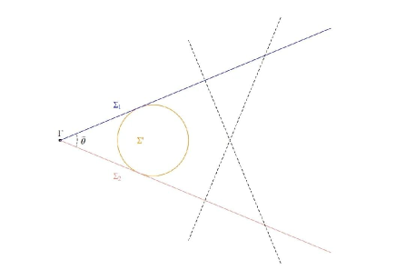
Figure 1: The $\Sigma_{1}$ and $\Sigma_{2}$ are the co-dimension one boundary surfaces. The $\tilde{\theta}$ is the interior angle between two surfaces, $\Sigma_{1}$ and $\Sigma_{2}$. The $\Gamma=\Sigma_{1}\cap\Sigma_{2}$ is the co-dimension two wedge term. The $\Sigma^{\prime}$ is a smooth 2d surface.

Note that we take

$$r=\epsilon,$$ (91)

and eventually, we would shrink $\epsilon$ to zero. Now we are only considering a thin slice of the joint. Therefore, one can always assume that the metric is locally flat around the joint. Therefore, the boundary condition at $r=\epsilon$ becomes:

$$(A_{t}-A_{\theta})|_{r=\epsilon\rightarrow 0}=0;\qquad(\bar{A}_{t}+\bar{A}_{\theta})|_{r=\epsilon\rightarrow 0}=0.$$ (92)

One can solve the wedge term by the boundary integration in the co-dimension one surface $\Sigma^{\prime}$ under the limit

$$\Sigma^{\prime}\to\Gamma$$ (93)

that collapses into integration in the co-dimension two joint [21].

We introduce the boundary term

$$S_{HCS}\equiv-\frac{k}{4\pi}\int_{\Sigma^{\prime}}dtd\theta\ \mathrm{Tr}(A_{\theta}^{2})-\frac{k}{4\pi}\int_{\Sigma^{\prime}}dtd\theta\ \mathrm{Tr}(\bar{A}_{\theta}^{2})$$ (94)

at

$$r=\epsilon,$$ (95)

instead of at infinity. The solutions of the gauge fields at the boundary are:

$$A=J_{0}dx^{+}+J_{2}dr;\qquad\bar{A}=\bar{J}_{0}dx^{-}+\bar{J}_{2}dr.$$ (96)

These solutions provide the following relation:

$$g^{-1}\partial_{\theta}g|_{r=0}$$ (97)

$$= \begin{pmatrix}\frac{1}{\lambda}\partial_{\theta}\lambda-\Psi\lambda^{2}\partial_{\theta}F&\partial_{\theta}\Psi+2\frac{\Psi}{\lambda}\partial_{\theta}\lambda-\Psi^{2}\lambda^{2}\partial_{\theta}F\\ \lambda^{2}\partial_{\theta}F&\lambda^{2}\Psi\partial_{\theta}F-\frac{1}{\lambda}\partial_{\theta}\lambda\end{pmatrix}\bigg{|}_{r=0}$$

$$= A_{\theta}|_{r=0}$$

$$= \begin{pmatrix}0&-\frac{1}{2}\\ \frac{1}{2}&0\end{pmatrix}.$$

This equality shows the following conditions:

$$\frac{1}{\lambda}\partial_{\theta}\lambda = \Psi\lambda^{2}\partial_{\theta}F;$$

$$\lambda^{2}\partial_{\theta}F = \frac{1}{2};$$

$$\partial_{\theta}\Psi+2\frac{\Psi}{\lambda}\partial_{\theta}\lambda-\Psi^{2}\lambda^{2}\partial_{\theta}F = -\frac{1}{2}.$$ (98)

Hence the conditions imply the following equations:

$$\lambda^{2}=\frac{1}{2\partial_{\theta}F};\qquad\frac{2}{\lambda}\partial_{\theta}\lambda=\Psi;\qquad\partial_{\theta}\Psi+\frac{1}{2}\Psi^{2}=-\frac{1}{2}.$$ (99)

After we substitute the boundary conditions to the bulk theory with the boundary term, we obtain the 2d Schwarzian theory for the $F$. For the $\bar{F}$, the result is similar. Hence combining the bulk theory and the boundary term gives

$$S_{BH}$$

$$= \frac{k}{2\pi}\int dtd\theta\ \bigg{(}\frac{3}{2}\frac{\partial_{-}\partial_{\theta}F\partial_{\theta}^{2}F}{(\partial_{\theta}F)^{2}}-\frac{\partial_{-}\partial_{\theta}^{2}F}{\partial_{\theta}F}\bigg{)}$$

$$-\frac{k}{2\pi}\int dtd\theta\ \bigg{(}\frac{3}{2}\frac{\partial_{+}\partial_{\theta}\bar{F}\partial_{\theta}^{2}\bar{F}}{(\partial_{\theta}\bar{F})^{2}}-\frac{\partial_{+}\partial_{\theta}^{2}\bar{F}}{\partial_{\theta}\bar{F}}\bigg{)}.$$

However, substituting the classical solution to the bulk term and Hayward term shows that only the boundary term survives. In the end, we obtain:

$$S_{BH}=-\frac{k}{2\pi}\int dtd\theta\ \mathrm{Tr}(e_{\theta}^{2}+\omega_{\theta}^{2})=\frac{1}{2}S_{H}.$$ (101)

The boundary term does not lead to the correct wedge term [27]. One can trace it back to the fact that the usual boundary term (94), when recast in the gauge formulation, is already off by a factor of two.

A way to fix this problem at the classical level is to consider double wedges. The setup is in Fig. 2.

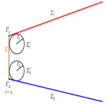
Figure 2: A construction with double wedges. The $\Sigma_{1}$ and $\Sigma_{2}$ are the co-dimension one boundary surfaces. The $\Sigma$ is a cut-off surface at $r=\epsilon$. We replace the two joints $\Gamma_{1}$ and $\Gamma_{2}$ with two caps of radius $r_{1}$ and $r_{2}$, respectively.

In this scenario, we impose co-dimension one surfaces $\Sigma_{1}$ and $\Sigma_{2}$ with the boundary condition (92). However, an additional cut-off surface is at

$$r=\epsilon.$$ (102)

We immediately see that this would introduce two cusp-like co-dimension two wedges. Following a similar procedure, we replace the two joints $\Gamma_{1}$ and $\Gamma_{2}$ with the two caps of the radius $r_{1}$ and $r_{2}$ respectively. We take two limits in the following order. We first shrink the two caps to zero radius to obtain the correct Hayward term. Eventually, we take the cut-off surface

$$\epsilon\to 0.$$ (103)

This limit provides a natural interpretation for considering a classical gravity dual of a CFT on a single interval. The two approaches differ in the order of the limits.

Classically, we have recovered the Hayward term. A natural question is whether one can use the wedge picture to construct the $n$-sheet manifold and perform a well-defined analytic continuation of $n\to 1$ in the quantum regime. We solve the fluctuation field in the equations of motion. Note that the equations of motion of the fluctuation field $F$ are:

$$\lambda^{2}=\frac{1}{2\partial_{\theta}F};\qquad\frac{2}{\lambda}\partial_{\theta}\lambda=\Psi;\qquad\partial_{\theta}\Psi+\frac{1}{2}\Psi^{2}=-\frac{1}{2}.$$ (104)

We can rewrite the equations as the following

$$\partial^{2}_{\theta}(\ln\partial_{\theta}F)-\frac{1}{2}(\partial_{\theta}(\ln\partial_{\theta}F))^{2}=\frac{1}{2}.$$ (105)

It is easy to obtain the general solution by:

$$f\equiv\ln\partial_{\theta}F=-2\ln\cos{\bigg{(}\frac{\theta}{2}+c_{1}(t)\bigg{)}}+c_{2}(t),$$ (106)

where $c_{1}(t)$ and $c_{2}(t)$ are arbitrary time-dependent functions. By doing the integration for $\theta$, we obtain the solution of the $F(\theta)$ as

$$F(\theta)=2\exp\big{(}c_{2}(t)\big{)}\tan{\bigg{(}\frac{\theta}{2}+c_{1}(t)\bigg{)}}+c_{3}(t),$$ (107)

where $c_{3}(t)$ is also an arbitrary time-dependent function. The solution is periodic for $\theta$

$$F(\theta)=F(\theta+2\pi).$$ (108)

When $\epsilon\rightarrow 0$, the wedge sits at the location of the AdS₃ minimum surface. In Fig. 3, we show the location of wedges compared to the minimum surface. Therefore, we can find how the minimum surface is generated from the wedges. The wedge method can provide boundary entanglement entropy.

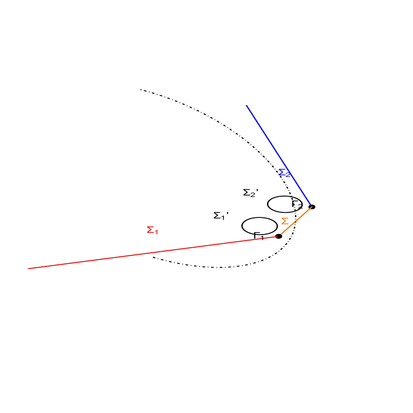
Figure 3: The dotted line is the AdS₃ minimum surface. The wedges are $\Gamma_{1}$ and $\Gamma_{2}$. When $r_{1},r_{2}=\epsilon\rightarrow 0$, two wedges approach to the minimum surface. The $\Sigma_{1}^{\prime}$ and $\Sigma_{2}^{\prime}$ are the co-dimension one cut-off surfaces. The $\Sigma$ is a cut-off surface at $r=\epsilon$.

We will discuss the result of the quantum contribution in the next section.

4 Entanglement Entropy at One-Loop

We calculate entanglement entropy for a single interval (with the length $L$) in the boundary theory of the SL(2) CS formulation [15]. For the convenience of calculation, we choose another form of the boundary theory on a spherical manifold [18]. Note that the calculation on the torus manifold is one-loop exact [18]. Therefore, the entanglement entropy is also one-loop exact. The entanglement entropy shows a shift of central charge, 26 [15], and the shifting does not appear in the U(1) case. In the end, we discuss the quantum correction for the Hayward approach [21]. The result shows that the quantum correction vanishes. Therefore, we have seen the difference between the approaches of the Wilson line [19] and Hayward terms [22] in the quantum regime. The details of Rényi entropy for the one-loop correction are in Appendix A.

4.1 Boundary Theory

After we integrate out $A_{t}$ and $\bar{A}_{t}$, the theory shows the form of the SL(2) transformations

$$S_{\mathrm{G}1}$$ (109)

$$= -\frac{k}{4\pi}$$

$$\times\int d^{3}x\ \mathrm{Tr}\bigg{(}-g^{-1}\big{(}\partial_{r}g\big{)}g^{-1}\big{(}\partial_{t}g\big{)}g^{-1}\partial_{\theta}g+g^{-1}\big{(}\partial_{r}g\big{)}g^{-1}\big{(}\partial_{\theta}g\big{)}g^{-1}\big{(}\partial_{t}g\big{)}\bigg{)}$$

$$+\frac{k}{4\pi}$$

$$\times\int d^{3}x\ \mathrm{Tr}\bigg{(}-\bar{g}^{-1}\big{(}\partial_{r}\bar{g}\big{)}\bar{g}^{-1}\big{(}\partial_{t}\bar{g}\big{)}\bar{g}^{-1}\partial_{\theta}\bar{g}+\bar{g}^{-1}\big{(}\partial_{r}\bar{g}\big{)}\bar{g}^{-1}\big{(}\partial_{\theta}\bar{g}\big{)}\bar{g}^{-1}\big{(}\partial_{t}\bar{g}\big{)}\bigg{)}$$

$$+\frac{k}{2\pi}\int dtd\theta\ \mathrm{Tr}\bigg{(}g^{-1}\big{(}\partial_{\theta}g\big{)}g^{-1}\big{(}D_{-}g\big{)}\bigg{)}$$

$$-\frac{k}{2\pi}\int dtd\theta\ \mathrm{Tr}\bigg{(}\bar{g}^{-1}\big{(}\partial_{\theta}\bar{g}\big{)}\bar{g}^{-1}\big{(}D_{+}\bar{g}\big{)}\bigg{)}.$$

By rewriting the SL(2) transformations in terms of other parameters, the effective action becomes:

$$S_{\mathrm{G}1}$$ (110)

$$= \frac{k}{\pi}\int dtd\theta\ \bigg{(}\frac{(\partial_{\theta}\lambda)(D_{-}\lambda)}{\lambda^{2}}+\lambda^{2}(\partial_{\theta}F)(D_{-}\Psi)\bigg{)}$$

$$-\frac{k}{\pi}\int dtd\theta\ \bigg{(}\frac{(\partial_{\theta}\bar{\lambda})(D_{+}\bar{\lambda})}{\bar{\lambda}^{2}}+\bar{\lambda}^{2}(\partial_{\theta}\bar{F})(D_{+}\bar{\Psi})\bigg{)}.$$

Due to the following boundary conditions:

$$\lambda^{2}\partial_{\theta}F=E_{\theta}^{+}r;\qquad\bar{\lambda}^{2}\partial_{\theta}\bar{F}=E_{\theta}^{-}r,$$ (111)

the following terms:

$$\frac{k}{\pi}\int dtd\theta\ \bigg{(}\lambda^{2}(\partial_{\theta}F)(D_{-}\Psi)\bigg{)},\qquad-\frac{k}{\pi}\int dtd\theta\ \bigg{(}\bar{\lambda}^{2}(\partial_{\theta}\bar{F})(D_{+}\bar{\Psi})\bigg{)}$$ (112)

are total derivative terms. Therefore, the boundary effective action becomes

$$S_{\mathrm{G}1}=\frac{k}{\pi}\int dtd\theta\ \bigg{(}\frac{(\partial_{\theta}\lambda)(D_{-}\lambda)}{\lambda^{2}}-\frac{(\partial_{\theta}\bar{\lambda})(D_{+}\bar{\lambda})}{\bar{\lambda}^{2}}\bigg{)}.$$ (113)

With the definition:

$${\cal F}\equiv\frac{F}{E^{+}_{\theta}};\qquad\bar{{\cal F}}\equiv\frac{\bar{F}}{E_{\theta}^{-}},$$ (114)

we obtain:

$$\lambda=\sqrt{\frac{r}{\partial_{\theta}{\cal F}}};\qquad\bar{\lambda}=\sqrt{\frac{r}{\partial_{\theta}\bar{{\cal F}}}}.$$ (115)

Therefore, we obtain the boundary action

$$S_{\mathrm{G}1}=\frac{k}{4\pi}\int dtd\theta\ \bigg{(}\frac{(\partial_{\theta}^{2}{\cal F})(D_{-}\partial_{\theta}{\cal{F}})}{(\partial_{\theta}{\cal F})^{2}}-\frac{(\partial_{\theta}^{2}\bar{{\cal F}})(D_{+}\partial_{\theta}\bar{{\cal{F}}})}{(\partial_{\theta}\bar{{\cal F}})^{2}}\bigg{)}.$$ (116)

Finally, we choose the field redefinition:

$${\cal F}\equiv\tan\bigg{(}\frac{\phi}{2}\bigg{)};\qquad\bar{{\cal F}}\equiv\tan\bigg{(}\frac{\bar{\phi}}{2}\bigg{)}$$ (117)

to obtain

$$S_{\mathrm{G}1}$$ (118)

$$= \frac{k}{4\pi}\int dtd\theta\ \bigg{[}\frac{(\partial_{\theta}^{2}\phi)(D_{-}\partial_{\theta}\phi)}{(\partial_{\theta}\phi)^{2}}-(\partial_{\theta}\phi)(D_{-}\phi)\bigg{]}$$

$$-\frac{k}{4\pi}\int dtd\theta\ \bigg{[}\frac{(\partial_{\theta}^{2}\bar{\phi})(D_{+}\partial_{\theta}\bar{\phi})}{(\partial_{\theta}\bar{\phi})^{2}}-(\partial_{\theta}\bar{\phi})(D_{+}\bar{\phi})\bigg{]},$$

up to a total derivative term.

4.2 Spherical Manifold

Using Weyl transformations, the Euclidean AdS₃ metric approaching to a boundary ($r\rightarrow\infty$) can be written as [10]

$$ds^{2}=\frac{dr^{2}}{r^{2}}+r^{2}ds_{s}^{2},$$ (119)

where

$$ds_{s}^{2}\equiv d\psi^{2}+\sin^{2}\psi d\theta^{2},\ 0\leq\psi<\pi,\ 0\leq\theta<2\pi.$$ (120)

The boundary zweibein is:

$$E_{\theta}^{+}=E_{\theta}^{-}=\sin\psi;\qquad E_{\psi}^{+}=-iE_{t}^{+}=i;\qquad E_{\psi}^{-}=-iE_{t}^{-}=-i.$$ (121)

4.3 Entanglement Entropy for Single Interval

To calculate entanglement entropy for a single interval, we first identify the boundary conditions of fields. We then calculate entanglement entropy and compare the result to the U(1) case. We calculate the Rényi entropy

$$S_{n}\equiv\frac{\ln Z_{n}-n\ln Z_{1}}{1-n}$$ (122)

from the replica trick [8], where $Z_{n}$ is the $n$-sheet partition function, and $Z_{1}$ is equivalent to the partition function. When $n\rightarrow 1$, the Rényi entropy gives entanglement entropy. The calculation is one-loop exact. Therefore, the quantum fluctuation of the $n$-sheet partition function only comes from the one-loop order. We then obtain that the $n$-sheet partition function is a product of the classical $n$-sheet partition-function ($Z_{n,c}$) and the one-loop $n$-sheet partition-function ($Z_{n,q}$)

$$Z_{n}=Z_{n,c}\cdot Z_{n,q}.$$ (123)

Calculating the Rényi entropy is necessary to take the logarithm on the $n$-sheet partition function

$$\ln Z_{n}=\ln Z_{n,c}+\ln Z_{n,q}.$$ (124)

Hence the contribution from the classical and the one-loop terms is not mixed.

4.3.1 $n$-Sheet Manifold

We first do a coordinate transformation on the unit sphere $ds_{s}^{2}$ to obtain

$$ds_{s}^{2}=\operatorname{sech}^{2}(y)(dy^{2}+d\theta^{2}),$$ (125)

where

$$\operatorname{sech}y\equiv\sin\psi.$$ (126)

The range of $\theta$ in the $n$-sheet manifold becomes

$$0<\theta\leq 2\pi n.$$ (127)

The periodicity of $\theta$ becomes $2\pi n$ now. The $y$-direction needs regularization, and the range becomes

$$-\ln\frac{L}{\epsilon}<y\leq\ln\frac{L}{\epsilon},$$ (128)

where $\epsilon$ is a cut-off. We sum two momentum modes with different boundary conditions. One mode satisfies the Dirichlet boundary condition in the $y$-direction. Another one follows the Neumann boundary conditions. Therefore, the periodicity is $4\ln(L/\epsilon)$.

4.3.2 Boundary Condition

Now we map the sphere to the torus. We choose the coordinates of an $n$-sheet torus

$$z\equiv\frac{\theta+iy}{n}$$ (129)

with the identification:

$$z\sim z+2\pi;\qquad z\sim z+2\pi\tau_{n}.$$ (130)

The identification leads to the boundary condition [15]:

$$\phi\bigg{(}\frac{y}{n},\frac{\theta}{n}+2\pi\bigg{)} = \phi\bigg{(}\frac{y}{n},\frac{\theta}{n}\bigg{)}+2\pi;$$

$$\phi\bigg{(}\frac{y}{n}+2\pi\cdot\mathrm{Im}(\tau_{n}),\frac{\theta}{n}+2\pi\cdot\mathrm{Re}(\tau_{n})\bigg{)} = \phi\bigg{(}\frac{y}{n},\frac{\theta}{n}\bigg{)},$$

$$\bar{\phi}\bigg{(}\frac{y}{n},\frac{\theta}{n}+2\pi\bigg{)} = \bar{\phi}\bigg{(}\frac{y}{n},\frac{\theta}{n}\bigg{)}+2\pi;$$

$$\bar{\phi}\bigg{(}\frac{y}{n}+2\pi\cdot\mathrm{Im}(\tau_{n}),\frac{\theta}{n}+2\pi\cdot\mathrm{Re}(\tau_{n})\bigg{)} = \bar{\phi}\bigg{(}\frac{y}{n},\frac{\theta}{n}\bigg{)}.$$ (131)

Due to the periodicity of $y$, the complex structure corresponds to the unit sphere is [15]

$$\tau_{n}=\bigg{(}\frac{2i}{n\pi}\bigg{)}\ln\bigg{(}\frac{L}{\epsilon}\bigg{)}.$$ (132)

Note that

$$\mathrm{Re}(\tau_{n})=0.$$ (133)

The Fourier transformation of the fields gives:

$$\phi=\frac{\theta}{n}+\epsilon(y,\theta);\qquad\bar{\phi}=-\frac{\theta}{n}+\bar{\epsilon}(y,\theta),$$ (134)

where

$$\epsilon(y,\theta) \equiv \sum_{j,k}\epsilon_{j,k}e^{i\frac{j}{n}\theta-\frac{k}{\tau}y};\qquad\epsilon_{j,k}^{*}\equiv\epsilon_{-j,-k},$$

$$\bar{\epsilon}(y,\theta) \equiv \sum_{j,k}\bar{\epsilon}_{j,k}e^{i\frac{j}{n}\theta-\frac{k}{\tau}y};\qquad\bar{\epsilon}_{j,k}^{*}\equiv\bar{\epsilon}_{-j,-k}.$$ (135)

The saddle-point is the $\theta/n$ in the $\phi$ and the $-\theta/n$ in the $\bar{\phi}$. Each Fourier mode has three zero-modes:

$$\epsilon_{j,k}=0;\qquad\bar{\epsilon}_{j,k}=0,\ j=-1,0,1$$ (136)

because of the SL(2) gauge symmetry.

4.3.3 Entanglement Entropy

To calculate the $n$-sheet partition function, we need to Wick rotate for the boundary effective action:

$$S_{\mathrm{EG}1}$$

$$= -\frac{k}{4\pi}\int_{0}^{\pi}d\psi\int_{0}^{2\pi n}d\theta\ \bigg{[}\frac{(\partial_{\theta}^{2}\phi)(D_{-}\partial_{\theta}\phi)}{(\partial_{\theta}\phi)^{2}}-(\partial_{\theta}\phi)(D_{-}\phi)\bigg{]}$$

$$+\frac{k}{4\pi}\int_{0}^{\pi}d\psi\int_{0}^{2\pi n}d\theta\ \bigg{[}\frac{(\partial_{\theta}^{2}\bar{\phi})(D_{+}\partial_{\theta}\bar{\phi})}{(\partial_{\theta}\bar{\phi})^{2}}-(\partial_{\theta}\bar{\phi})(D_{+}\bar{\phi})\bigg{]}$$

$$= \frac{k}{4\pi}\int_{-\frac{\pi}{2}\mathrm{Im}(\tau)}^{\frac{\pi}{2}\mathrm{Im}(\tau)}dy\int_{0}^{2\pi n}d\theta\ \operatorname{sech}(y)\bigg{[}\frac{(\partial_{\theta}^{2}\phi)(D_{-}\partial_{\theta}\phi)}{(\partial_{\theta}\phi)^{2}}-(\partial_{\theta}\phi)(D_{-}\phi)\bigg{]}$$

$$-\frac{k}{4\pi}\int_{-\frac{\pi}{2}\mathrm{Im}(\tau)}^{\frac{\pi}{2}\mathrm{Im}(\tau)}dy\int_{0}^{2\pi n}d\theta\ \operatorname{sech}(y)\bigg{[}\frac{(\partial_{\theta}^{2}\bar{\phi})(D_{+}\partial_{\theta}\bar{\phi})}{(\partial_{\theta}\bar{\phi})^{2}}-(\partial_{\theta}\bar{\phi})(D_{+}\bar{\phi})\bigg{]},$$

in which the covariant derivative becomes:

$$D_{+} = \frac{i}{2}\partial_{\psi}-\frac{i}{2}\frac{E_{\psi}^{-}}{E_{\theta}^{-}}\partial_{\theta}=\frac{i}{2}\partial_{\psi}-\frac{1}{2\sin\psi}\partial_{\theta}=-\frac{i}{2}\cosh(y)\partial_{y}-\frac{1}{2}\cosh(y)\partial_{\theta},$$

$$D_{-} = \frac{i}{2}\partial_{\psi}-\frac{i}{2}\frac{E_{\psi}^{+}}{E_{\theta}^{+}}\partial_{\theta}=\frac{i}{2}\partial_{\psi}+\frac{1}{2\sin\psi}\partial_{\theta}=-\frac{i}{2}\cosh(y)\partial_{y}+\frac{1}{2}\cosh(y)\partial_{\theta}.$$

We substitute the saddle-point into the boundary effective action and note that

$$c=6k$$ (139)

as the central charge of CFT₂, we have:

$$-\frac{k}{4\pi}\int_{-\frac{\pi}{2}\mathrm{Im}(\tau)}^{\frac{\pi}{2}\mathrm{Im}(\tau)}dy\int_{0}^{2\pi n}d\theta\ \frac{1}{2n^{2}}-\frac{k}{4\pi}\int_{-\frac{\pi}{2}\mathrm{Im}(\tau)}^{\frac{\pi}{2}\mathrm{Im}(\tau)}dy\int_{0}^{2\pi n}d\theta\ \frac{1}{2n^{2}}$$ (140)

$$= \frac{-c\pi\tau}{12n}$$

$$= -\frac{c}{6n}\ln\frac{L}{\epsilon},$$

where

$$\tau\equiv n\tau_{n}.$$ (141)

Therefore, we obtain

$$\ln Z_{n,c}=\frac{c}{6n}\ln\frac{L}{\epsilon}.$$ (142)

The Rényi entropy from the saddle-point is:

$$S_{n,c}=\frac{c}{1-n}\bigg{(}\frac{1}{6n}-\frac{n}{6}\bigg{)}\ln\frac{L}{\epsilon}=\frac{c(1+n)}{6n}\ln\frac{L}{\epsilon}.$$ (143)

When we take $n\rightarrow 1$, the saddle-point contributes to the entanglement entropy

$$S_{1,c}=\frac{c}{3}\ln\frac{L}{\epsilon}.$$ (144)

The Rényi entropy from the one-loop correction is given by:

$$S_{n,q}=\frac{1}{1-n}\big{(}\ln Z_{n,q}-n\ln Z_{1,q}\big{)}=\frac{13(n+1)}{3n}\ln\frac{L}{\epsilon}.$$ (145)

Therefore, the summation of classical and one-loop terms gives the Rényi entropy

$$S_{n}=\frac{(c+26)(n+1)}{6n}\ln\frac{L}{\epsilon}$$ (146)

and the entanglement entropy

$$S_{1}=\frac{c+26}{3}\ln\frac{L}{\epsilon}.$$ (147)

The details of the one-loop correction are in Appendix A.

The result shows that the quantum contribution does not change the form of Rényi entropy and entanglement entropy. It shifts the value of the central charge by 26. Hence the conformal anomaly does not take the Rényi entropy and entanglement entropy to go beyond the results of CFT₂. For the U(1) case, entanglement entropy does not have such a shift from the $k^{0}$ term, and it is proportional to $k$. The difference between the U(1) and SL(2) cases is self-interaction. Therefore, the interaction vanishes in the weak gravitational constant limit $k\rightarrow\infty$. Hence the shift of the central charge or the one-loop contribution is due to the self-interaction. This result shows that the SL(2) CS formulation should match the U(1) CS theory in the weak gravitational constant limit.

The U(1) theory only has two degrees of freedom, but the SL(2) formulation has six. It interprets why the geometry can be related to the SL(2) formulation but not the U(1) theory. However, their equivalence is on the boundary. The bulk does not have dynamical degrees of freedom. The asymptotic gauge fields showing the AdS₃ metric give the additional four required constraints. Its boundary theory provides consistent degrees with the U(1) case. The self-interaction term indicates the difference between the U(1) and SL(2) cases. However, it does not affect the physical degrees of freedom. Hence studying the exact solution in the U(1) case provides a better understanding of the SL(2) case.

4.4 Hayward Term

We discuss whether it is possible to study the quantum correction by computing the bulk and Hayward terms. From the solution (107), we choose the saddle point as in the Wilson line:

$$F_{saddle}\equiv 2\exp\big{(}c_{2}(t)\big{)}\tan\bigg{(}\frac{\theta}{2}\bigg{)}+c_{3}(t).$$ (148)

By substituting the solution into the action with the field redefinition (117), the $c_{2}(t)$ and $c_{3}(t)$ would not affect the result. Because the introduction of the $n$-sheet torus with the boundary conditions for the $\phi$ would be the same, the quantum fluctuation only comes from the $c_{1}(t)$ term in Eq. (107). All situations are similar to the Wilson line, except that the quantum fluctuation does not depend on the $\theta$. The non-vanishing one-loop result relies on the non-trivial dependence of the $\theta$. Therefore, the partition function does not include quantum fluctuation. Introducing the $n$-sheet manifold to the approach of the Hayward term [22], the quantum fluctuation still cannot generate the dependence of the $\theta$. Therefore, the result implies the inconsistency between the entanglement entropy and naive quantum generalization to the quantum regime. This fact shows why the classical term is too universal, and including quantum contribution is a non-trivial task.

5 Discussion and Conclusion

In this paper, we studied holographic entanglement entropy [6]. We considered the SL(2) CS formulation [13] for the AdS₃ Einstein gravity theory and compared it to the U(1) CS theory. We then showed that the Wilson line is a suitable bulk operator for obtaining entanglement entropy of the boundary theory [15, 19, 20]. This proof is quite non-trivial because it is non-perturbative. We also showed that the Hayward term [21] in the SL(2) CS formulation reproduces the entanglement entropy at the classical level by a double-wedges construction. Combining the bulk and Hayward terms for a quantum generalization provides the vanishing quantum correction in the partition function. Hence the Wilson line is a suitable candidate for studying entanglement entropy. The proof strengthens the correspondence of “minimum surface=entanglement entropy”, but it relies on a smooth limit of the analytical continuation [15]. Hence it is not clear why such equivalence can appear. This result motivates us to find a simple system to do a similar exact study. We can study the Wilson line in the U(1) CS theory to establish the equivalence. The equivalence is necessary to deform the boundary after the back-reaction of the Wilson line. The chiral scalar fields are not relevant to geometry (in the U(1) CS theory). Therefore, the deformation of boundary conditions and back-reaction cannot appear simultaneously. However, it does not imply that the boundary fields can reconstruct kinematic information (boundary geometry) in the U(1) CS theory. It is mainly because the numbers of gauge fields on the bulk are not equivalent. The weak gravitational constant limit does not play a role in defining geometry. In the SL(2) CS formulation, the back-reaction deforms the gauge fields and also the geometry [19, 20]. Because the boundary zweibein is coupled to the boundary gauge fields, deforming the geometry is equivalent to changing the boundary condition and theory. We calculated entanglement entropy in the SL(2) CS formulation. The result showed a shift of the central charge by 26 [15]. Therefore, the shift should be due to the self-interaction term (because the U(1) case loses it).

The U(1) CS theory has two independent gauge fields, but the SL(2) CS formulation has six gauge fields. It seems that their physical degrees of freedom do not match. However, the bulk theory in a topological theory does not have dynamics. We need to compare the physical degrees of freedom in the boundary theories. In the SL(2) CS formulation, the AdS₃ geometry constrains the asymptotic gauge fields. The constraint leads the boundary theory to have the equivalent physical degrees of freedom to the U(1) CS theory. The SL(2) CS formulation has one self-interacting term in the boundary theory. The term does not appear in the U(1) case. However, the local interacting term does not change the physical degrees of freedom. Because the interacting term vanishes in the weak gravitational constant limit, the pure AdS₃ Einstein gravity theory approaches the U(1) CS theory. The reduction itself is not trivial. The various exact results also complement the SL(2) CS formulation.

We comment on the holographic principle in the SL(2) CS formulation. For obtaining entanglement entropy, the bulk calculation reduces to the boundary calculation. The study provides a better understanding of the holographic principle. The classical contribution is usually not enough to justify different proposals or conjectures. The holographic principle works here because it requires one necessary condition, the coupling between boundary fields and the asymptotic metric field. By studying the U(1) CS theory, we know that the condition is not trivial. In this case, changing the boundary condition (or Lagrangian) after introducing the geodesic operator (Wilson lines) is necessary.

In the end, we discuss other local AdS spaces. In general other locally AdS spaces like BTZ black hole can be obtained from pure AdS by a quotient of some discrete subgroup $\Gamma$ of the isometry group PSL$(2,\mathbb{C})$. The correspondence between pure Einstein gravity and the Schwarzian theory on the boundary remains valid in any event. In this sense, we expect that our computation of quantum correction can be generalized to other backgrounds like AdS black holes. We have Riemann surfaces of higher genus after the replica trick. Explicit computation by solving eigenvalues is beyond the scope of the current manuscript. One can obtain the form of the one-loop correction from earlier results. It is well-known that the one-loop contribution from the Schwarzian theory agrees with the bulk one-loop partition function of graviton [18]. In a general background $\mathbb{H}^{3}/\Gamma$, the bulk one-loop partition function can be obtained as a product form [14]

$$Z^{\mathbb{H}^{3}/\Gamma}=\prod_{\gamma\in{\cal P}}Z^{\mathbb{H}^{3}/\langle\gamma\rangle},$$ (149)

where the product is over the primitive conjugate classes of $\Gamma$. Each $Z^{\mathbb{H}^{3}/\langle\gamma\rangle}$ is the one-loop partition on a solid torus and hence agrees with our one-loop contribution (it follows from the boundary Schwarzian theory on a torus). It is natural to expect that the one-loop contribution from the boundary Schwarzian theory always agrees with that of the bulk graviton. Hence the quantum correction given by Eq. (149) on the right-hand side is explicitly known.

Appendix A Details of Rényi Entropy for One-Loop

Now we consider the quantum fluctuation from the $\epsilon(y,\theta)$ and $\bar{\epsilon}(y,\theta)$ to obtain the one-loop term [15]. Because the contributions from the sector of $\phi$ and $\bar{\phi}$ are the same, we only show the calculation related to the $\phi$ field. The expansion from the $\epsilon$ in the boundary effective action is [15]

$$\frac{k}{4\pi}\int_{-\frac{\pi}{2}\mathrm{Im}(\tau)}^{\frac{\pi}{2}\mathrm{Im}(\tau)}dy\int_{0}^{2\pi n}d\theta\ \bigg{(}n^{2}\big{(}\partial_{\theta}^{2}\epsilon(y,\theta)\big{)}\big{(}\bar{\partial}\partial_{\theta}\epsilon(y,\theta)\big{)}$$ (150)

$$-\big{(}\partial_{\theta}\epsilon(y,\theta)\big{)}\big{(}\bar{\partial}\epsilon(y,\theta)\big{)}\bigg{)}$$

$$= -i\frac{k}{4\pi}n\tau\cdot\bigg{\{}n^{2}\sum_{j,k}\bigg{[}\bigg{(}-\frac{j^{2}}{n^{2}}\cdot\frac{1}{2}\cdot\bigg{(}i\frac{k}{\tau}+i\frac{j}{n}\bigg{)}\bigg{(}i\frac{j}{n}\bigg{)}\bigg{]}|\epsilon_{j,k}|^{2}$$

$$-\sum_{j,k}\bigg{[}\bigg{(}i\frac{j}{n}\bigg{)}\cdot\frac{1}{2}\cdot\bigg{(}i\frac{k}{\tau}+i\frac{j}{n}\bigg{)}\bigg{]}|\epsilon_{j,k}|^{2}\bigg{\}}$$

$$= -i\frac{k}{8\pi}\sum_{j,k}j(j^{2}-1)\bigg{(}k+\frac{j}{n}\tau\bigg{)}|\epsilon_{j,k}|^{2},$$

where

$$\bar{\partial}\equiv\frac{1}{2}(-i\partial_{y}+\partial_{\theta}).$$ (151)

Doing the derivative on the logarithm of the $n$-sheet one-loop partition shows

$$\partial_{\tau}\ln Z_{n,q}=-\sum_{j\neq 0,\pm 1}\sum_{k=-\infty}^{\infty}\frac{\frac{j}{n}}{k+\frac{j}{n}\tau}.$$ (152)

Applying the following useful relation of the digamma function, we obtain

$$\tilde{\psi}(1-x)-\tilde{\psi}(x)=\pi\cot(\pi x),$$ (153)

in which the digamma function is defined by

$$\tilde{\psi}(a)\equiv-\sum_{n=0}^{\infty}\frac{1}{n+a}.$$ (154)

Therefore, the complicated summation in the $n$-sheet partition function simplified as:

$$\sum_{m=-\infty}^{\infty}\frac{1}{m-x} = -\sum_{m=0}^{\infty}\frac{1}{m+x}+\sum_{m=1}^{\infty}\frac{1}{m-x}$$ (155)

$$= -\sum_{m=0}^{\infty}\frac{1}{m+x}+\sum_{m=0}^{\infty}\frac{1}{m+1-x}=\tilde{\psi}(x)-\tilde{\psi}(1-x)$$

$$= -\pi\cdot\cot(\pi x).$$

Hence we obtain:

$$\partial_{\tau}\ln Z_{n,q} = -\sum_{j\neq 0,\pm 1}\sum_{k=-\infty}^{\infty}\frac{\frac{j}{n}}{k+\frac{j}{n}\tau}=-\sum_{j\neq 0,\pm 1}\bigg{(}\frac{j}{n}\pi\bigg{)}\cdot\cot\bigg{(}\frac{j}{n}\pi\tau\bigg{)}$$ (156)

$$= -2\pi\sum_{j=2}^{\infty}\bigg{(}\frac{j}{n}\bigg{)}\cdot\cot\bigg{(}\frac{j\pi\tau}{n}\bigg{)}.$$

To obtain a universal term, we use the re-summation:

$$\partial_{\tau}\ln Z_{n,q} = -2\pi\sum_{j=2}^{\infty}\bigg{(}\frac{j}{n}\bigg{)}\cdot\cot\bigg{(}\frac{j\pi\tau}{n}\bigg{)}$$

$$= -2\pi\sum_{j=2}^{\infty}\frac{j}{n}\cdot\bigg{[}\cot\bigg{(}\frac{j\pi\tau}{n}\bigg{)}+i\bigg{]}+2\pi i\sum_{j=2}^{\infty}\frac{j}{n}.$$

We can perform a regularization for the divergent series

$$\sum_{j=1}^{\infty}j\rightarrow-\frac{1}{12}.$$ (158)

Hence we obtain:

$$\partial_{\tau}\ln Z_{n,q} = -2\pi\sum_{j=2}^{\infty}\frac{j}{n}\cdot\bigg{[}\cot\bigg{(}\frac{j\pi\tau}{n}\bigg{)}+i\bigg{]}+2\pi i\sum_{j=2}^{\infty}\frac{j}{n}$$ (159)

$$\rightarrow -2\pi\sum_{j=2}^{\infty}\frac{j}{n}\cdot\bigg{[}\cot\bigg{(}\frac{j\pi\tau}{n}\bigg{)}+i\bigg{]}-i\frac{13\pi}{6n}.$$

After integrating out the $\tau$, we obtain

$$\ln Z_{n,q}=-2\sum_{j=2}^{\infty}\bigg{[}\ln\sin\bigg{(}\frac{\pi j\tau}{n}\bigg{)}+i\frac{j\pi\tau}{n}\bigg{]}-i\frac{13\pi\tau}{6n}+\cdots,$$ (160)

where $\cdots$ is independent of the $\tau$. The first series is convergent for the

$$\mathrm{Im}(\tau)>0.$$ (161)

When we consider the limit

$$\frac{L}{\epsilon}\rightarrow\infty,$$ (162)

we obtain

$$\ln Z_{n,q}=\frac{13}{3n}\ln\frac{L}{\epsilon},$$ (163)

and the Rényi entropy for the one-loop correction is [15]:

$$S_{n,q}=\frac{1}{1-n}\big{(}\ln Z_{n,q}-n\ln Z_{1,q}\big{)}=\frac{13(n+1)}{3n}\ln\frac{L}{\epsilon}.$$ (164)

References

- [1] J. D. Bekenstein, “Black holes and entropy,” Phys. Rev. D 7, 2333-2346 (1973) doi:10.1103/PhysRevD.7.2333
- [2] J. M. Bardeen, B. Carter and S. W. Hawking, “The Four laws of black hole mechanics,” Commun. Math. Phys. 31, 161-170 (1973) doi:10.1007/BF01645742
- [3] S. W. Hawking, “Particle Creation by Black Holes,” Commun. Math. Phys. 43, 199-220 (1975) doi:10.1007/BF02345020
- [4] G. ’t Hooft, “Dimensional reduction in quantum gravity,” Conf. Proc. C 930308, 284 (1993) [gr-qc/9310026].
- [5] L. Susskind, “The World as a hologram,” J. Math. Phys. 36, 6377-6396 (1995) doi:10.1063/1.531249 [arXiv:hep-th/9409089 [hep-th]].
- [6] S. Ryu and T. Takayanagi, “Holographic derivation of entanglement entropy from AdS/CFT,” Phys. Rev. Lett. 96, 181602 (2006) doi:10.1103/PhysRevLett.96.181602 [hep-th/0603001].
- [7] S. Ryu and T. Takayanagi, “Aspects of Holographic Entanglement Entropy,” JHEP 08, 045 (2006) doi:10.1088/1126-6708/2006/08/045 [arXiv:hep-th/0605073 [hep-th]].
- [8] C. Holzhey, F. Larsen and F. Wilczek, “Geometric and renormalized entropy in conformal field theory,” Nucl. Phys. B 424, 443 (1994) doi:10.1016/0550-3213(94)90402-2 [hep-th/9403108].
- [9] A. Lewkowycz and J. Maldacena, “Generalized gravitational entropy,” JHEP 1308, 090 (2013) doi:10.1007/JHEP08(2013)090 [arXiv:1304.4926 [hep-th]].
- [10] H. Casini, M. Huerta and R. C. Myers, “Towards a derivation of holographic entanglement entropy,” JHEP 05, 036 (2011) doi:10.1007/JHEP05(2011)036 [arXiv:1102.0440 [hep-th]].
- [11] S. Elitzur, G. W. Moore, A. Schwimmer and N. Seiberg, “Remarks on the Canonical Quantization of the Chern-Simons-Witten Theory,” Nucl. Phys. B 326, 108 (1989). doi:10.1016/0550-3213(89)90436-7
- [12] J. D. Brown and M. Henneaux, “Central Charges in the Canonical Realization of Asymptotic Symmetries: An Example from Three-Dimensional Gravity,” Commun. Math. Phys. 104, 207 (1986). doi:10.1007/BF01211590
- [13] E. Witten, “(2+1)-Dimensional Gravity as an Exactly Soluble System,” Nucl. Phys. B 311, 46 (1988). doi:10.1016/0550-3213(88)90143-5
- [14] S. Giombi, A. Maloney and X. Yin, “One-loop Partition Functions of 3D Gravity,” JHEP 08, 007 (2008) doi:10.1088/1126-6708/2008/08/007 [arXiv:0804.1773 [hep-th]].
- [15] X. Huang, C. T. Ma and H. Shu, “Quantum Correction of the Wilson Line and Entanglement Entropy in the Pure AdS3 Einstein Gravity Theory,” Phys. Lett. B 806, 135515 (2020) doi:10.1016/j.physletb.2020.135515 [arXiv:1911.03841 [hep-th]].
- [16] O. Coussaert, M. Henneaux and P. van Driel, “The Asymptotic dynamics of three-dimensional Einstein gravity with a negative cosmological constant,” Class. Quant. Grav. 12, 2961 (1995) doi:10.1088/0264-9381/12/12/012 [gr-qc/9506019].
- [17] E. Witten, “Three-Dimensional Gravity Revisited,” arXiv:0706.3359 [hep-th].
- [18] J. Cotler and K. Jensen, “A theory of reparameterizations for AdS3 gravity,” JHEP 1902, 079 (2019) doi:10.1007/JHEP02(2019)079 [arXiv:1808.03263 [hep-th]].
- [19] M. Ammon, A. Castro and N. Iqbal, “Wilson Lines and Entanglement Entropy in Higher Spin Gravity,” JHEP 1310, 110 (2013) doi:10.1007/JHEP10(2013)110 [arXiv:1306.4338 [hep-th]].
- [20] J. de Boer and J. I. Jottar, “Entanglement Entropy and Higher Spin Holography in AdS3,” JHEP 1404, 089 (2014) doi:10.1007/JHEP04(2014)089 [arXiv:1306.4347 [hep-th]].
- [21] G. Hayward, “Gravitational action for space-times with nonsmooth boundaries,” Phys. Rev. D 47, 3275-3280 (1993) doi:10.1103/PhysRevD.47.3275
- [22] T. Takayanagi and K. Tamaoka, “Gravity Edges Modes and Hayward Term,” JHEP 02, 167 (2020) doi:10.1007/JHEP02(2020)167 [arXiv:1912.01636 [hep-th]].
- [23] M. Botta-Cantcheff, P. J. Martinez and J. F. Zarate, “Rényi entropies and area operator from gravity with Hayward term,” JHEP 07, no.07, 227 (2020) doi:10.1007/JHEP07(2020)227 [arXiv:2005.11338 [hep-th]].
- [24] X. Dong, “The Gravity Dual of Renyi Entropy,” Nature Commun. 7, 12472 (2016) doi:10.1038/ncomms12472 [arXiv:1601.06788 [hep-th]].
- [25] R. Floreanini and R. Jackiw, “Selfdual Fields as Charge Density Solitons,” Phys. Rev. Lett. 59, 1873 (1987) doi:10.1103/PhysRevLett.59.1873
- [26] A. A. Tseytlin and P. C. West, “TWO REMARKS ON CHIRAL SCALARS,” Phys. Rev. Lett. 65, 541-542 (1990) doi:10.1103/PhysRevLett.65.541
- [27] M. Rooman and P. Spindel, “Holonomies, anomalies and the Fefferman-Graham ambiguity in AdS(3) gravity,” Nucl. Phys. B 594, 329-353 (2001) doi:10.1016/S0550-3213(00)00636-2 [arXiv:hep-th/0008147 [hep-th]].