Thick branes with inner structure in mimetic $f(R)$ gravity

Abstract

In this paper, we study the structure and gravitational resonances of thick branes generated by a mimetic scalar field in $f(R)$ gravity. We obtain several typical thick brane solutions for $f(R)=R+\alpha R^{2}$. To study their stability, we analyze the tensor perturbation of the metric. It is shown that any thick brane model with $df/dR>0$ is stable and the graviton zero mode can be localized on the brane for each solution, which indicates that the four-dimensional Newtonian gravity can be restored. The effect of the parameter $\alpha$ on the gravitational resonances is studied. As a brane splits into multi sub-branes, the effective potential of the tensor perturbation will have an abundant inner structure with multi-wells, and this will lead to new phenomena of the gravitational resonances.

I Introduction

In last twenty years, brane world scenario has been an attractive topic and researched widely. Arkani-Hamed, Dimopoulos, and Dvali (ADD) provided an alternative solution to gauge hierarchy problem Arkani-Hamed1998 . In ADD model, all matter fields are confined on a four-dimensional brane which is embedded in a higher-dimensional spacetime, only gravity can propagate in the bulk. After that, Randall and Sundrum proposed two different kinds of extra dimension models, RS-1 Randall1999a and RS-2 model Randall1999 . In RS-1 model the extra dimension is compact and warped but in RS-2 model the scale of the warped extra dimension is infinite. In RS-2 model, the four-dimensional Newtonian potential can be restored even if the scale of the extra dimension is infinite. However, the thicknesses of the brane of RS models are neglected, and this is the reason why we called them thin brane models. Combining the RS-2 model with the domain wall model Rubakov1983 one can generalize the RS-2 model to a thick brane model DeWolfe2000 ; Csaki2000 ; Gremm2000 . The localization problem of matter fields on a thick brane was studied in Refs. DeWolfe2000 ; Gremm2000 ; Kehagias2001 ; Melfo2006 ; Almeida2009 ; Zhao2010 ; Chumbes2011 ; Liu2011 ; Xie2017 ; Gu2017 ; ZhongYuan2017 ; ZhongYuan2017b ; Zhou2018 . In thick brane world scenario, the brane is usually generated by a canonical scalar field Liu2012 ; Xu2015 ; Yu2016 ; Cruz2019 ; Wan2020 ; Rosa2020 . Furthermore, various kinds of thick branes generated by multi-scalar fields were also investigated widely Bazeia2004 ; DeSouzaDutra2008 ; Dutra2015 ; ZhongYuan2018a ; Xie2020 . For more details of thick brane worlds and extra dimensions, see the review papers Dzhunushaliev0904.1775 ; Herrera-Aguilar0910.0363 ; Liu2018review .

On the other hand, physicists should answer what cause late-time universe acceleration and what is dark matter. To solve these issues indicated by astronomical observations, physicists provided two kinds of schemes, one is assuming the existence of extra energy and matter, the other one is modifying general relativity to match observations. Furthermore, renormalization of gravity is another motivation to modify general relativity. Mimetic gravity is a modified theory proposed by Chamseddine and Mukhanov Chamseddine2013 . In this theory the conformal degree of freedom of the background metric is isolated and it could mimic cold dark matter Chamseddine2014 ; Capela2015 ; Mirzagholi2015 ; Babichev2017 ; Golovnev2014 ; Barvinsky2014 ; Deruelle2014 ; Sebastiani2017 , or dark energy Nojiri2016 ; Nojiri2016a ; Matsumoto2016 ; Casalino2018 . Barvinsky found that, for positive energy density of the mimetic fluid in cosmology, mimetic gravity is free of ghost instability Barvinsky2014 . Then another paper confirmed that the original mimetic gravity theory suffers from ghost instability in all generality BenAchour2016 . And using the extension of mimetic gravity the inflationary solution was studied in Ref. Mansoori2021 . On the other hand, instead of the cold dark matter this conformal degree of freedom can also mimic the scalar field which generates the thick brane. In last few years, Y. Zhong et al. investigated thick branes generated by the mimetic scalar field in Ref. ZhongYi2018 . And it was found that one could construct some exact solutions of brane world, and some of them have inner structure. This inner structure in a thick brane can lead to new phenomena of the gravitational resonances, which was further investigated in Ref. ZhongYi2019 . Other recent researches can be found in Refs. Bazeia2020 ; Xiang2020 .

As a simple interesting higher-order gravity Stelle1977 , $f(R)$ gravity has made a great success on cosmology. For example, it can explain the inflation Nojiri2007 ; Cognola2008 ; Nojiri2008 ; Huang2014 ; Brooker2016 ; Sebastiani2015 and the late-time acceleration Capozziello2005 ; Amarzguioui2006 ; Faulkner2006 ; Song2007 ; Starobinsky2007 ; Hu2007 ; Bertolami2007 ; Amendola2007 ; Bean2007 . And the ghost stability was also studied in detail (see Refs. DeFelice2010 ; Sotiriou2010 ). The mimetic method mentioned above was applied to $f(R)$ gravity by Odintsov Odintsov2014 . After that, Leon and Saridakis studied the dynamical behavior of mimetic $f(R)$ gravity Leon2015 . Odintsov and Oikonomou investigated dark energy oscillations in this gravity Odintsov2016 . The stability of de Sitter solution in this theory was studied Myrzakulov2015 . Recently, another work confirmed that if the usual stability conditions of the standard $f(R)$ gravity are assumed and the Lagrange multiplier $\lambda$ which related to mimetic field energy density is positive the mimetic $f(R)$ gravity is stable Ganz2019 .

Thick brane world in $f(R)$ gravity has been studied widely Afonso2007 ; Deruelle2008a ; Borzou2009 ; Dzhunushaliev2010 ; HoffDaSilva2011 ; Balcerzak2011 ; ZhongYuan2011 ; Carames2013 ; Bazeia2013 ; Bazeia2014a ; Bazeia2015a ; Chakraborty2015a ; Gu2015a ; ZhongYuan2016a ; Cui2018 ; Gu2018a ; Chen2018 ; Hashemi2018 ; Dzhunushaliev2019 ; Wang2019 ; Dzhunushaliev2020 ; Cui2020 . The stability of $f(R)$ brane on the linear tensor perturbation was first investigated in Ref. ZhongYuan2011 and then was further considered in Refs. ZhongYuan2016a ; Gu2015a ; Cui2018 ; Gu2018a ; Chen2018 . In these models, the brane is generated by a background scalar field. In this paper, we would like to study the thick brane world in mimetic $f(R)$ gravity. In this gravity theory the thick brane is generated by a mimetic scalar field coming from the conformal degree of freedom of the metric. In fact, such thick brane model was studied in mimetic gravity ZhongYi2018 and mimetic $f(T)$ gravity Guo2018 . While the thin brane scenario in mimetic $f(R)$ gravity was investigated in Ref. Nozari2019 . Here, we focus on the thick brane model in mimetic $f(R)$ gravity. We take $f(R)=R+\alpha R^{2}$ as an example, to study the effect of the higher order term of the scalar curvature. We construct a series of thick branes with inner structure analytically by using the conformal degree of freedom of the mimetic $f(R)$ theory. By analyzing the linear tensor perturbation of the metric, we study the stability and gravitational resonances of the system. The result shows that, these thick branes are stable under the tensor perturbation, and the zero mode of graviton can be localized on the branes. Therefore, the four-dimensional gravity can be recovered. Apart from the graviton zero mode, we also investigate the gravitational resonances, which stay on the brane for a long time. These resonances may have experimental signals in high energy collider. The resonances on $f(R)$ brane were studied in Refs. Xu2015 ; Yu2016 ; Zhou2018 . Compared to these works, the branes here support more gravitational resonances thanks to their inner structure. The gravitational resonances on sub-brane structure are also studied.

The organization of our work is as follows. In Sec. II, we review mimetic $f(R)$ theory and construct three flat thick brane models with $f(R)=R+\alpha R^{2}$. In Sec. III, we investigate the tensor perturbation and the graviton zero mode in each brane model. In Sec. IV we study the gravitational resonances, and show the abundant behavior of these resonances due to inner structure of the branes. Finally, in Sec. V we come to the conclusions and discussions.

II Mimetic $f(R)$ gravity and thick brane models

First, we give a brief review of thick brane in mimetic $f(R)$ theory. The original mimetic scalar comes from the conformal degree freedom of the metric Chamseddine2013 . Later, it was found that this method is equivalent to a Lagrange multiplier method that first investigated in Ref. Lim2010 . In this paper, we will use the Lagrange multiplier method. The action of mimetic $f(R)$ gravity in five-dimensional spacetime is

$$S=\int d^{4}xdy\sqrt{-g}\left[\frac{M_{*}^{3}}{2}f(R)+L(\phi)\right],$$ (1)

where $M_{*}$ is the fundamental mass scale, $f(R)$ is a function of the scalar curvature $R$. In this paper, we set $M_{*}=1$. The Lagrangian of the mimetic scalar field is

$$L(\phi)=\lambda\left[g^{MN}\partial_{M}\phi\partial_{N}\phi-U(\phi)\right]-V(\phi),$$ (2)

where $\lambda$ is the Lagrange multiplier, $U(\phi)$ and $V(\phi)$ are two scalar potentials while the former is in fact determined by the kinetic term of the mimetic scalar field. The field equations can be obtained by varying action (1) with respect to the metric $g_{MN}$, the scalar field $\phi$, and the Lagrange multiplier $\lambda$, respectively:

$$f_{R}R_{MN}-\frac{1}{2}g_{MN}f+\left(g_{MN}\Box^{(5)}-\nabla_{M}\nabla_{N}\right)f_{R}=$$

$$g_{MN}L(\phi)-2\lambda\partial_{M}\phi\partial_{N}\phi$$ , (3)

$$2\lambda\Box^{(5)}\phi+2\nabla_{M}\lambda\nabla^{M}\phi+\lambda\frac{\partial U}{\partial\phi}+\frac{\partial V}{\partial\phi}=0$$ , (4)

$$g^{MN}\partial_{M}\phi\partial_{N}\phi-U(\phi)=0$$ , (5)

where $\Box^{(5)}=g^{MN}\nabla_{M}\nabla_{N}$ is the five-dimensional d’Alembert operator and $f_{R}\equiv df(R)/dR$. The indices $M,N,\cdots=0,1,2,3,5$ and $\mu,\nu,\cdots=0,1,2,3$ denote the bulk and brane coordinates, respectively. In the original mimetic gravity, $U(\phi)=-1$ Chamseddine2013 . Later, it was generated as $U(\phi)\neq-1$ by Astashenok, Odintsov and Oikonomou Astashenok2015 . In order to generate a thick brane, the mimetic scalar field should be spacelike and only depend on the extra dimension $y$ ZhongYi2018 . So from Eq. (5) we know that, $U(\phi)=g^{MN}\partial_{M}\phi\partial_{N}\phi>0$.

In this paper we consider the four-dimensional flat brane with the metric

$$ds^{2}=a^{2}(y)\eta_{\mu\nu}dx^{\mu}dx^{\nu}+dy^{2},$$ (6)

where $a(y)$ is the warp factor, $y$ represents the extra dimension, and $\eta_{\mu\nu}$ is the four-dimensional Minkowski metric. With this metric, Eqs. (3)-(5) can be written as

$$f+\frac{6a^{\prime 2}}{a^{2}}f_{R}+\frac{2a^{\prime\prime}}{a}f_{R}-\frac{6a^{\prime}}{a}f^{\prime}_{R}-2f^{\prime\prime}_{R}-2V$$

$$\quad-2\lambda\left(U-\phi^{\prime 2}\right)= ~{}0,$$ (7)

$$f+\frac{8a^{\prime\prime}}{a}f_{R}-\frac{8a^{\prime}}{a}f^{\prime}_{R}-2V-2\lambda\left(U+\phi^{\prime 2}\right)= ~{}0,$$ (8)

$$\frac{\partial V}{\partial\phi}+2\lambda^{\prime}\phi^{\prime}+\lambda\left(\frac{\partial U}{\partial\phi}+8\phi^{\prime}\frac{a^{\prime}}{a}+2\phi^{\prime\prime}\right)= ~{}0,$$ (9)

$$U(\phi)-\phi^{\prime 2}= ~{}0,$$ (10)

and

$$R=-12\frac{a^{\prime 2}}{a^{2}}-8\frac{a^{\prime\prime}}{a},$$ (11)

where the symbol prime denotes the derivative with respect to the extra dimension coordinate $y$. Combining Eqs. (7), (8), and (10), we can get

$$\lambda=\frac{1}{\phi^{\prime 2}}\left(\frac{3a^{\prime\prime}}{2a}f_{R}-\frac{3a^{\prime 2}}{2a^{2}}f_{R}-\frac{a^{\prime}}{2a}f^{\prime}_{R}+\frac{1}{2}f^{\prime\prime}_{R}\right),$$ (12)

$$V=\frac{f}{2}+\frac{3a^{\prime 2}}{a^{2}}f_{R}+\frac{a^{\prime\prime}}{a}f_{R}-\frac{3a^{\prime}}{a}f^{\prime}_{R}-f^{\prime\prime}_{R}.$$ (13)

Note that, there are only three independent equations in Eqs. (7)-(10), because the left side of Eq. (3) is divergent-free Sotiriou2010 . Since there are six functions: $f(R)$, $a(y)$, $\phi(y)$, $\lambda(\phi)$, $V(\phi)$, and $U(\phi)$, we should fix three of them. In this paper, we will give $f(R)$, $a(y)$, and $\phi(y)$, and solve $\lambda(\phi)$, $V(\phi)$, and $U(\phi)$.

We consider $f(R)=R+\alpha R^{2}$ as an example, where $\alpha$ is the parameter which measures the degree of deviation from mimetic gravity. In this formula of $f(R)$ we require

$$f_{R}>0$$ (14)

in the whole extra dimension in order to guarantee that the graviton is not a ghost Sotiriou2010 . Then we will give three kinds of warp factors to study behavior of gravitational resonances. There are several reasons why we choose these warp factors and mimetic scalar fields.

• First, usually gravity can be localized on the brane in a five-dimensional asymptotic AdS spacetime Liu2018review .

  From Eq. (11) we know that, at infinity, that is $y\rightarrow\pm\infty$, when $a(y)\rightarrow e^{-k|y|}$, the Ricci scalar approach to a negative constant $-20k^{2}$. So if the warp factor has this kind of asymptotic behavior, the five-dimensional spacetime is an asymptotic AdS spacetime. The graviton zero mode of the tensor perturbation can be localized on the brane, which results in recovering of the four-dimensional Newtonian potential.

• Second, the localization of scalar field is another point needed to be considered. It can be shown that the scalar field can also be localized on the brane embedded in a five-dimensional asymptotic AdS spacetime.

• Last, thanks to the conformal degree of freedom of mimetic $f(R)$ theory, we could construct branes with inner structure analytically using different warp factors. We will construct three kinds of warp factor to get corresponding branes with inner structure next. On this basis, we can further study the new physics of brane with inner structure.

II.1 Model 1

In the first model, the warp factor and the scalar field are set as follows

$$a(y)=\text{sech}^{n}(ky),$$ (15)

$$\phi(y)=v\,\text{tanh}^{n}(ky),$$ (16)

where the parameter $k$ is usually taken as the order of $M_{*}$, $n$ is a positive odd integer, and $v$ is a positive parameter. Shapes of the warp factor and the scalar field for different $n$ are depicted in Figs. 1(a) and 1(b), respectively. From Fig. 1(b), we can see that the scalar field is a single-kink and a double-kink for $n=1$ and $n\geq 3$, respectively. Besides, it can be noticed that as $n$ increases the platform near $y=0$ of the double-kink scalar field becomes wider and the warp factor becomes more concentrated.

We can solve $U$, $V$, and $\lambda$ from Eqs. (10)-(13) as a function of $\phi$,

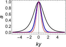
(a) The warp factor

(b) The scalar field

Figure 1: Shapes of the warp factor $a(y)$ and the scalar field $\phi(y)$ in model 1. The parameters are set as $n=1$ for the black lines, $n=3$ for the thick blue lines, and $n=5$ for the dashed red lines.

$$U(\phi)= ~{}k^{2}n^{2}v^{2}\tilde{\phi}^{\frac{2(n-1)}{n}}\left(\tilde{\phi}^{\frac{2}{n}}-1\right)^{2},$$ (17)

$$V(\phi)= ~{}k^{2}n\biggl{(}8\alpha k^{2}(n+1)(n+6)(5n+2)\tilde{\phi}^{4}$$

$$~{}-\left(8\alpha k^{2}(n(37n+56)+16)+6n+3\right)\tilde{\phi}^{2}$$

$$~{}+32k^{2}(\alpha+3\alpha n)+3\biggr{)},$$ (18)

$$\lambda(\phi)= ~{}\frac{\tilde{\phi}^{2-2n}}{2nv^{2}\left(1-\tilde{\phi}^{2}\right)^{2}}\biggl{(}8\alpha k^{2}(5n+2)(n(3n+2)-6)\tilde{\phi}^{4}$$

$$~{}+\left(3-32\alpha k^{2}(n(4n-9)-4)\right)\tilde{\phi}^{2}$$

$$~{}-\left(16\alpha k^{2}(5n+2)+3\right)\biggr{)},$$ (19)

where $\tilde{\phi}=\frac{\phi}{v}$.

Considering the condition (14) in this model, we obtain the range of $k^{2}\alpha$:

$$-\frac{1}{16n}<k^{2}\alpha<\frac{1}{40n^{2}}.$$ (20)

Here we show the shapes of the dimensionless energy density $\rho/k^{2}$ in Fig. 2 for several situations. Besides, it is found that the brane will spilt into two sub-branes when $-\frac{1}{16n}<k^{2}\alpha<-\frac{1}{8n(4+5n)}$.

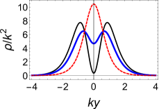
(a) $n=1$

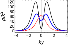
(b) $n=3$

Figure 2: The energy density of model 1 with $v=1$, and $n=1$ (the left panel) and $n=3$ (the right panel). In the left panel we set $k^{2}\alpha=-0.06$ for the black line, $k^{2}\alpha=-0.03$ for the thick blue line, and $k^{2}\alpha=0.01$ for the dashed red line. In the right panel we set $k^{2}\alpha=-0.018$ for the black line, $k^{2}\alpha=-0.0073$ for the thick blue line, and $k^{2}\alpha=0.00014$ for the dashed red line.

II.2 Model 2

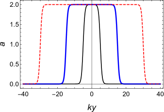
Figure 3: The warp factor of model 2. The parameter $v$ is set to $v=1$, and $kb=5$ for the black line, $kb=15$ for the thick blue line, and $kb=30$ for the dashed red line.

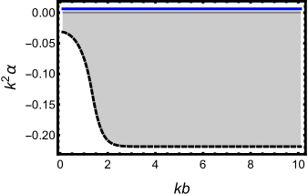
Figure 4: Plot of the range (the dark region) of $k^{2}\alpha$ and $kb$ in the condition of $f_{R}>0$ for model 2.

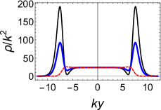
(a) $kb=7$

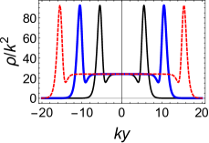
(b) $k^{2}\alpha=-0.008$

Figure 5: The energy density of model 2. The parameter $v$ is set to $v=1$. In the left panel, we set $kb=7$, and $k^{2}\alpha=-0.018$ for the black line, $k^{2}\alpha=-0.008$ for the thick blue line, and $k^{2}\alpha=0.006$ for the dashed red line. In the right panel, we set $k^{2}\alpha=-0.008$, and $kb=5$ for the black line, $kb=10$ for the thick blue line, and $kb=15$ for the dashed red line.

In the second model, the warp factor has a platform near the origin of the extra dimension, which can be seen from Fig. 3. The scalar field is a single-kink configuration. The expressions of the warp factor, the scalar field, and the scalar potential $U$ are given by

$$a(y) =\text{tanh}[k(y+b)]-\text{tanh}[k(y-b)],$$ (21)

$$\phi(y) =v\,\text{tanh}(ky),$$ (22)

$$U(\phi) =\frac{k^{2}}{v^{2}}\left(\phi^{2}-v^{2}\right)^{2}.$$ (23)

Here we do not show the complicated $V(\phi)$ and $\lambda(\phi)$, which can be solved analytically. Note that the width of the platform of the warp factor is controlled by the parameter $kb$. Considering the condition (14), we can obtain the range of the parameter $k^{2}\alpha$ numerically, which is shown in Fig. 4. From this figure, we can see that when $kb\gtrsim 2$ the range of $k^{2}\alpha$ is of about

$$-0.219<k^{2}\alpha<0.00625.$$ (24)

The dimensionless energy density $\rho/k^{2}$ in this model is shown in Fig. 5. The brane will split into multi-branes for $kb\gtrsim 2$ with $k^{2}\alpha$ in the range of (24). When $kb$ close to zero the warp factor and the energy density will close to model 1 with $n=1$. In other words, whether the brane split or not depends on the value of $k^{2}\alpha$, when $k^{2}\alpha$ is smaller than some value the brane will split into two sub-branes.

We can also extend this warp factor to the form as follows

$$a(y)= ~{}\text{tanh}[k(y-b-d)]-\text{tanh}[k(y+b+d)]$$

$$-\text{tanh}[k(y+d)]+\text{tanh}[k(y-d)],$$ (25)

where $b$ and $d$ are positive parameters. Using this warp factor one can construct a brane world with double number of sub-branes, which will be further investigated in Sec. IV.

II.3 Model 3

The third model is

$$a(y)= ~{}\text{sech}(k(y-b))+\text{sech}(ky)$$

$$~{}+\text{sech}(k(y+b)),$$ (26)

$$\phi(y)= ~{}v\,\text{tanh}(ky),$$ (27)

$$U(\phi)= ~{}\frac{k^{2}}{v^{2}}(\phi^{2}-v^{2})^{2}.$$ (28)

The scalar field is also a single-kink and the warp factor has peaks for large parameter $kb$, which can be seen from Fig. 6(a). Here we also do not show the complicated expressions of $\lambda(\phi)$ and $V(\phi)$.

The range of $k^{2}\alpha$ due to the condition $f_{R}>0$ is shown in Fig. 7. We can see that for $kb\gtrsim 4$, the range of $k^{2}\alpha$ is $-0.0625<k^{2}\alpha<0.025$. The dimensionless energy density $\rho/k^{2}$ for $kb=5$ in this model is shown in Fig. 6(b). In this situation, the sub-branes will always exist for $kb\gtrsim 4$ and $k^{2}\alpha$ in the range we obtained. When $kb$ close to zero, the warp factor and the energy density will also close to model 1 with $n=1$. In other words, whether the brane split or not for the case of small $kb$ depends on the value of $k^{2}\alpha$. When $k^{2}\alpha$ less than some critical value the brane will split into two sub-branes.

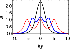
(a) The warp factor

(b) The energy density

Figure 6: The warp factor and the energy density of model 3. The parameter $v$ is set to $v=1$. In the left panel we set $kb=1$ for the black line, $kb=3$ for the thick blue line, and $kb=5$ for the dashed red line. In the right panel we set $kb=5$ and $k^{2}\alpha=-0.06$ for the black line, $k^{2}\alpha=-0.03$ for the thick blue line, and $k^{2}\alpha=0.02$ for the dashed red line.

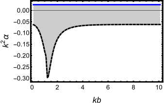
Figure 7: Plot of the range (the dark region) of $k^{2}\alpha$ and $kb$ in the condition of $f_{R}>0$ for model 3.

We can also extend this three-peak model to multiple-peak model with the following warp factor

$$a(y)=\sum^{N}_{n=-N}\text{sech}(k(y+nb)),$$ (29)

where $N$ is an arbitrary positive integer.

III Tensor perturbations and localization

In this section, we investigate the stability of the system by studying the tensor perturbation. The perturbed metric is given by

$$g_{MN}=\bar{g}_{MN}+\delta g_{MN},$$ (30)

with

$$\bar{g}_{MN}=\begin{pmatrix}a^{2}(y)\eta_{\mu\nu}&0\\ 0&1\end{pmatrix},\quad\delta g_{MN}=\begin{pmatrix}a^{2}(y)h_{\mu\nu}&0\\ 0&0\end{pmatrix},$$ (31)

where $h_{\mu\nu}=h_{\mu\nu}(x^{\rho},y)$ depends on all coordinates. Here, we only consider the tensor perturbation, so $\delta g_{5N}=0$. Using the relation $g^{NP}g_{PM}=\delta^{N}_{M}$, one can obtain the inverse of $\delta g_{MN}$,

$$\delta g^{MN}=\begin{pmatrix}-a^{-2}(y)h^{\mu\nu}&0\\ 0&0\end{pmatrix},$$ (32)

where $h^{\mu\nu}=\eta^{\mu\lambda}\eta^{\nu\rho}h_{\lambda\rho}$. Note that, we only keep the first order. Then the following relations can be obtained

$$\delta R_{\mu\nu}= -\frac{1}{2}\left(\square^{(4)}h_{\mu\nu}+\partial_{\mu}\partial_{\nu}h-\partial_{\nu}\partial_{\sigma}h^{\sigma}_{\mu}-\partial_{\mu}\partial_{\sigma}h^{\sigma}_{v}\right)$$

$$-2aa^{\prime}h^{\prime}_{\mu\nu}-3h_{\mu\nu}a^{\prime 2}-ah_{\mu\nu}a^{\prime\prime}-\frac{1}{2}a^{2}h^{\prime\prime}_{\mu\nu}$$

$$-\frac{1}{2}a\eta_{\mu\nu}a^{\prime}h^{\prime},$$ (33)

$$\delta R_{\mu 5}= \frac{1}{2}\partial_{y}\left(\partial_{\lambda}h^{\lambda}_{\mu}-\partial_{\mu}h\right),$$ (34)

$$\delta R_{55}= -\frac{1}{2}\left(\frac{2a^{\prime}h^{\prime}}{a}+h^{\prime\prime}\right),$$ (35)

$$\delta R= -\frac{\square^{(4)}h}{a^{2}}+\frac{\partial_{\mu}\partial_{\nu}h^{\mu\nu}}{a^{2}}-\frac{a^{\prime}}{a}5h^{\prime}-h^{\prime\prime}.$$ (36)

Here $\square^{(4)}=\eta^{\mu\nu}\partial_{\mu}\partial_{\nu}$ is the four-dimensional d’Alembert operator, and $h=\eta^{\mu\nu}h_{\mu\nu}$ is the trace of the tensor perturbation. Hereafter, we use the transverse-traceless gauge $h=0=\partial_{\mu}h^{\mu}_{\nu}$. Then, Eqs. (33)-(36) can be simplified further. Using the above relations, we obtain the tensor perturbation equation

$$-\frac{1}{4}a^{2}h_{\mu\nu}f(R)+\frac{1}{2}a^{2}h_{\mu\nu}V-\frac{1}{2}\lambda a^{2}h_{\mu\nu}\left[\phi^{\prime 2}-U(\phi)\right]$$

$$\quad+\frac{1}{2}\left(-\frac{1}{2}\square^{(4)}h_{\mu\nu}-3a^{\prime 2}h_{\mu\nu}-2aa^{\prime}h^{\prime}_{\mu\nu}-aa^{\prime\prime}h_{\mu\nu}\right.$$

$$\left.-\frac{a^{2}}{2}h^{\prime\prime}_{\mu\nu}\right)f_{R}+a^{2}\left[\frac{1}{2}h_{\mu\nu}\left(3\frac{a^{\prime}}{a}f^{\prime}_{R}+f^{\prime\prime}_{R}\right)-\frac{1}{4}h^{\prime}_{\mu\nu}f^{\prime}_{R}\right]=0.$$ (37)

Comparing with the Einstein equation (3), one can easily obtain

$$\left(a^{-2}\square^{(4)}h_{\mu\nu}+4\frac{a^{\prime}}{a}h^{\prime}_{\mu\nu}+h^{\prime\prime}_{\mu\nu}\right)f_{R}+h^{\prime}_{\mu\nu}f^{\prime}_{R}=0.$$ (38)

After the coordinate transformation $dz=a^{-1}dy$, we can rewrite the perturbed equation (38) as

$$\left[\partial^{2}_{z}+\left(3\frac{\partial_{z}a}{a}+\frac{\partial_{z}f_{R}}{f_{R}}\right)\partial_{z}+\square^{(4)}\right]h_{\mu\nu}=0.$$ (39)

Considering the Kaluza-Klein (KK) decomposition $h_{\mu\nu}(x^{\rho},z)=\left(a^{-3/2}f_{R}^{-1/2}\right)\epsilon_{\mu\nu}(x^{\rho})\psi(z)$, where $\epsilon_{\mu\nu}(x^{\rho})$ satisfies the transverse and traceless conditions $\eta^{\mu\nu}\epsilon_{\mu\nu}=0$ and $\partial_{\mu}\epsilon^{\mu}_{\nu}=0$, we obtain the following Schrödinger-like equation for the extra-dimensional part $\psi(z)$

$$\left[-\partial^{2}_{z}+W(z)\right]\psi(z)=m^{2}\psi(z),$$ (40)

where

$$W(z)= ~{}\frac{3}{4}\frac{(\partial_{z}a)^{2}}{a^{2}}+\frac{3}{2}\frac{\partial_{z}a~{}\partial_{z}f_{R}}{af_{R}}$$

$$-\frac{1}{4}\frac{(\partial_{z}f_{R})^{2}}{f^{2}_{R}}+\frac{3}{2}\frac{\partial_{z}^{2}a}{a}+\frac{1}{2}\frac{\partial_{z}^{2}f_{R}}{f_{R}},$$ (41)

is the effective potential of gravitons. The effective potential (41) in $y$ coordinate is

$$W(z(y))=\frac{9}{4}a^{\prime 2}+2\frac{aa^{\prime}f^{\prime}_{R}}{f_{R}}-\frac{1}{4}a^{2}\frac{f^{\prime 2}_{R}}{f^{2}_{R}}+\frac{3}{2}aa^{\prime\prime}+\frac{1}{2}\frac{a^{2}f^{\prime\prime}_{R}}{f_{R}}.$$ (42)

It would be clearer if Eq. (40) is written in the following form

$$QQ^{\dagger}\psi(z)=m^{2}\psi(z),$$ (43)

with

$$Q=\partial_{z}+\left(\frac{3}{2}\frac{\partial_{z}a}{a}+\frac{1}{2}\frac{\partial_{z}f_{R}}{f_{R}}\right),$$ (44)

$$Q^{\dagger}=-\partial_{z}+\left(\frac{3}{2}\frac{\partial_{z}a}{a}+\frac{1}{2}\frac{\partial_{z}f_{R}}{f_{R}}\right).$$ (45)

Equation (43) guarantees that there is no tachyonic KK graviton with $m^{2}<0$. So, the system is stable under the tenser perturbation.

The solution of the graviton zero mode is

$$\psi^{(0)}(z)=\sqrt{N_{0}a^{3}(z)f_{R}(z)},$$ (46)

where $N_{0}$ is the normalization constant. The zero mode $\psi^{(0)}(z)$ is in fact the massless graviton. It should be normalizable in order to recover the four-dimensional Newtonian gravity. Thus, we should have the following normalization condition

$$\mathcal{I}\equiv\int^{\infty}_{-\infty}\left|\psi^{(0)}(z)\right|^{2}dz=1.$$ (47)

Considering the solution (46) and the coordinate transformation $dz=a^{-1}dy$, the above condition reads as

$$\mathcal{I}= \int^{\infty}_{-\infty}N_{0}a^{2}(y)f_{R}(y)dy$$

$$= \int^{\infty}_{-\infty}N_{0}\left[a^{2}(y)-24\alpha a^{\prime}(y)^{2}-16\alpha a(y)a^{\prime\prime}(y)\right]dy=1.$$ (48)

For model 1, the graviton zero mode can be normalized and the normalization constant is given by

$$N_{0}=\frac{n(n+1)}{(8n^{2}k^{2}\alpha-2n-1){}_{2}F_{1}(1,-1-n;1+n;-1)},$$ (49)

where ${}_{2}F_{1}$ is the hypergeometric function. It can be seen that this value is positive and finite when $n$ is a positive integer.

For models 2 and 3, we have respectively

$$N_{0}^{-1}= ~{}8kb\coth(2kb)-4-\frac{16}{3}k^{2}\alpha\text{csch}^{3}(2kb)\Big{[}9\sinh(2kb)$$

$$+\sinh(6kb)-24kb\cosh(2kb)\Big{]},$$ (50)

$$N_{0}^{-1}= ~{}6+4kb\text{csch}(kb)(2+\text{sech}(kb))-4k^{2}\alpha\text{csch}^{3}(2kb)\times$$

$$\Big{[}-24kb-8kb\Big{(}22\cosh(kb)+9\cosh(3kb)$$

$$+\cosh(4kb)+\cosh(5kb)\Big{)}+\sinh(6kb)$$

$$+16\sinh(5kb)+8\sinh(4kb)+48\sinh(3kb)$$

$$-3\sinh(2kb)+32\sinh(kb)\Big{]}.$$ (51)

This means that the graviton zero mode for each model considered in this paper can be localized near the brane Csaki2000 ; Soda2002 . The effective potentials and the graviton zero modes for the three models are shown in Fig. 8. From the analysis above of this section we notice that the tenser perturbation in mimetic $f(R)$ gravity is the same as that in $f(R)$ gravity ZhongYuan2011 . The reason is that the tenser perturbation is independent of the mimetic scalar field. And this result is also consistent with the mimetic brane world ZhongYi2018 . But the mimetic scalar field gives a degree of freedom which could generate more abundant inner structure.

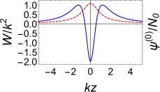
(a) Model 1

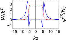
(b) Model 2

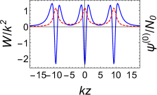
(c) Model 3

Figure 8: The effective potentials (the blue lines) and the corresponding graviton zero modes (the red dashed lines) for the three models. For model 1, we set $v=1$ and $k^{2}\alpha=0.01$; for model 2, $v=1$, $kb=10$, and $k^{2}\alpha=0.006$; and for model 3, $v=1$, $kb=5$, and $k^{2}\alpha=0.02$.

IV The gravitational resonances of mimetic $f(R)$ brane

The abundant inner structure of the effective potential may lead to some interesting KK resonant behavior which will be studied in this section.

To get numerical solutions of Eq. (40), a convenient way is to impose the following boundary conditions for the KK modes

$$\psi_{\text{even}}(0)=1, \quad\partial_{z}\psi_{\text{even}}(0)=0;$$ (52)

$$\psi_{\text{odd}}(0)=0, \quad\partial_{z}\psi_{\text{odd}}(0)=1,$$ (53)

where $\psi_{\text{even}}$ and $\psi_{\text{odd}}$ denote even and odd parity KK modes of $\psi(z)$, respectively. The integration of the function $\left|\psi(z)\right|^{2}$ can be considered as the probability of finding massive KK gravitons along the extra dimension. In order to find gravitational KK resonances, one can define the relative probability Liu2009 :

$$P(m^{2})=\frac{\int^{z_{b}}_{-z_{b}}|\psi(z)|^{2}dz}{\int^{z_{\text{max}}}_{-z_{\text{max}}}|\psi(z)|^{2}dz},$$ (54)

where $2z_{b}$ is the approximate width of the brane and $z_{\text{max}}$ can be taken as $10z_{b}$. For a given $m^{2}$, using conditions (52) and (53), the even parity KK mode $\psi_{\text{even}}$ and the odd parity KK mode $\psi_{\text{odd}}$ can be solved numerically from the Schrödinger-like equation (40). In this case, the relative probability $P$ corresponding to $\psi_{\text{even}}$ or $\psi_{\text{odd}}$ can be obtained. As a function of $m^{2}$, the relative probability will have a peak for some value of $m^{2}$. Then we may regard this mode as a gravitational KK resonance. Actually, we treat it as a KK resonance only when the corresponding peak has a full width at half maximum $\Gamma$, i.e., the width of the half height of the peak value. We can define the lifetime of the gravitational KK resonance as $\tau=\Gamma^{-1}$.

Next, we will investigate gravitational KK resonances in three cases. Before that, in order to investigate conveniently we introduce some dimensionless parameters. Using the parameter $k$, we can define the following dimensionless parameters $\bar{y}=ky$, $\bar{z}=kz$, $\bar{b}=kb$, $\bar{\tau}=k\tau$, $\bar{\Gamma}=\Gamma/k$, $\bar{m}=m/k$, $\bar{W}=W/k^{2}$, and $\bar{\alpha}=k^{2}\alpha$. In our system, both parameters $\bar{b}$ and $\bar{\alpha}$ can affect the KK resonance behavior. The effects of the parameter $\bar{b}$ has been investigated in Refs. ZhongYi2019 ; Fu2014 ; Tan2020 , so in this paper, we will focus on the effects of the parameter $\bar{\alpha}$, which can measure the deviation from mimetic gravity.

IV.1 Case 1

We begin with the following warp factor

$$a(\bar{y})=\tanh(\bar{y}+\bar{b})-\tanh(\bar{y}-\bar{b}).$$ (55)

In this case we choose $\bar{b}=10$ as a specific example to investigate gravitational KK resonances. So from Eq. (24) we know that $\bar{\alpha}$ has two bounds. Effects of the parameter $\bar{\alpha}$ on the effective potential can be seen from Fig. 9. From this figure we can see that, the height of the two big barriers decreases rapidly with $\bar{\alpha}$. When $\bar{\alpha}$ approaches to zero, the barriers will disappear. Besides, the depth of the effective potential will decrease first and then increase with $\bar{\alpha}$. It is worth to note that in Ref. Xu2015 the KK resonances were found when $\bar{\alpha}$ is out of the range of Eq. (14).

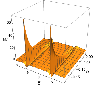
Figure 9: The effect of the parameter $\bar{\alpha}$ on the effective potential with $\bar{b}=10$ for case 1.

In this case we set $\bar{z}_{b}$ in the relative probability (54) as $\bar{z}_{b}=6.5$. For $\bar{\alpha}=-0.19$, $-0.14$, and $-0.0012$ we can obtain the relative probabilities. Then, the corresponding effective potentials, the relative probabilities, and the wave functions of the first odd and even KK resonances are shown in Figs. 10, 11, and 12. From Figs. 10(a), 11(a), and 12(a), we can see that, the height of the effective potential barrier decreases with the parameter $\bar{\alpha}$. Besides, from Figs. 10(b) and 11(b) we can see that the peak values do not decrease with $\bar{m}^{2}$ monotonously, which is an unusual phenomenon.

(a) The effective potential

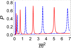
(b) The relative probability

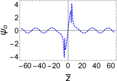
(c) The first odd wave function with $\bar{m}^{2}=0.0831$

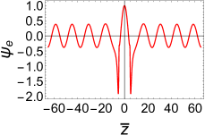
(d) The first even wave function with $\bar{m}^{2}=0.2045$

Figure 10: The effective potential, the relative probability, and the wave functions of the first odd and even KK resonances with $\bar{b}=10$ and $\bar{\alpha}=-0.19$ for case 1.

(a) The effective potential

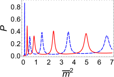
(b) The relative probability

(c) The first odd wave function with $\bar{m}^{2}=0.0924$

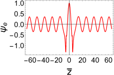
(d) The first even wave function $\bar{m}^{2}=0.2945$

Figure 11: The effective potential, the relative probability, and the wave functions of the first odd and even KK resonances with $\bar{b}=10$ and $\bar{\alpha}=-0.14$ for case 1.

(a) The effective potential

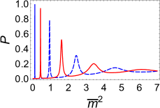
(b) The relative probability

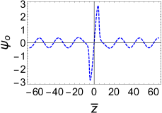
(c) The first odd wave function with $\bar{m}^{2}=0.1087$

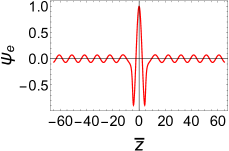
(d) The first even wave function with $\bar{m}^{2}=0.4277$

Figure 12: The effective potential, the relative probability, and the wave functions of the first odd and even KK resonances with $\bar{b}=10$ and $\bar{\alpha}=-0.0012$ for case 1.

We are also interested in the first gravitational KK resonance, its lifetime $\bar{\tau}_{1}$ and the mass square $\bar{m}^{2}$ for different values of $\bar{\alpha}$ are shown in Fig. 13. They can be fitted as the following two functions

$$\bar{m}^{2} =0.102\bar{\alpha}+0.109,$$ (56)

$$\bar{\tau}_{1} =\frac{1}{0.00335-0.447\bar{\alpha}}+132.$$ (57)

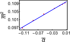
(a) $\bar{m}^{2}$

(b) $\bar{\tau}_{1}$

Figure 13: The effects of the parameter $\bar{\alpha}$ on the mass square $\bar{m}^{2}$ and the lifetime $\bar{\tau}$ of the first KK resonance for case 1. Red dots are numerical results, blue solid lines are fit functions. In the left panel the fit function is $\bar{m}^{2}=0.102\bar{\alpha}+0.109$, in the right panel the fit function is $\bar{\tau}_{1}=\frac{1}{0.00335-0.447\bar{\alpha}}+131.621$.

From Eq. (56) we can see that the mass square $\bar{m}^{2}$ of the first KK resonance linearly increases with the parameter $\bar{\alpha}$. And from Eq. (57) we can see that the lifetime of the first KK resonance increases with $\bar{\alpha}$ slowly first and then rapidly when $\bar{\alpha}$ closes to the upper bound.

IV.2 Case 2

In this case, we investigate the brane world with three sub-branes, for which the warp factor is

$$a(\bar{y})=\text{sech}(\bar{y}-\bar{b})+\text{sech}(\bar{y})+\text{sech}(\bar{y}+\bar{b}).$$ (58)

Without loss of generality we choose $\bar{b}=5$ as a specific example, and the corresponding range of $\bar{\alpha}$ is $-0.0642<\bar{\alpha}<0.025$. Gravitational KK resonances also exist in this kind of warp factor, but the situation will be different from case 1. The effective potential for different values of $\bar{\alpha}$ can be seen in Fig. 14. From this figure we can see that there are three sub-wells, and the effect of $\bar{\alpha}$ to the effective potential is similar to that in case 1. We fix $\bar{z}_{b}=12$ and set $\bar{\alpha}$ as -0.0581, -0.0373, and 0.0161 as examples to study the gravitational KK resonances.

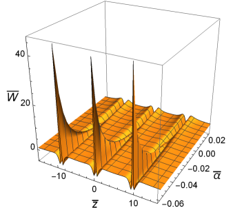
Figure 14: The effect of the parameter $\bar{\alpha}$ on the effective potential with $\bar{b}=5$ for case 2.

(a) The effective potential

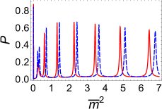
(b) The relative probability

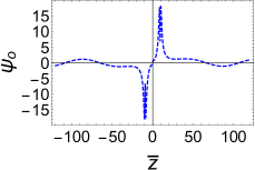
(c) The first odd wave function with $\bar{m}^{2}=0.0064$

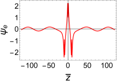
(d) The first even wave function with $\bar{m}^{2}=0.0137$

Figure 15: The effective potential, the relative probability, and wave functions of the first odd and even KK resonance with $\bar{b}=5$ and $\bar{\alpha}=-0.0581$ for case 2.

(a) The effective potential

(b) The relative probability

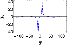
(c) The first odd wave function with $\bar{m}^{2}=0.0059$

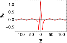
(d) The first even wave function with $\bar{m}^{2}=0.0172$

Figure 16: The effective potential, the relative probability, and wave functions of the first odd and even KK resonance with $\bar{b}=5$ and $\bar{\alpha}=-0.0373$ for case 2.

(a) The effective potential

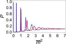
(b) The relative probability

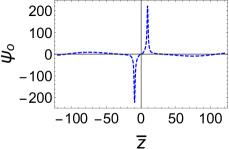
(c) The first odd wave function with $\bar{m}^{2}=0.0028$

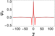
(d) The first even wave function with $\bar{m}^{2}=0.00892$

Figure 17: The effective potential, the relative probability, and wave functions of the first odd and even KK resonance with $\bar{b}=5$ and $\bar{\alpha}=0.016$ for case 2.

The shapes of the effective potential, the relative probability and the wave functions of the first odd and even KK resonances are shown in Figs. 15, 16, and 17. We can see that for some values of $\bar{\alpha}$, the relative probabilities of the KK resonances do not decrease with their masses $\bar{m}^{2}$ monotonously, which is similar to case 1. Besides, Figs. 15 and 17 show that the masses of some KK resonances are very close, which is similar to the result in Xie2020 , where the doubly degenerate phenomenon happens. Comparing the effective potential with that in Ref. Xie2020 , we can see that they both have sub-structure, and this sub-structure is the main reason of this phenomenon.

We also investigate the lifetime $\bar{\tau}_{1}$ and the mass square $\bar{m}^{2}$ of the first resonance for different values of $\bar{\alpha}$. The results are shown in Fig. 18 and we also get the following fit functions

$$\bar{m}^{2} =0.00373-0.0557\bar{\alpha},$$ (59)

$$\bar{\tau}_{1} =\frac{10000}{14.3-540\bar{\alpha}}+238.$$ (60)

From Eq. (59), one can see that the mass square $\bar{m}^{2}$ of the first KK resonance linearly decreases with the parameter $\bar{\alpha}$, which is different from case 1. Equation (60) shows that the lifetime increases with $\bar{\alpha}$ slowly first and then rapidly, just like the case 1.

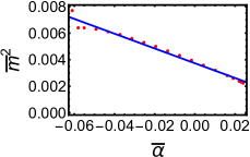
(a) $\bar{m}^{2}$

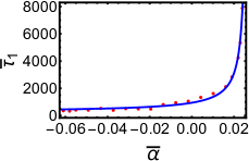
(b) $\bar{\alpha}$

Figure 18: The effects of $\bar{\alpha}$ to the scaled mass $\bar{m}^{2}$ and the scaled lifetime $\bar{\tau}_{1}$ of the first KK resonance for case 2. Red dots are numerical results and solid blue lines are fit functions. In the left panel the fit function is $\bar{m}^{2}=0.00373-0.0557\bar{\alpha}$, in the right panel the fit function is $\bar{\tau}_{1}=\frac{1}{14.3-540\bar{\alpha}}+0.0238$.

From case 1 and case 2, we find that, when $\bar{\alpha}$ is small, there is an unusual phenomenon, i.e., the peak values of the relative probability of the KK resonances do not decrease monotonously with $\bar{m}^{2}$. This phenomenon appears when $\bar{\alpha}\lesssim-0.024$ for case 1 and $\bar{\alpha}\lesssim-0.014$ for case 2.

IV.3 Case 3

In this case, we will focus on the gravitational KK resonances quasi-localized in sub-wells and between sub-wells. The warp factor is

$$a(\bar{y})= \text{tanh}(\bar{y}-\bar{b}-\bar{d})-\text{tanh}(\bar{y}+\bar{b}+\bar{d})$$

$$-\text{tanh}(\bar{y}+\bar{d})+\text{tanh}(\bar{y}-\bar{d}).$$ (61)

Compared with case 1, this warp factor has two platforms and the effective potential has more abundant sub-structure, which can be seen in Fig. 19.

From case 1 we have found that for large $\bar{b}$ the range of $\bar{\alpha}$ is $-0.219<\bar{\alpha}<0.00625$. In the current case we set $\bar{b}=13$ and $\bar{d}=2.3$, for which the range of $\bar{\alpha}$ is still $-0.219<\bar{\alpha}<0.00625$.

The effective potential for different values of $\bar{\alpha}$ is shown in Fig. 20. In order to investigate the KK resonances only quasi-localized in sub-wells, we need to redefine the corresponding relative probability $P_{s}$ ZhongYi2019 :

$$P_{s}=\left\{\begin{array}[]{cl}\frac{\int_{\bar{z}_{1}}^{\bar{z}_{2}}|\psi(\bar{z})|^{2}d\bar{z}}{\int_{\bar{z}_{m}-5\left(\bar{z}_{2}-\bar{z}_{1}\right)}^{\bar{z}_{m}+5\left(\bar{z}_{2}-\bar{z}_{1}\right)}|\psi(\bar{z})|^{2}d\bar{z}},&\bar{z}_{m}\geq 5\left(\bar{z}_{2}-\bar{z}_{1}\right)\\ &\\ \frac{\int_{\bar{z}_{1}}^{\bar{z}_{2}}|\psi(\bar{z})|^{2}d\bar{z}}{\int_{0}^{10\left(\bar{z}_{2}-\bar{z}_{1}\right)}|\psi(\bar{z})|^{2}d\bar{z}},&\bar{z}_{m}<5\left(\bar{z}_{2}-\bar{z}_{1}\right)\end{array}\right.$$ (62)

where $\bar{z}_{1}$ and $\bar{z}_{2}$ are the left and right edges of the right sub-well respectively (as Fig. 19(b) shows), and $\bar{z}_{m}=\frac{\bar{z}_{1}+\bar{z}_{2}}{2}$. Besides, between two sub-wells there is also a potential well, and KK resonances can also be quasi-localized in it. We also need to redefine the relative probability in this region ZhongYi2019 :

$$P_{m}=\frac{\int^{\bar{z}_{1}}_{-\bar{z}_{1}}|\psi(\bar{z})|^{2}d\bar{z}}{\int^{10\bar{z}_{1}}_{-10\bar{z}_{1}}|\psi(\bar{z})|^{2}d\bar{z}}.$$ (63)

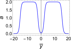
(a) The warp factor

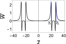
(b) The effective potential

Figure 19: The warp factor and the effective potential $W(\bar{z})$ for case 3. The parameters are set as $\bar{b}=13$, $\bar{d}=2.3$, and $\bar{\alpha}=-0.00126$.

Figure 20: The effect of the parameter $\bar{\alpha}$ on the effective potential with $\bar{b}=13$ and $\bar{d}=2.3$ for case 3.

We solve the Shrödinger-like equation (40) numerically with the boundary conditions (52) and (53). Using the redefined relative probabilities (62) and (63), one can get the gravitational KK resonances. Figures 21, 23, and 25 show the effective potential and the corresponding relative probability for $\bar{\alpha}=-0.189$, $\bar{\alpha}=-0.0838$, and $\bar{\alpha}=-0.00126$, respectively. Through these figures we can see that the effects of $\bar{\alpha}$ on the effective potentials and relative probability are very considerable. Compared with the results of mimetic gravity brane world (see Fig. 11(c) in Ref. ZhongYi2019 ), we find that relative probabilities of KK resonances in sub-wells for small $\bar{\alpha}$ are much larger, which can be seen in Fig. 21(c). As $\bar{\alpha}$ approaches to zero, mimetic $f(R)$ gravity goes go back to mimetic gravity and the results of gravitational KK resonances also recover to that of in mimetic gravity ZhongYi2019 .

From Figs. 21(c), 23(c), and 25(c) we can see that the peaks of relative probabilities of gravitational KK resonances in the sub-wells appear in clusters. And the main peak value of each cluster does not monotonically decrease with $\bar{m}^{2}$ when $\bar{\alpha}$ is small, this is because the sub-wells also have their sub-structure changing with $\bar{\alpha}$. From Figs. 21(b), 23(b), and 25(b) we can also see that the peak values of relative probabilities of gravitational KK resonances quasi-localized between sub-wells will not monotonically decrease with $\bar{m}^{2}$. Besides, comparing the above two cases, we see that there are no corresponding KK resonances with large relative probabilities $P_{m}$ at the locations of the main peaks of clusters in $P_{s}$. This is caused by the existence of sub-structure of the effective potential. The wave functions of KK resonances quasi-localized both between sub-wells and in sub-wells are shown in Figs. 22, 24, and 26 for corresponding $\bar{\alpha}$.

On the other hand, from Figs. 21(c), 23(c), and 25(c) we find that the mass square $\bar{m}^{2}$ of the first odd parity KK resonance and the first even parity KK resonance are very close. One could also regard this as doubly degenerate Xie2020 .

(a) The effective potential

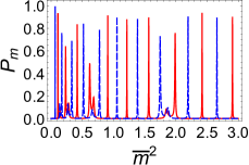
(b) The relative probability $P_{m}$

(c) The relative probability $P_{s}$

Figure 21: The effective potential, the relative probabilities of the even parity KK mode $\psi_{e}$ (dashed blue lines) and the odd parity KK mode $\psi_{o}$ (solid red lines) quasi-localized between the sub-wells $P_{m}$ and in the sub-wells $P_{s}$ with $\bar{b}=13$, $\bar{d}=2.3$, and $\bar{\alpha}=-0.189$ for case 3.

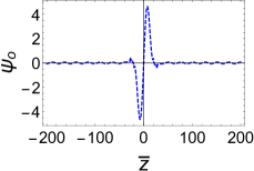
(a) The first odd wave function quasi-localized between sub-wells with $\bar{m}^{2}=0.0652$

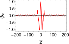
(b) The first even wave function quasi-localized between sub-wells with $\bar{m}^{2}=0.110$

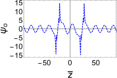
(c) The first odd wave function quasi-localized in sub-well with $\bar{m}^{2}=0.137$

(d) The first even wave function quasi-localized in sub-well with $\bar{m}^{2}=0.142$

Figure 22: Resonances quasi-localized between sub-wells and in sub-wells with $\bar{b}=13$, $\bar{d}=2.3$, and $\bar{\alpha}=-0.189$ for case 3.

(a) The effective potential

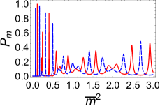
(b) The relative probability $P_{m}$

(c) The relative probability $P_{s}$

Figure 23: The effective potential, the relative probabilities of the even parity KK mode $\psi_{e}$ (dashed blue lines) and the odd parity KK mode $\psi_{o}$ (solid red lines) quasi-localized between the sub-wells $P_{m}$ and in the sub-wells $P_{s}$ with $\bar{b}=13$, $\bar{d}=2.3$, and $\bar{\alpha}=-0.0838$ for case 3.

(a) The first odd wave function quasi-localized between sub-wells with $\bar{m}^{2}=0.065$

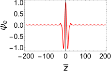
(b) The first even wave function quasi-localized between sub-wells with $\bar{m}^{2}=0.1112$

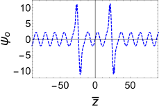
(c) The fist odd wave function quasi-localized in sub-well with $\bar{m}^{2}=0.225$

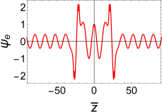
(d) The first even wave function quasi-localized in sub-well with $\bar{m}^{2}=0.217$

Figure 24: The KK resonances between sub-wells and in a sub-well with $\bar{b}=13$, $\bar{d}=2.3$, and $\bar{\alpha}=-0.0838$ for case 3.

(a) The effective potential

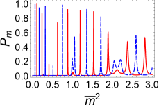
(b) The relative probability $P_{m}$

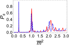
(c) The relative probability $P_{s}$

Figure 25: The effective potential, the relative probabilities of the even parity KK mode $\psi_{e}$ (dashed blue lines) and the odd parity KK mode $\psi_{o}$ (solid red lines) quasi-localized between the sub-wells $P_{m}$ and in the sub-wells $P_{s}$ with $\bar{b}=13$, $\bar{d}=2.3$, and $\bar{\alpha}=-0.00126$ for case 3.

(a) The first odd wave function quasi-localized between sub-wells with $\bar{m}^{2}=0.0608$

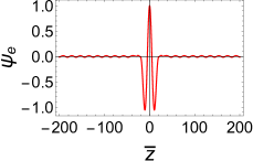
(b) The first even wave function quasi-localized between sub-wells with $\bar{m}^{2}=0.108$

(c) The fist odd wave function quasi-localized in sub-well with $\bar{m}^{2}=0.268$

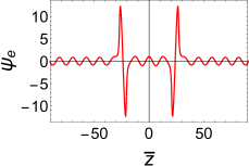
(d) The first even wave function quasi-localized in sub-well with $\bar{m}^{2}=0.268$

Figure 26: The KK resonances between sub-wells and in a sub-well with $\bar{b}=13$, $\bar{d}=2.3$, and $\bar{\alpha}=-0.00126$ for case 3.

V Conclusions and discussions

In this work, we studied the brane world system in mimetic $f(R)$ gravity. Due to the existence of the mimetic scalar field, we can get thick branes with abundant inner structure. We gave three kinds of solutions of the thick brane model for $f(R)=R+\alpha R^{2}$.

Then we investigated the stability of mimetic $f(R)$ brane world, and found that the system is stable under the tenser perturbation. The existence of the normalized graviton zero mode indicates that four-dimensional gravity can be restored. The result is same as the tensor perturbation of $f(R)$-branes in Ref. ZhongYuan2011 , this is because that the tenser perturbation is independent of the mimetic scalar field.

After that, we studied the gravitational KK resonances, which are quasi-localized on the brane. We only studied the effects of the parameter $\alpha$ on the behavior of the KK resonances. We found that for a small $\alpha$, the effective potential has a sub-structure which leads to an unusual phenomenon in the KK resonance spectrum. The lifetime of the first KK resonance increases rapidly while $\alpha$ close to its upper bound. In case 3 we focused on gravitational KK resonances quasi-localized in sub-wells and between sub-wells. We found that KK resonances can be quasi-localized both in sub-wells and between sub-wells. If $\alpha$ tends to zero the result would tend to mimetic gravity brane world in Ref. ZhongYi2019 . Compared with Ref. ZhongYi2019 , the relative probabilities of KK resonances in the sub-wells are more obvious and the main peak values of the clusters do not monotonically decrease with $\bar{m}^{2}$ for a small $\alpha$. Besides, the phenomenon of gravitational KK resonance doubly degenerate also appears when we studied KK resonances quasi-localized in a sub-well.

We note that it is proper to set the five-dimensional fundamental mass scale $M_{*}$ as unity rather than the Planck mass. In this model the relation between the four-dimensional spacetime mass scale $M_{\text{Pl}}$ and five-dimensional spacetime fundamental mass scale $M_{*}$ is as follows

$$M^{2}_{\text{Pl}}=M_{*}^{3}\int^{\infty}_{-\infty}a(z)^{3}f_{R}dz,$$ (64)

which means the four-dimensional mass scale is effective. The five-dimensional fundamental scale is determined by the warp factor and $f(R)$. And we use the parameter $k$ to recover dimensions of parameters $y$, $z$, $b$, $d$, $\tau$, $\Gamma$, $m$, $W$, and $\alpha$. For example, if we set $k=M_{*}$, for model 2, we have

$$M_{\text{Pl}}^{2}= M_{*}^{3}\Bigg{(}\frac{2}{3k}\text{csch}^{2}(2bk)\Big{(}-\left(16\alpha k^{2}+3\right)\cosh(4bk)$$

$$+6bk\big{(}16\alpha k^{2}\tanh(bk)\left(\coth^{2}(bk)+1\right)+\sinh(4bk)\big{)}$$

$$-80\alpha k^{2}+3\Big{)}\Bigg{)}.$$ (65)

If we set the parameters $kb=10$ and $k^{2}\alpha=-0.008$ then the five-dimensional spacetime fundamental mass scale can be obtain as $M_{*}=M_{\text{Pl}}/8.73=1.40\times 10^{15}~{}\text{TeV}$ from Eq. (65). And the parameter $b=1.41\times 10^{-33}~{}\text{m}$. When the energy of a particle approaches to the fundamental mass scale the effect of quantum gravity will become obvious. In this model the effect of quantum gravity is not considered. From Fig. 10 the mass of the first massive graviton is $m=\sqrt{0.0831}\times 1.40\times 10^{15}~{}\text{TeV}=1.16\times 10^{14}~{}\text{TeV}$, which is less than the fundamental mass scale. So the massive graviton can product in a collider even its energy lower than the fundamental mass scale.

At last, we discuss briefly the correction of the four-dimensional Newtonian potential from the gravitational KK modes. For the brane located around $z=z_{0}$, the four-dimensional Newtonian potential correction of a mass point $M$ is given by Csaki2000

$$U_{N}(r)\sim G_{N}\frac{M}{r}\left[1+\int_{0}^{\infty}dm~{}\mathrm{e}^{-mr}\psi_{m}^{2}\left(z_{0}\right)\right],$$ (66)

where $r$ is the distance to the mass point on the brane, and $\psi_{m}(z)$ is the normalized wave function with mass $m$ and the normalized constant $N_{m}$. In this paper if the brane is located around $z=0$, the contribution to the four-dimensional Newtonian potential is only from even KK modes. For the brane with inner structure the KK resonances that can be quasi-located at sub-brane also have contribution to the four-dimensional Newtonian potential. From Ref. Csaki2000 we know that the normalization constant $N_{m}$ is decided by the asymptotic behavior of the effective potential $W(z)$ at the boundary of the extra dimension. For the solutions considered in this paper, if we assume that $W(z)\propto\frac{\beta(\beta+1)}{z^{2}}$ and $\psi_{m}(0)\sim(m/k)^{\beta-1}$ at $z\gg 1/k$, we find $\beta=\frac{3}{2}$, which is not associated with $\alpha$. Hence, for the brane located around $z=0$ the correction to the four-dimensional Newtonian potential is

$$U_{N}(r)\sim G_{N}\frac{M}{r}\left[1+\frac{C}{(kr)^{2}}\right],$$ (67)

where $C$ is a dimensionless constant determined by the structure of brane. Here, we only consider the asymptotic behavior of the effective potential $W(z)$ at the boundary of the extra dimension. The inner structure of the effective potential around $z=0$ should have an effect on this result. This is a difficult issue and it will be studied in our future work.

In the model of mimetic brane world with abundant inner structure, it is also interesting to investigate localization of various kinds of matter fields and the corresponding KK resonance structures, which will also be studied in our future work.

VI Acknowledgments

We would like thank Yi Zhong, Zheng-Quan Cui, Hao Yu, Bao-Min Gu, and Qin Tan for helpful discussions. This work was supported in part by the National Key Research and Development Program of China (Grant No. 2020YFC2201503), the National Natural Science Foundation of China (Grants No. 11875151, No. 11522541, and No. 12047501), the 111 Project (Grant No. B20063), and the Fundamental Research Funds for the Central Universities (Grants No. lzujbky-2019-ct06). W. D. Guo was supported by the scholarship granted by the Chinese Scholarship Council (CSC).

References

- (1) N. Arkani-Hamed, S. Dimopoulos, and G. Dvali, The hierarchy problem and new dimensions at a millimeter, Phys. Lett. B 429 (1998) 263, [arXiv:hep-ph/9803315].
- (2) L. Randall and R. Sundrum, A Large Mass Hierarchy from a Small Extra Dimension, Phys. Rev. Lett. 83 (1999) 3370.
- (3) L. Randall and R. Sundrum, An alternative to compactification, Phys. Rev. Lett. 83 (1999) 4690.
- (4) V. A. Rubakov and M. E. Shaposhnikov, Do we live inside a domain wall?, Phys. Lett. B 125 (1983) 136.
- (5) O. DeWolfe, D. Z. Freedman, S. S. Gubser, and A. Karch, Modeling the fifth dimension with scalars and gravity, Phys. Rev. D 62 (2000) 046008, [arXiv:hep-th/9909134].
- (6) C. Csáki, J. Erlich, T. J. Hollowood, and Y. Shirman, Universal aspects of gravity localized on thick branes, Nucl. Phys. B 581 (2000) 309, [arXiv:hep-th/0001033].
- (7) M. Gremm, Four-dimensional gravity on a thick domain wall, Phys. Lett. B 478 (2000) 434, [arXiv:hep-th/9912060].
- (8) A. Kehagias and K. Tamvakis, Localized gravitons, gauge bosons and chiral fermions in smooth spaces generated by a bounce, Phys. Lett. B 504 (2001) 38, [arXiv:hep-th/0010112].
- (9) A. Melfo, N. Pantoja, and J. D. Tempo, Fermion localization on thick branes, Phys. Rev. D 73 (2006) 044033, [arXiv:hep-th/0601161].
- (10) C. A. Almeida, R. Casana, M. M. Ferreira, and A. R. Gomes, Fermion localization and resonances on two-field thick branes, Phys. Rev. D 79 (2009) 125022, [arXiv:0901.3543].
- (11) Z.-H. Zhao, Y.-X. Liu, and H.-T. Li, Fermion localization on asymmetric two-field thick branes, Class. Quantum Gravity 27 (2010) 185001, [arXiv:0911.2572].
- (12) A. E. R. Chumbes, A. E. O. Vasquez, and M. B. Hott, Fermion localization on a split brane, Phys. Rev. D 83 (2011) 105010, [arXiv:1012.1480].
- (13) Y. X. Liu, Y. Zhong, Z.-H. Zhao, and H.-T. Li, Domain wall brane in squared curvature gravity, J. High Energy Phys. 2011, 135 (2011), [arXiv:1104.3188v2].
- (14) Q.-Y. Xie, H. Guo, Z.-H. Zhao, Y.-Z. Du, and Y.-P. Zhang, Spectrum structure of a fermion on Bloch branes with two scalar-fermion couplings, Class. Quantum Gravity 34 (2017) 055007, [arXiv:1510.03345].
- (15) B. M. Gu, Y. P. Zhang, H. Yu, and Y. X. Liu, Full linear perturbations and localization of gravity on brane, Eur. Phys. J. C 77 (2017) 115, [arXiv:1606.07169].
- (16) Y. Zhong and Y. X. Liu, Linearization of a warped theory in the higher-order frame, Phys. Rev. D 95 (2017) 104060.
- (17) Y. Zhong, K. Yang, and Y. X. Liu, Linearization of a warped theory in the higher-order frame II: The equation of motion approach, Phys. Rev. D 97 (2017) 044032, [arXiv:1708.03737].
- (18) X.-N. Zhou, Y.-Z. Du, H. Yu, and Y.-X. Liu, Localization of gravitino field on f(R)-thick branes, Sci. China Physics, Mech. Astron. 61 (2018) 110411, [arXiv:1703.10805].
- (19) Y. X. Liu, K. Yang, H. Guo, and Y. Zhong, Domain wall brane in Eddington-inspired Born-Infeld gravity, Phys. Rev. D 85 (2012) 124053, [arXiv:1203.2349].
- (20) Z.-G. Xu, Y. Zhong, H. Yu, and Y.-X. Liu, The structure of -brane model, Eur. Phys. J. C 75 (2015) 368, [arXiv:1405.6277].
- (21) H. Yu, Y. Zhong, B.-M. Gu, and Y.-X. Liu, Gravitational resonances on -brane, Eur. Phys. J. C 76 (2016) 195.
- (22) W. T. da Cruz, D. M. Dantas, R. V. Maluf, and C. A. S. Almeida, Configurational Entropy and Newton’s Law in Double Sine-Gordon Braneworlds, Ann. Phys. 531 (2019) 1900178, [arXiv:1810.03991].
- (23) J.-J. Wan, Z.-Q. Cui, W.-B. Feng, and Y.-X. Liu, Smooth braneworld in 6-dimensional asymptotically AdS spacetime, J. High Energy Phys. 17 (2021), [arXiv:2010.05016].
- (24) J. L. Rosa, D. A. Ferreira, D. Bazeia, and F. S. N. Lobo, Thick brane structures in generalized hybrid metric-Palatini gravity, [arXiv:2010.10074].
- (25) D. Bazeia and A. R. Gomes, Bloch brane, J. High Energy Phys. 05 (2004) 012, [arXiv:hep-th/0403141].
- (26) A. De Souza Dutra, A. C. Amaro De Faria, and M. Hott, Degenerate and critical Bloch branes, Phys. Rev. D 78 (2008) 043526, [arXiv:0807.0586].
- (27) A. D. S. Dutra, G. P. De Brito, and J. M. Da Silva, Method for obtaining thick brane models, Phys. Rev. D 91 (2015) 086016, [arXiv:1412.5543].
- (28) Y. Zhong, C.-E. Fu, and Y.-X. Liu, Cosmological twinlike models with multi scalar fields, Sci. China Physics, Mech. Astron. 61 (2018) 90411, [arXiv:1604.06857].
- (29) Q.-Y. Xie, Z.-H. Zhao, J. Yang, and K. Yang, Fermion localization and degenerate resonances on brane array, Class. Quantum Gravity 37 (2020) 025012, [arXiv:1901.11253].
- (30) V. Dzhunushaliev, V. Folomeev, and M. Minamitsuji, Thick brane solutions, Rept. Prog. Phys. 73 (2010) 066901, [arXiv:0904.1775].
- (31) A. Herrera-Aguilar, D. Malagon-Morejon, R. R. Mora-Luna, and U. Nucamendi, Aspects of thick brane worlds: 4D gravity localization, smoothness, and mass gap, Mod. Phys. Lett. A 25 (2010) 2089, [arXiv:0910.0363].
- (32) Y.-X. Liu, Introduction to extra dimensions and thick braneworlds, in Meml. Vol. Yi-shi Duan, pp. 211–275. 2018. arXiv:1707.08541.
- (33) A. H. Chamseddine and V. Mukhanov, Mimetic dark matter, J. High Energy Phys. 2013 (2013) 135, [arXiv:1308.5410].
- (34) A. Golovnev, On the recently proposed mimetic Dark Matter, Phys. Lett. B 728 (2014) 39, [arXiv:1310.2790].
- (35) A. O. Barvinsky, Dark matter as a ghost free conformal extension of Einstein theory, J. Cosmol. Astropart. Phys. 2014 (2014) 014, [arXiv:1311.3111].
- (36) A. H. Chamseddine, V. Mukhanov, and A. Vikman, Cosmology with mimetic matter, J. Cosmol. Astropart. Phys. 2014 (2014) 017, [arXiv:1403.3961].
- (37) N. Deruelle and J. Rua, Disformal transformations, veiled general relativity and mimetic gravity, J. Cosmol. Astropart. Phys. 2014 (2014) 002, [arXiv:1407.0825].
- (38) F. Capela and S. Ramazanov, Modified dust and the small scale crisis in CDM, J. Cosmol. Astropart. Phys. 2015 (2015) 051, [arXiv:1412.2051].
- (39) L. Mirzagholi and A. Vikman, Imperfect Dark Matter, J. Cosmol. Astropart. Phys. 2015 (2015) 028, [arXiv:1412.7136].
- (40) E. Babichev and S. Ramazanov, Gravitational focusing of imperfect dark matter, Phys. Rev. D 95 (2017) 024025, [arXiv:1609.08580].
- (41) L. Sebastiani, S. Vagnozzi, and R. Myrzakulov, Mimetic gravity: a review of recent developments and applications to cosmology and astrophysics, Adv. High Energy Phys. 2017 (2017) 3156915, [arXiv:1612.08661].
- (42) S. Nojiri, S. D. Odintsov, and V. K. Oikonomou, Unimodular-Mimetic Cosmology, Class. Quant. Grav. 33 (2016) 125017, [arXiv:1601.07057]
- (43) S. Nojiri, S. D. Odintsov, and V. K. Oikonomou, Viable Mimetic Completion of Unified Inflation-Dark Energy Evolution in Modified Gravity, Phys. Rev. D 94 (2016) 10, 104050, [arXiv:1608.07806].
- (44) J. Matsumoto, Unified description of dark energy and dark matter in mimetic matter model, [arXiv:1610.07847].
- (45) A. Casalino, M. Rinaldi, L. Sebastiani, and S. Vagnozzi, Mimicking dark matter and dark energy in a mimetic model compatible with GW170817, Phys. Dark Univ. 22 (2018) 108, [arXiv:1803.02620]
- (46) J. Ben Achour, D. Langlois, and K. Noui Degenerate higher order scalar-tensor theories beyond Horndeski and disformal transformations, Phys.Rev.D 93 (2016) 12, 124005, [arXiv:1602.08398]
- (47) S. Mansoori, A. Talebian, and H. Firouzjahi Mimetic inflation, JHEP 01 (2021) 183, [arXiv:2010.13495]
- (48) Y. Zhong, Y. Zhong, Y.-P. Zhang, and Y.-X. Liu, Thick branes with inner structure in mimetic gravity, Eur. Phys. J. C 78 (2018) 45, [arXiv:1711.09413].
- (49) Y. Zhong, Y.-P. Zhang, W.-D. Guo, and Y.-X. Liu, Gravitational resonances in mimetic thick branes, J. High Energy Phys. 2019 (2019) 154 [arXiv:1812.06453v1].
- (50) D. Bazeia, D. A. Ferreira, F. S. N. Lobo, and J. L. Rosa, Novel modified gravity braneworld configurations with a Lagrange multiplier, arXiv:2011.06240.
- (51) Q. Xiang, Y. Zhong, Q.-Y. Xie, and L. Zhao, Flat and bent branes with inner structure in two-field mimetic gravity, arXiv:2011.10266.
- (52) K. S. Stelle, Renormalization of higher-derivative quantum gravity, Phys. Rev. D 16 (1977) 953.
- (53) S. Nojiri and S. D. Odintsov, Unifying inflation with CDM epoch in modified gravity consistent with Solar System tests, Phys. Lett. B 657 (2007) 238, [arXiv:0707.1941].
- (54) G. Cognola, E. Elizalde, S. Nojiri, S. D. Odintsov, L. Sebastiani, and S. Zerbini, Class of viable modified gravities describing inflation and the onset of accelerated expansion, Phys. Rev. D 77 (2008) 046009, [arXiv:0712.4017].
- (55) S. Nojiri and S. D. Odintsov, Modified gravity unifying Rm inflation with the cDM epoch, Phys. Rev. D 77 (2008) 026007, [arXiv:0710.1738].
- (56) Q.-G. Huang, A polynomial inflation model, J. Cosmol. Astropart. Phys. 2014 (2014) 035,[arXiv:1309.3514].
- (57) D. J. Brooker, S. D. Odintsov, and R. P. Woodard, Precision predictions for the primordial power spectra from models of inflation, Nucl. Phys. B 911 (2016) 318,[arXiv:1606.05879].
- (58) L. Sebastiani and R. Myrzakulov, -gravity and inflation, Int. J. Geom. Methods Mod. Phys. 12 (2015) 1530003, [arXiv:1506.05330].
- (59) S. Capozziello, V. F. Cardone, and A. Troisi, Reconciling dark energy models with theories, Phys. Rev. D 71 (2005) 043503, [arXiv:astro-ph/0501426].
- (60) M. Amarzguioui, Elgarøy, D. F. Mota, and T. Multamäki, Cosmological constraints on gravity theories within the Palatini approach, Astron. Astrophys. 454 (2006) 707.
- (61) T. Faulkner, M. Tegmark, E. F. Bunn, and Y. Mao, Constraining gravity as a scalar-tensor theory, Phys. Rev. D 76 (2007) 063505, [arXiv:astro-ph/0612569].
- (62) Y. S. Song, W. Hu, and I. Sawicki, Large scale structure of gravity, Phys. Rev. D 75 (2007) 044004, [arXiv:astro-ph/0610532].
- (63) A. A. Starobinsky, Disappearing cosmological constant in f(R) gravity, JETP Lett. 86 (2007) 157, [arXiv:0706.2041].
- (64) W. Hu and I. Sawicki, Models of cosmic acceleration that evade solar system tests, Phys. Rev. D 76 (2007) 064004, [arXiv:0705.1158].
- (65) O. Bertolami, C. G. Böhmer, T. Harko, and F. S. Lobo, Extra force in modified theories of gravity, Phys. Rev. D 75 (2007) 104016, [arXiv:0704.1733].
- (66) L. Amendola, R. Gannouji, D. Polarski, and S. Tsujikawa, Conditions for the cosmological viability of dark energy models, Phys. Rev. D 75 (2007) 083504, [arXiv:gr-qc/0612180].
- (67) R. Bean, D. Bernat, L. Pogosian, A. Silvestri, and M. Trodden, Dynamics of linear perturbations in gravity, Phys. Rev. D 75 (2007) 064020, [arXiv:astro-ph/0611321].
- (68) T. P. Sotiriou and V. Faraoni, theories of gravity, Rev. Mod. Phys. 82 (2010) 451, [arXiv:0805.1726].
- (69) A. de Felice and S. Tsujikawa, theories, Living Rev. Relativ. 13 (2010) 3, [arXiv:1002.4928].
- (70) S. D. Odintsov, Mimetic gravity: Inflation, dark energy and bounce, Mod. Phys. Lett. A 29 (2014) 1450211.
- (71) G. Leon and E. N. Saridakis, Dynamical behavior in mimetic gravity, J. Cosmol. Astropart. Phys. 2015 (2015) 031, [arXiv:1501.00488].
- (72) S. D. Odintsov and V. K. Oikonomou, Dark energy oscillations in mimetic gravity, Phys. Rev. D 94 (2016) 044012, [arXiv:1608.00165v1].
- (73) N. Myrzakulov, Stability of de Sitter solution in mimetic gravity, J. Phys. Conf. Ser. 633 (2015) 012024.
- (74) A. Ganz, P. Karmakar, S. Matarrese, and D. Sorokin, Hamiltonian analysis of mimetic scalar gravity revisited, Phys. Rev. D 99 (2019) 064009 [arXiv:1812.02667].
- (75) V. I. Afonso, D. Bazeia, R. Menezes, and A. Y. Petrov, -brane, Phys. Lett. B 658 (2007) 71, [arXiv:0710.3790].
- (76) N. Deruelle, M. Sasaki, and Y. Sendouda, Junction conditions in theories of gravity, Prog. Theor. Phys. 119 (2008) 237, [arXiv:0711.1150].
- (77) A. Borzou, H. R. Sepangi, S. Shahidi, and R. Yousefi, Brane gravity, Europhys. Lett. 88 (2009) 29001, [arXiv:0910.1933].
- (78) V. Dzhunushaliev, V. Folomeev, B. Kleihaus, and J. Kunz, Some thick brane solutions in -gravity, J. High Energy Phys. 2010 (2010) 130, [arXiv:0912.2812].
- (79) Y. Zhong, Y.-X. Liu, and K. Yang, Tensor perturbations of -branes, Phys. Lett. B 699 (2011) 398,[arXiv:hep-th/1010.3478].
- (80) J. M. Hoff Da Silva and M. Dias, Five-dimensional braneworld models, Phys. Rev. D 84 (2011) 066011, [arXiv:1107.2017].
- (81) A. Balcerzak and M. P. Dbrowski, Randall-Sundrum limit of brane-world models, Phys. Rev. D 84 (2011) 063529, [arXiv:1107.3048].
- (82) T. R. Caramês, M. E. Guimarães, and J. M. Hoff Da Silva, Effective gravitational equations for braneworld models, Phys. Rev. D 87 (2013) 106011,[arXiv:1205.4980].
- (83) D. Bazeia, R. Menezes, A. Y. Petrov, and A. J. da Silva, On the many-field brane, Phys. Lett. B 726 (2013) 523, [arXiv:1306.1847].
- (84) D. Bazeia, A. S. Lobão, R. Menezes, A. Y. Petrov, and A. J. da Silva, Braneworld solutions for models with non-constant curvature, Phys. Lett. B 729 (2014) 127, [arXiv:1311.6294].
- (85) S. Chakraborty and S. SenGupta, Spherically symmetric brane spacetime with bulk gravity, Eur. Phys. J. C 75 (2015) 11, [arXiv:1409.4115].
- (86) D. Bazeia, L. Losano, R. Menezes, G. J. Olmo, and D. Rubiera-Garcia, Thick brane in gravity with Palatini dynamics, Eur. Phys. J. C 75 (2015) 569, [arXiv:1411.0897].
- (87) B. M. Gu, B. Guo, H. Yu, and Y. X. Liu, Tensor perturbations of Palatini branes, Phys. Rev. D 92 (2015) 024011, [arXiv:1411.3241].
- (88) Y. Zhong and Y. X. Liu, Pure geometric thick -branes: stability and localization of gravity, Eur. Phys. J. C 76 (2016) 321, [arXiv:1507.00630].
- (89) F. W. Chen, B. M. Gu, and Y. X. Liu, Stability of braneworlds with non-minimally coupled multi-scalar fields, Eur. Phys. J. C 78 (2018) 131, [arXiv:1702.03497].
- (90) Z. Q. Cui, Y. X. Liu, B. M. Gu, and L. Zhao, Linear stability of thick branes: tensor perturbations, J. High Energy Phys. 2018 (2018) 083, [arXiv:1802.01454v2].
- (91) B. M. Gu, Y. X. Liu, and Y. Zhong, Stable Palatini braneworld, Phys. Rev. D 98 (2018) 024027, [arXiv:1804.00271].
- (92) S. S. Hashemi and N. Riazi, Vacuum thick brane solution with a modified Gaussian warp function, Ann. Phys. (N. Y). 399 (2018) 137.
- (93) V. Dzhunushaliev, V. Folomeev, G. Nurtayeva, and S. D. Odintsov, Thick branes in higher-dimensional gravity, Int. J. Geom. Methods Mod. Phys. 17 (2020) 2050036,[arXiv:1908.01312].
- (94) V. Dzhunushaliev, V. Folomeev, and A. Serikbolova, Codimension-1 thick brane solutions in higher-dimensional gravity, [arXiv:1912.13395].
- (95) L. L. Wang, H. Guo, C. E. Fu, and Q. Y. Xie, Gravity and matters on a pure geometric thick polynomial brane, (2019), [arXiv:1912.01396].
- (96) Z.-Q. Cui, Z.-C. Lin, J.-J. Wan, Y.-X. Liu, and L. Zhao, Tensor Perturbations and Thick Branes in Higher-dimensional Gravity, to apear in JHEP, [arXiv:2009.00512].
- (97) W.-D. Guo, Y. Zhong, K. Yang, T.-T. Sui, and Y.-X. Liu, Thick brane in mimetic gravity, Phys. Lett. B 800 (2020) 135099, [arXiv:1805.05650].
- (98) K. Nozari and N. Sadeghnezhad, Braneworld mimetic gravity, Int. J. Geom. Methods Mod. Phys. 16 (2019) 1950042.
- (99) E. A. Lim, I. Sawicki, and A. Vikman, Dust of dark energy, J. Cosmol. Astropart. Phys. 2010 (2010) 012, [arXiv:1003.5751v2].
- (100) A. V. Astashenok, S. D. Odintsov, and V. K. Oikonomou, Modified Gauss-Bonnet gravity with the Lagrange multiplier constraint as mimetic theory, Class. Quantum Gravity 32 (2015) 185007, [arXiv:1504.04861].
- (101) J. Soda and K. Koyama, Thick brane worlds and their stability, Phys. Rev. D 65 (2002) 064014,[arXiv:hep-th/0107025v4].
- (102) Y.-X. Liu, J. Yang, Z.-H. Zhao, C. E. Fu, and Y.-S. Duan, Fermion localization and resonances on a de Sitter thick brane, Phys. Rev. D 80 (2009), 065019.
- (103) Q.-M. Fu, L. Zhao, K. Yang, B.-M. Gu, and Y.-X. Liu, Stability and (quasi)localization of gravitational fluctuations in an Eddington-inspired Born-Infeld brane system, Phys. Rev. D 90 (2014) 104007, [arXiv:1407.6107].
- (104) Q. Tan, W.-D. Guo, Y.-P. Zhang, and Y.-X. Liu, Gravitational resonances on -branes. Eur. Phys. J. C 81 (2021) 373, [arXiv:2008.08440].