A modified adaptive improved mapped WENO method

Abstract

We propose a new family of mapped WENO schemes by using several adaptive control functions and a smoothing approximation of the signum function. The proposed schemes introduce the adaptivity and admit an extensive permitted range of the parameters in the mapping functions. Consequently, they have the capacity to achieve optimal convergence rates, even near critical points. Particularly, one of these new schemes with fine-tuned parameters illustrates a significant advantage when solving problems with discontinuities. It produces numerical solutions with high resolution without generating spurious oscillations, especially for long output times.

1 Introduction

In recent decades, the essentially non-oscillatory (ENO) schemes [15, 17, 16, 14] and weighted ENO (WENO) schemes [28, 29, 23, 20, 27] have been developed quite successfully to solve the hyperbolic conservation laws in the form

$$\begin{array}[]{ll}\dfrac{\partial\mathbf{u}}{\partial t}+\displaystyle\sum\limits_{\alpha=1}^{d}\dfrac{\partial\mathbf{f}_{\alpha}(\mathbf{u})}{\partial x_{\alpha}}=0,&x_{\alpha}\in\mathbb{R},t>0,\end{array}$$ (1)

where $\mathbf{u}=(u_{1},u_{2},\cdots,u_{m})\in\mathbb{R}^{m}$ are the conserved variables and $\mathbf{f}_{\alpha}:\mathbb{R}^{m}\rightarrow\mathbb{R}^{m}$, $\alpha=1,2,\cdots,d$ are the Cartesian components of flux. Within the general framework (referred as WENO-JS below) of smoothness indicators and non-linear weights proposed by Jiang and Shu [20], many successful works have improved the accuracy and efficiency of WENO schemes [18, 10, 9, 4, 5, 19, 7, 1].

Henrick et al. [18] found that the fifth-order WENO-JS scheme is only third-order accurate at critical points of order $n_{\mathrm{cp}}=1$ in the smooth regions, where $n_{\mathrm{cp}}$ denotes the order of the critical point; e.g., $n_{\mathrm{cp}}=1$ corresponds to $f^{\prime}=0,f^{\prime\prime}\neq 0$ and $n_{\mathrm{cp}}=2$ corresponds to $f^{\prime}=0,f^{\prime\prime}=0,f^{\prime\prime\prime}\neq 0$, etc. They derived necessary and sufficient conditions [18] on the weights for optimality of the order. Then, by introducing a mapping function to the original weights of the WENO-JS scheme, they developed the WENO-M method [18] to achieve the optimal order of accuracy in smooth regions even with critical points. Feng et al. pointed out that [9], when the mapping function of the WENO-M scheme is used for solving the problems with discontinuities, it may amplify the effect from the non-smooth stencils, thereby causing a potential loss of accuracy near discontinuities. In order to address this issue, they devised the WENO-PM$k$ scheme [9] by proposing a piecewise polynomial mapping function with two additional requirements, that is, $g^{\prime}(0)=0$ and $g^{\prime}(1)=0$ ($g(x)$ denotes the mapping function), to the original criteria in [18]. Also, these two additional requirements were considered to be very important to decrease the effect from the non-smooth stencils [33], and they were used in the construction of the WENO-RM($mn0$) scheme [33]. Similarly, requirements $g^{\prime}(0)=1$ and $g^{\prime}(1)=1$ were employed when the WENO-PPM$n$($n=4,5,6$) [22] schemes were constructed. Although the mapping function in the WENO-PM$k$ scheme decreases the effect from the non-smooth stencils, it is not smooth enough [33] because it is only piecewise continuous. Furthermore, the WENO-PM$k$ scheme may generate the oscillations near discontinuities [33]. Recently, Feng et al. [10] proposed a new family of mapping functions, that has two parameters $k$ and $A$, to improve the WENO-M method. They called the corresponding improved mapped WENO scheme WENO-IM($k$, $A$ ). The WENO-IM($k$, $A$) scheme with proper parameters can achieve optimal order of accuracy near critical points for any $(2r-1)$th-order WENO schemes. Moreover, the recommended version of the WENO-IM($k,A$) scheme, that is, WENO-IM($2,0.1$), provides better numerical solutions [10] with less dissipation and higher resolution for the fifth-order WENO method than the WENO-JS, WENO-M and WENO-Z [4] schemes. However, it is required that the parameter $k$ has to be an even integer [10] in the WENO-IM($k,A$) method, which may prevent one from finding the best version from the family of the WENO-IM($k$, $A$) schemes. Besides, it is easy to verify that the mapping function of the WENO-IM($k,A$) method could not satisfy the requirements, namely $g^{\prime}(0)=0$ or $g^{\prime}(0)=1$, to decrease the effect from the non-smooth stencils, which may lead to the numerical solution with non-physical oscillations near discontinuities [33]. It was demonstrated by numerical experiments [33] that the seventh- and ninth- order WENO-IM($2,0.1$) schemes generate the oscillations obviously when solving the linear advection problem with discontinuities proposed by Jiang and Shu [20] for a long output time. Actually, we found that the fifth-order WENO-IM($2,0.1$) also generates the oscillations when solving the linear advection problem with discontinuities by taking a long output time and a bigger grid number, and we show the numerical results in subsection 4.2 of this paper. Therefore, the goal of this study is to design a new mapped WENO scheme that can obtain high resolution without generating spurious oscillations when solving problems with discontinuities for long output times.

In order to achieve this goal, by introducing several adaptive control functions and using a smoothing approximation of the signum function, we propose a group of new mapping functions, which satisfies: first, it has a very similar form to the mapping function of the WENO-IM($k,A$) method, but the permitted range of the parameter $k$ is extended from positive even integers to any positive integers; second, it is smooth enough and keeps $g^{\prime}(0)=1$ and $g^{\prime}(1)=1$ so that it can decrease the effect from the non-smooth stencils; third, it introduces the adaptive property, so that it may prevent the corresponding mapped WENO schemes from generating non-physical oscillations near the discontinuities in long time simulations. We prove that the optimal order of accuracy at or near the critical points in smooth regions can be recovered by using the new mapping functions. Extensive numerical experiments show that, our proposed schemes perform satisfactorily for those benchmark problems in the references. Observations from the given numerical results of the one-dimensional linear advection problems with discontinuities at long output times (discussed carefully and presented detailly in subsection 4.2 of this paper) manifest that two of the proposed schemes are able to obtain high resolution without producing spurious oscillations, and this is a major improvement over other fifth-order WENO schemes: WENO-JS, WENO-M and WENO-IM(2, 0.1). Also, one of these two schemes provides improved behavior on calculating one-dimensional Euler system cases. Furthermore, we will see that the advantage of this scheme (which is our recommondation) seems more salient in two-dimensional Euler system cases.

The rest of this paper is organized as follows. In Section 2, we give a brief description of the finite volume method and the procedures of the WENO-JS [20], WENO-M [18] and WENO-IM($k,A$ ) [10] schemes to clarify our major concern. In Section 3, the details on how we construct the modified adaptive improved mapped WENO method, referred as WENO-MAIM$i$ later on, are presented. In Section 4, some numerical experiments are presented to compare the performances of different WENO methods. Finally, some concluding remarks are made in Section 5.

2 Description of finite volume WENO methods

In this section, we first review the implementation of the finite volume method [21] and then recall the essentials of the classic WENO-JS scheme proposed in [20], along with the mapped version WENO-M introduced in [18] and the WENO-IM($k,A$) scheme introduced in [10].

2.1 Finite volume method

Considering the one-dimensional scalar case, we rewrite Eq.(1) as follows,

$$\begin{array}[]{ll}\dfrac{\partial u}{\partial t}+\dfrac{\partial f(u)}{\partial x}=0,&x\in[x_{l},x_{r}],t>0.\end{array}$$ (2)

For simplicity, we assume that the computational domain is distributed into smaller uniform cells $I_{j}=[x_{j-1/2},x_{j+1/2}]$, where $\Delta x=x_{j+1/2}-x_{j-1/2}$ is the mesh width, $x_{j\pm 1/2}=x_{j}\pm\frac{\Delta x}{2}$ are the interfaces of $I_{j}$ and $x_{j}=\frac{1}{2}(x_{j+1/2}+x_{j-1/2})$ are the cell centers. After some simple mathematical manipulations, we can approximate Eq.(2 ) by the following finite volume conservative formulation

$$\dfrac{\mathrm{d}\bar{u}_{j}(t)}{\mathrm{d}t}\approx-\dfrac{1}{\Delta x}\big{(}\hat{f}_{j+1/2}-\hat{f}_{j-1/2}\big{)},$$

where $\bar{u}_{j}(t)$ is the numerical approximation to the cell average $\bar{u}_{j}=\dfrac{1}{\Delta x}\int_{x_{j-1/2}}^{x_{j+1/2}}u(\xi,t)\mathrm{d}\xi$ and the numerical flux $\hat{f}_{j+1/2}$ is a function of $u(x,t)$ at the cell boundary, namely, $u_{j+1/2}^{\pm}$, defined by

$$\hat{f}_{j+1/2}=\hat{f}(u_{j+1/2}^{-},u_{j+1/2}^{+}),$$ (3)

where $\hat{f}(u^{-},u^{+})$ is a monotone numerical flux. In this paper, we take the global Lax-Friedrichs flux $\hat{f}(a,b)=\dfrac{1}{2}\big{[}f(a)+f(b)-\alpha(b-a)\big{]}$, where $\alpha=\max_{u}\lvert f^{\prime}(u)\rvert$ is a constant and the maximum is taken over the whole range of $u$. In Eq.(3), $u_{j+1/2}^{\pm}$ can be obtained from some kind of WENO reconstruction, which is detailed in the following subsections. For the systems of conservation laws, a local characteristic decomposition is used in the reconstruction, and [20, 27] are referred to for more details.

2.2 The classic WENO-JS reconstruction

The three $3$rd-order approximations of $u(x_{j+1/2},t)$ in the left-biased substencils $S_{3}^{s}=\big{\{}x_{j+s-2},x_{j+s-1},x_{j+s}\big{\}}$ are defined as

$$u^{s,-}_{j+1/2}=\sum\limits_{i=0}^{2}c_{si}\bar{u}_{j+s-i},\quad s=0,1,2,$$ (4)

where $c_{si}$ are Lagrangian interpolation coefficients (see [27, 20]) that depend on parameter $s$ but not on the values of $\bar{u}_{j}$. Explicitly, we have

$$\begin{array}[]{l}\begin{aligned} u^{0,-}_{j+1/2}&=\dfrac{1}{3}\bar{u}_{j-2}-\dfrac{7}{6}\bar{u}_{j-1}+\dfrac{11}{6}\bar{u}_{j},\\ u^{1,-}_{j+1/2}&=-\dfrac{1}{6}\bar{u}_{j-1}+\dfrac{5}{6}\bar{u}_{j}+\dfrac{1}{3}\bar{u}_{j+1},\\ u^{2,-}_{j+1/2}&=\dfrac{1}{3}\bar{u}_{j}+\dfrac{5}{6}\bar{u}_{j+1}-\dfrac{1}{6}\bar{u}_{j+2}.\end{aligned}\end{array}$$

The fifth-degree polynomial approximation $u_{j+1/2}^{-}=u(x_{j+1/2},t)+O(\Delta x^{5})$ is built via the convex combination of the interpolated values $u^{s,-}_{j+1/2}$ in Eq.(4)

$$u_{j+1/2}^{-}=\sum\limits_{s=0}^{2}\omega_{s}u_{j+1/2}^{s,-},$$

where $\omega_{s}$ are called nonlinear weights taking the smoothness of the solution into consideration. In the classic WENO-JS reconstruction, they are computed as

$$\omega_{s}^{\mathrm{JS}}=\dfrac{\alpha_{s}^{\mathrm{JS}}}{\sum_{l=0}^{2}\alpha_{l}^{\mathrm{JS}}},\alpha_{s}^{\mathrm{JS}}=\dfrac{d_{s}}{(\epsilon+\beta_{s})^{2}}.$$ (5)

Here, $\epsilon$ is a small positive number that is introduced to prevent the denominator becoming zero, and $d_{s}$ are the optimal weights satisfying $\sum\limits_{s=0}^{2}d_{s}u^{s,-}_{j+1/2}=u(x_{j+1/2},t)+O(\Delta x^{5})$. For fifth-order WENO schemes, they are given by $d_{0}=0.1,d_{1}=0.6,d_{2}=0.3$. The parameters $\beta_{s}$ are called smoothness indicators, which are defined as follows

$$\begin{array}[]{l}\begin{aligned} \beta_{0}&=\dfrac{13}{12}\big{(}\bar{u}_{j-2}-2\bar{u}_{j-1}+\bar{u}_{j}\big{)}^{2}+\dfrac{1}{4}\big{(}\bar{u}_{j-2}-4\bar{u}_{j-1}+3\bar{u}_{j}\big{)}^{2},\\ \beta_{1}&=\dfrac{13}{12}\big{(}\bar{u}_{j-1}-2\bar{u}_{j}+\bar{u}_{j+1}\big{)}^{2}+\dfrac{1}{4}\big{(}\bar{u}_{j-1}-\bar{u}_{j+1}\big{)}^{2},\\ \beta_{2}&=\dfrac{13}{12}\big{(}\bar{u}_{j}-2\bar{u}_{j+1}+\bar{u}_{j+2}\big{)}^{2}+\dfrac{1}{4}\big{(}3\bar{u}_{j}-4\bar{u}_{j+1}+\bar{u}_{j+2}\big{)}^{2}.\end{aligned}\end{array}$$

In smooth regions without critical points, the WENO-JS scheme gives the fifth-order accuracy. However, near critical points, its order of accuracy decreases to third order or even less. For more details, we refer to [18, 20].

2.3 The mapped WENO-M reconstruction

A mapping function of the nonlinear weights $\omega$ was constructed by Henrick et al. [18] to correct the deficiency of the WENO-JS method mentioned above. The mapping function is written as

$$\big{(}g^{\mathrm{M}}\big{)}_{s}(\omega)=\dfrac{\omega\big{(}d_{s}+(d_{s})^{2}-3d_{s}\omega+\omega^{2}\big{)}}{(d_{s})^{2}+(1-2d_{s})\omega},\quad\quad\omega\in[0,1],$$ (6)

It is easy to verify that the mapping function $\big{(}g^{\mathrm{M}}\big{)}_{s}(\omega)$ is a monotonically increasing function in $[0,1]$ with finite slopes that satisfies the following properties.

Lemma 1

If the mapping function is defined by Eq.(6), it satisfies:

C1. $0\leq\big{(}g^{\mathrm{M}}\big{)}_{s}(\omega)\leq 1,\big{(}g^{\mathrm{M}}\big{)}_{s}(0)=0,\big{(}g^{\mathrm{M}}\big{)}_{s}(1)=1$;

C2. $\big{(}g^{\mathrm{M}}\big{)}_{s}(\omega)\approx 0$ if $\omega\approx 0$; $\big{(}g^{\mathrm{M}}\big{)}_{s}(\omega)\approx 1$ if $\omega\approx 1$;

C3. $\big{(}g^{\mathrm{M}}\big{)}_{s}(d_{s})=d_{s},\big{(}g^{\mathrm{M}}\big{)}_{s}^{\prime}(d_{s})=\big{(}g^{\mathrm{M}}\big{)}_{s}^{\prime\prime}(d_{s})=0$.

Mapping function Eq.(6) is employed to obtain the mapped weights as

$$\omega_{s}^{\mathrm{M}}=\dfrac{\alpha_{s}^{\mathrm{M}}}{\sum_{l=0}^{2}\alpha_{l}^{\mathrm{M}}},\alpha_{s}^{\mathrm{M}}=\big{(}g^{\mathrm{M}}\big{)}_{s}(\omega^{\mathrm{JS}}_{s}),$$

In smooth regions, the WENO-M scheme gives the fifth-order accuracy even near the first-order critical points where the first derivative vanishes, and [18] can be referred to for more details.

2.4 The improved mapped WENO-IM($k,A$) reconstructions

An improved mapped WENO-IM($k,A$) reconstruction was proposed by Feng et al. [10]. By rewriting the mapping function Eq.( 6), they obtained a new type of mapping function of the form

$$\big{(}g^{\mathrm{IM}}\big{)}_{s}(\omega;k,A)=d_{s}+\dfrac{\big{(}\omega-d_{s}\big{)}^{k+1}A}{\big{(}\omega-d_{s}\big{)}^{k}A+\omega(1-\omega)},\quad A>0,k=2n,n\in\mathbb{N}^{+},$$ (7)

and the corresponding improved mapped weights are given by

$$\omega_{s}^{\mathrm{IM}}=\dfrac{\alpha_{s}^{\mathrm{IM}}}{\sum_{l=0}^{2}\alpha_{l}^{\mathrm{IM}}},\alpha_{s}^{\mathrm{IM}}=\big{(}g^{\mathrm{IM}}\big{)}_{s}(\omega^{\mathrm{JS}}_{s};k,A).$$

It is trivial to show that the mapping function Eq.(6) belongs to the family of the improved mapping functions Eq.(7) by choosing $A=1,k=2$. Moreover, the improved mapping functions Eq.(7) have the following properties.

Lemma 2

If the mapping functions are defined by Eq.(7), they satisfy:

C1. $\big{(}g^{\mathrm{IM}}\big{)}^{\prime}_{s}(\omega;k,A)\geq 0,\omega\in[0,1]$;

C2. $\big{(}g^{\mathrm{IM}}\big{)}_{s}(0;k,A)=0,\big{(}g^{\mathrm{IM}}\big{)}_{s}(d_{s};k,A)=d_{s},\big{(}g^{\mathrm{IM}}\big{)}_{s}(1;k,A)=1$;

C3. $\big{(}g^{\mathrm{IM}}\big{)}^{\prime}_{s}(d_{s};k,A)=\cdots=\big{(}g^{\mathrm{IM}}\big{)}^{(k)}_{s}(d_{s};k,A)=0,\big{(}g^{\mathrm{IM}}\big{)}^{(k+1)}_{s}(d_{s};k,A)\neq 0$.

The detailed proof of Lemma 2 can be found in the statement on page 456 in [10].

2.5 Time discretization

Commonly, WENO schemes are employed in a method of lines (MOL) approach, where one discretizes space while leaving time continuous. Then, following this approach, we turn the PDE Eq.(2) into a large number of coupled ODEs, resulting in the system of equations

$$\dfrac{\mathrm{d}\bar{u}_{j}(t)}{\mathrm{d}t}=\mathcal{L}(u_{j}),$$ (8)

where $\mathcal{L}(u_{j})$ is the result of the application of the WENO scheme and is defined as

$$\mathcal{L}(u_{j}):=-\dfrac{1}{\Delta x}\big{(}\hat{f}_{j+1/2}-\hat{f}_{j-1/2}\big{)}.$$

Throughout this paper, we solve the ODEs system Eq.(8) using the explicit, third-order, TVD, Runge-Kutta method [28, 12, 13] as follows

$$\begin{array}[]{l}\begin{aligned} &u^{(1)}=u^{n}+\Delta t\mathcal{L}(u^{n}),\\ &u^{(2)}=\dfrac{3}{4}u^{n}+\dfrac{1}{4}u^{(1)}+\dfrac{1}{4}\Delta t\mathcal{L}(u^{(1)}),\\ &u^{n+1}=\dfrac{1}{3}u^{n}+\dfrac{2}{3}\Delta t\mathcal{L}(u^{(2)}),\end{aligned}\end{array}$$

where $u^{(1)}$ and $u^{(2)}$ are the intermediate stages, $u^{n}$ is the value of $u$ at time level $t^{n}=n\Delta t$, and $\Delta t$ is the time step satisfying some proper CFL condition.

3 The modified adaptive improved mapped WENO reconstructions

3.1 The adaptive control functions

In order to obtain the property $g^{\prime}(0)=g^{\prime}(1)=1$, we introduce two adaptive control functions, namely $f_{i,s}^{\mathrm{Ada}0}$ and $f_{i,s}^{\mathrm{Ada}1}$, in our new mapping functions which will be proposed in a later subsection. For $f_{i,s}^{\mathrm{Ada}0}$ and $f_{i,s}^{\mathrm{Ada}1}$, the following two requirements need to be satisfied: (1) if $\omega$ tends to $0$ or $1$, the product $\omega^{f_{i,s}^{\mathrm{Ada}0}}(1-\omega)^{f_{i,s}^{\mathrm{Ada}1}}$ tends to $0$ rapidly; (2) if $\omega$ tends to $d_{s}$, the product $\omega^{f_{i,s}^{\mathrm{Ada}0}}(1-\omega)^{f_{i,s}^{\mathrm{Ada}1}}$ will be relatively far from $0$. By the constraints of these requirements, we design the following five types of $f_{i,s}^{\mathrm{Ada}0}$ and $f_{i,s}^{\mathrm{Ada}1}$, where the subscript $i=1,2,3,4,5$ stands for Type1, Type2, Type3, Type4 and Type5, respectively.

Type 1:

$$f_{1,s}^{\mathrm{Ada}0}=\dfrac{d_{s}}{m_{s}\omega+\epsilon_{\mathrm{A}}},f_{1,s}^{\mathrm{Ada}1}=\dfrac{1-d_{s}}{m_{s}(1-\omega)+\epsilon_{\mathrm{A}}},$$ (9)

where $m_{s}\in\Big{[}\frac{\alpha_{s}}{k+1},M\big{)}$ with $M$ being a finite positive constant real number. Here, $\alpha_{s}$ is a positive constant that depends on only the parameters $r$ and $s$. A detailed description of $\alpha_{s}$ is given in Property 4 and its proof below, and the recommended values of $\alpha_{s}$ for different order WENO schemes are provided in Table 6 of Appendix A. In Eq.(9), $\epsilon_{\mathrm{A}}$ is a very small positive number to prevent the denominator becoming zero, and the same holds for the following Eq.(11)(12). We will drop it in the theoretical analysis of this paper for simplicity.

Type 2:

$$f_{2,s}^{\mathrm{Ada}0}=f_{2,s}^{\mathrm{Ada}1}=\left\{\begin{aligned} \begin{array}[]{rl}Q\cdot k,&\omega\leq\mathrm{CFS}_{s},\\ 1.0,&\mathrm{CFS}_{s}<\omega<1.0-\dfrac{1.0-d_{s}}{d_{s}}\times\mathrm{CFS}_{s},\\ Q\cdot k,&\omega\geq 1.0-\dfrac{1.0-d_{s}}{d_{s}}\times\mathrm{CFS}_{s},\end{array}\end{aligned}\right.$$ (10)

where $Q\geq k^{-1}$, $k$ is the same as in Eq.(15) and the Control Factor of Smoothness $\mathrm{CFS}_{s}\in(0,d_{s}]$.

Type 3:

$$f_{3,s}^{\mathrm{Ada}0}=f_{3,s}^{\mathrm{Ada}1}=\dfrac{\max\limits_{0\leq j\leq 2}\Big{(}\beta_{j}\Big{)}}{\min\limits_{0\leq j\leq 2}\Big{(}\beta_{j}\Big{)}+\epsilon_{\mathrm{A}}}.$$ (11)

Type 4:

$$f_{4,s}^{\mathrm{Ada}0}=f_{4,s}^{\mathrm{Ada}1}=\dfrac{\max\limits_{0\leq j\leq 2}\bigg{(}\dfrac{\omega_{j}}{d_{j}}\bigg{)}}{\min\limits_{0\leq j\leq 2}\bigg{(}\dfrac{\omega_{j}}{d_{j}}\bigg{)}+\epsilon_{\mathrm{A}}}.$$ (12)

Type 5:

$$f_{5,s}^{\mathrm{Ada}0}=f_{5,s}^{\mathrm{Ada}1}=C,$$ (13)

where $C$ is a constant and $C\geq 1$.

Remark 1

For simplicity, we mainly consider the case of Type 1 as an example in the following theoretical analysis. However, we present the mapping function curves and show the convergence order of the corresponding WENO schemes, as well as the numerical results, for the cases of Type 1 to Type 4. Here, we define Type 5 for completeness: it will be used only in the discussion of the mapping function curves as it is not truly adaptive.

3.2 A smoothing approximation to the signum function

To extend the range of the parameter $k$ in the mapping functions of WENO-IM($k,A$), we design a smoothing approximation to the well-known non-smoothing signum function as

$$sg\big{(}x,\delta\big{)}=\left\{\begin{array}[]{ll}\begin{aligned} &\dfrac{x}{|x|},&|x|\geq\delta,\\ &\dfrac{x}{\big{(}\delta^{2}-x^{2}\big{)}^{k+3}+\ |x|},&|x|<\delta,\end{aligned}\end{array}\right.$$ (14)

where the constant $\delta>0$ and $\delta\rightarrow 0$, $k\in\mathbb{N}^{+}$. It is trivial to verify the following properties.

Property 1

The smoothing approximation $sg(x,\delta)$ is $(k+2)$th-order differentiable.

Property 2

The smoothing approximation $sg(x,\delta)$ has the following properties:

P1. $sg(x,\delta)$ is a bounded smoothing function;

P2. if $x\neq 0$, then $sg(x,\delta)\neq 0$;

P3. $sg(x,\delta)$ and $x$ always have the same sign or we always have $sg(x,\delta)\cdot x^{2n-1}\geq 0,\forall n\in\mathbb{N}^{+}$;

P4. $\frac{\mathrm{d}}{\mathrm{d}x}sg(x,\delta)\geq 0$;

P5. $sg(0,\delta)=0$ and $\frac{\mathrm{d}}{\mathrm{d}x}sg(0,\delta)\neq 0$;

P6. if $\lvert x\rvert>\delta$, then $\frac{\mathrm{d}}{\mathrm{d}x}sg(x,\delta)=0$.

As the proofs of the above two properties are simple, we do not provide them here.

3.3 A class of modified adaptive improved mapping functions

Now, employing the adaptive control functions $f_{i,s}^{\mathrm{Ada}0},f_{i,s}^{\mathrm{Ada}1}$ and the smoothing approximation $sg(x,\delta)$, we propose a new family of modified adaptive mapping functions as

$$\big{(}g^{\mathrm{MAIM}i}\big{)}_{s}\big{(}\omega\big{)}=d_{s}+\dfrac{f_{s}^{\mathrm{MAIM}}\cdot(\omega-d_{s})^{k+1}}{f_{s}^{\mathrm{MAIM}}\cdot(\omega-d_{s})^{k}+\omega^{f_{i,s}^{\mathrm{Ada}0}}(1-\omega)^{f_{i,s}^{\mathrm{Ada}1}}},\qquad k\in N^{+},A>0,$$ (15)

where $f_{s}^{\mathrm{MAIM}}$ is a function of $\omega,A,k,d_{s},\delta$ and it is defined as

$$f_{s}^{\mathrm{MAIM}}=A\bigg{(}\dfrac{1+(-1)^{k}}{2}+\frac{1+(-1)^{k+1}}{2}\cdot sg\big{(}\omega-d_{s},\delta\big{)}\bigg{)}.$$ (16)

Notably, in our modified adaptive mapping functions, the parameter $k$ is no longer limited to even integers but to all positive integers. Additionally, if one sets $k=2n,n\in\mathbb{N}^{+},A>0$ and $f_{i,s}^{\mathrm{Ada}0}=f_{i,s}^{\mathrm{Ada}1}=1$ (choosing $i=5$ and $C=1$), the family of mapping functions for WENO-IM($k,A$) in [10] is obtained immediately. It means that the family of mapping functions of Feng et al. [10] belongs to our new family of modified adaptive mapping functions (15). Naturally, the mapping function proposed by Herick et al. in [18] also belongs to the new family of modified adaptive mapping functions by setting $k=2,A=1$ and $f_{i,s}^{\mathrm{Ada}0}=f_{i,s}^{\mathrm{Ada}1}=1$.

Before giving Theorem 1 and its proof, we provide the following lemma and properties.

Lemma 3

The function $f_{s}^{\mathrm{MAIM}}$ satisfies:

C1. it is a bounded smoothing function;

C2. if $\omega\neq d_{s}$, then $f_{s}^{\mathrm{MAIM}}\neq 0$;

C3. $f_{s}^{\mathrm{MAIM}}\cdot(\omega-d_{s})^{k}\geq 0$;

C4. $\frac{\mathrm{d}f_{s}^{\mathrm{MAIM}}}{\mathrm{d}\omega}\cdot(\omega-d_{s})^{k+1}\geq 0$;

C5. if $k=2n,n\in\mathbb{N}^{+}$, then $f_{s}^{\mathrm{MAIM}}\Big{\lvert}_{\omega=d_{s}}\neq 0$, and if $k=2n-1,n\in\mathbb{N}^{+}$, then $f_{s}^{\mathrm{MAIM}}\Big{\lvert}_{\omega=d_{s}}=0$ and $\frac{\mathrm{d}f_{s}^{\mathrm{MAIM}}}{\mathrm{d}\omega}\Big{\lvert}_{\omega=d_{s}}\neq 0$;

C6. $f_{s}^{\mathrm{MAIM}}$ is at least $(k+2)$th-order differentiable with respect to $\omega$.

Proof.

(1) First, if $k=2n,n\in\mathbb{N}^{+}$, we directly have $f_{s}^{\mathrm{MAIM}}=A$. As $A$ is a constant, $A>0$, and $k=2n,n\in\mathbb{N}^{+}$; thus, i) $f_{s}^{\mathrm{MAIM}}$ is bounded and smooth, then $C\mathit{1}$ is true; ii) for $\forall\omega\in[0,1]$, we have $f_{s}^{\mathrm{MAIM}}=A>0$, then $C\mathit{2}$ is true; iii) $C\mathit{3}$ is true as $f_{s}^{\mathrm{MAIM}}\cdot(\omega-d_{s})^{k}=A\cdot(\omega-d_{s})^{2n}\geq 0$; iv) $C\mathit{4}$ is true as $\frac{\mathrm{d}f_{s}^{\mathrm{MAIM}}}{\mathrm{d}\omega}\cdot(\omega-d_{s})^{k+1}=\frac{\mathrm{d}A}{\mathrm{d}\omega}\cdot(\omega-d_{s})^{k+1}=0$; v) for $\forall\omega\in[0,1]$, we have $f_{s}^{\mathrm{MAIM}}=A\neq 0$, then $C\mathit{5}$ is true; vi) $C\mathit{6}$ is true as $\frac{\mathrm{d}^{q}f_{s}^{\mathrm{MAIM}}}{\mathrm{d}\omega^{q}}=\frac{\mathrm{d}^{q}A}{\mathrm{d}\omega^{q}}=0,\forall q\in\mathbb{N}^{+}$.

(2) Then, we give the proof in the case that $k=2n-1,n\in\mathbb{N}^{+}$. At present, we can rewrite Eq.(16) as

$$f_{s}^{\mathrm{MAIM}}=A\cdot sg(\omega-d_{s},\delta).$$

As $A$ is a constant, $A>0$, and $k=2n-1,n\in\mathbb{N}^{+}$ , letting $x=\omega-d_{s}$ and substituting it into Eq.(14), we obtain the following results trivially: i) according to $P\mathit{1}$ of Property 2, we know that $f_{s}^{\mathrm{MAIM}}$ is bounded and smooth, then $C\mathit{1}$ is true; ii) if $\omega\neq d_{s}\Rightarrow x\neq 0\Rightarrow$ $P\mathit{2}$ of Property 2 is satisfied, then $f_{s}^{\mathrm{MAIM}}\neq 0$ and $C\mathit{2}$ is true; iii) if $k=2n-1,n\in\mathbb{N}^{+}\Rightarrow$ $P\mathit{3}$ of Property 2 is satisfied, then $f_{s}^{\mathrm{MAIM}}\cdot(\omega-d_{s})^{k}\geq 0$ and $C\mathit{3}$ is true; iv) according to $P\mathit{4}$ of Property 2 , we have $\frac{\mathrm{d}f^{\mathrm{MAIM}}}{\mathrm{d}\omega}=sg(x,\delta)\frac{\mathrm{d}A}{\mathrm{d}x}+A\frac{\mathrm{d}sg(x,\delta)}{\mathrm{d}x}\geq 0$, and it is easy to find that $(\omega-d_{s})^{k+1}\geq 0,(k=2n-1,n\in\mathbb{N}^{+})$, thus $\frac{\mathrm{d}f^{\mathrm{MAIM}}}{\mathrm{d}\omega}\cdot(\omega-d_{s})^{k+1}\geq 0$ and $C\mathit{4}$ is true; v) as $\omega=d_{s}$, namely, $x=0$, so $P\mathit{5}$ of Property 2 is satisfied, then we have $f_{s}^{\mathrm{MAIM}}\Big{\lvert}_{\omega=d_{s}}=A\cdot sg(\omega-d_{s},\delta)\Big{\lvert}_{\omega=d_{s}}=0$ and $\frac{\mathrm{d}f_{s}^{\mathrm{MAIM}}}{\mathrm{d}\omega}\Big{\lvert}_{\omega=d_{s}}=\Big{(}A\frac{\mathrm{d}}{\mathrm{d}x}sg(x,\delta)+sg(x,\delta)\frac{\mathrm{d}A}{\mathrm{d}x}\Big{)}\Big{\lvert}_{x=0}\neq 0$, thus, $C\mathit{5}$ is true; vi) as $A$ is a constant, we obtain $\frac{\mathrm{d}^{m}A}{\mathrm{d}x^{m}}=0,\forall m\in\mathbb{N}^{+}$ , and according to Property 1, we have $sg(x,\delta)\in C^{k+2}\big{(}\mathbb{R}\big{)}$, thus, $C\mathit{6}$ is true as $\frac{\mathrm{d}^{q}f_{s}^{\mathrm{MAIM}}}{\mathrm{d}\omega^{q}}=A\frac{\mathrm{d}^{q}}{\mathrm{d}x^{q}}sg(x,\delta),q=1,2,\cdots,k+2.$ $\hfill\square$

Property 3

Let

$$q_{s}(\omega)=(\omega-d_{s})\bigg{(}\frac{d_{s}}{\omega^{2}}\big{(}1-\ln\omega\big{)}+\frac{1-d_{s}}{(1-\omega)^{2}}\big{(}\ln(1-\omega)-1\big{)}\bigg{)},\quad\omega\in(0,1)$$

then, the maximum value of $q_{s}(\omega)$ is finite for all optimal weights $d_{s}$ in various ($2r-1$)th-order WENO schemes with $r\in\{2,\cdots,9\}$ (the values of all these $d_{s}$ can be found in Table 3 of [11]).

Proof.

After simple mathematical manipulations, we obtain

$$q_{s}^{\prime}(\omega)=\dfrac{d_{s}}{\omega^{2}}\Big{(}1-\ln\omega\Big{)}+\dfrac{1-d_{s}}{(1-\omega)^{2}}\Big{(}\ln(1-\omega)-1\Big{)}+(\omega-d_{s})\Bigg{(}-\dfrac{2d_{s}}{\omega^{3}}\Big{(}1-\ln\omega\Big{)}-\dfrac{d_{s}}{\omega^{3}}+\dfrac{2(1-d_{s})}{(1-\omega)^{3}}\Big{(}\ln(1-\omega)-1\Big{)}-\dfrac{1-d_{s}}{(1-\omega)^{3}}\Bigg{)}.$$

Clearly, $q_{s}^{\prime}(\omega)$ is continuous in $(0,1)$. Therefore, if we can verify that there is one and only one value of $\omega\in(0,1)$, namely, $\omega_{\mathrm{crit}}$, satisfying $q_{s}^{\prime}(\omega_{\mathrm{crit}})=0$, $q_{s}^{\prime}(\omega)>0$, $\forall\omega\in(0,\omega_{\mathrm{crit}})$ and $q_{s}^{\prime}(\omega)<0$, $\forall\omega\in(\omega_{\mathrm{crit}},1)$, we can prove Property 3. Unfortunately, this direct theoretical verification is challenging. However, for a fixed value of $d_{s}$, we can easily obtain the solution of $q_{s}^{\prime}(\omega)=0$ and get the curve of $q_{s}^{\prime}(\omega)$ by numerical means. After extensive calculations using software MATLAB, we found that, for every optimal weight $d_{s}$ in various $(2r-1)$th-order WENO schemes with $r\in\{2,\cdots,9\}$, the requirements of $q_{s}^{\prime}(\omega)=0$, $q_{s}^{\prime}(\omega)>0$ for $\omega\in(0,\omega_{\mathrm{crit}})$ and $q_{s}^{\prime}(\omega)<0$ for $\omega\in(\omega_{\mathrm{crit}},1)$ are all satisfied. We show the maximum value of $q_{s}(\omega)$ for various $(2r-1)$th-order WENO schemes with $r\in\{2,\cdots,9\}$ in Table 6 in Appendix A. $\hfill\square$

Property 4

Let $T_{s}(\omega)=\omega^{\frac{d_{s}}{m_{s}\omega}}\cdot\Big{(}1-\omega\Big{)}^{\frac{1-d_{s}}{m_{s}(1-\omega)}},Q_{s}(\omega)=k+1-\dfrac{q_{s}(\omega)}{m_{s}}$ and $P_{s}(\omega)=T_{s}(\omega)Q_{s}(\omega)$, then, $T_{s}(\omega),Q_{s}(\omega),P_{s}(\omega)$ possess the following properties:

P1. $T_{s}(\omega)\geq 0,\forall\omega\in[0,1]$ and $\lim\limits_{\omega\to 0^{+}}T_{s}(\omega)=\lim\limits_{\omega\to 1^{-}}T_{s}(\omega)=0$;

P2. if $m_{s}\in\Big{[}\frac{\alpha_{s}}{k+1},M\Big{)}$, where $M$ is a finite positive constant real number and $\alpha_{s}>\max\Big{(}0,\max\limits_{0<\omega<1}q_{s}(\omega)\Big{)}$, then $Q_{s}(\omega)>0,\forall\omega\in(0,1)$;

P3. $\lim\limits_{\omega\rightarrow 0^{+}}P_{s}(\omega)=\lim\limits_{\omega\rightarrow 1^{-}}P_{s}(\omega)=0$.

Proof.

(1) It is easy to verify $P\mathit{1}$ of Property 4, as $\omega\in[0,1]$ and $\frac{d_{s}}{m_{s}\omega}>0,\frac{1-d_{s}}{m_{s}(1-\omega)}>0$.

(2) Clearly, when $q_{s}(\omega)\leq 0$, we have $Q_{s}(\omega)>0$ as $m_{s}>0$. If $q_{s}(\omega)>0$, as $m_{s}\in\Big{[}\frac{\alpha_{s}}{k+1},M\Big{)}$, according to Property 3, we have

$$Q_{s}(\omega)=k+1-\dfrac{q_{s}(\omega)}{m_{s}}\geq k+1-\dfrac{k+1}{\alpha_{s}}q_{s}(\omega)>(k+1)\Bigg{(}1-\dfrac{q_{s}(\omega)}{\max\limits_{0<\omega<1}q_{s}(\omega)}\Bigg{)}\geq(k+1)\Bigg{(}1-\dfrac{\max\limits_{0<\omega<1}q_{s}(\omega)}{\max\limits_{0<\omega<1}q_{s}(\omega)}\Bigg{)}=0.$$

Thus, $P\mathit{2}$ of Property 4 is true.

(3) If $n>0$, by employing L’Hospital’s Rule, it is trivial to show that

$$\lim\limits_{x\to 0^{+}}\Bigg{(}x^{n}\ln\dfrac{1}{x}\Bigg{)}=\lim\limits_{x\to 0^{+}}\dfrac{\ln\dfrac{1}{x}}{\bigg{(}\dfrac{1}{x}\bigg{)}^{n}}=\lim\limits_{t\to+\infty}\dfrac{\ln t}{t^{n}}=\lim\limits_{t\to+\infty}\dfrac{1}{nt^{n}}=0.$$

Then, as $\lim\limits_{\omega\to 0^{+}}\Big{(}\frac{d_{s}}{m_{s}\omega}-2\Big{)}\gg 0$ and $\lim\limits_{\omega\to 1^{-}}\Big{(}\frac{1-d_{s}}{m_{s}(1-\omega)}-2\Big{)}=\lim\limits_{\tilde{\omega}\to 0^{+}}\Big{(}\frac{1-d_{s}}{m_{s}\tilde{\omega}}-2\Big{)}\gg 0$, we obtain

$$\lim\limits_{\omega\to 0^{+}}\Bigg{(}\omega^{\frac{d_{s}}{m_{s}\omega}}\dfrac{1}{\omega^{2}}\Big{(}-\ln\omega\Big{)}\Bigg{)}=\lim\limits_{\omega\to 0^{+}}\Bigg{(}\omega^{\frac{d_{s}}{m_{s}\omega}-2}\ln\dfrac{1}{\omega}\Bigg{)}=0,$$

$$\lim\limits_{\omega\to 1^{-}}\Bigg{(}\Big{(}1-\omega\Big{)}^{\frac{1-d_{s}}{m_{s}(1-\omega)}}\dfrac{1}{(1-\omega)^{2}}\ln(1-\omega)\Bigg{)}=\lim\limits_{\tilde{\omega}\to 0^{+}}\Bigg{(}-\tilde{\omega}^{\frac{1-d_{s}}{m_{s}\tilde{\omega}}-2}\ln\dfrac{1}{\tilde{\omega}}\Bigg{)}=0.$$

Now, we can prove $P\mathit{3}$ of Property 4 as

$$\begin{array}[]{lll}\lim\limits_{\omega\to 0^{+}}P_{s}(\omega)&=&\lim\limits_{\omega\to 0^{+}}\Bigg{\{}\omega^{\frac{d_{s}}{m_{s}\omega}}\cdot\Big{(}1-\omega\Big{)}^{\frac{1-d_{s}}{m_{s}(1-\omega)}}\Bigg{(}k+1-\dfrac{1}{m_{s}}(\omega-d_{s})\bigg{(}\frac{d_{s}}{\omega^{2}}\big{(}1-\ln\omega\big{)}+\frac{1-d_{s}}{(1-\omega)^{2}}\big{(}\ln(1-\omega)-1\big{)}\bigg{)}\Bigg{)}\Bigg{\}}\\ &=&\lim\limits_{\omega\to 0^{+}}\Bigg{\{}(k+1)\cdot\Big{(}1-\omega\Big{)}^{\frac{1-d_{s}}{m_{s}(1-\omega)}}\times\Bigg{(}\omega^{\frac{d_{s}}{m_{s}\omega}}\Bigg{)}\Bigg{\}}\\ &\quad+&\lim\limits_{\omega\to 0^{+}}\Bigg{\{}-\dfrac{d_{s}}{m_{s}}(\omega-d_{s})\cdot\Big{(}1-\omega\Big{)}^{\frac{1-d_{s}}{m_{s}(1-\omega)}}\times\Bigg{(}\omega^{\frac{d_{s}}{m_{s}\omega}-2}\Bigg{)}\Bigg{\}}\\ &\quad+&\lim\limits_{\omega\to 0^{+}}\Bigg{\{}-\dfrac{d_{s}}{m_{s}}(\omega-d_{s})\cdot\Big{(}1-\omega\Big{)}^{\frac{1-d_{s}}{m_{s}(1-\omega)}}\times\Bigg{(}\omega^{\frac{d_{s}}{m_{s}\omega}}\dfrac{1}{\omega^{2}}\Big{(}-\ln\omega\Big{)}\Bigg{)}\Bigg{\}}\\ &\quad+&\lim\limits_{\omega\to 0^{+}}\Bigg{\{}-\dfrac{1-d_{s}}{m_{s}}(\omega-d_{s})\cdot\Big{(}1-\omega\Big{)}^{\frac{1-d_{s}}{m_{s}(1-\omega)}}\cdot\dfrac{\ln(1-\omega)-1}{(1-\omega)^{2}}\times\Bigg{(}\omega^{\frac{d_{s}}{m_{s}\omega}}\Bigg{)}\Bigg{\}}\\ &=0,&\end{array}$$

and

$$\begin{array}[]{lll}\lim\limits_{\omega\to 1^{-}}P_{s}(\omega)&=&\lim\limits_{\omega\to 1^{-}}\Bigg{\{}\omega^{\frac{d_{s}}{m_{s}\omega}}\cdot\Big{(}1-\omega\Big{)}^{\frac{1-d_{s}}{m_{s}(1-\omega)}}\Bigg{(}k+1-\dfrac{1}{m_{s}}(\omega-d_{s})\bigg{(}\frac{d_{s}}{\omega^{2}}\big{(}1-\ln\omega\big{)}+\frac{1-d_{s}}{(1-\omega)^{2}}\big{(}\ln(1-\omega)-1\big{)}\bigg{)}\Bigg{)}\Bigg{\}}\\ &=&\lim\limits_{\omega\to 1^{-}}\Bigg{\{}(k+1)\cdot\omega^{\frac{d_{s}}{m_{s}\omega}}\times\Bigg{(}\Big{(}1-\omega\Big{)}^{\frac{1-d_{s}}{m_{s}(1-\omega)}}\Bigg{)}\Bigg{\}}\\ &\quad+&\lim\limits_{\omega\to 1^{-}}\Bigg{\{}-\dfrac{d_{s}}{m_{s}}(\omega-d_{s})\cdot\omega^{\frac{d_{s}}{m_{s}\omega}}\cdot\dfrac{1-\ln\omega}{\omega^{2}}\times\Bigg{(}\Big{(}1-\omega\Big{)}^{\frac{1-d_{s}}{m_{s}(1-\omega)}}\Bigg{)}\Bigg{\}}\\ &\quad+&\lim\limits_{\omega\to 1^{-}}\Bigg{\{}-\dfrac{1-d_{s}}{m_{s}}(\omega-d_{s})\cdot\omega^{\frac{d_{s}}{m_{s}\omega}}\times\Bigg{(}\Big{(}1-\omega\Big{)}^{\frac{1-d_{s}}{m_{s}(1-\omega)}}\dfrac{1}{(1-\omega)^{2}}\ln(1-\omega)\Bigg{)}\Bigg{\}}\\ &\quad+&\lim\limits_{\omega\to 1^{-}}\Bigg{\{}-\dfrac{1-d_{s}}{m_{s}}(\omega-d_{s})\cdot\omega^{\frac{d_{s}}{m_{s}\omega}}\times\Bigg{(}-\Big{(}1-\omega\Big{)}^{\frac{1-d_{s}}{m_{s}(1-\omega)}-2}\Bigg{)}\Bigg{\}}\\ &=0.&\end{array}$$

$\hfill\square$

Theorem 1

If the mapping functions are defined by Eq.(9) and Eq.(15), they satisfy:

C1. $\big{(}g^{\mathrm{MAIM}1}\big{)}_{s}(0)=0,\big{(}g^{\mathrm{MAIM}1}\big{)}_{s}(1)=1,\big{(}g^{\mathrm{MAIM}1}\big{)}_{s}(d_{s})=d_{s}$;

C2. $\big{(}g^{\mathrm{MAIM}1}\big{)}^{\prime}_{s}(\omega)\geq 0$, if $\omega\in(0,1)$;

C3. If $k=2n,n\in\mathbb{N}^{+}$, then $\big{(}g^{\mathrm{MAIM}1}\big{)}^{\prime}_{s}(d_{s})=\big{(}g^{\mathrm{MAIM}1}\big{)}^{\prime\prime}_{s}(d_{s})=\cdots=\big{(}g^{\mathrm{MAIM}1}\big{)}^{(k)}_{s}(d_{s})=0,\big{(}g^{\mathrm{MAIM}1}\big{)}^{(k+1)}_{s}(d_{s})\neq 0$, and if $k=2n-1,n\in\mathbb{N}^{+}$, then $\big{(}g^{\mathrm{MAIM}1}\big{)}^{\prime}_{s}(d_{s})=\big{(}g^{\mathrm{MAIM}1}\big{)}^{\prime\prime}_{s}(d_{s})=\cdots=\big{(}g^{\mathrm{MAIM}1}\big{)}^{(k+1)}_{s}(d_{s})=0,\big{(}g^{\mathrm{MAIM}1}\big{)}^{(k+2)}_{s}(d_{s})\neq 0$;

C4. $\big{(}g^{\mathrm{MAIM}1}\big{)}^{\prime}_{s}(0^{+})=\big{(}g^{\mathrm{MAIM}1}\big{)}^{\prime}_{s}(1^{-})=1$ for $m_{s}\in\Big{[}\frac{\alpha_{s}}{k+1},M\Big{)}$, where $M$ is a finite positive constant real number and $\alpha_{s}>\max\Big{(}0,\max\limits_{0<\omega<1}q_{s}(\omega)\Big{)}$.

Proof.

As the bounded smoothing functions $f_{s}^{\mathrm{MAIM}}$ satisfy conditions $C\mathit{2}$ and $C\mathit{3}$ of Lemma 3 and $d_{s}\in(0,1)$, we have

$$f_{s}^{\mathrm{MAIM}}\cdot(\omega-d_{s})^{k}+\omega^{f_{1,s}^{\mathrm{Ada}0}}(1-\omega)^{f_{1,s}^{\mathrm{Ada}1}}>0,\quad\forall\omega\in[0,1].$$

Therefore, the denominator of Eq.(15) will never be zero; in other words, Eq.(15) will always make sense. Thus, one can design the mapping functions according to Eq.(9) and Eq.(15). Next, we prove $C1\sim C4$ of Theorem 1.

(1) According to the $C\mathit{2}$ of Lemma 3 and $d_{s}\in(0,1)$, we can obtain $f_{s}^{\mathrm{MAIM}}\Big{\lvert}_{\omega=0}\neq 0$ and $f_{s}^{\mathrm{MAIM}}\Big{\lvert}_{\omega=1}\neq 0$; then,

$$\begin{array}[]{l}\begin{aligned} &\big{(}g^{\mathrm{MAIM}1}\big{)}_{s}(\omega)\Big{\lvert}_{\omega=0}=d_{s}+\dfrac{f_{s}^{\mathrm{MAIM}}\cdot(\omega-d_{s})^{k+1}}{f_{s}^{\mathrm{MAIM}}\cdot(\omega-d_{s})^{k}}\Bigg{\lvert}_{\omega=0}=d_{s}-d_{s}=0,\\ &\big{(}g^{\mathrm{MAIM}1}\big{)}_{s}(\omega)\Big{\lvert}_{\omega=1}=d_{s}+\dfrac{f_{s}^{\mathrm{MAIM}}\cdot(\omega-d_{s})^{k+1}}{f_{s}^{\mathrm{MAIM}}\cdot(\omega-d_{s})^{k}}\Bigg{\lvert}_{\omega=1}=d_{s}+(1-d_{s})=1.\end{aligned}\end{array}$$

From the $C\mathit{1}$ of Lemma 3, we know $f_{s}^{\mathrm{MAIM}}\cdot(\omega-d_{s})^{k+1}\Big{\lvert}_{\omega=d_{s}}=0$, so

$$\big{(}g^{\mathrm{MAIM}1}\big{)}_{s}(\omega)\Big{\lvert}_{\omega=d_{s}}=d_{s}+\dfrac{0}{d_{s}(1-d_{s})}=d_{s}.$$

(2) As the parameter $\epsilon_{\mathrm{A}}$ in Eq.(9) is a very small number used only to prevent the denominator becoming zero, we drop it in the theoretical analysis. Then, taking the derivative of $\big{(}g^{\mathrm{MAIM}1}\big{)}_{s}(\omega)$ with respect to $\omega$, we obtain

$$\big{(}g^{\mathrm{MAIM}1}\big{)}^{\prime}_{s}(\omega)=\dfrac{\mathrm{P}_{num}(\omega)}{\mathrm{P}_{den}(\omega)}=\dfrac{(f_{s}^{\mathrm{MAIM}})^{2}\cdot(\omega-d_{s})^{2k}+\dfrac{\mathrm{d}f_{s}^{\mathrm{MAIM}}}{\mathrm{d}\omega}\cdot(\omega-d_{s})^{k+1}T_{s}(\omega)+f_{s}^{\mathrm{MAIM}}\cdot(\omega-d_{s})^{k}P_{s}(\omega)}{\bigg{(}f_{s}^{\mathrm{MAIM}}\cdot(\omega-d_{s})^{k}+T_{s}(\omega)\bigg{)}^{2}},$$ (17)

where $P_{s}(\omega),T_{s}(\omega),Q_{s}(\omega)$ are the same as in Property 4.

For $m_{s}\in\Big{[}\frac{\alpha_{s}}{k+1},M\Big{)}$, according to $P\mathit{1}$ and $P\mathit{2}$ of Property 4, we have $T_{s}(\omega)\geq 0,Q_{s}(\omega)>0,\forall\omega\in(0,1)$. By employing the conditions $C\mathit{3}$ and $C\mathit{4}$ of Lemma 3 and considering $(f_{s}^{\mathrm{MAIM}})^{2}\geq 0,(\omega-d_{s})^{2k}\geq 0$, we conclude that

$$\big{(}g^{\mathrm{MAIM}1}\big{)}^{\prime}_{s}(\omega)\geq 0,\quad\forall\omega\in(0,1).$$

(3) As $f_{s}^{\mathrm{MAIM}}\in C^{k+2}\big{(}\mathbb{R}\big{)}$, which has been provided by $C\mathit{6}$ of Lemma 3, $(g^{\mathrm{MAIM}1})^{(q)}_{s}(\omega)$ always makes sense for $q=1,2,\cdots,k+2$.

i) If $k=2n,n\in\mathbb{N}^{+}$, we know that $f_{s}^{\mathrm{MAIM}}\neq 0$; then, $(\omega-d_{s})^{k}\mid\mathrm{P}_{num}$, and $(\omega-d_{s})^{k+1}\nmid\mathrm{P}_{num}$. As $T_{s}(\omega)Q_{s}(\omega)>0,\forall\omega\in(0,1)$, we obtain

$$\big{(}g^{\mathrm{MAIM}1}\big{)}^{\prime}_{s}(d_{s})=\big{(}g^{\mathrm{MAIM}1}\big{)}^{\prime\prime}_{s}(d_{s})=\cdots=\big{(}g^{\mathrm{MAIM}1}\big{)}^{(k)}_{s}(d_{s})=0,\big{(}g^{\mathrm{MAIM}1}\big{)}^{(k+1)}_{s}(d_{s})\neq 0.$$

ii) If $k=2n-1,n\in\mathbb{N}^{+}$, we have $f_{s}^{\mathrm{MAIM}}=0$ and $\dfrac{\mathrm{d}f_{s}^{\mathrm{MAIM}}}{\mathrm{d}\omega}\neq 0$; then, $(\omega-d_{s})^{k+1}\mid\mathrm{P}_{num}$ , and $(\omega-d_{s})^{k+2}\nmid\mathrm{P}_{num}$. Similarly, as $T_{s}(\omega)Q_{s}(\omega)>0,\forall\omega\in(0,1)$, we obtain

$$\big{(}g^{\mathrm{MAIM}1}\big{)}^{\prime}_{s}(d_{s})=\big{(}g^{\mathrm{MAIM}1}\big{)}^{\prime\prime}_{s}(d_{s})=\cdots=\big{(}g^{\mathrm{MAIM}1}\big{)}^{(k+1)}_{s}(d_{s})=0,\big{(}g^{\mathrm{MAIM}1}\big{)}^{(k+2)}_{s}(d_{s})\neq 0.$$

(4) According to $P\mathit{1}$ and $P\mathit{3}$ of Property 4 and the fact of $P\mathit{6}$ of Property 2, from Eq.(17), it is very easy to obtain

$$\begin{array}[]{ll}\big{(}g^{\mathrm{MAIM}1}\big{)}_{s}^{{}^{\prime}}(0^{+})&=\dfrac{(f_{s}^{\mathrm{MAIM}})^{2}\cdot(\omega-d_{s})^{2k}+\dfrac{\mathrm{d}f_{s}^{\mathrm{MAIM}}}{\mathrm{d}\omega}\cdot(\omega-d_{s})^{k+1}\lim\limits_{\omega\rightarrow 0^{+}}T_{s}(\omega)+f_{s}^{\mathrm{MAIM}}\cdot(\omega-d_{s})^{k}\lim\limits_{\omega\rightarrow 0^{+}}P_{s}(\omega)}{\big{(}f_{s}^{\mathrm{MAIM}}\cdot(\omega-d_{s})^{k}+\lim\limits_{\omega\rightarrow 0^{+}}T_{s}(\omega)\big{)}^{2}}\\ &=\dfrac{(f_{s}^{\mathrm{MAIM}})^{2}\cdot(\omega-d_{s})^{2k}}{\big{(}f_{s}^{\mathrm{MAIM}}\cdot(\omega-d_{s})^{k}\big{)}^{2}}=1.\end{array}$$

and

$$\begin{array}[]{ll}\big{(}g^{\mathrm{MAIM}1}\big{)}_{s}^{{}^{\prime}}(1^{-})&=\dfrac{(f_{s}^{\mathrm{MAIM}})^{2}\cdot(\omega-d_{s})^{2k}+\dfrac{\mathrm{d}f_{s}^{\mathrm{MAIM}}}{\mathrm{d}\omega}\cdot(\omega-d_{s})^{k+1}\lim\limits_{\omega\rightarrow 1^{-}}T_{s}(\omega)+f_{s}^{\mathrm{MAIM}}\cdot(\omega-d_{s})^{k}\lim\limits_{\omega\rightarrow 1^{-}}P_{s}(\omega)}{\big{(}f_{s}^{\mathrm{MAIM}}\cdot(\omega-d_{s})^{k}+\lim\limits_{\omega\rightarrow 1^{-}}T_{s}(\omega)\big{)}^{2}}\\ &=\dfrac{(f_{s}^{\mathrm{MAIM}})^{2}\cdot(\omega-d_{s})^{2k}}{\big{(}f_{s}^{\mathrm{MAIM}}\cdot(\omega-d_{s})^{k}\big{)}^{2}}=1.\end{array}$$

$\hfill\square$

Corollary 1

If the adaptive mapping function is defined by Eq.(15), with the functions $f_{i,s}^{\mathrm{Ada}0},f_{i,s}^{\mathrm{Ada}1}$ calculated by Eq.(10) or Eq.(13), the mapping function has the properties proposed in Theorem 1.

Corollary 2

In smooth regions, if the adaptive mapping function is defined by Eq.(15), with the functions $f_{i,s}^{\mathrm{Ada}0},f_{i,s}^{\mathrm{Ada}1}$ calculated by Eq.(11) or Eq.(12), the mapping function has the properties proposed in Theorem 1.

Remark 2

The proof of Corollary 1 is very similar to that of Theorem 1 , especially for $\big{(}g^{\mathrm{MAIM}5}\big{)}_{s}(\omega)$ with $f_{5,s}^{\mathrm{Ada}0},f_{5,s}^{\mathrm{Ada}1}$ defined by Eq.(13). For Corollary 2, when in smooth regions, we can treat $f_{3,s}^{\mathrm{Ada}0},f_{3,s}^{\mathrm{Ada}1}$ in Eq.(11) and $f_{4,s}^{\mathrm{Ada}0},f_{4,s}^{\mathrm{Ada}1}$ in Eq.(12) as constants; then, the proof is almost the same as that of $\big{(}g^{\mathrm{MAIM}5}\big{)}_{s}(\omega)$ with $f_{5,s}^{\mathrm{Ada}0},f_{5,s}^{\mathrm{Ada}1}$ defined by Eq.(13).

Remark 3

Notably, for problems with discontinuities, if the adaptive mapping function is defined by Eq.(15), with the functions $f_{i,s}^{\mathrm{Ada}0},f_{i,s}^{\mathrm{Ada}1}$ calculated by Eq.(11) or Eq.(12), the mapping function will only have property $C1$ proposed in Theorem 1, and properties $C2,C3,C4$ are not satisfied. We verify these conclusions in subsection 3.4.2.

3.4 The new WENO schemes

Now, we give the new mapped weights as follows

$$\omega_{s}^{\mathrm{MAIM}i}=\dfrac{\alpha_{s}^{\mathrm{MAIM}i}}{\sum_{l=0}^{2}\alpha_{l}^{\mathrm{MAIM}i}},\alpha_{s}^{\mathrm{MAIM}i}=\big{(}g^{\mathrm{MAIM}i}\big{)}_{s}(\omega^{\mathrm{JS}}_{s}).$$

We denote the new family of modified adaptive improved mapped schemes using the weights $\omega_{s}^{\mathrm{MAIM}i}$ as WENO-MAIM$1$($k,A,m_{s}$), WENO-MAIM$2$($k,A,Q,\mathrm{CFS}_{s}$ ), WENO-MAIM$3$($k,A$), WENO-MAIM$4$($k,A$) and WENO-MAIM$5$
($k,A,C$), respectively. For the sake of simplicity, we use WENO-MAIM$i$ without causing any confusion.

3.4.1 The role of $f_{s}^{\mathrm{MAIM}}$

We now explain that for the case of $k=2n-1,n\in\mathbb{N}^{+}$ , the quotient of $f_{s}^{\mathrm{MAIM}}$ and $A$ from Eq.(16) is only an approximation of the signum function but does not tend to $\omega-d_{s}$. In other words, when $k=2n-1,n\in\mathbb{N}^{+}$, the product $f_{s}^{\mathrm{MAIM}}\cdot(\omega-d_{s})^{k}$ in Eq.(15) is entirely different from $A(\omega-d_{s})^{k+1}$. To illustrate this result, we take the following linear advection equation with the periodic boundary conditions as an example

$$\left\{\begin{array}[]{l}u_{t}+u_{x}=0,\quad-1\leq x\leq 1,\\ u(x,0)=\sin(\pi x),\end{array}\right.$$ (18)

where the output time is $t=2.0$ and the number of cells is $N=800$. Without loss of generality, we employ the fifth-order WENO-MAIM$1$ scheme and set $\delta=10^{-6}$ (the same holds in the rest of this paper), $k=1,A=10^{-6}$ for $f_{s}^{\mathrm{MAIM}}$ and $m_{s}=0.5,\epsilon_{\mathrm{A}}=10^{-10}$ for $f_{1,s}^{\mathrm{Ada}0},f_{1,s}^{\mathrm{Ada}1}$. The comparison of $\frac{f_{s}^{\mathrm{MAIM}}}{A}$ and $\omega-d_{s}$, taking $d_{1}=0.6$ as an example, is shown in Fig.1. From Fig.1, we intuitively find that $\frac{f_{s}^{\mathrm{MAIM}}}{A}$ is only an approximation of the signum function but does not tend to $\omega-d_{s}$. The same results have been achieved for $d_{0}=0.3$ and $d_{2}=0.1$.

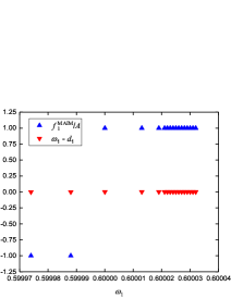
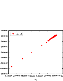
Fig. 1: Comparison of $\frac{f_{s}^{\mathrm{MAIM}}}{A}$ and $\omega-d_{s}$ for $d_{1}=0.6$ (left: full; right: zoomed).

3.4.2 Parametric study of the mapping functions

We can consider the WENO-JS scheme as a mapped WENO scheme with a mapping function defined as $\big{(}g^{\mathrm{JS}}\big{)}_{s}(\omega)=\omega$. Then, it can be easily verified that $\big{(}g^{\mathrm{MAIM}1}\big{)}_{s}(\omega)\big{\lvert}_{m_{s}\to 0}=\big{(}g^{\mathrm{JS}}\big{)}_{s}(\omega)$, $\big{(}g^{\mathrm{MAIM}5}\big{)}_{s}\big{(}\omega\big{)}\big{\lvert}_{k=2,A=1,C=1}=\big{(}g^{\mathrm{M}}\big{)}_{s}(\omega)$, $\big{(}g^{\mathrm{MAIM}5}\big{)}_{s}\big{(}\omega\big{)}\\ \big{\lvert}_{k=2,A=0.1,C=1}=\big{(}g^{\mathrm{IM}}\big{)}_{s}(\omega;2,0.1)$. We present these results directly in Fig.2(a). For $\big{(}g^{\mathrm{MAIM}1}\big{)}_{s}(\omega)$, we have the following properties: (1) for given $k$ and $A$, decreasing $m_{s}$ will make the function follow the identity map more closely but to narrow the optimal weight interval (see Fig.2(b)), and the optimal weight interval stands for the interval about $\omega=d_{s}$ over which the mapping process attempts to use the corresponding optimal weight; (2) for given $A$ and $m_{s}$, the optimal weight interval is widened by increasing $k$ as more derivatives vanish at $\omega=d_{s}$ (see Fig.2(c)); (3) for given $k$ and $m_{s}$, the optimal weight interval is narrowed by increasing $A$ (see Fig.2(d)).

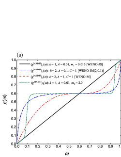
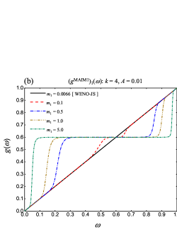
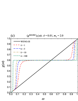
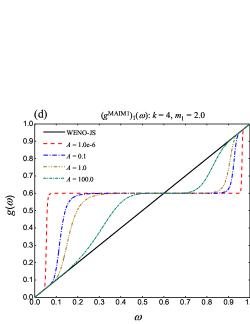
Fig. 2: New mapping functions $\big{(}g^{\mathrm{MAIM}1}\big{)}_{1}(\omega)$, $\big{(}g^{\mathrm{MAIM}5}\big{)}_{1}(\omega)$, and effect of varying parameters $k,A$ and $m_{s}$ on $\big{(}g^{\mathrm{MAIM}1}\big{)}_{1}(\omega)$ for $d_{1}=0.6$.

For $\big{(}g^{\mathrm{MAIM}2}\big{)}_{s}(\omega)$, it is trivial to show that $\big{(}g^{\mathrm{MAIM}2}\big{)}_{s}\big{(}\omega\big{)}\big{\lvert}_{k=1,A=0.01,Q=100,\mathrm{CFS}_{s}=1}=\big{(}g^{\mathrm{JS}}\big{)}_{s}(\omega)$, $\big{(}g^{\mathrm{MAIM}2}\big{)}_{s}\big{(}\omega\big{)}\big{\lvert}_{k=2,A=1,\mathrm{CFS}_{s}=0}\\ =\big{(}g^{\mathrm{M}}\big{)}_{s}(\omega)$, $\big{(}g^{\mathrm{MAIM}2}\big{)}_{s}\big{(}\omega\big{)}\big{\lvert}_{k=2,A=0.1,\mathrm{CFS}_{s}=0}=\big{(}g^{\mathrm{IM}}\big{)}_{s}(\omega;2,0.1)$. We illustrate these results directly in Fig.3(a). Similarly, for $\big{(}g^{\mathrm{MAIM}2}\big{)}_{s}(\omega)$, we have the following properties: (1) for given $k,A$ and $\mathrm{CFS}_{s}$, increasing $Q$ makes the function follow the identity map more closely and narrow the optimal weight interval down to the minimum optimal weight interval controlled by the parameter $\mathrm{CFS}_{s}$ (see Fig.3(b)); (2) for given $k,A$ and $Q$, the optimal weight interval is widened by decreasing $\mathrm{CFS}_{s}$ (see Fig.3(c)); (3) the effects of parameters $k$ and $A$ are the same as in $\big{(}g^{\mathrm{MAIM}1}\big{)}_{s}(\omega)$, but one must consider the effect of the parameter $\mathrm{CFS}_{s}$ (see Fig.3(d)).

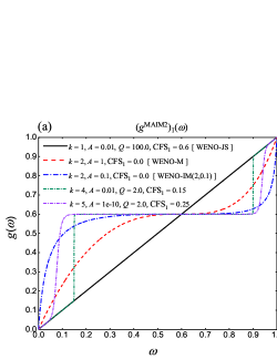
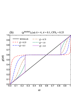
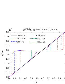
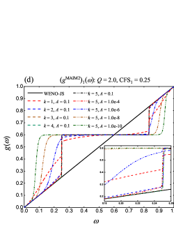
Fig. 3: Effect of varying parameters $k,A,Q$ and $\mathrm{CFS}_{s}$ on $\big{(}g^{\mathrm{MAIM}2}\big{)}_{1}(\omega)$ for $d_{1}=0.6$.

The study of the mapping functions $\big{(}g^{\mathrm{MAIM}3}\big{)}_{s}(\omega)$ and $\big{(}g^{\mathrm{MAIM}4}\big{)}_{s}(\omega)$ is slightly more complicated as these functions are not independent functions of $\omega$: one must obtain the relationship of $\big{(}g^{\mathrm{MAIM}3}\big{)}_{s}(\omega)\sim\omega$ or $\big{(}g^{\mathrm{MAIM}4}\big{)}_{s}(\omega)\sim\omega$ by specific numerical examples. We found that if the problem is non-smooth, these mapping functions will not maintain the monotonicity property. To illustrate this result, we take the linear advection equation $u_{t}+u_{x}=0$ as an example with the following initial condition consisting of two constant states separated by sharp discontinuities at $x=0,\pm 1$

$$u(x,0)=\left\{\begin{array}[]{ll}1,&x\in[-1,0),\\ 0,&x\in[0,1].\end{array}\right.$$ (19)

The results are shown in Fig.4 at the resolution $N=200$ cells and output time $t=200$. In the calculations, the CFL number is chosen to be $0.1$ and the periodic boundary conditions in two directions are used. From Fig.4, we see that the mapping functions $\big{(}g^{\mathrm{MAIM}3}\big{)}_{s}(\omega)$ and $\big{(}g^{\mathrm{MAIM}4}\big{)}_{s}(\omega)$ are non-monotonic with respect to $\omega$ for non-smooth problems. However, the monotonicity of the mapping functions $\big{(}g^{\mathrm{MAIM}1}\big{)}_{s}(\omega)$ and $\big{(}g^{\mathrm{MAIM}2}\big{)}_{s}(\omega)$ with respect to $\omega$ can be maintained very well.

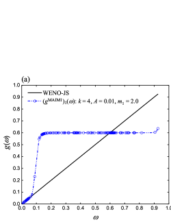
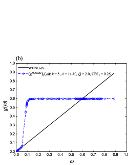
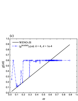
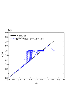
Fig. 4: Comparison of the mapping functions $\big{(}g^{\mathrm{MAIM}1}\big{)}_{1}(\omega)$, $\big{(}g^{\mathrm{MAIM}2}\big{)}_{1}(\omega)$, $\big{(}g^{\mathrm{MAIM}3}\big{)}_{1}(\omega)$, $\big{(}g^{\mathrm{MAIM}4}\big{)}_{1}(\omega)$ and $\big{(}g^{\mathrm{AIM}}\big{)}_{1}(\omega;4,2,1\mathrm{e}4)$ for $d_{1}=0.6$ for linear advection equation (18) with initial condition (19).

3.4.3 The rate of convergence

WENO schemes up to $17$th-order of accuracy have been outlined by Gerolymos et al. in [11]. Notationally, let $n_{\mathrm{cp}}\in\mathbb{N}$ denote the order of the critical point; that is, if $n_{\mathrm{cp}}=k_{\mathrm{crit}}$, then $f^{\prime}=\cdots=f^{(k_{\mathrm{crit}})}=0$ and $f^{(k_{\mathrm{crit}}+1)}\neq 0$. Now, we present Theorem 20, which will show that the WENO-MAIM$i$ schemes can recover the optimal convergence rates by setting the parameter $k$ for different values of $n_{\mathrm{cp}}$ in smooth regions.

Theorem 2

Let $\lceil x\rceil$ be a ceiling function of $x$, for $n_{\mathrm{cp}}<r-1$, the WENO-MAIM$i$ schemes can achieve the optimal $(2r-1)$th-order of accuracy if the modified adaptive improved mapping functions $(g^{\mathrm{MAIM}i})_{s}(\omega)$ defined in Eq.(15) are applied to the original weights in the WENO-JS scheme with $k\geq k^{\mathrm{MAIM}}$, where

$$k^{\mathrm{MAIM}}=\Bigg{\lceil}\dfrac{r}{r-1-n_{\mathrm{cp}}}-2\Bigg{\rceil}+\dfrac{1+\Big{(}-1\Big{)}^{\Bigg{\lceil}\dfrac{r}{r-1-n_{\mathrm{cp}}}-2\Bigg{\rceil}}}{2}.$$ (20)

Before giving the proof of Theorem 20, we state the following two lemmas.

Lemma 4

When $n_{\mathrm{cp}}<r-1$, the weights $\omega_{s}^{\mathrm{JS}}$ in the $(2r-1)$th-order WENO-JS scheme satisfy

$$\omega_{s}^{\mathrm{JS}}-d_{s}=O(\Delta x^{r-1-n_{\mathrm{cp}}}),\quad r=2,3,\cdots,9,$$ (21)

then, the convergence order is

$$r_{\mathrm{c}}=\left\{\begin{array}[]{ll}2r-1,&\mathrm{if}\quad n_{\mathrm{cp}}=0,\\ 2r-2-n_{\mathrm{cp}},&\mathrm{if}\quad n_{\mathrm{cp}}=1,2,\cdots,r-1.\end{array}\right.$$

The above lemma is a direct extension of Lemma 2 in [10], and we only extend the range of $r$ from $r=2,3,\cdots,6$ to $r=2,3,\cdots,9$. As the proof of the lemma can be found on page 565 in [18], we simply state it explicitly here.

Lemma 5

For $r=2,3,\cdots,9$, the sufficient condition for the $(2r-1)$ th-order WENO scheme to achieve the optimal order of accuracy is

$$\omega_{s}-d_{s}=O(\Delta x^{r}),\quad s=0,1,\cdots,r-1.$$

Remark 4

The proof of Lemma 5 in this paper is the finite volume version of Lemma 1 in [10], which is a natural extension of the one in [18]. For more details about the proof within the finite volume framework, the reference [35] is refered to.

Proof of Theorem 20.

(1) If $k=2n,n\in\mathbb{N}^{+}$, from Theorem 1, Corollary 1 and Corollary 2, we have $\big{(}g^{\mathrm{MAIM}i}\big{)}_{s}(d_{s})=d_{s}$ and $\big{(}g^{\mathrm{MAIM}i}\big{)}^{\prime}_{s}(d_{s})=\big{(}g^{\mathrm{MAIM}i}\big{)}^{\prime\prime}_{s}(d_{s})=\cdots=\big{(}g^{\mathrm{MAIM}i}\big{)}^{(k)}_{s}(d_{s})=0,\big{(}g^{\mathrm{MAIM}i}\big{)}^{(k+1)}_{s}(d_{s})\neq 0.$ Thus, evaluation at $\omega_{s}^{\mathrm{JS}}$ of the Taylor series approximation of the $\big{(}g^{\mathrm{MAIM}i}\big{)}_{s}(\omega)$ about $d_{s}$ yields

$$\alpha_{s}^{\mathrm{MAIM}i} =\big{(}g^{\mathrm{MAIM}i}\big{)}_{s}(d_{s})+\sum_{l=1}^{k}\dfrac{\big{(}g^{\mathrm{MAIM}i}\big{)}^{(l)}_{s}(d_{s})}{l!}\Big{(}\omega_{s}^{\mathrm{JS}}-d_{s}\Big{)}^{l}+\dfrac{\big{(}g^{\mathrm{MAIM}i}\big{)}^{(k+1)}_{s}(d_{s})}{(k+1)!}\Big{(}\omega_{s}^{\mathrm{JS}}-d_{s}\Big{)}^{k+1}+\cdots$$

$$=d_{s}+\dfrac{\big{(}g^{\mathrm{MAIM}i}\big{)}^{(k+1)}_{s}(d_{s})}{(k+1)!}\Big{(}\omega_{s}^{\mathrm{JS}}-d_{s}\Big{)}^{k+1}+\cdots$$

According to Lemma 4 and Lemma 5, the $(2r-1)$th-order WENO-MAIM$i$ schemes can achieve the optimal $(2r-1)$th-order of accuracy with requirement

$$(r-1-n_{\mathrm{cp}})(k+1)\geq r,\quad 1\leq n_{\mathrm{cp}}<r-1.$$

As $k=2n,n\in\mathbb{N}^{+}$, we can rewrite the requirement above as $k\geq k_{(2n)}^{\mathrm{MAIM}}$ by introducing

$$k_{(2n)}^{\mathrm{MAIM}}=\Bigg{\lceil}\dfrac{r}{r-1-n_{\mathrm{cp}}}-1\Bigg{\rceil}+\dfrac{1-\Big{(}-1\Big{)}^{\Bigg{\lceil}\dfrac{r}{r-1-n_{\mathrm{cp}}}-1\Bigg{\rceil}}}{2}.$$

(2) If $k=2n-1,n\in\mathbb{N}^{+}$, from Theorem 1, Corollary 1 and Corollary 2, we have $\big{(}g^{\mathrm{MAIM}i}\big{)}_{s}(d_{s})=d_{s}$ and $\big{(}g^{\mathrm{MAIM}i}\big{)}^{\prime}_{s}(d_{s})=\big{(}g^{\mathrm{MAIM}i}\big{)}^{\prime\prime}_{s}(d_{s})=\cdots=\big{(}g^{\mathrm{MAIM}i}\big{)}^{(k+1)}_{s}(d_{s})=0,\big{(}g^{\mathrm{MAIM}i}\big{)}^{(k+2)}_{s}(d_{s})\neq 0.$ Therefore, similarly, evaluation at $\omega_{s}^{\mathrm{JS}}$ of the Taylor series approximation of the $\big{(}g^{\mathrm{MAIM}i}\big{)}_{s}(\omega)$ about $d_{s}$ yields

$$\alpha_{s}^{\mathrm{MAIM}i} =\big{(}g^{\mathrm{MAIM}i}\big{)}_{s}(d_{s})+\sum_{l=1}^{k+1}\dfrac{\big{(}g^{\mathrm{MAIM}i}\big{)}^{(l)}_{s}(d_{s})}{l!}\Big{(}\omega_{s}^{\mathrm{JS}}-d_{s}\Big{)}^{l}+\dfrac{\big{(}g^{\mathrm{MAIM}i}\big{)}^{(k+2)}_{s}(d_{s})}{(k+2)!}\Big{(}\omega_{s}^{\mathrm{JS}}-d_{s}\Big{)}^{k+2}+\cdots$$

$$=d_{s}+\dfrac{\big{(}g^{\mathrm{MAIM}i}\big{)}^{(k+2)}_{s}(d_{s})}{(k+2)!}\Big{(}\omega_{s}^{\mathrm{JS}}-d_{s}\Big{)}^{k+2}+\cdots$$

Furthermore, according to Lemma 4 and Lemma 5, the $(2r-1)$th-order WENO-MAIM$i$ schemes can achieve the optimal $(2r-1)$th-order of accuracy with requirement

$$(r-1-n_{\mathrm{cp}})(k+2)\geq r,\quad 1\leq n_{\mathrm{cp}}<r-1.$$

As $k=2n-1,n\in\mathbb{N}^{+}$, we can rewrite the requirement above as $k\geq k_{(2n-1)}^{\mathrm{MAIM}}$ by introducing

$$k_{(2n-1)}^{\mathrm{MAIM}}=\Bigg{\lceil}\dfrac{r}{r-1-n_{\mathrm{cp}}}-2\Bigg{\rceil}+\dfrac{1+\Big{(}-1\Big{)}^{\Bigg{\lceil}\dfrac{r}{r-1-n_{\mathrm{cp}}}-2\Bigg{\rceil}}}{2}.$$

Clearly, we only need to ensure $k\geq k^{\mathrm{MAIM}}$, with $k^{\mathrm{MAIM}}=\min\Big{(}k_{(2n-1)}^{\mathrm{MAIM}},k_{(2n)}^{\mathrm{MAIM}}\Big{)}$, to achieve the optimal $(2r-1)$th-order of accuracy. It is easy to check that $k_{(2n-1)}^{\mathrm{MAIM}}\leq k_{(2n)}^{\mathrm{MAIM}}$. Eventually, we obtain

$$k^{\mathrm{MAIM}}=\Bigg{\lceil}\dfrac{r}{r-1-n_{\mathrm{cp}}}-2\Bigg{\rceil}+\dfrac{1+\Big{(}-1\Big{)}^{\Bigg{\lceil}\dfrac{r}{r-1-n_{\mathrm{cp}}}-2\Bigg{\rceil}}}{2}.$$ (22)

$\hfill\square$

Remark 5

For different values of $n_{\mathrm{cp}}$, we can calculate the detailed convergence order of the WENO-MAIM$i$ schemes using Theorem 20. Table 1 is a comparison between WENO-JS, WENO-M($1$), WENO-M($2$), WENO-IM($k,A$ ) and WENO-MAIM$i$. Note that WENO-M($n$) stands for WENO-M schemes with $n$ times mapping, and their rates of convergence are related to $r$ and $n_{\mathrm{cp}}$. A general conclusion of the rates of convergence of WENO-M($n$) schemes is proposed in Lemma 6, and we provide the proof in Appendix B.

Lemma 6

If $n$ mapping is used in the $(2r-1)$th-order WENO-M scheme, then for different values of $n_{\mathrm{cp}}$, the weights $\omega_{s}^{\mathrm{M}}$ in the $(2r-1)$th-order WENO-M scheme satisfy

$$\omega_{s}^{\mathrm{M}}-d_{s}=O\Big{(}(\Delta x)^{3^{n}\times(r-1-n_{\mathrm{cp}})}\Big{)},\quad r=2,3,\cdots,9,\quad n_{\mathrm{cp}}=0,1,\cdots,r-1,$$

and the rate of convergence is

$$r_{\mathrm{c}}=\left\{\begin{array}[]{ll}2r-1,&\mathrm{if}\quad n_{\mathrm{cp}}=0,\cdots,\Bigg{\lfloor}\dfrac{3^{n}-1}{3^{n}}r-1\Bigg{\rfloor},\\ (3^{n}+1)(r-1)-3^{n}\times n_{\mathrm{cp}},&\mathrm{if}\quad n_{\mathrm{cp}}=\Bigg{\lfloor}\dfrac{3^{n}-1}{3^{n}}r-1\Bigg{\rfloor}+1,\cdots,r-1.\end{array}\right.$$

where $\lfloor x\rfloor$ is a floor function of $x$.

4 Numerical experiments

In this section, we present the results of the modified adaptive improved mapped WENO-MAIM$i$ schemes in comparison with the WENO-JS, WENO-M and WENO-IM($2,0.1$) schemes, and all these schemes are in the finite volume version with $\epsilon=10^{-40}$. The global Lax-Friedrichs numerical flux is used in the following numerical experiments. The $L_{1}$-, $L_{2}$- and $L_{\infty}$- norm of the error are calculated by comparing the numerical solution $(u_{h})_{j}$ with the exact solution $u_{j}^{\mathrm{exact}}$ according to

$$\begin{array}[]{l}L_{1}(h)=\displaystyle\sum\limits_{j}h\cdot\big{\lvert}u_{j}^{\mathrm{exact}}-(u_{h})_{j}\big{\rvert},\\ L_{2}(h)=\sqrt{\displaystyle\sum\limits_{j}h\cdot\big{(}u_{j}^{\mathrm{exact}}-(u_{h})_{j}\big{)}^{2}},\\ L_{\infty}(h)=\max\limits_{j}\big{\lvert}u_{j}^{\mathrm{exact}}-(u_{h})_{j}\big{\rvert},\end{array}$$

where $h=\Delta x$ is the spatial step size.

We focus on the performance of the fifth-order WENO-MAIM$1$($10,1\mathrm{e-}6,0.06$), WENO-MAIM$2$($2,0.1,10,1\mathrm{e-}6$), WENO-MAIM$3$($10,1\mathrm{e-}6$) and WENO-MAIM$4$($1.0,1\mathrm{e-}6$) schemes. Without causing any confusion, we denote these four schemes as WENO-MAIM$1$, WENO-MAIM$2$, WENO-MAIM$3$ and WENO-MAIM$4$ for simplicity. Notably, the main purpose for choosing the specific WENO-MAIM$2$ scheme here is to verify the conclusion in subsection 3.4.2 that WENO-MAIM$2$($k,A,Q,0$) = WENO-IM($k,A$), through numerical examples. We show that for all the following examples, the WENO-MAIM$2$ scheme provides exactly the same results as those of the WENO-IM($2,0.1$) scheme.

Table 1: Convergence orders for the WENO-JS, WENO-M(1), WENO-M(2), WENO-IM($k,A$) and WENO-MAIM$i$ schemes.

	$n_{\mathrm{cp}}$	$r_{\mathrm{c}}$-WENO-JS	$r_{\mathrm{c}}$-WENO-M($1$)	$r_{\mathrm{c}}$-WENO-M($2$)	$r_{\mathrm{c}}$ -WENO-IM($k,A$)	$r_{\mathrm{c}}$-WENO-MAIM$i$
$r=2$	$0$	$3$	$3$	$3$	$3(k\geq 2)$	$3(k\geq 1)$
	$1$	$1$	$1$	$1$	$1$	$1$
$r=3$	$0$	$5$	$5$	$5$	$5(k\geq 2)$	$5(k\geq 1)$
	$1$	$3$	$5$	$5$	$5(k\geq 2)$	$5(k\geq 1)$
	$2$	$2$	$2$	$2$	$2$	$2$
$r=4$	$0$	$7$	$7$	$7$	$7(k\geq 2)$	$7(k\geq 1)$
	$1$	$5$	$7$	$7$	$7(k\geq 2)$	$7(k\geq 1)$
	$2$	$4$	$6$	$7$	$7(k\geq 4)$	$7(k\geq 3)$
	$3$	$3$	$3$	$3$	$3$	$3$
$r=5$	$0$	$9$	$9$	$9$	$9(k\geq 2)$	$9(k\geq 1)$
	$1$	$7$	$9$	$9$	$9(k\geq 2)$	$9(k\geq 1)$
	$2$	$6$	$9$	$9$	$9(k\geq 2)$	$9(k\geq 1)$
	$3$	$5$	$7$	$9$	$9(k\geq 4)$	$9(k\geq 3)$
	$4$	$4$	$4$	$4$	$4$	$4$
$r=6$	$0$	$11$	$11$	$11$	$11(k\geq 2)$	$11(k\geq 1)$
	$1$	$9$	$11$	$11$	$11(k\geq 2)$	$11(k\geq 1)$
	$2$	$8$	$11$	$11$	$11(k\geq 2)$	$11(k\geq 1)$
	$3$	$7$	$11$	$11$	$11(k\geq 2)$	$11(k\geq 1)$
	$4$	$6$	$8$	$11$	$11(k\geq 6)$	$11(k\geq 5)$
	$5$	$5$	$5$	$5$	$5$	$5$
$r=7$	$0$	$13$	$13$	$13$	$13(k\geq 2)$	$13(k\geq 1)$
	$1$	$11$	$13$	$13$	$13(k\geq 2)$	$13(k\geq 1)$
	$2$	$10$	$13$	$13$	$13(k\geq 2)$	$13(k\geq 1)$
	$3$	$9$	$13$	$13$	$13(k\geq 2)$	$13(k\geq 1)$
	$4$	$8$	$12$	$13$	$13(k\geq 4)$	$13(k\geq 3)$
	$5$	$7$	$9$	$13$	$13(k\geq 6)$	$13(k\geq 5)$
	$6$	$6$	$6$	$6$	$6$	$6$
$r=8$	$0$	$15$	$15$	$15$	$15(k\geq 2)$	$15(k\geq 1)$
	$1$	$13$	$15$	$15$	$15(k\geq 2)$	$15(k\geq 1)$
	$2$	$12$	$15$	$15$	$15(k\geq 2)$	$15(k\geq 1)$
	$3$	$11$	$15$	$15$	$15(k\geq 2)$	$15(k\geq 1)$
	$4$	$10$	$15$	$15$	$15(k\geq 2)$	$15(k\geq 1)$
	$5$	$9$	$13$	$15$	$15(k\geq 4)$	$15(k\geq 3)$
	$6$	$8$	$10$	$15$	$15(k\geq 8)$	$15(k\geq 7)$
	$7$	$7$	$7$	$7$	$7$	$7$
$r=9$	$0$	$17$	$17$	$17$	$17(k\geq 2)$	$17(k\geq 1)$
	$1$	$15$	$17$	$17$	$17(k\geq 2)$	$17(k\geq 1)$
	$2$	$14$	$17$	$17$	$17(k\geq 2)$	$17(k\geq 1)$
	$3$	$13$	$17$	$17$	$17(k\geq 2)$	$17(k\geq 1)$
	$4$	$12$	$17$	$17$	$17(k\geq 2)$	$17(k\geq 1)$
	$5$	$11$	$17$	$17$	$17(k\geq 2)$	$17(k\geq 1)$
	$6$	$10$	$14$	$17$	$17(k\geq 4)$	$17(k\geq 3)$
	$7$	$9$	$11$	$17$	$17(k\geq 8)$	$17(k\geq 7)$
	$8$	$8$	$8$	$8$	$8$	$8$

4.1 Accuracy test

Example 1

(Accuracy test without any critical points [10]) We solve the one-dimensional linear advection equation $u_{t}+u_{x}=0$ with the following initial condition

$$u(x,0)=\sin(\pi x)$$ (23)

and the periodic boundary conditions. Note that we consider only the fifth-order methods here, and to ensure that the error for the overall scheme is a measure of the spatial convergence only, we set the CFL number to be $(\Delta x)^{2/3}$. Clearly, the initial condition in (23) has no critical points.

Table 2 shows the errors and convergence rates (in brackets, hereinafter the same) for the numerical solutions of Example 1 produced by various schemes at output time $t=2.0$. The results of the three rows are $L_{1}$-, $L_{2}$- and $L_{\infty}$- norm errors and orders in turn (the same below). All the schemes achieve close to their designed order of accuracy. In terms of accuracy, the WENO-MAIM$1$, WENO-MAIM$2$, WENO-MAIM$3$ and WENO-MAIM$4$ schemes provide almost equally accurate numerical solutions as the WENO-M and WENO-IM($2,0.1$) schemes, which provide more accurate numerical solutions than the WENO-JS scheme.

Table 2: Convergence properties of various schemes solving $u_{t}+u_{x}=0$ with initial condition $u(x,0)=\sin(\pi x)$.

$N$	$20$	$40$	$80$	$160$	$320$
WENO-JS	2.96529e-03(-)	9.27609e-05(4.9985)	2.89265e-06(5.0031)	9.03392e-08(5.0009)	2.82330e-09(4.9999)
	2.42673e-03(-)	7.64322e-05(4.9887)	2.33581e-06(5.0322)	7.19259e-08(5.0213)	2.23105e-09(5.0107)
	2.57899e-03(-)	9.05453e-05(4.8320)	2.90709e-06(4.9610)	8.85753e-08(5.0365)	2.72458e-09(5.0228)
WENO-M	5.18291e-04(-)	1.59422e-05(5.0288)	4.98914e-07(4.9979)	1.56021e-08(4.9990)	4.88356e-10(4.9977)
	4.06148e-04(-)	1.25236e-05(5.0193)	3.91875e-07(4.9981)	1.22541e-08(4.9991)	3.83568e-10(4.9976)
	3.94913e-04(-)	1.24993e-05(4.9816)	3.91808e-07(4.9956)	1.22538e-08(4.9988)	3.83541e-10(4.9977)
WENO-IM(2,0.1)	5.04401e-04(-)	1.59160e-05(4.9860)	4.98863e-07(4.9957)	1.56020e-08(4.9988)	4.88355e-10(4.9977)
	3.96236e-04(-)	1.25033e-05(4.9860)	4.98863e-07(4.6475)	1.22541e-08(5.3473)	3.83568e-10(4.9976)
	3.94458e-04(-)	1.24963e-05(4.9803)	3.91797e-07(4.9953)	1.22538e-08(4.9988)	3.83547e-10(4.9977)
WENO-MAIM1	5.08205e-04(-)	1.59130e-05(4.9971)	4.98858e-07(4.9954)	1.56020e-08(4.9988)	4.88355e-10(4.9977)
	4.26155e-04(-)	1.25010e-05(5.0913)	3.91831e-07(4.9957)	1.22541e-08(4.9989)	3.83568e-10(4.9976)
	5.03701e-04(-)	1.24960e-05(5.3330)	3.91795e-07(4.9952)	1.22538e-08(4.9988)	3.83543e-10(4.9977)
WENO-MAIM2	5.04401e-04(-)	1.59160e-05(4.9860)	4.98863e-07(4.9957)	1.56020e-08(4.9988)	4.88355e-10(4.9977)
	3.96236e-04(-)	1.25033e-05(4.9860)	4.98863e-07(4.6475)	1.22541e-08(5.3473)	3.83568e-10(4.9976)
	3.94458e-04(-)	1.24963e-05(4.9803)	3.91797e-07(4.9953)	1.22538e-08(4.9988)	3.83547e-10(4.9977)
WENO-MAIM3	5.02844e-04(-)	1.59130e-05(4.9818)	4.98858e-07(4.9954)	1.56020e-08(4.9988)	4.88355e-10(4.9977)
	3.95138e-04(-)	1.25010e-05(4.9822)	3.91831e-07(4.9957)	1.22541e-08(4.9989)	3.83568e-10(4.9976)
	3.94406e-04(-)	1.24960e-05(4.9801)	3.91795e-07(4.9952)	1.22538e-08(4.9988)	3.83543e-10(4.9977)
WENO-MAIM4	5.02845e-04(-)	1.59131e-05(4.9818)	4.98858e-07(4.9954)	1.56020e-08(4.9988)	4.88355e-10(4.9977)
	3.95139e-04(-)	1.25010e-05(4.9822)	3.91831e-07(4.9957)	1.22541e-08(4.9989)	3.83568e-10(4.9976)
	3.94406e-04(-)	1.24960e-05(4.9801)	3.91795e-074.9952	1.22538e-08(4.9988)	3.83540e-10(4.9977)

Example 2

(Accuracy test with first-order critical points [18]) We solve the one-dimensional linear advection equation $u_{t}+u_{x}=0$ with the following initial condition

$$u(x,0)=\sin\bigg{(}\pi x-\dfrac{\sin(\pi x)}{\pi}\bigg{)}$$ (24)

and periodic boundary conditions. Again, the CFL number is set to be $(\Delta x)^{2/3}$. It is easy to verify that the particular initial condition in (24) has two first-order critical points, which both have a non-vanishing third derivative.

The errors and convergence rates for the numerical solutions of Example 2 produced by various schemes at output time $t=2.0$ are shown in Table 3. We can observe that the WENO-MAIM$1$, WENO-MAIM$2$, WENO-MAIM$3$ and WENO-MAIM$4$ schemes maintain the fifth-order convergence rate even in the presence of critical points. Moreover, in terms of accuracy, these four WENO schemes provide the equally accurate results as the WENO-M and WENO-IM($2,0.1$) schemes, and are much more accurate than the WENO-JS scheme, whose errors are much larger and the convergence rates are lower than fifth-order.

Table 3: Convergence properties of various schemes solving $u_{t}+u_{x}=0$ with initial condition $u(x,0)=\sin(\pi x-\sin(\pi x)/\pi)$.

$N$	$20$	$40$	$80$	$160$	$320$
WENO-JS	1.01260e-02(-)	7.22169e-04(3.8096)	3.42286e-05(4.3991)	1.58510e-06(4.4326)	7.95517e-08(4.3165)
	8.72198e-03(-)	6.76133e-04(3.6893)	3.63761e-05(4.2162)	2.29598e-06(3.9858)	1.68304e-07(3.7700)
	1.43499e-02(-)	1.09663e-03(3.7099)	9.02485e-05(3.6030)	8.24022e-06(3.4531)	8.31702e-07(3.3085)
WENO-M	3.70838e-03(-)	1.45082e-04(4.6758)	4.80253e-06(4.9169)	1.52120e-07(4.9805)	4.77083e-09(4.9948)
	3.36224e-03(-)	1.39007e-04(4.5962)	4.52646e-06(4.9406)	1.42463e-07(4.9897)	4.45822e-09(4.9980)
	5.43666e-03(-)	2.18799e-04(4.6350)	6.81451e-06(5.0049)	2.14545e-07(4.9893)	6.71080e-09(4.9987)
WENO-IM(2,0.1)	4.30725e-03(-)	1.51327e-04(4.8310)	4.85592e-06(4.9618)	1.52659e-07(4.9914)	4.77654e-09(4.9982)
	3.93700e-03(-)	1.41737e-04(4.7958)	4.53602e-06(4.9656)	1.42479e-07(4.9926)	4.45805e-09(4.9982)
	5.84039e-03(-)	2.10531e-04(4.7940)	6.82606e-06(4.9468)	2.14534e-07(4.9918)	6.71079e-09(4.9986)
WENO-MAIM1	8.07923e-03(-)	3.32483e-04(4.6029)	1.01162e-05(5.0385)	1.52910e-07(6.0478)	4.77728e-09(5.0003)
	7.08117e-03(-)	3.36264e-04(4.3963)	1.49724e-05(4.4892)	1.42515e-07(6.7150)	4.45807e-09(4.9986)
	1.03772e-02(-)	6.62891e-04(3.9685)	4.48554e-05(3.8854)	2.14522e-07(7.7080)	6.71079e-09(4.9985)
WENO-MAIM2	4.30725e-03(-)	1.51327e-04(4.8310)	4.85592e-06(4.9618)	1.52659e-07(4.9914)	4.77654e-09(4.9982)
	3.93700e-03(-)	1.41737e-04(4.7958)	4.53602e-06(4.9656)	1.42479e-07(4.9926)	4.45805e-09(4.9982)
	5.84039e-03(-)	2.10531e-04(4.7940)	6.82606e-06(4.9468)	2.14534e-07(4.9918)	6.71079e-09(4.9986)
WENO-MAIM3	4.39527e-03(-)	1.52219e-04(4.8517)	4.86436e-06(4.9678)	1.52735e-07(4.9931)	4.77728e-09(4.9987)
	4.02909e-03(-)	1.42172e-04(4.8247)	4.53770e-06(4.9695)	1.42486e-07(4.9931)	4.45807e-09(4.9983)
	5.89045e-03(-)	2.09893e-04(4.8107)	6.83017e-06(4.9416)	2.14533e-07(4.9926)	6.71079e-09(4.9986)
WENO-MAIM4	4.94421e-03(-)	1.52224e-04(5.0215)	4.86436e-06(4.9678)	1.52735e-07(4.9931)	4.77728e-09(4.9987)
	4.50651e-03(-)	1.42174e-04(4.9863)	4.53770e-06(4.9696)	1.42486e-07(4.9931)	4.45807e-09(4.9983)
	6.56976e-03(-)	2.09893e-04(4.9681)	6.83018e-06(4.9416)	2.14533e-07(4.9927)	6.71079e-09(4.9986)

4.2 Performance on calculating linear advection examples with discontinuities at long output times

After extensive numerical tests, we find that the WENO-MAIM3 and WENO-MAIM4 schemes have a significant advantage that they not only can obtain high resolution, but also can prevent generating spurious oscillations on calculating linear advection problems with discontinuities when the output time is large. However, the other considered schemes do not have this advantage. To demonstrate this, we apply the considered schemes to one-dimensional linear advection equation $u_{t}+u_{x}=0$ with the following two initial conditions on uniform grid sizes and at long output times.

Case 1. (SLP) The initial condition is given by

$$\begin{array}[]{l}u(x,0)=\left\{\begin{array}[]{ll}\dfrac{1}{6}\big{[}G(x,\beta,z-\hat{\delta})+4G(x,\beta,z)+G(x,\beta,z+\hat{\delta})\big{]},&x\in[-0.8,-0.6],\\ 1,&x\in[-0.4,-0.2],\\ 1-\big{\lvert}10(x-0.1)\big{\rvert},&x\in[0.0,0.2],\\ \dfrac{1}{6}\big{[}F(x,\alpha,a-\hat{\delta})+4F(x,\alpha,a)+F(x,\alpha,a+\hat{\delta})\big{]},&x\in[0.4,0.6],\\ 0,&\mathrm{otherwise},\end{array}\right.\end{array}$$ (25)

where $G(x,\beta,z)=\mathrm{e}^{-\beta(x-z)^{2}},F(x,\alpha,a)=\sqrt{\max\big{(}1-\alpha^{2}(x-a)^{2},0\big{)}}$, and the constants $z=-0.7,\hat{\delta}=0.005,\beta=\dfrac{\log 2}{36\hat{\delta}^{2}},a=0.5$ and $\alpha=10$.

Case 2. (BiCWP) The initial condition is given by

$$\begin{array}[]{l}u(x,0)=\left\{\begin{array}[]{ll}0,&x\in[-1.0,-0.8]\bigcup(-0.2,0.2]\bigcup(0.8,1.0],\\ 0.5,&x\in(-0.6,-0.4]\bigcup(0.2,0.4]\bigcup(0.6,0.8],\\ 1,&x\in(-0.8,-0.6]\bigcup(-0.4,-0.2]\bigcup(0.4,0.6].\end{array}\right.\end{array}$$ (26)

The periodic boundary condition is used in the two directions and the CFL number is set to be $0.1$ for both Case 1 and Case 2. Case 1 consists of a Gaussian, a square wave, a sharp triangle and a semi-ellipse, and Case 2 consists of several constant states separated by sharp discontinuities at $x=\pm 0.8,\pm 0.6,\pm 0.4,\pm 0.2$. For simplicity, we call Case 1 SLP as it is a Linear Problem first proposed by Shu et al. in [20], and we call Case 2 BiCWP as the profile of the exact solution for this Problem looks like the Breach in City Wall.

Firstly, we calculate both SLP and BiCWP by all considered WENO schemes using the uniform grid sizes of $N=200,400,800$ with a long output time $t=2000$. Table 4 has shown the errors and convergence rates, and we find that: (1) in terms of accuracy, when solving SLP, the WENO-MAIM3 scheme provides the most accurate solutions among all considered WENO schemes at $N=200,400,800$, and when solving BiCWP, the WENO-MAIM3 and WENO-MAIM4 schemes provide more accurate solutions than other considered WENO schemes at $N=800$; (2) as expected, the WENO-MAIM$i(i=1,2,3,4)$ schemes, as well as the WENO-IM(2, 0.1) scheme, show more accurate solutions than the WENO-JS and WENO-M schemes on solving both SLP and BiCWP; (3) in terms of convergence rates, the $L_{1}$ and $L_{2}$ orders of the WENO-MAIM$i(i=1,2,3,4)$ and WENO-IM(2, 0.1) schemes are significantly higher than those of the WENO-JS and WENO-M schemes; (4) furthermore, on solutions of SLP, the $L_{1}$ and $L_{2}$ orders of the WENO-MAIM$i(i=1,2,3,4)$ and WENO-IM(2, 0.1) schemes are approximately $1.0$ and $0.5\sim 0.7$ respectively, and their $L_{\infty}$ orders are all positive; (5) on solutions of BiCWP, the $L_{1}$ orders are also approximately $1.0$ for the WENO-MAIM1, WENO-MAIM3 and WENO-MAIM4 schemes while only about $0.8$ for the WENO-IM(2, 0.1) and WENO-MAIM2 schemes, and the $L_{2}$ orders are about $0.45$ for the WENO-MAIM1, WENO-MAIM3 and WENO-MAIM4 schemes while slightly lower with the value of about $0.4$ for the WENO-IM(2, 0.1) and WENO-MAIM2 schemes; (6) on solutions of BiCWP, the $L_{\infty}$ orders become negative for the WENO-IM(2, 0.1), WENO-MAIM1 and WENO-MAIM2 schemes while maintain positive for the WENO-MAIM3 and WENO-MAIM4 schemes.

Fig. 5 and Fig. 6 have shown the comparisons of various schemes on solving SLP and BiCWP when $t=2000$ and $N=800$. We can observe that: (1) when solving SLP, the WENO-MAIM3 and WENO-MAIM4 schemes do not generate spurious oscillations and provide the numerical results with a significantly higher resolution than those of the WENO-JS and WENO-M schemes; (2) in general, the WENO-MAIM1, WENO-MAIM2 and WENO-IM(2, 0.1) schemes also show very high resolution and almost do not generate spurious oscillations when solving SLP, but if we take a closer look, we can see that the WENO-MAIM2 and WENO-IM(2, 0.1) schemes give a significantly lower resolution of the Gaussian (see Fig. 5(b)) and a slightly lower resolution of the square wave near $x=-0.16$ (see Fig. 5(d)) than the WENO-MAIM1, WENO-MAIM3 and WENO-MAIM4 schemes; (3) furthermore, the WENO-MAIM2 and WENO-IM(2, 0.1) schemes generate a very slight spurious oscillation, which is hard to be noticed without a very close look, around the square wave near $x=-0.435$ (see Fig. 5(c)), while the other considered schemes do not generate this spurious oscillation; (4) when solving BiCWP, the spurious oscillations generated by the WENO-IM(2, 0.1), WENO-MAIM1 and WENO-MAIM2 schemes become very evident, while the WENO-MAIM3 and WENO-MAIM4 schemes still provide the numerical results with much sharper resolutions than those of the WENO-JS and WENO-M schemes but do not produce spurious oscillations.

Table 4: Convergence properties of various schemes solving SLP and BiCWP at output time $t=2000$.

	SLP			BiCWP
$N$	$200$	$400$	$800$	$200$	$400$	$800$
WENO-JS	6.12899e-01(-)	5.99215e-01(0.0326)	5.50158e-01 (0.1232)	5.89672e-01(-)	5.56639e-01(0.0832)	4.72439e-01 (0.2366)
	5.08726e-01(-)	5.01160e-01(0.0216)	4.67585e-01 (0.1000)	4.70933e-01(-)	4.41787e-01(0.0922)	3.78432e-01 (0.2233)
	7.99265e-01(-)	8.20493e-01(-0.0378)	8.14650e-01 (0.0103)	6.41175e-01(-)	5.94616e-01(0.1088)	5.73614e-01 (0.0519)
WENO-M	3.81597e-01(-)	3.25323e-01(0.2302)	3.48528e-01 (-0.0994)	3.27647e-01(-)	2.64334e-01(0.3098)	2.57390e-01 (0.0384)
	3.59205e-01(-)	3.12970e-01(0.1988)	3.24373e-01 (-0.0516)	2.73948e-01(-)	2.60726e-01(0.0714)	2.47361e-01 (0.0759)
	6.89414e-01(-)	6.75473e-01(0.0295)	6.25645e-01 (0.1106)	5.12247e-01(-)	5.60199e-01(-0.1291)	5.83690e-01 (-0.0593)
WENO-IM(2,0.1)	2.17411e-01(-)	1.12590e-01(0.9493)	5.18367e-02 (1.1190)	1.96196e-01(-)	1.12264e-01(0.8054)	6.48339e-02 (0.7921)
	2.30000e-01(-)	1.64458e-01(0.4839)	9.98968e-02 (0.7192)	2.07227e-01(-)	1.54544e-01(0.4232)	1.16534e-01 (0.4073)
	5.69864e-01(-)	4.82180e-01(0.2410)	4.73102e-01 (0.0274)	4.98939e-01(-)	4.68309e-01(0.0914)	4.91291e-01 (-0.0691)
WENO-MAIM1	2.18238e-01(-)	1.09902e-01(0.9897)	4.41601e-02 (1.3154)	2.04996e-01(-)	1.33104e-01(0.6230)	6.77607e-02 (0.9740)
	2.29151e-01(-)	1.51024e-01(0.6015)	9.35506e-02 (0.6910)	2.07725e-01(-)	1.62892e-01(0.3508)	1.18338e-01 (0.4610)
	5.63682e-01(-)	4.94657e-01(0.1885)	4.72393e-01 (0.0664)	4.93792e-01(-)	4.96724e-01(-0.0085)	5.13570e-01 (-0.0481)
WENO-MAIM2	2.17411e-01(-)	1.12590e-01(0.9493)	5.18367e-02 (1.1190)	1.96196e-01(-)	1.12264e-01(0.8054)	6.48339e-02 (0.7921)
	2.30000e-01(-)	1.64458e-01(0.4839)	9.98968e-02 (0.7192)	2.07227e-01(-)	1.54544e-01(0.4232)	1.16534e-01 (0.4073)
	5.69864e-01(-)	4.82180e-01(0.2410)	4.73102e-01 (0.0274)	4.98939e-01(-)	4.68309e-01(0.0914)	4.91291e-01 (-0.0691)
WENO-MAIM3	2.17339e-01(-)	9.91687e-02(1.1320)	4.37214e-02 (1.1815)	1.78226e-01(-)	1.19271e-01(0.5795)	6.25800e-02 (0.9305)
	2.28723e-01(-)	1.45461e-01(0.6530)	9.31160e-02 (0.6435)	1.97298e-01(-)	1.57392e-01(0.3260)	1.15580e-01 (0.4455)
	5.63600e-01(-)	4.79774e-01(0.2323)	4.71185e-01 (0.0261)	5.01513e-01(-)	4.75377e-01(0.0772)	4.71183e-01 (0.0128)
WENO-MAIM4	2.18548e-01(-)	1.03499e-01(1.0783)	4.39609e-02 (1.2353)	2.05283e-01(-)	1.28349e-01(0.6775)	6.33284e-02 (1.0191)
	2.30043e-01(-)	1.48300e-01(0.6334)	9.34567e-02 (0.6661)	2.07890e-01(-)	1.60928e-01(0.3694)	1.16112e-01 (0.4709)
	5.65659e-01(-)	4.91295e-01(0.2033)	4.71240e-01 (0.0601)	4.90417e-01(-)	4.89146e-01(0.0037)	4.71240e-01 (0.0538)

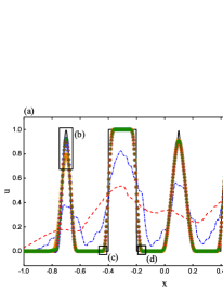
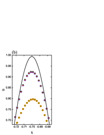
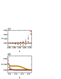
Fig. 5: Performance of the fifth-order WENO-JS, WENO-M, WENO-IM($2,0.1$) and WENO-MAIM$i$($i=1,2,3,4$) schemes for the SLP with $N=800$ at long output time $t=2000$.

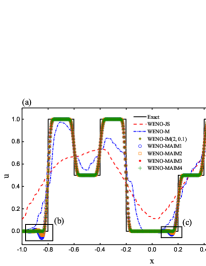
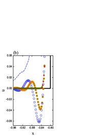
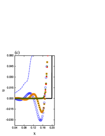
Fig. 6: Performance of the fifth-order WENO-JS, WENO-M, WENO-IM($2,0.1$) and WENO-MAIM$i$($i=1,2,3,4$) schemes for the BiCWP with $N=800$ at long output time $t=2000$.

In addition, we calculate both SLP and BiCWP with a shortened but still long output time $t=200$ and larger uniform grid sizes of $N=1600,3200,6400$. Table 5 has shown the errors and convergence rates, and we find that: (1) in terms of accuracy, the WENO-JS and WENO-M schemes generate less accurate solutions than other considered WENO schemes as expected; (2) the WENO-MAIM3 scheme provides the most accurate solutions among all considered WENO schemes at $N=1600,3200,6400$ on solving SLP, and it also provides the most accurate solutions at $N=3200,6400$ on solving BiCWP; (3) when solving both SLP and BiCWP, the WENO-MAIM4 scheme gives more accurate solutions than other consider WENO schemes except the WENO-MAIM3 scheme at $N=6400$; (4) in terms of convergence rates, the $L_{1}$ and $L_{2}$ orders of the WENO-MAIM$i(i=1,2,3,4)$ and WENO-IM(2, 0.1) schemes are higher than those of the WENO-JS and WENO-M schemes in general; (5) on solutions of SLP, the $L_{1}$ and $L_{2}$ orders are approximately $0.88$ and $0.42$ respectively for the WENO-MAIM1, WENO-MAIM3 and WENO-MAIM4 schemes, while slightly lower with the values about $0.83$ and $0.40$ respectively for the WENO-IM(2, 0.1) and WENO-MAIM2 schemes; (6) similarly, on solutions of BiCWP, the $L_{1}$ and $L_{2}$ orders are approximately $0.83$ and $0.42$ respectively for the WENO-MAIM1, WENO-MAIM3 and WENO-MAIM4 schemes, while slightly lower with the values about $0.80$ and $0.41$ respectively for the WENO-IM(2, 0.1) and WENO-MAIM2 schemes; (7) on solutions of both SLP and BiCWP, the $L_{\infty}$ orders of the WENO-MAIM$i(1,2,3,4)$ and WENO-IM(2, 0.1) schemes are all negative, but the absolute values of the $L_{\infty}$ orders of the WENO-MAIM3 and WENO-MAIM4 schemes are smaller than those of the WENO-IM(2, 0.1), WENO-MAIM1 and WENO-MAIM2 schemes.

In Figs.7, 8, 9 and Figs.10, 11, 12, we have shown the comparison of various schemes when $t=200$ and $N=1600,3200,6400$ for SLP and BiCWP respectively. We observe that: (1) when solving SLP, as the grid number increases, the WENO-MAIM1, WENO-MAIM2 and WENO-IM(2, 0.1) schemes generate evident spurious oscillations, while the WENO-MAIM3 and WENO-MAIM4 schemes do not but provide improved resolutions; (2) although the WENO-JS and WENO-M schemes obtain numerical results with improved resolutions for both SLP and BiCWP when the grid number increases, their resolutions are significantly lower than those of the WENO-MAIM3 and WENO-MAIM4 schemes; (3) for both SLP and BiCWP, when the grid number increases, the spurious oscillations of the WENO-IM(2, 0.1), WENO-MAIM1 and WENO-MAIM2 schemes get closer to the discontinuities, and the amplitudes of these spurious oscillations become larger; (4) however, the solutions of the WENO-MAIM3 and WENO-MAIM4 schemes get closer to the exact solutions without generating spurious oscillations.

Table 5: Convergence properties of various schemes solving SLP and BiCWP at output time $t=200$.

	SLP			BiCWP
$N$	$1600$	$3200$	$6400$	$1600$	$3200$	$6400$
WENO-JS	1.26804e-01(-)	8.81339e-02(0.5248)	6.14430e-02 (0.5204)	1.47671e-01(-)	1.15707e-01(0.3519)	8.55015e-02 (0.4365)
	1.67490e-01(-)	1.37054e-01(0.2893)	1.10915e-01 (0.3053)	1.78065e-01(-)	1.56061e-01(0.1903)	1.32873e-01 (0.2321)
	5.17972e-01(-)	5.17039e-01(0.0026)	5.07030e-01 (0.0282)	5.28594e-01(-)	5.35169e-01(-0.0275)	5.13562e-01 (0.0595)
WENO-M	4.21095e-02(-)	3.13290e-02(0.4266)	2.89979e-02 (0.1116)	4.45182e-02(-)	4.70277e-02(-0.0791)	5.36042e-02 (-0.1888)
	8.47168e-02(-)	8.10687e-02(0.0635)	8.58473e-02 (-0.0826)	9.35523e-02(-)	1.01968e-01(-0.1243)	1.09394e-01 (-0.1014)
	5.06850e-01(-)	6.10861e-01(-0.2693)	5.04121e-01 (0.2771)	5.06372e-01(-)	5.71919e-01(-0.1756)	5.04359e-01 (0.1814)
WENO-IM(2,0.1)	1.26519e-02(-)	6.56498e-03(0.9465)	3.68884e-03 (0.8316)	2.39427e-02(-)	1.35781e-02(0.8183)	7.78055e-03 (0.8033)
	5.48733e-02(-)	4.08544e-02(0.4256)	3.08433e-02 (0.4055)	7.14167e-02(-)	5.35510e-02(0.4153)	4.03989e-02 (0.4066)
	4.62587e-01(-)	4.69803e-01(-0.0223)	4.87134e-01 (-0.0523)	4.62587e-01(-)	4.69803e-01(-0.0223)	4.87134e-01 (-0.0523)
WENO-MAIM1	1.35847e-02(-)	7.18556e-03(0.9188)	3.93600e-03 (0.8684)	2.55329e-02(-)	1.44669e-02(0.8196)	8.15452e-03 (0.8271)
	5.64038e-02(-)	4.20972e-02(0.4221)	3.14976e-02 (0.4185)	7.29915e-02(-)	5.48110e-02(0.4133)	4.10730e-02 (0.4163)
	4.82675e-01(-)	4.98673e-01(-0.0470)	5.10410e-01 (-0.0336)	4.82672e-01(-)	4.98672e-01(-0.0470)	5.10411e-01 (-0.0336)
WENO-MAIM2	1.26519e-02(-)	6.56498e-03(0.9465)	3.68884e-03 (0.8316)	2.39427e-02(-)	1.35781e-02(0.8183)	7.78055e-03 (0.8033)
	5.48733e-02(-)	4.08544e-02(0.4256)	3.08433e-02 (0.4055)	7.14167e-02(-)	5.35510e-02(0.4153)	4.03989e-02 (0.4066)
	4.62587e-01(-)	4.69803e-01(-0.0223)	4.87134e-01 (-0.0523)	4.62587e-01(-)	4.69803e-01(-0.0223)	4.87134e-01 (-0.0523)
WENO-MAIM3	1.23903e-02(-)	6.43177e-03(0.9459)	3.49736e-03 (0.8789)	2.39789e-02(-)	1.34355e-02(0.8357)	7.53547e-03 (0.8343)
	5.48637e-02(-)	4.08071e-02(0.4270)	3.05283e-02 (0.4187)	7.14302e-02(-)	5.35161e-02(0.4166)	4.01067e-02 (0.4161)
	4.62409e-01(-)	4.66452e-01(-0.0126)	4.70087e-01 (-0.0112)	4.62408e-01(-)	4.66453e-01(-0.0126)	4.70087e-01 (-0.0112)
WENO-MAIM4	1.23934e-02(-)	6.53848e-03(0.9225)	3.54066e-03 (0.8849)	2.44954e-02(-)	1.36623e-02(0.8423)	7.63475e-03 (0.8395)
	5.53035e-02(-)	4.10626e-02(0.4295)	3.06775e-02 (0.4206)	7.19931e-02(-)	5.38487e-02(0.4189)	4.03025e-02 (0.4180)
	4.62634e-01(-)	4.66590e-01(-0.0123)	4.70166e-01 (-0.0110)	4.62641e-01(-)	4.66590e-01(-0.0123)	4.70166e-01 (-0.0110)

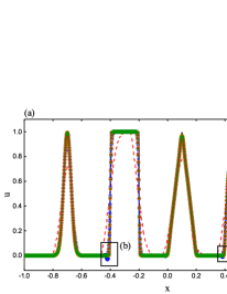
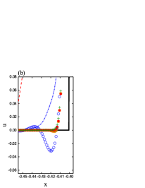
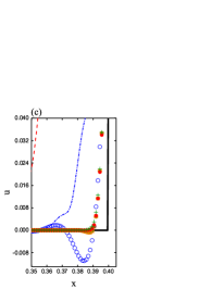
Fig. 7: Performance of the fifth-order WENO-JS, WENO-M, WENO-IM($2,0.1$) and WENO-MAIM$i$($i=1,2,3,4$) schemes for the SLP with $N=1600$ at long output time $t=200$.

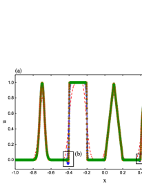
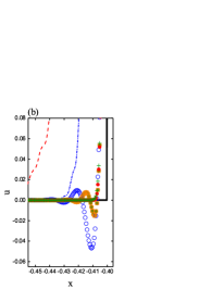
Fig. 8: Performance of the fifth-order WENO-JS, WENO-M, WENO-IM($2,0.1$) and WENO-MAIM$i$($i=1,2,3,4$) schemes for the SLP with $N=3200$ at long output time $t=200$.

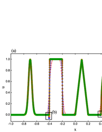
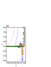
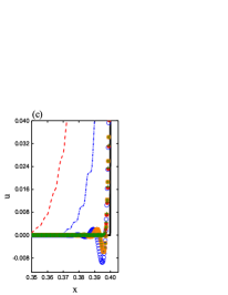
Fig. 9: Performance of the fifth-order WENO-JS, WENO-M, WENO-IM($2,0.1$) and WENO-MAIM$i$($i=1,2,3,4$) schemes for the SLP with $N=6400$ at long output time $t=200$.

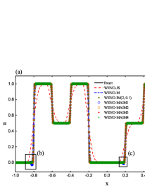
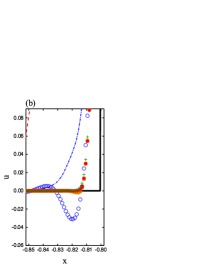
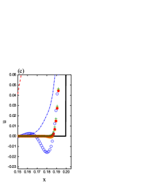
Fig. 10: Performance of the fifth-order WENO-JS, WENO-M, WENO-IM($2,0.1$) and WENO-MAIM$i$($i=1,2,3,4$) schemes for the BiCWP with $N=1600$ at long output time $t=200$.

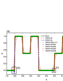
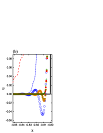
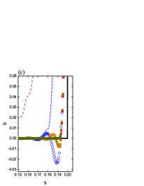
Fig. 11: Performance of the fifth-order WENO-JS, WENO-M, WENO-IM($2,0.1$) and WENO-MAIM$i$($i=1,2,3,4$) schemes for the BiCWP with $N=3200$ at long output time $t=200$.

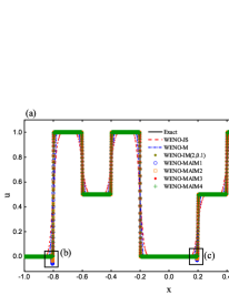
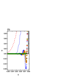
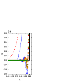
Fig. 12: Performance of the fifth-order WENO-JS, WENO-M, WENO-IM($2,0.1$) and WENO-MAIM$i$($i=1,2,3,4$) schemes for the BiCWP with $N=6400$ at long output time $t=200$.

4.3 One-dimensional Euler system

In this subsection, we present numerical examples of the one-dimensional Euler system for gas dynamics in the following conservation form with different initial and boundary conditions

$$\mathbf{U}_{t}+\mathbf{F}\big{(}\mathbf{U}\big{)}_{x}=0,$$ (27)

where $\mathbf{U}=\big{(}\rho,\rho u,E\big{)}^{\mathrm{T}},\mathbf{F}\big{(}\mathbf{U}\big{)}=\big{(}\rho u,\rho u^{2}+p,u(E+p)\big{)}^{\mathrm{T}}$, and $\rho,u,p$ and $E$ are the density, velocity, pressure and total energy, respectively. The Euler system (27) is closed by the equation of state for an ideal polytropic gas, which is given by

$$p=(\gamma-1)\Big{(}E-\dfrac{1}{2}\rho u^{2}\Big{)},\quad\gamma=1.4$$

The finite volume version of the characteristic-wise one-dimensional WENO procedure is employed, and we refer to [27] for details. In all calculations of this subsection, the CFL number is set to be $0.1$ and the reference solutions are obtained by using the WENO-JS scheme with the resolution of $N=10000$.

Example 3

(Woodward-Colella interacting blast wave problem) We solve the one-dimensional blast waves interaction problem of Woodward and Colella [34], which has the following initial condition with reflective boundary conditions

$$\big{(}\rho,u,p\big{)}(x,0)=\left\{\begin{array}[]{ll}(1,0,1000),&x\in[0,0.1),\\ (1,0,0.01),&x\in[0.1,0.9),\\ (1,0,100),&x\in[0.9,1.0].\end{array}\right.$$ (28)

This problem is run with $N=400$ uniform cells till $t=0.038$ by the WENO-JS, WENO-M, WENO-IM($2,0.1$) and WENO-MAIM$i$($i=1,2,3,4$) schemes.

Surprisingly, for this specific problem, the WENO-MAIM2 and WENO-IM($2,0.1$) schemes blow up in our calculations, but the other schemes perform well. The results are given in Fig. 13. It can be observed directly from Fig. 13 that the WENO-MAIM$3$ scheme provides the best performance, followed by the WENO-MAIM4 scheme and then the WENO-M scheme. The WENO-MAIM$1$ scheme performs worse than most of the considered schemes but slightly better than the WENO-JS scheme.

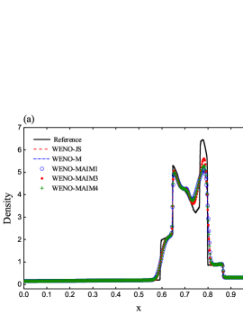
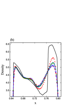
Fig. 13: Performance of fifth-order WENO-JS, WENO-M and WENO-MAIM$i$ ($i=1,3,4$) for Euler system (27) with initial condition (28).

Example 4

(Titarev-Toro shock-entropy wave interaction problem) We solve the one-dimensional shock-entropy wave interaction problem proposed by Titarev and Toro [30, 32, 31] which is a more severe version of the classic Shu-Osher shock-entropy wave interaction problem [29]. This example is commonly used to test the ability to capture both shocks and short wavelength oscillations of the numerical schemes, and the amplitudes of the short wavelength oscillations are a measure of the numerical viscosity of the schemes. The initial condition is given by

$$\big{(}\rho,u,p\big{)}(x,0)=\left\{\begin{array}[]{ll}(1.515695,0.5233346,1.80500),&x\in[-5.0,-4.5],\\ (1.0+0.1\sin(20\pi x),0,1),&x\in[-4.5,5.0].\end{array}\right.$$ (29)

It is run with $N=1500$ uniform cells till $t=5.0$ and the CFL number is set to be $0.4$.

The results are shown in Fig. 14. It can be seen that the WENO-MAIM3 scheme results in slightly greater amplitudes compared to the WENO-MAIM2, WENO-MAIM4 and WENO-IM($2,0.1$) schemes which produce higher amplitudes of the short wavelength oscillations compared to the WENO-M scheme. The WENO-MAIM1 scheme performs slightly better than the WENO-JS scheme which performs worst among all the considered WENO schemes for this case.

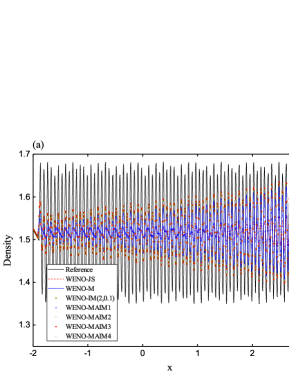
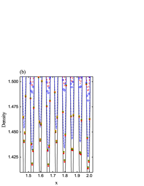
Fig. 14: Performance of fifth-order WENO-JS, WENO-M, WENO-IM($2,0.1$ ) and WENO-MAIM$i$($i=1,2,3,4$) for Euler system (27) with initial condition (29).

4.4 Two-dimensional Euler system

In this subsection, we extend the considered WENO schemes to calculate the two-dimensional compressible Euler system of gas dynamics taking the following strong conservation form

$$\mathbf{U}_{t}+\mathbf{F}\big{(}\mathbf{U}\big{)}_{x}+\mathbf{G}\big{(}\mathbf{U}\big{)}_{y}=0,$$ (30)

where $\mathbf{U}=\big{(}\rho,\rho u,\rho v,E\big{)}^{\mathrm{T}},\mathbf{F}\big{(}\mathbf{U}\big{)}=\big{(}\rho u,\rho u^{2}+p,\rho uv,u(E+p)\big{)}^{\mathrm{T}},\mathbf{G}\big{(}\mathbf{U}\big{)}=\big{(}\rho v,\rho vu,\rho v^{2}+p,v(E+p)\big{)}^{\mathrm{T}}$, and $\rho,u,v,p$ and $E$ are the density, component of velocity in the $x$ and $y$ coordinate directions, pressure and total energy, respectively. The Euler system (30) is closed by the equation of state for an ideal polytropic gas given by

$$p=(\gamma-1)\Big{(}E-\dfrac{1}{2}\rho(u^{2}+v^{2})\Big{)},\quad\gamma=1.4$$

In all numerical examples of this subsection, the CFL number is set to be $0.5$. As the WENO-MAIM2 scheme gives exactly the same solutions as the WENO-IM(2, 0.1) scheme, we only show the results of the WENO-IM(2, 0.1) scheme for brevity in the following presentation.

Example 5

(2D Riemann problem) We calculate the 2D Riemann problem proposed by [26, 25]. This problem is done over a unit square domain $[0,1]\times[0,1]$. There are many different configurations for 2D Riemann problem [25], and we focus on the one solved in [22, 25]. It initially involves the constant states of flow variables over each quadrant which is got by dividing the computational domain using lines $x=0.5$ and $y=0.5$. The initial constant states are given by

$$\big{(}\rho,u,v,p\big{)}(x,y,0)=\left\{\begin{aligned} \begin{array}[]{ll}(1.0,0.0,-0.3,1.0),&0.5\leq x\leq 1.0,0.5\leq y\leq 1.0,\\ (2.0,0.0,0.3,1.0),&0.0\leq x\leq 0.5,0.5\leq y\leq 1.0,\\ (1.0625,0.0,0.8145,0.4),&0.0\leq x\leq 0.5,0.0\leq y\leq 0.5,\\ (0.5313,0.0,0.4276,0.4),&0.5\leq x\leq 1.0,0.0\leq y\leq 0.5.\\ \end{array}\end{aligned}\right.$$

The transmission boundary condition is used on all boundaries. We evolve the initial data until time $t=0.3$ using considered WENO schemes with a uniform mesh size of $1200\times 1200$.

The numerical results of density obtained using the WENO-JS, WENO-M, WENO-IM(2, 0.1), WENO-MAIM1, WENO-MAIM3 and WENO-MAIM4 schemes have been shown in Fig. 15. All these considered WENO schemes can captured the main structure of the solution. Furthermore, as mentioned in [22, 24], this example is commonly focused on the description of the instability of the slip line (marked by the pink dashed box in the first figure of Fig. 15). Thus, we have displayed the close-up view of this instability in Fig. 16. We can see that the WENO-JS, WENO-M and WENO-MAIM1 schemes failed to resolve the instability of the slip line under current spatial resolution. The WENO-IM(2, 0.1) scheme is able to resolve this instability, but it is not very noticeable. However, the structure of the instability in the solution of the WENO-MAIM3 scheme is evidently larger in size and has more waves when compared with that of the WENO-IM(2, 0.1) scheme, and this demonstrates the advantage of the WENO-MAIM3 scheme that has the lower dissipation and hence has a higher resolution in capturing details of the complicated flow structures. The solution of the WENO-MAIM4 scheme appears to resolve the instability with the waves larger in size but less in number than that of the WENO-IM(2, 0.1) scheme.

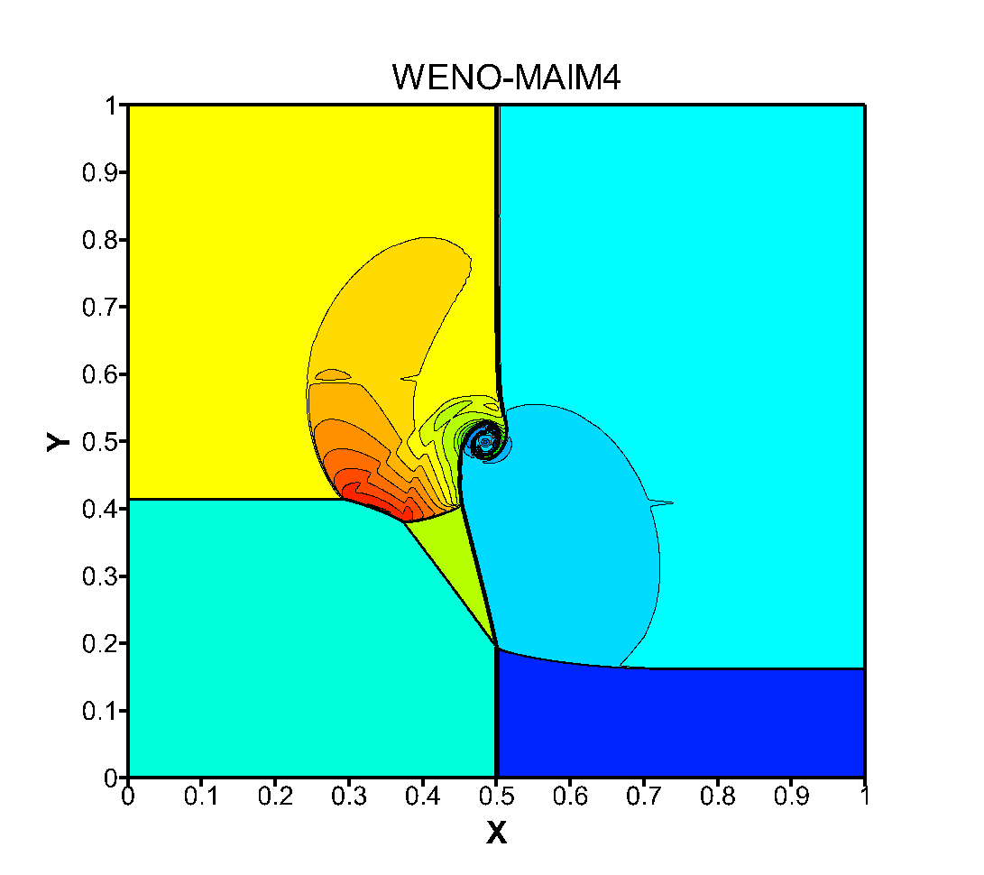
Fig. 15: Density plots for the 2D Riemann problem using $30$ contour lines with range from $0.5$ to $2.4$, computed using the WENO-JS, WENO-M, WENO-MAIM$i(i=1,2,3,4)$ schemes at output time $t=0.3$ with a uniform mesh size of $1200\times 1200$.

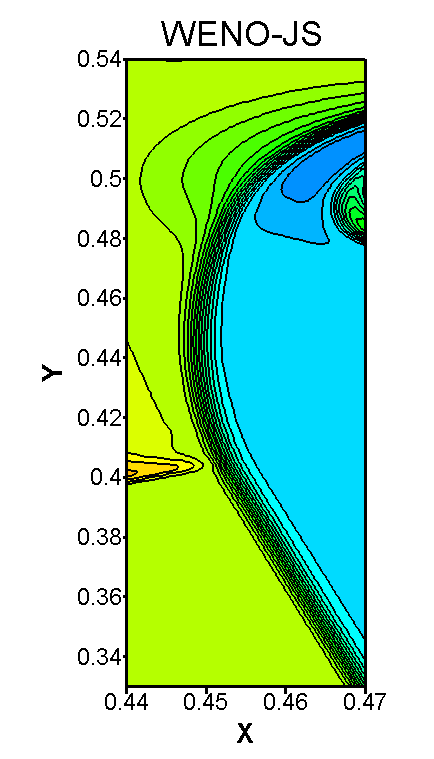
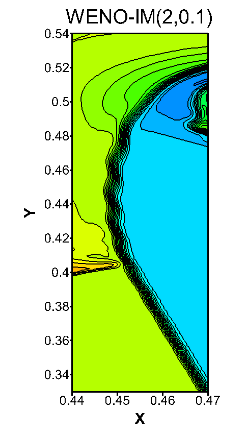
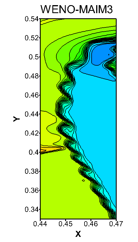
Fig. 16: The zoomed-in density plots for the 2D Riemann problem.

Example 6

(Double Mach reflection, DMR) We solve the two dimensional double Mach reflection problem [34] using the considered WENO schemes. It is a commonly used test where a vertical shock wave moves horizontally into a wedge that is inclined by some angle. The computational domain is $[0,4]\times[0,1]$ and the initial condition is given by

$$\big{(}\rho,u,v,p\big{)}(x,y,0)=\left\{\begin{aligned} \begin{array}[]{ll}(8.0,8.25\cos\dfrac{\pi}{6},-8.25\sin\dfrac{\pi}{6},116.5),&x<x_{0}+\dfrac{y}{\sqrt{3}},\\ (1.4,0.0,0.0,1.0),&x\geq x_{0}+\dfrac{y}{\sqrt{3}},\\ \end{array}\end{aligned}\right.$$

where $x_{0}=\frac{1}{6}$. At $x=0,4$, the inflow boundary condition with the post-shock values as stated above and the outflow boundary condition are used respectively. At $y=0$, the reflective boundary condition is applied to the interval $[x_{0},4]$, while at $(0,x_{0})$, the post-shock values are imposed. The boundary condition on the upper boundary $y=1$ is implemented as follows

$$\begin{array}[]{l}\big{(}\rho,u,v,p\big{)}(x,1,t)=\left\{\begin{array}[]{ll}(8.0,8.25\cos\dfrac{\pi}{6},-8.25\sin\dfrac{\pi}{6},116.5),&x\in[0,s(t)),\\ (1.4,0.0,0.0,1.0),&x\in[s(t),4].\end{array}\right.\end{array}$$

where $s(t)=x_{0}+\frac{1+20t}{\sqrt{3}}$ and it is the position of shock wave at time $t$ on the upper boundary. We discretize the computational domain using a uniform mesh size of $2000\times 500$ and the output time is set to be $t=0.2$.

As the instability of the slip line and the companion structures after the primary reflection shock (marked by the pink dashed box and the pink solid box in the first figure of Fig. 17 respectively) are the usual two concerns in this problem, we give the zoomed-in contours around the double Mach reflection region in Fig. 17. All the considered schemes can present the main structure of the double Mach reflection in general, and they can also successfully capture the companion structures behind the lower half of the right moving reflection shock. However, one can distinguish the dissipation of the various schemes by the number and size of the small vortices generated along the slip lines. It is clear that the WENO-MAIM3 scheme captures most in number and biggest in size of the small vortices. We can also see that all the mapped WENO schemes capture more in number and bigger in size of the small vortices than the WENO-JS scheme. The WENO-MAIM4 and WENO-IM(2, 0.1) schemes appear to give slightly better flow features near the slip lines than the WENO-MAIM1 and WENO-M schemes.

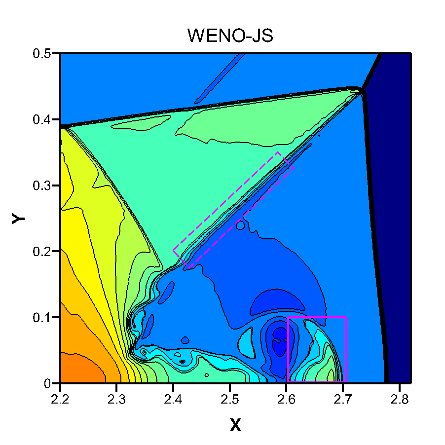
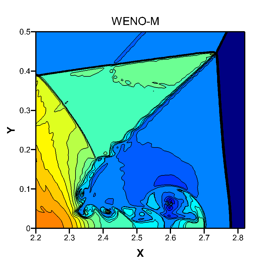
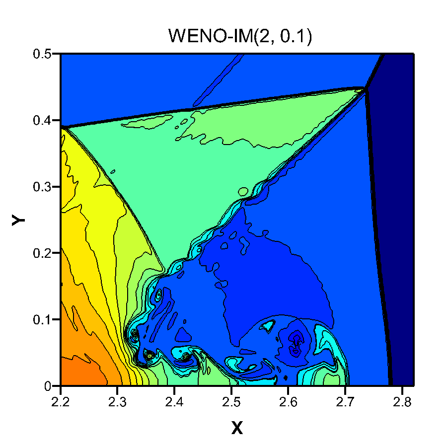
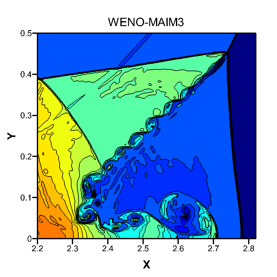
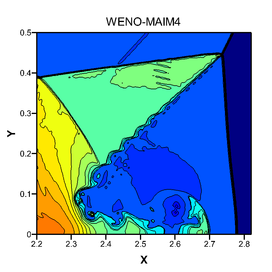
Fig. 17: Close-up views of performance of the WENO-JS, WENO-M, WENO-IM(2, 0.1) and WENO-MAIM$i(i=1,3,4)$ schemes for the DMR problem at output time $t=0.2$ with a uniform mesh size of $2000\times 500$.

Example 7

(Forward facing step problem, FFS) We solve the forward facing step problem first presented by Woodward and Colella [34]. Recently, some important details, like the physical instability and roll-up of the vortex sheet emanating from the Mach stem, have been successfully captured by various high order schemes [6, 2, 3, 8, 36]. We will show that our new method is also able to successfully capture these important details.

The setup of this problem is as follows: a step with a height of $0.2$ length units locates $0.6$ length units from the left-hand end of a wind tunnel that is $1$ length unit wide and $3$ length units long. The initial condition is specified by

$$\big{(}\rho,u,v,p\big{)}(x,y,0)=(1.4,3.0,0.0,1.0),\quad(x,y)\in\Omega.$$

where $\Omega=[0,0.6]\times[0,1]\cup[0.6,3]\times[0.2,1]$ is the computational domain. The reflective boundary condition is used along the walls of the wind tunnel and the step, and the inflow and outflow conditions are used at the entrance and the exit of the wind tunnel respectively. We discretize the computational domain using a uniform mesh size of $900\times 300$ and evolve the initial data until time $t=4$.

In Fig. 18, we have shown the density contours computed by considered WENO schemes. We can see that the considered schemes capture all the shocks properly with sharp profiles. Moreover, the roll-up of the vortex sheet in the solutions of the WENO-MAIM3 scheme is most visible, and this demonstrates the ability of the WENO-MAIM3 scheme to provide a better resolution in solving problems with complicated flow structures. We can see that the WENO-IM(2, 0.1) scheme also shows evidence of the vortex sheet’s roll-up although it is less evident than that of the WENO-MAIM3 scheme. Meanwhile, the vortex sheet’s roll-up is not observed in the solutions of the WENO-JS, WENO-M, WENO-MAIM1 and WENO-MAIM4 schemes.

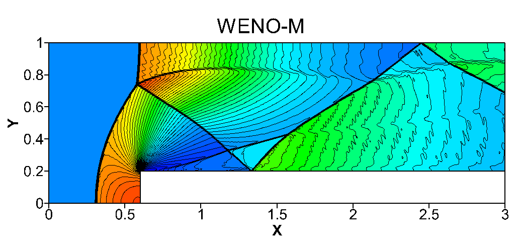
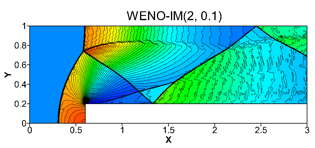
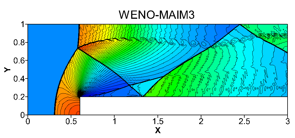
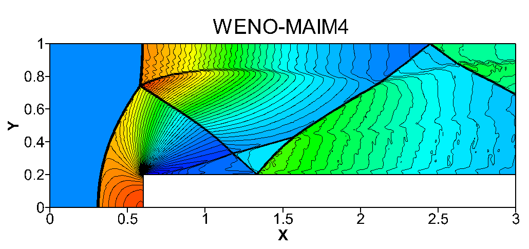
Fig. 18: Density plots for the forward facing step problem using 50 density contour lines with range from $0.32$ to $6.5$, computed using the WENO-JS, WENO-M, WENO-IM(2, 0.1) and WENO-MAIM$i(i=1,3,4)$ schemes at output time $t=4.0$ with a uniform mesh size of $900\times 300$.

5 Conclusions

We have devised a modified adaptive improved mapped WENO method, that is, WENO-MAIMi, by employing a new family of mapping functions. The new mapping functions are based on some adaptive control functions and a smoothing approximation of the signum function. This helps to introduce the adaptive nature and provide a wider selection of the parameters in the schemes. In several numerical experiments, one-dimensional scalar, as well as one- and two-dimensional system cases, is considered to show the performance of our new method. Four specified WENO-MAIM$i$ schemes with fine-tuned parameters are used, and all these proposed schemes can achieve optimal convergence orders even near critical points in smooth regions. When a short time simulation is desired, all the four proposed WENO-MAIM$i$ schemes are good choices in most hyperbolic conservation simulations. In summary, we recommend to use the WENO-MAIM$3$ scheme with parameters as $k=10$, $A=1\mathrm{e-}6$ for pratical computation, because it exhibits improved comprehensive performance in most hyperbolic conservation simulations. It shows clear advantages on approximating near discontinuities, especially for one-dimensional linear advection cases with long output time and two-dimensional cases with complicated solution structures.

Appendix A

The objective of this appendix is to present the results of the zero points of $q_{s}^{\prime}(\omega)$, the monotone intervals and maximum values of $q_{s}(\omega)$ in $\omega\in(0,1)$, and the recommended values of $\alpha_{s}$ in Property 3 and Property 4.

Table 6: The results of the zero points of $q_{s}^{\prime}(\omega)$, the monotone intervals and maximum values of $q_{s}(\omega)$ in $\omega\in(0,1)$, and the recommended values of $\alpha_{s}$ in Property 3 and Property 4.

$r$	$s$	$d_{s}$	$\omega_{\mathrm{crit}}$	$q_{s}^{\prime}(\omega)$			$q_{\mathrm{max}}(\omega)$	recommended value of $\alpha_{s}$
				$\omega\in(0,\omega_{\mathrm{crit}})$	$\omega=\omega_{\mathrm{crit}}$	$\omega\in(\omega_{\mathrm{crit}},1)$
$1$	$0$	$1$	-	$>0$	$>0$	$>0$	$<0$	$0.0001$
$2$	$0$	$1/3$	$0.380873415$	$>0$	$=0$	$<0$	$0.092362764$	$0.0924$
	$1$	$2/3$	$0.619126585$	$>0$	$=0$	$<0$	$0.092362764$	$0.0924$
$3$	$0$	$1/10$	$0.156515839$	$>0$	$=0$	$<0$	$0.574903653$	$0.5750$
	$1$	$6/10$	$0.570057856$	$>0$	$=0$	$<0$	$0.033129692$	$0.0332$
	$2$	$3/10$	$0.354983613$	$>0$	$=0$	$<0$	$0.133395837$	$0.1334$
$4$	$0$	$1/35$	$0.050334141$	$>0$	$=0$	$<0$	$0.954367890$	$0.9544$
	$1$	$12/35$	$0.388078022$	$>0$	$=0$	$<0$	$0.082052483$	$0.0821$
	$2$	$18/35$	$0.509902230$	$>0$	$=0$	$<0$	$0.000674949$	$0.0007$
	$3$	$4/35$	$0.174716514$	$>0$	$=0$	$<0$	$0.527277883$	$0.5273$
$5$	$0$	$1/126$	$0.014533733$	$>0$	$=0$	$<0$	$1.289877215$	$1.2899$
	$1$	$10/63$	$0.226106436$	$>0$	$=0$	$<0$	$0.401303129$	$0.4014$
	$2$	$10/21$	$0.483489850$	$>0$	$=0$	$<0$	$0.001874973$	$0.0019$
	$3$	$20/63$	$0.368684520$	$>0$	$=0$	$<0$	$0.110936397$	$0.1110$
	$4$	$5/126$	$0.068631349$	$>0$	$=0$	$<0$	$0.862927630$	$0.8630$
$6$	$0$	$1/462$	$0.004036768$	$>0$	$=0$	$<0$	$1.617654227$	$1.6177$
	$1$	$5/77$	$0.107726908$	$>0$	$=0$	$<0$	$0.716954249$	$0.7170$
	$2$	$25/77$	$0.374254393$	$>0$	$=0$	$<0$	$0.102277562$	$0.1023$
	$3$	$100/231$	$0.453273191$	$>0$	$=0$	$<0$	$0.014901369$	$0.0150$
	$4$	$25/154$	$0.229973747$	$>0$	$=0$	$<0$	$0.392223085$	$0.3923$
	$5$	$1/77$	$0.023524596$	$>0$	$=0$	$<0$	$1.163386235$	$1.1634$
$7$	$0$	$1/1716$	$0.001099119$	$>0$	$=0$	$<0$	$1.945668808$	$1.9457$
	$1$	$7/286$	$0.043419023$	$>0$	$=0$	$<0$	$0.996333645$	$0.9964$
	$2$	$105/572$	$0.251943992$	$>0$	$=0$	$<0$	$0.341617878$	$0.3417$
	$3$	$175/429$	$0.435602337$	$>0$	$=0$	$<0$	$0.028078584$	$0.0281$
	$4$	$175/572$	$0.359684813$	$>0$	$=0$	$<0$	$0.125509465$	$0.1256$
	$5$	$21/286$	$0.120110409$	$>0$	$=0$	$<0$	$0.678155990$	$0.6782$
	$6$	$7/1716$	$0.007550349$	$>0$	$=0$	$<0$	$1.458456912$	$1.4585$
$8$	$0$	$1/6435$	$0.000295439$	$>0$	$=0$	$<0$	$2.275453190$	$2.2755$
	$1$	$56/6435$	$0.015907656$	$>0$	$=0$	$<0$	$1.266360740$	$1.2664$
	$2$	$196/2145$	$0.145076866$	$>0$	$=0$	$<0$	$0.605994603$	$0.6060$
	$3$	$392/1287$	$0.358612853$	$>0$	$=0$	$<0$	$0.127291552$	$0.1273$
	$4$	$490/1287$	$0.416050440$	$>0$	$=0$	$<0$	$0.047165647$	$0.0472$
	$5$	$392/2145$	$0.251123145$	$>0$	$=0$	$<0$	$0.343478122$	$0.3435$
	$6$	$196/6435$	$0.053489044$	$>0$	$=0$	$<0$	$0.936837253$	$0.9369$
	$7$	$8/6435$	$0.002330913$	$>0$	$=0$	$<0$	$1.756424091$	$1.7565$
$9$	$0$	$1/24310$	$0.000078677$	$>0$	$=0$	$<0$	$2.607051525$	$2.6071$
	$1$	$36/12155$	$0.005504277$	$>0$	$=0$	$<0$	$2.607051528$	$2.6071$
	$2$	$504/12155$	$0.071503078$	$>0$	$=0$	$<0$	$0.850403988$	$0.8505$
	$3$	$2352/12155$	$0.261799125$	$>0$	$=0$	$<0$	$0.319476358$	$0.3195$
	$4$	$882/2431$	$0.402941270$	$>0$	$=0$	$<0$	$0.062457658$	$0.0625$
	$5$	$3528/12155$	$0.347184466$	$>0$	$=0$	$<0$	$0.146872875$	$0.1469$
	$6$	$1176/12155$	$0.152246813$	$>0$	$=0$	$<0$	$0.586388730$	$0.5864$
	$7$	$144/12155$	$0.021508966$	$>0$	$=0$	$<0$	$1.187147894$	$1.1872$
	$8$	$9/24310$	$0.000700372$	$>0$	$=0$	$<0$	$2.058883535$	$2.0589$

Appendix B

In this appendix, we present the proof of Lemma 6.

Proof of Lemma 6.

First, by employing the mapping function Eq.(6), the mapped weights with $n$ times mapping are given by

$$\omega_{s}^{\mathrm{M}(n)}=\dfrac{\alpha_{s}^{\mathrm{M}(n)}}{\sum_{l=0}^{r-1}\alpha_{l}^{\mathrm{M}(n)}},\alpha_{s}^{\mathrm{M}(n)}=\big{(}g^{\mathrm{M}}\big{)}_{s}(\omega^{\mathrm{M}(n-1)}_{s}),\quad s=0,1,\cdots,r-1,$$

where $\omega^{\mathrm{M}(n-1)}_{s}$ are the mapped weights with $n-1$ times mapping. Clearly, the mapped weights with $0$ times mapping are determined by

$$\omega^{\mathrm{M}(0)}_{s}=\omega_{s}^{\mathrm{JS}},$$ (31)

which are computed by Eq.(5). Similarly, as $\Big{(}g^{\mathrm{M}}\Big{)}_{s}(d_{s})=d_{s}$ and $\Big{(}g^{\mathrm{M}}\Big{)}^{\prime}_{s}(d_{s})=\Big{(}g^{\mathrm{M}}\Big{)}^{\prime\prime}_{s}(d_{s})=0,\big{(}g^{\mathrm{M}}\big{)}^{\prime\prime\prime}_{s}(d_{s})\neq 0$ in the WENO-M scheme, evaluation at $\omega_{s}^{\mathrm{M}(n-1)}$ of the Taylor series approximations of $\Big{(}g^{\mathrm{M}}\Big{)}_{s}(\omega)$ about $d_{s}$ yields

$$\alpha_{s}^{\mathrm{M}(n)} =\big{(}g^{\mathrm{M}}\big{)}_{s}(d_{s})+\big{(}g^{\mathrm{M}}\big{)}^{\prime}_{s}(d_{s})\Big{(}\omega_{s}^{\mathrm{M}(n-1)}-d_{s}\Big{)}+\dfrac{\big{(}g^{\mathrm{M}}\big{)}^{\prime\prime}_{s}(d_{s})}{2!}\Big{(}\omega_{s}^{\mathrm{M}(n-1)}-d_{s}\Big{)}^{2}+\dfrac{\big{(}g^{\mathrm{M}}\big{)}^{\prime\prime\prime}_{s}(d_{s})}{3!}\Big{(}\omega_{s}^{\mathrm{M}(n-1)}-d_{s}\Big{)}^{3}+\cdots$$

$$=d_{s}+\dfrac{\big{(}g^{\mathrm{M}}\big{)}^{\prime\prime\prime}_{s}(d_{s})}{3!}\Big{(}\omega_{s}^{\mathrm{M}(n-1)}-d_{s}\Big{)}^{3}+\cdots$$

By employing the fact that $\sum_{s=0}^{r-1}d_{s}=1$, we obtain

$$\dfrac{1}{\sum_{l=0}^{r-1}\alpha_{l}^{\mathrm{M}(n)}}=1+O\Big{(}\big{(}\omega_{s}^{\mathrm{M}(n-1)}-d_{s}\big{)}^{3}\Big{)}.$$

and then,

$$\omega_{s}^{\mathrm{M}(n)}-d_{s}=O\Big{(}\big{(}\omega_{s}^{\mathrm{M}(n-1)}-d_{s}\big{)}^{3}\Big{)}.$$ (32)

As Eq.(32) is a recurrence formula, it is easy to obtain

$$\omega_{s}^{\mathrm{M}(n)}-d_{s}=O\Big{(}\big{(}\omega_{s}^{\mathrm{M}(0)}-d_{s}\big{)}^{3^{n}}\Big{)}.$$ (33)

From Eq.(21)(31)(33), we have

$$\omega_{s}^{\mathrm{M}(n)}-d_{s}=O\Big{(}\big{(}\Delta x\big{)}^{3^{n}\times(r-1-n_{\mathrm{cp}})}\Big{)}.$$ (34)

Therefore, according to Lemma 5 and Eq.(34), the $(2r-1)$ th-order WENO-M schemes can achieve the optimal order of accuracy, namely, $r_{\mathrm{c}}=2r-1$, with the requirement

$$3^{n}\times(r-1-n_{\mathrm{cp}})\geq r,$$

then $n_{\mathrm{cp}}$ is limited to $n_{\mathrm{cp}}\leq\dfrac{3^{n}-1}{3^{n}}r-1$, which we rewrite as

$$n_{\mathrm{cp}}=0,1,\cdots,\Bigg{\lfloor}\dfrac{3^{n}-1}{3^{n}}r-1\Bigg{\rfloor}.$$

Now, we consider the convergence order for $n_{\mathrm{cp}}>\dfrac{3^{n}-1}{3^{n}}r-1$. As the convergence order is $O(\Delta x^{r-1})\cdot O(\omega_{s}^{\mathrm{M}(n)}-d_{s})$, which can be found in the statement of page 549 in [18] or from the proof of Lemma 1 in [10], we obtain

$$r_{\mathrm{c}}=(3^{n}+1)(r-1)-3^{n}\times n_{\mathrm{cp}},\quad\quad\mathrm{if}\quad n_{\mathrm{cp}}=\Bigg{\lfloor}\dfrac{3^{n}-1}{3^{n}}r-1\Bigg{\rfloor}+1,\cdots,r-1.$$

$\hfill\square$

References

- Arandiga et al. [2011] F. Arandiga, A. Baeza, A.M. Belda, P. Mulet, Analysis of WENO schemes for full and global accuracy, SIAM J. Numer. Anal. 49 (2011) 893–915.
- Balsara et al. [2009] D. Balsara, D. Rumpf, M. Dumbser, C.D. Munz, Efficient, high accuracy ADER-WENO schemes for hydrodynamics and divergence-free magnetohydrodynamics, J. Comput. Phys. 228 (2009) 2480–2516.
- Balsara et al. [2013] D. Balsara, D. Rumpf, M. Dumbser, C.D. Munz, Efficient implementation of ADER schemes for Euler and magnetohydrodynamical flows on structured meshes - Speed comparisons with Runge-Kutta methods, J. Comput. Phys. 235 (2013) 934–969.
- Borges et al. [2008] R. Borges, M. Carmona, B. Costa, D.W. S., An improved weighted essentially non-oscillatory scheme for hyperbolic conservation laws, J. Comput. Phys. 227 (2008) 3101–3211.
- Castro et al. [2011] M. Castro, B. Costa, D.W. S., High order weighted essentially non-oscillatory WENO-Z schemes for hyperbolic conservation laws, J. Comput. Phys. 230 (2011) 1766–1792.
- Cockburn and Shu [1998] B. Cockburn, C.W. Shu, The Runge-Kutta discontinuous galerkin method for Conservation Laws V, J. Comput. Phys. 141 (1998) 199–224.
- Don and Borges [2013] W.S. Don, R. Borges, Accuracy of the weighted essentially non-oscillatory conservative finite difference schemes, J. Comput. Phys. 250 (2013) 347–372.
- Fan et al. [2014] P. Fan, Y.Q. Shen, B.L. Tian, A new smoothness indicator for improving the weighted essentially non-oscillatory scheme, J. Comput. Phys. 269 (2014) 329–354.
- Feng et al. [2012] H. Feng, F. Hu, R. Wang, A new mapped weighted essentially non-oscillatory scheme, J. Sci. Comput. 51 (2012) 449–473.
- Feng et al. [2014] H. Feng, C. Huang, R. Wang, An improved mapped weighted essentially non-oscillatory scheme, Appl. Math. Comput. 232 (2014) 453–468.
- Gerolymos et al. [2009] G.A. Gerolymos, D. Senechal, I. Vallet, Very-high-order WENO schemes, J. Comput. Phys. 228 (2009) 8481–8524.
- Gottlied and Shu [1998] S. Gottlied, C.W. Shu, Totalvariation diminishing runge-kutta schemes, Math. Comput. 67 (1998) 73–85.
- Gottlied et al. [2001] S. Gottlied, C.W. Shu, E. Tadmor, Strong stability-preserving high-order time discretization methods, SIAM Rev. 43 (2001) 89–112.
- Harten [1987] A. Harten, ENO schemes with subcell resolution, J. Comput. Phys. 83 (1987) 148–184.
- Harten et al. [1987] A. Harten, B. Engquist, S. Osher, S. Chakravarthy, Uniformly high order essentially non-oscillatory schemes III, J. Comput. Phys. 71 (1987) 231–303.
- Harten et al. [1986] A. Harten, B. Osher, S. Engquist, S. Chakravarthy, Some results on uniformly high order accurate essentially non-oscillatory schemes, Appl. Numer. Math. 2 (1986) 347–377.
- Harten and Osher [1987] A. Harten, S. Osher, Uniformly high order essentially non-oscillatory schemes I, SIAM J. Numer. Anal. 24 (1987) 279–309.
- Henrick et al. [2005] A.K. Henrick, T.D. Aslam, J.M. Powers, Mapped weighted essentially non-oscillatory schemes: Achieving optimal order near critical points, J. Comput. Phys. 207 (2005) 542–567.
- Hu et al. [2016] F. Hu, R. Wang, C. X., A modified fifth-order WENO-Z method hyperbolic conservation laws, J. Comput. Appl. Math. 303 (2016) 56–68.
- Jiang and Shu [1996] G.S. Jiang, C.W. Shu, Efficient implementation of weighted ENO schemes, J. Comput. Phys. 126 (1996) 202–228.
- LeVeque [2002] R.J. LeVeque, Finite Volume Methods for Hyperbolic Problems, Cambridge University Press, 2002.
- Liu et al. [2015] Q. Liu, P. Liu, H. Zhang, Piecewise Polynomial Mapping Method and Corresponding WENO Scheme with Improved Resolution, Commun. Comput. Phys. 18 (2015) 1417–1444.
- Liu et al. [1994] X.D. Liu, S. Osher, T. Chan, Weighted essentially non-oscillatory schemes, J. Comput. Phys. 115 (1994) 200–212.
- Pirozzoli [2010] S. Pirozzoli, Numerical methods for high-speed flows, Annu. Rev. Fluid Mech. 43 (2010) 163–194.
- Schulz-Rinne [1993] C.W. Schulz-Rinne, Classification of the Riemann problem for two-dimensional gas dynamics, SIAM J. Math. Anal. 24 (1993) 76–88.
- Schulz-Rinne et al. [1993] C.W. Schulz-Rinne, J.P. Collins, H.M. Glaz, Numerical solution of the Riemann problem for two-dimensional gas dynamics, SIAM J. Sci. Comput. 14 (1993) 1394–1414.
- Shu [1998] C.W. Shu, Essentially non-oscillatory and weighted essentially non-oscillatory schemes for hyperbolic conservation laws, in: Advanced Numerical Approximation of Nonlinear Hyperbolic Equations. Lecture Notes in Mathematics, volume 1697, Springer, Berlin, 1998, pp. 325–432.
- Shu and Osher [1988] C.W. Shu, S. Osher, Efficient implementation of essentially non-oscillatory shock-capturing schemes, J. Comput. Phys. 77 (1988) 439–471.
- Shu and Osher [1989] C.W. Shu, S. Osher, Efficient implementation of essentially non-oscillatory shock-capturing schemes II, J. Comput. Phys. 83 (1989) 32–78.
- Titarev and Toro [2004] V. Titarev, E. Toro, Finite-volume WENO schemes for three-dimensional conservation laws, J. Comput. Phys. 201 (2004) 238–260.
- Titarev and Toro [2005] V. Titarev, E. Toro, WENO schemes based on upwind and centred TVD fluxes, Comput. Fluids 34 (2005) 705–720.
- Toro and Titarev [2005] E. Toro, V. Titarev, TVD Fluxes for the High-Order ADER Schemes, J. Sci. Comput. 24 (2005) 285–309.
- Wang et al. [2016] R. Wang, H. Feng, C. Huang, A New Mapped Weighted Essentially Non-oscillatory Method Using Rational Function, J. Sci. Comput. 67 (2016) 540–580.
- Woodward and Colella [1984] P. Woodward, P. Colella, The numerical simulation of two-dimensional fluid flow with strong shocks, J. Comput. Phys. 54 (1984) 115–173.
- Zhang et al. [2011] R. Zhang, M. Zhang, C.W. Shu, On the Order of Accuracy and Numerical Performance of Two Classes of Finite Volume WENO Schemes, Commun. Comput. Phys. 9 (2011) 807–827.
- Zhu and Qiu [2016] J. Zhu, J. Qiu, A new fifth order finite difference weno scheme for solving hyperbolic conservation laws, J. Comput. Phys. 318 (2016) 110–121.