Identifying Bound Stellar Companions to Kepler Exoplanet Host Stars Using Speckle Imaging

Abstract

The Kepler mission and subsequent ground-based follow-up observations have revealed a number of exoplanet host stars with nearby stellar companions. This study presents speckle observations of 57 Kepler objects of interest (KOIs) that are also double stars, each observed over a 3 to 8 year period, which has allowed us to track their relative motions with high precision. Measuring the position angle and separation of the companion with respect to the primary can help determine if the pair exhibits common proper motion, indicating it is likely to be a bound binary system. We report on the motions of 34 KOIs that have close stellar companions, three of which are triple stars, for a total of 37 companions studied. Eighteen of the 34 systems are confirmed exoplanet hosts, including one triple star, while four other systems have been subsequently judged to be false positives and twelve are yet to be confirmed as planet hosts. We find that 21 are most likely to be common proper motion pairs, 4 are line-of-sight companions, and 12 are of uncertain disposition at present. The fraction of the confirmed exoplanet host systems that are common proper motion pairs is approximately 86% in this sample. In this subsample, the planets are exclusively found with periods of less than 110 days, so that in all cases the stellar companion is found at a much larger separation from the planet host star than the planet itself. A preliminary period-radius relation for the confirmed planets in our sample suggests no obvious differences at this stage with the full sample of known exoplanets.

1 Introduction

NASA’s Kepler mission, launched in 2009, monitored the brightness of approximately 170,000 stars in a wide field of view, and employed the transit technique to identify the presence of other celestial bodies orbiting the host star. Over 2600 of these detections have since been confirmed as signatures of transiting exoplanets. A number of studies have focused on ground-based follow-up and analysis of Kepler data, for example, Youdin (2011); Everett et al. (2015), Torres et al. (2017), Hirsch et al. (2017), Furlan et al. (2017), Mayo et al. (2018). In general, roughly half of all Sun-like stars in the nearby field population are part of multi-star systems (Raghavan et al., 2010), and high resolution speckle imaging observations of Kepler and K2 exoplanet host stars have shown that the multiplicity fraction may also be nearly as high as the field (Horch et al., 2014; Matson et al., 2018), at least over the range of projected separations applicable in those studies. Other studies have presented evidence that the multiplicity rate of exoplanet host stars differs from the field population depending on separation, and that exoplanet hosts tend not to have stellar companions at separations of 10’s to 100’s of AU (Wang et al., 2014, 2015a, 2015b; Kraus et al., 2016; Ziegler et al., 2020).

Identifying and characterizing these binaries throughout the full range of bound separations is important for two principal reasons. First, the existence of stellar companions can pose a problem to planetary radii calculations from transit curves due to transit depth dilution from the companion. If a companion falls within the Kepler aperture and the system is assumed to be a single star, the planetary radii will be underestimated on average by a factor of 1.5 (Ciardi et al., 2015). Systematic errors can then also occur for the planets’ derived atmospheric structure and mean density (Furlan & Howell, 2017), and even in the derived properties of the host star itself (Furlan & Howell, 2020). Second, one of the major goals of exoplanet science is the determination of the occurrence rate of different types of planets and the conditions under which they form and evolve. The study of binaries where one or both stars is an exoplanet host can serve as a tool to address these issues by providing robust statistics of stellar properties and orbital characteristics that can be used to compare to star and planet formation theories; for a recent review see e.g. Lee et al. (2020).

However, once a companion star is detected, it may be either a line-of-sight companion (forming an optical double with the primary) or a gravitationally bound component (forming a binary system with the primary). Previous work by Everett et al. (2015) and Hirsch et al. (2017) used photometric information derived from high-resolution speckle and adaptive optics imaging to place the components of Kepler double stars on the H-R diagram. This allowed for a characterization of each system as bound or unbound based on whether the two stars fell on a common isochrone, where both stars were assumed to be at the same distance and in most cases both stars would be found near the main sequence. There was of course an inherent degeneracy between whether the secondary star was a companion dwarf or a background giant, and in addition, the photometric uncertainties were too large in some cases to provide a definitive assessment.

This paper reports on a different, complementary approach. We have completed a long-term observational program using speckle observations of an initial sample of over 50 well-characterized Kepler double stars in order to determine whether the stars are gravitationally bound via astrometric analysis. Given the typical distances for Kepler host stars, roughly $\sim$200 pc to 1.4 kpc in general, the separations of the primary and secondary stars that can be detected are on the order of hundreds to thousands of AU. This means that for any bound companions, the orbital periods will generally be very long – hundreds or thousands of years – and their positions relative to one another will change very slowly. However, it can still often be shown that these systems are likely to be a gravitationally bound pair by tracking their common proper motion on the sky over a much shorter time baseline than their orbital period. Given the astrometric precision possible with speckle imaging, observations over as short as a few years are sufficient. These relative astrometry data, in combination with system proper motions from Gaia (Gaia Collaboration, 2018), are used to make a final assessment. In this paper, we present the main body of our observational results, and we attempt to characterize each system as likely to be a common proper motion pair or a line of sight companion.

2 Observations and Data Reduction Methodology

Two different speckle instruments were used for work on this project. The majority of the observations were taken with the Differential Speckle Survey Instrument (DSSI), which was completed in 2008 at Southern Connecticut State University (Horch et al., 2009) and subsequently became a visitor instrument at the WIYN Telescope. In early 2010, the two low-noise, large-format CCDs originally used to record the speckle images were upgraded to two Andor iXon 897 EMCCD cameras. This change made it possible to take diffraction-limited data on much fainter stars than before; the limiting magnitude of DSSI at WIYN with the CCDs was $V=12.5$ in good conditions, whereas with the EMCCDs it was approximately 14.5. The instrument was then subsequently used in follow-up work for the Kepler mission over the next few years (Howell et al., 2011), in addition to performing a large survey of nearby binary stars at WIYN (Horch et al., 2011) and a number of other smaller projects. Hundreds of Kepler Objects of Interest (KOIs) were observed, and dozens were found to have stellar companions with separations less than 2 arc seconds. DSSI was also used on the Gemini-North Telescope (2012-2016) and the Lowell Discovery Telescope (LDT, 2014-present) for the same survey projects.

In 2016, a successor instrument to DSSI, the NNExplore Exoplanet Stellar Speckle Imager (NESSI) (Scott et al., 2018), was completed and began operations at WIYN. In the 2016B and 2017A observing semesters, NESSI was used to obtain further observations of KOIs known to have close stellar companions. Together with the earlier observations of the same stars, the full data set represents a unique opportunity to study the proper motions of the companions relative to their primary stars over a longer time baseline. In combination with data from the Gaia satellite, a full picture of the motions of the companions can be drawn.

The DSSI filters had center wavelengths of 692 and 880 nm, with a FWHM of 40 and 50 nm respectively; for NESSI observations, the filters were centered at 562 and 832 nm, with FWHM transmission of 44 and 40 nm, respectively. For the stars discussed in this paper, a minimum of 1000 speckle frames per observations was generally taken for brighter stars, and up to $\sim$15,000 frames for the faintest targets. Typical frame integration times of 40 ms were used at WIYN and the LDT, and 60 ms at Gemini. The total number of frames taken for a given observation depended on a combination of target brightness and observing conditions. The data files were stored as FITS cubes in 1000-frame blocks and co-added after the fact, if more than one block was taken.

To reduce the data, we used the general methodology described in previous papers, such as Horch et al. (1996), Horch et al. (2009), and Horch et al. (2011). The average autocorrelation of the speckle frames for a given observation and filter are computed and Fourier transformed to arrive at the spatial frequency power spectrum of the observation. The same is done for a “calibration” point source, i.e. an unresolved single star observed near on the sky and near in time to the science target. The average triple correlation is also formed for the science target and Fourier transformed; this results in the image bispectrum (Lohmann, Weigelt, & Wirnitzer, 1983). The Fourier transform of the object is then formed by first obtaining its modulus and combining that with an estimate of the phase. The former is arrived at by simply dividing the power spectrum of the object by that of the calibration point source and taking the square-root, and the latter is derived from the bispectrum using a relaxation algorithm first developed by Meng et al. (1990). Once the Fourier transform of the object is in hand, a reconstructed image is formed by low-pass filtering (to mitigate high frequency noise) and inverse-transforming.

The reconstructed images are then used as a starting point to identify the location of any detected companion stars in order to begin the process of obtaining astrometry for them. The initial rough astrometry, obtained as the pixel location of the maximum of the secondary peak in the reconstructed image, is then used as input for a weighted least-squared fitting program for the object power spectrum first described in Horch et al. (1996). This program uses Fourier-space results to output the final relative photometry and astrometry for each observation. An important key to getting well-calibrated astrometry is to have a precise value for the pixel scale and image orientation for each observation; this will be discussed in Section 4.

3 Results

In total, observations of 57 KOI stars with at least one known stellar companion were obtained over a time frame of approximately eight years using a combination of the three telescopes and two instruments mentioned above. Thirty-four of these objects were observed during at least three different epochs, and of these, three were seen as triple stars in our observations.

Table 1 presents the final differential astrometry and photometry from the speckle observations. The columns give (1) the KOI number; (2) the Kepler number in cases where the existence of one or more exoplanets in the system has been subsequently confirmed; (3) the right ascension and declination in Washington Double Star (WDS) Catalog format; (4) the Besselian year of the observation; (5) the position angle of the secondary star, with north through east defining the positive sense of the angle; (6) the separation of the two stars; (7) the magnitude difference of the pair; (8) the center wavelength of the filter used; (9) the full-width at half-maximum for the transmission of the filter; and (10) the telescope and instrument combination used. Generally, two observations are listed for each epoch in Table 1 because both DSSI and NESSI record speckle patterns in two colors simultaneously. However, there are occasional cases where the observation in one of the filters was judged to be too low in quality to produce a reliable result; a typical case would be when the secondary is faint and red so that the magnitude difference is lower in the redder filter than in the bluer filter of the two observations. “Unpaired” observations are reported in Table 1 in such cases. All of the companions listed in Table 1 have been previously noted by other authors, such as Hess et al. (2018), Furlan et al. (2017), Hirsch et al. (2017), Everett et al. (2015), Horch et al. (2014), Horch et al. (2012), and Howell et al. (2011); however, the measures we show here supersede any for the same epochs in those papers. This is because the data reduction used in the current analysis more rigorously defines the astrometric calibration and precision of the data set, and also because care has been taken here to note when the magnitude differences are affected by speckle decorrelation, as described in e.g.  Horch et al. (2017). In addition, Table 1 contains later epochs of observation that did not appear in any of the above references.

To characterize the data set as a whole, we plot in Figure 1 the magnitude difference of measures from Table 1 as a function of both $V$ magnitude of the source and the log of the separation of the companion. In Figure 1(a), the magnitude distribution is seen to be mainly between 10th and 14th magnitude, considerably fainter than the other large binary star speckle programs at WIYN with DSSI; Horch et al. (2017) is one example of a comparably large data set on brighter stars. In previous papers, including Horch et al. (2017) and references therein, the detection limit of the DSSI instrument at WIYN is also estimated. In Figure 1(b), in addition to the data from Table 1, we show the detection limit curve for DSSI from that work as a dashed line, and it can be seen that the measures in Table 1 span most of discovery space of the instrument; however, in the range of separations from roughly 0.1 to 0.3 arc seconds there is a noticeable lack of large magnitude-difference companions, and throughout the plot there are few systems that are close to the limiting magnitude curve. This may suggest that, for the range of magnitudes represented here, the typical detection limit is lower than the curve shown by as much as several tenths of a magnitude. This is not unexpected, due to the lower signal-to-noise data obtained for these fainter sources relative to other survey work with the same instrument. For this reason, we averaged the standard DSSI detection curve with that of the faint point source observed at WIYN that appears in Horch et al. (2014), and that is shown as the solid blue curve in Figure 1(b). We will assume that this is a better representation of our overall detection capabilities for the purposes of the analysis here.

Table 1: KOI Double Star Speckle Measures

KOI	Exoplanet	WDS	Date	$\theta$	$\rho$	$\Delta m$	$\lambda$	$\Delta\lambda$	Tel., Inst.
Number	System	($\alpha$,$\delta$ J2000.0)	(2000+)	(∘)	(${\prime\prime}$)	(mag)	(nm)	(nm)	and Notes
1	Kepler-1	$19072+4919$	11.4480	136.7	1.1060	$<$ 4.75	692	40	WD, b
1	Kepler-1	$19072+4919$	11.4480	136.0	1.1055	$<$ 3.49	880	50	WD, b
1	Kepler-1	$19072+4919$	13.7227	135.0	1.1016	$<$ 4.40	692	40	WD, b
1	Kepler-1	$19072+4919$	13.7227	136.5	1.1024	$<$ 3.26	880	40	WD. b
1	Kepler-1	$19072+4919$	13.7284	136.4	1.1107	$<$ 4.25	692	40	WD. b
1	Kepler-1	$19072+4919$	13.7284	136.3	1.1093	$<$ 3.41	880	40	WD, b
1	Kepler-1	$19072+4919$	17.2747	136.2	1.1101	$<$ 3.45	832	40	WN, b
1	Kepler-1	$19072+4919$	17.2747	136.2	1.1110	$<$ 4.95	562	40	WN, b
13	Kepler-13	$19079+4652$	10.4649	279.7	1.1647	$<$ 0.84	692	40	WD, b
13	Kepler-13	$19079+4652$	10.4732	279.8	1.1619	$<$ 0.90	692	40	WD, b

Note. — Table 1 is published in its entirety in the machine-readable format. A portion is shown here for guidance regarding its form and content.

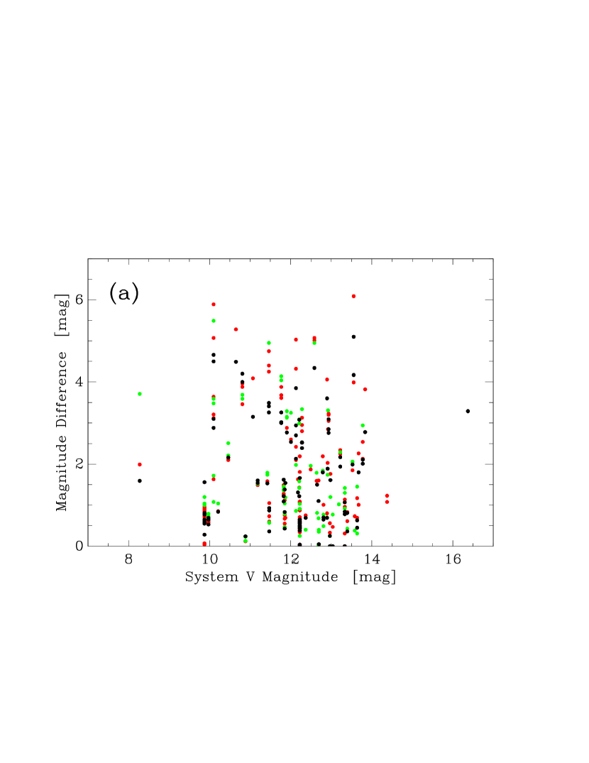
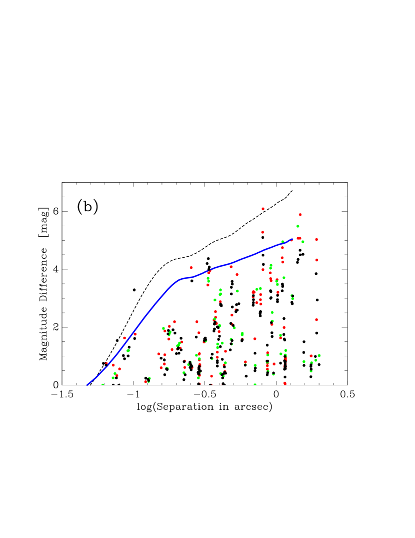
Figure 1: (a) Magnitude difference for all measures listed in Table 1 as a function of the system V magnitude appearing in the literature. (b) The same values plotted versus the log of the separation appearing in Table 1. The dashed curve is the detection limit curve for DSSI at the WIYN at 692 nm, taken from Horch et al. (2017), which as discussed in the text, may not represent the data here as well due to the faintness of these stars. The blue curve is the result of averaging the standard curve with that of a fainter source, which appears to represent the detection limits here better on average. In both plots, the color of the plot symbol indicates the wavelength of the observation: green is used for 562 nm, red is used for 692 nm, and black is used for both 832 and 880 nm.

4 Astrometric Precision

Since our principal aim is to establish if the companions in Table 1 are likely to be gravitationally bound to their primary stars, it is important to characterize the precision of the astrometry we obtain. This in turn is dependent on the derivation of the pixel scale and detector orientation relative to celestial coordinates. For data taken at WIYN with DSSI, a well-established regimen of scale calibration was in place for the entire tenure of the instrument at that site. It was based on the use of a slit mask mounted to the telescope’s tertiary mirror baffle support structure, in the converging beam of the telescope. The distance between slits was well-measured, as was the distance from the mountings surface to the telescope focal plane. When observing a very bright unresolved star with the mask in place, a series of fringes of different spacings is produced in the image of the star on the detector. The effective wavelength of the observation was determined using a spectrum of a star with the same type chosen from the spectral library of Pickles (1998) and combining that flux curve with the known transmission curve of the filter used and the quantum efficiency curve of the detector. In combination with the distance measures mentioned just above and the focal length of the telescope, the fringe spacing can then be determined in arc seconds. By measuring the number of pixels across the fringe pattern, the scale in arc seconds per pixel is obtained. However, the actual measurement is done in the Fourier domain, where the fringes map to sharp line-like features at particular spatial frequencies. A least-squares fit is then performed between the data and a model function representing the pattern of lines where the scale value is the fitted parameter.

The orientation of the detector relative to celestial coordinates was obtained by recording a set of offset images of bright stars, generally once per night. An initial image is taken, and then small offsets in position in different cardinal directions are made with the telescope. The images are reduced and the position of the star in each image is determined via centroiding. This yields the offset angle the orientation of the detector pixels and the cardinal directions north and east on the sky. It also yields an estimate of the scale, but it is generally lower precision than the measures obtained from the slit mask. In some runs, if offset sequences were judged to be of lower quality (for example, if the images were taken in windy conditions or in poor seeing), then the measured orientation angle is supplemented with the value inferred from a small number of binaries observed for the purpose of monitoring scale and orientation over time and referred to as “scale” binaries; these systems generally have extremely high-precision orbits determined from long-baseline optical interferometry (LBOI).

At the LDT and at Gemini, no slit mask was available, so a regimen of observing scale binaries from LBOI was employed, and both scale and orientation were derived solely from those measures. With NESSI observations at WIYN, the slit mask was of course available, but to avoid removing and reinstalling the tertiary mirror baffle for each speckle observing run, the mask was instead mounted to the baffle itself. Since that change, the slit mask scale determinations have been less consistent from run to run compared with the DSSI scale values, and so for the work presented here, we fell back to the same regimen of “scale” binaries as used at the LDT and Gemini when reducing NESSI data. Overall, despite these differences in approach, the scale values appear to be accurate to $\sim$0.2% or better, and the orientation angles to $\sim$0.3^∘, when judged against binaries with well-determined orbits (that were not used in scale determinations).

While obtaining high-precision astrometric calibrations over a period of years at different telescopes is challenging, the effort that we have made to maximizing the long-term astrometric performance provides the basis for the current study. As discussed more fully in e.g. Horch et al. (2011) (for WIYN data), Horch et al. (2012) (for Gemini-N), and Horch et al. (2014) (for the LDT), the astrometric results during the period of observations presented here generally have 1-$\sigma$ uncertainties of between 1 and 3 mas in position in all cases for the standard program of binary star survey observations.

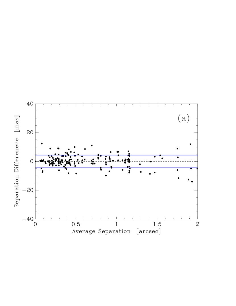
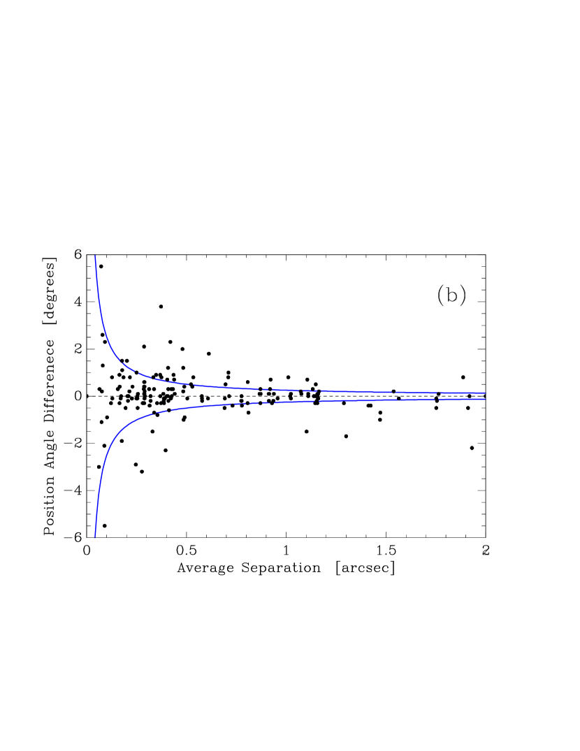
Figure 2: (a) Difference in the separation as a function of average separation for the paired measures in Table 1. The zero line is drawn to guide the eye, and the blue dashed lines represent $\pm 4.4$ mas, the standard deviation of these values. (b) Differences in position angle as a function of average separation. Again, the zero line is drawn, and in this case the blue dashed curves represent the $\pm$1-$\sigma$ uncertainty implied by a linear uncertainty of 4.4 mas.

A unique capability of the DSSI and NESSI instruments is their ability to record two speckle patterns in two filters simultaneously. For astrometric studies, this provides a natural way to characterize the internal astrometric precision of a data set, simply by comparing results obtained independently from the two channels of the instrument, which should yield the same result. In Figure 2(a), we show the separation differences as a function of average separation when subtracting the result in one channel versus the other for all the paired observations appearing in Table 1. Figure 2(b) shows a similar plot for position angle residuals. Separation residuals have an average value of $0.26\pm 0.32$ mas, with a standard deviation of $4.38\pm 0.23$ mas. There are no obvious trends in the plot, except perhaps a slight increase in the scatter at the largest separations. It is in this region of the plot that any systematic errors in the determination of the scale will be seen in addition to the random scatter of the measures; if the scale is slightly overestimated for some runs and slightly underestimated for others, this could lead to a broadening of the residual distribution that is most noticeable at the largest separations. However, there are few data points in this region of the plot which at worst have a modest increase in the scatter, and so we conclude that this is at most a small contribution to the astrometric uncertainty of the data set overall.

In to Figure 2(b), the average value obtained is again close to zero, $0.05\pm 0.08^{\circ}$, and the position angle residuals show the typical increase in standard deviation at small separations. (The average values for the standard deviation throughout the plot is $1.03\pm 0.05^{\circ}$.) This increase is a geometrical effect; if the astrometric uncertainty is equal and independent in the direction orthogonal to the separation, then the position angle uncertainty (in radians) is given by

$$\delta\theta=\frac{\delta\rho}{\rho},$$ (1)

where $\delta\theta$ and $\delta\rho$ are the uncertainties in position angle and separation respectively $\rho$ is the separation of the pair. In Figure 2, we have placed curves on the plot using $\delta\rho=\pm 4.4$ mas, and we see that, in the mean, this appears to provide a reasonable 1-$\sigma$ envelope to the data at all separations. A few measurements have relatively large differences in position angle at large separations, but many of these are extremely faint companions, and harder to fit on that basis.

The differences plotted in Figure 2 are the subtraction of two independent measurements with presumably the same uncertainty, in which case the subtraction has an uncertainty that is $\sqrt{2}$ larger than the uncertainty of either individual measure. This means that the uncertainty in a single measure in Table 1 is given by $4.38\pm 0.23$ divided by $\sqrt{2}$, or in other words, $3.10\pm 0.16$ mas. This is larger than the measurement uncertainty derived in e.g. Horch et al. (2017) for DSSI at WIYN; in that paper the value stated was $1.73\pm 0.04$ mas. The main difference between that data set and the one in Table 1 is the magnitude range of the target stars: in Horch et al. (2017), the stars were mainly in the range $6<V<10$, whereas for the current sample it is $10<V<14$. Therefore the deterioration in the astrometric precision is most likely due to lower signal-to-noise ratios for the stars in this study. Given the consistency between the separation and position angle differences, we will assume moving forward that the linear measurement precision of single measures in Table 1 is 3.1 mas. Likewise, we assume that the average uncertainty in position angle for measures in Table 1 is $1.03^{\circ}/\sqrt{2}=0.7^{\circ}$.

5 Relative Proper Motion Determination of the Secondary with Respect to the Primary Star

Table 2: Proper Motions for KOIs Observed in at Least Three Epochs

KOI	Kepler No.	Speckle $\Delta\mu_{\alpha}$	Speckle $\Delta\mu_{\delta}$	System $\mu_{\alpha}$	System $\mu_{\delta}$	$\pi$	Source
No.	or Disp.	(mas/yr)	(mas/yr)	(mas/yr)	(mas/yr)	(mas)	for $\mu$, $\pi$
1	1	$0.852\pm 1.124$	$-0.417\pm 1.540$	$5.219\pm 0.043$	$1.619\pm 0.043$	$4.615\pm 0.022$	DR2
13	13	$1.042\pm 0.545$	$0.272\pm 0.554$	$-4.401\pm 0.187$	$-15.780\pm 0.237$	$1.905\pm 0.105$	DR2
98	14	$-0.793\pm 0.328$	$0.277\pm 0.237$	$1.0\pm 1.3$	$-10.2\pm 1.0$	$1.449\pm 0.113$	UCAC4, CFOP
118	467	$-16.526\pm 0.932$	$-42.943\pm 0.645$	$14.227\pm 0.038$	$35.604\pm 0.041$	$2.116\pm 0.023$	DR2
120	(PC)	$-6.503\pm 8.617$	$-5.921\pm 5.629$	$-6.9474\pm 0.094$	$-12.249\pm 0.097$	$1.240\pm 0.044$	DR2
177	(PC)	$0.716\pm 0.118$	$0.238\pm 0.161$	$5.5\pm 3.5$	$6.1\pm 1.4$	$2.160\pm 0.155$	UCAC4, CFOP
258AB	(FP)	$1.089\pm 1.118$	$1.012\pm 0.675$	$4.183\pm 0.052$	$-7.309\pm 0.055$	$2.648\pm 0.031$	DR2
258AC	(FP)	$-15.745\pm 1.597$	$-4.521\pm 3.283$	$4.183\pm 0.052$	$-7.309\pm 0.055$	$2.648\pm 0.031$	DR2

Note. — Table 2 is published in its entirety in the machine-readable format. A portion is shown here for guidance regarding its form and content.

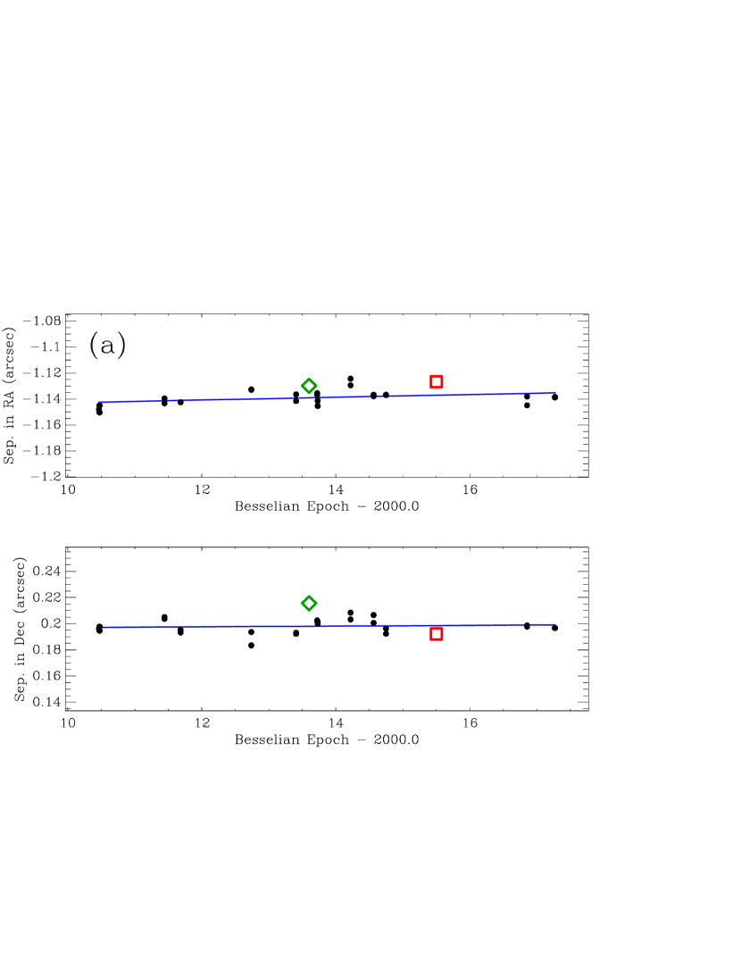
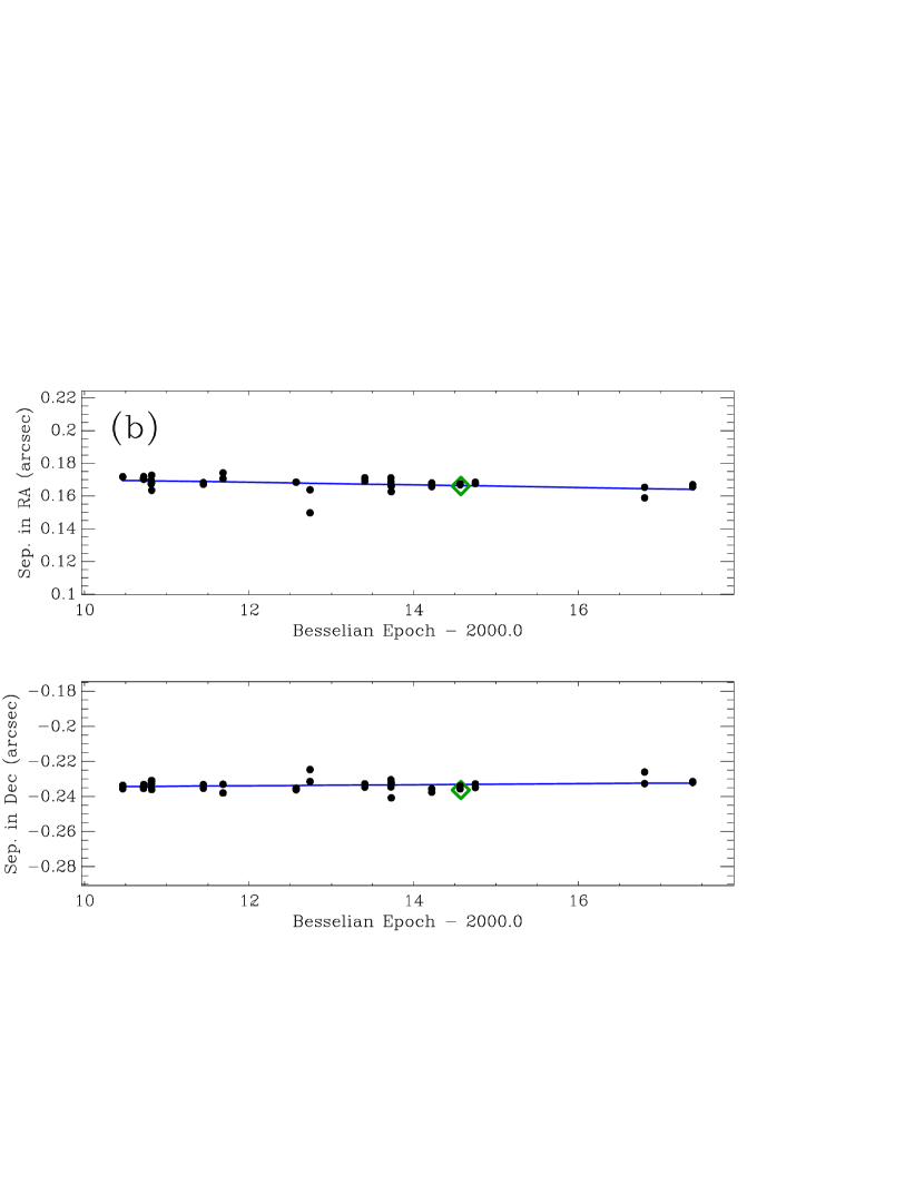
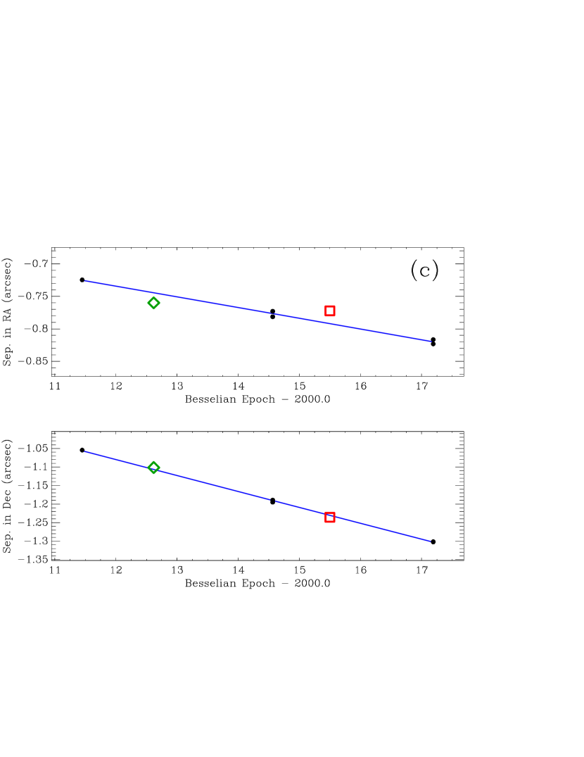
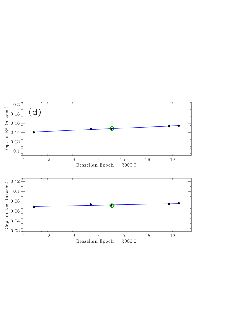
Figure 3: Plots of the projected separation as a function of time for four representative stars in Table 2. Filled circles represent data points from Table 1, the red open squares mark the Gaia DR2 measurement (at J2015.5) if available, and the green diamonds are measures from Kraus et al. (2016). The linear fit for each system, obtained as described in the text, is shown in blue, yielding the relative proper motion values appearing in Table 2. (The fits do not include the Gaia or Kraus et al. measures.) (a) KOI 13 = Kepler-13. (b) KOI 98 = Kepler-14. These two systems illustrate our results on extremely well-observed pairs. (c) KOI 118 = Kepler 467. (d) KOI 270 = Kepler 449. These latter two examples show systems with the minimum or near-minimum number of observations to be included in Table 2.

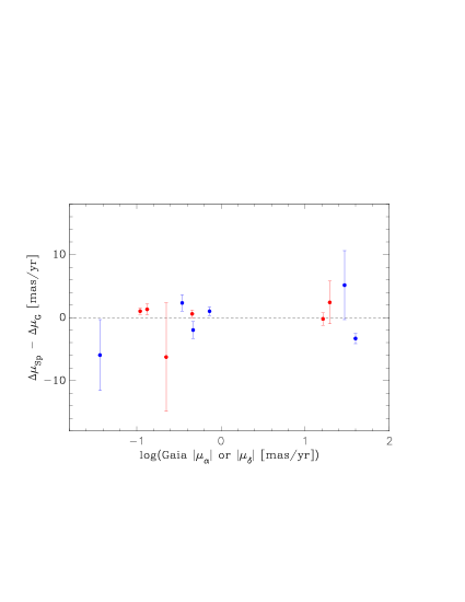
Figure 4: A comparison of the relative proper motions derived from the speckle data set versus those in the Gaia DR2 for the six systems in Table 2 for which Gaia values exist. The ordinate is the (speckle minus Gaia) difference in $\Delta\mu_{\alpha}$, shown in red, and in $\Delta\mu_{\delta}$, shown in blue.

Given that most objects in Table 1 have observations at three or more epochs, we can use the positional information over time to the determine relative proper motion of the secondary with respect to the primary. For this purpose, we compute the separation projected onto the right ascension and declination system at each epoch. We perform a linear least-squares fit to the separation in each coordinate as a function of time, where all data points receive equal weight. From this, we can derive the slope of the line and its uncertainty, which represents the relative proper motion, $\Delta\mu_{\alpha}$ for right ascension, and $\Delta\mu_{\delta}$ for declination. Table 2 gives results for $\Delta\mu_{\alpha}$ and $\Delta\mu_{\delta}$ for all objects in Table 1 that were observed at three or more different epochs, and Figure 3 shows the fits obtained in four representative cases. We also plot there the positions from the Gaia DR2 (Gaia Collaboration, 2018) in two cases, and from Kraus et al. (2016) in all four cases. We have compared the linear fits with and without the Kraus et al. data, for example, but see little difference in the uncertainties of the derived proper motions. To guard against introducing any systematic offsets in position from different studies, we include only our own measures in deriving the proper motions. Also in Table 2, we show the proper motion of the primary star (if resolved) or the system (if unresolved) as it appears in the literature, generally either from the Gaia DR2, Tycho-2 (Høg et al., 2000), or UCAC4 catalogs (Zacharias et al., 2013). We also include the best known parallax, $\pi$, for the object from the literature.

With regard to the DR2 proper motions and parallaxes, the sample represents a range of uncertainty values in these quantities, with the least precise values comparable to the ground-based sources we have used when DR2 values are not available. We examined the Renormalized Unit Weight Error (RUWE) values for those objects in our sample, and as expected, a majority of our stars have a high value of this quantity, which can indicate unresolved binaries and other problems with the astrometric solution. Nonetheless, the RUWE values scale roughly linearly with uncertainties in proper motion and parallax for our stars, and so we find no evidence to suggest that the DR2 values are not reliable to the level that their uncertainties indicate.

There are six cases from Table 2 where both components are measured separately in DR2, all of which have separations larger than one arc second (due to the resolution limitations of DR2). In Figure 4, we compare our relative proper motion for the secondary versus what can be derived from the proper motion of both components from DR2. We find no systematic offset in either $\Delta\mu_{\alpha}$ or $\Delta\mu_{\delta}$, giving confidence that the methodology used on the speckle data is sound.

6 Analysis of the Motions

We investigate the motions derived in the previous section in two ways. First, one can compare the relative motion of the components in our sample with what would be expected for line-of-sight (LOS) companions. In this case if the motion we observe is small compared to the mean motion of optical doubles, then the pair may be considered to be co-moving, or in other words, a common proper motion (CPM) pair, and thus likely to be physically associated. On the other hand, we can also study the motions we observe in comparison to the expected motions of orbiting companions with similar distances and masses. If the relative proper motion is consistent with the typical motion one would observe from a bound companion, then that can be used as further evidence of the nature of the system. While neither approach is definitive in terms of characterizing the companions as bound or unbound, both together can give a strong indication of the physical proximity of the two stars.

6.1 Common Proper Motion

The stars in our sample cover a substantial distance range, from roughly 100 to 1800 pc, and the average proper motion will decrease as the distance grows. Therefore, we form the ratio of the magnitude of the relative proper motion vector we derive to the magnitude of the system proper motion vector. We will refer to this ratio as $R_{1}$, so that

$$R_{1}=\frac{|\Delta\vec{\mu}|}{|\vec{\mu}_{1}|},$$ (2)

where $|\Delta\vec{\mu}|$ is the magnitude of the relative proper motion vector and $|\vec{\mu}_{1}|$ is the magnitude of the system proper motion vector, or that of the primary star if available. If the pair exhibits CPM, then $R_{1}$ should be near zero, while if the companion is a distant background star, then the ratio will be near unity, since the background star’s proper motion in general will be much smaller than that of the primary star. Alternatively, if the companion is a dim foreground star, the ratio is more likely to exceed unity, since in that case the relative proper motion will be dominated by the motion of the secondary star. A pair of unknown disposition can be judged as likely to be a CPM pair if its ratio is small, and more likely to be an optical double if the ratio is near one or above.

To understand the expected properties of this ratio for our sample, we chose two samples of 2000 stars from the Gaia DR2 catalogue near the center of the Kepler field. The first sample was selected to have $G$ magnitudes between 10 and 14 and parallaxes greater than 0.555 mas, the smallest parallax in our sample of KOIs. The second sample had $G$ magnitudes between 10 and 18 with no parallax restriction. A small number of stars were common to both samples, and these were removed from consideration, leaving two independent samples of 1944 stars each. We then form a hypothetical optical double by randomly pairing a star from the first sample to act as a primary star and a star from the second sample to act as a secondary. The DR2 data was used to compute the relative proper motion between the stars, and we form the ratio $|\Delta\vec{\mu}|/|\vec{\mu}_{1}|$ using the primary’s proper motion. We select from the sample only systems with magnitude differences between 0 and 4.6 (roughly matching our expected detection limit) for inclusion in the final sample. This left a total of 1366 optical pairs, from which we can study the statistics. The ratio $R_{1}$ is plotted as a function of distance for the final sample in Figure 5(a). As expected, the sample has a median value near 1, indicating that in most cases the companion is a background star that moves little in comparison to the closer primary star; hence, the relative proper motion is nearly the same value as $|\vec{\mu}_{1}|$.

Foreground companions (which by construction are always dimmer than the primary) represent 11.7% of the cases in the final sample overall and have a higher median value, near 1.6. Indeed, if only stars above the median line in the plot are considered, foreground companions then represent 15.5% of the sample. 45.6% of companions above the 95% line are foreground stars.

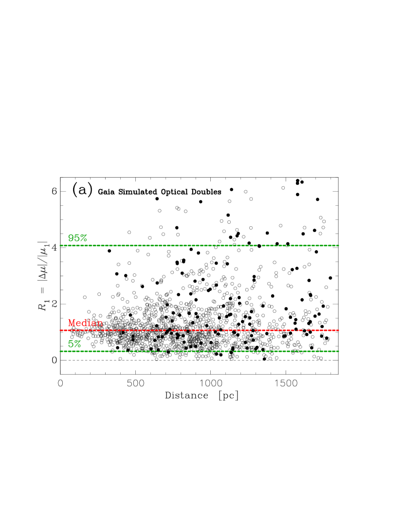
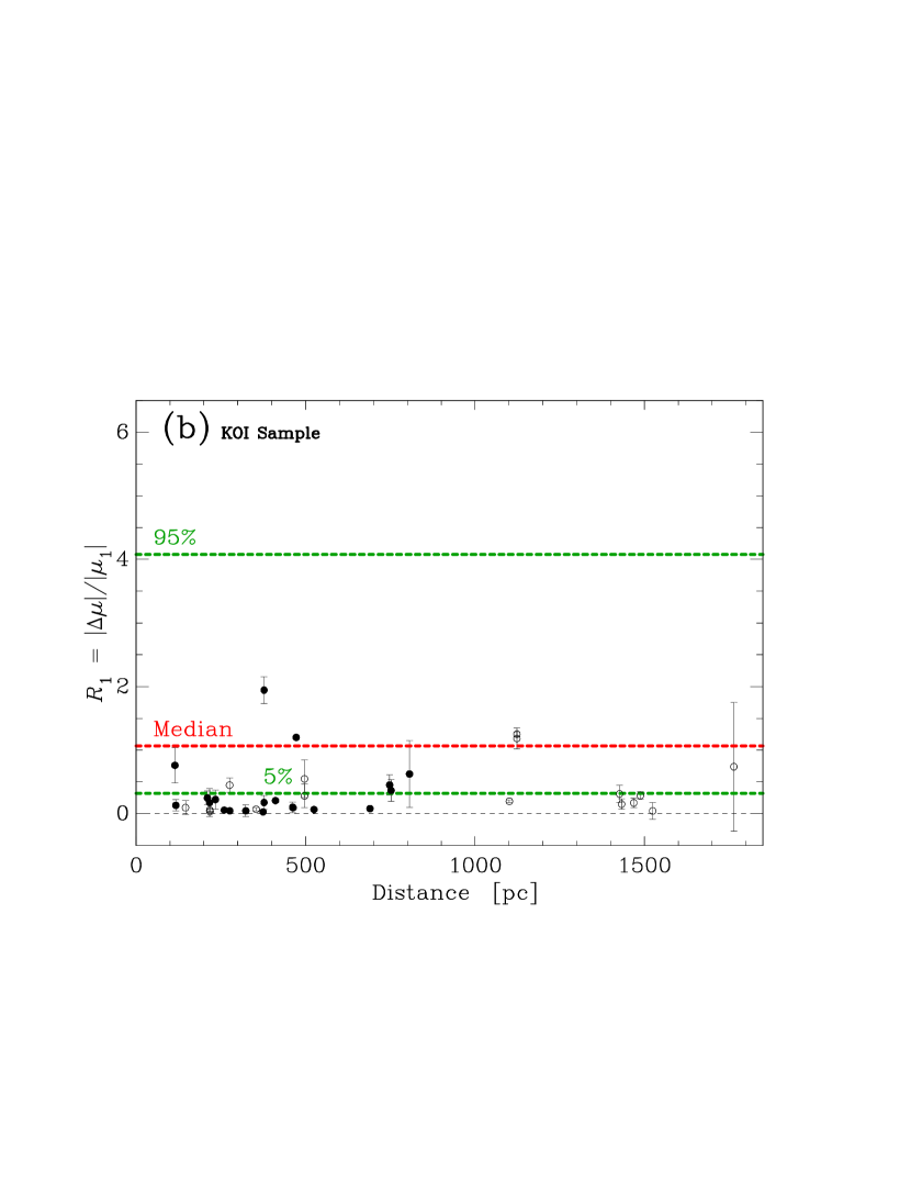
Figure 5: The ratio $R_{1}$ (the magnitude of the difference in proper motion between primary and secondary divided by the proper motion of the primary) as a function of distance. (a) In this panel, we show stars from the Gaia DR2 catalog located near the center of the Kepler field that have been selected and randomly paired with a second star to approximately match the magnitude differences of the stars in Table 2. The primary stars have distances in the range of 0 to 1800 pc and Gaia $G$ magnitudes between 10 and 14. This simulates a population of line-of-sight companions as discussed in the text. Foreground companions are shown as filled circles, and background companions as open circles. (b) Here, we plot the same for the stars in Table 2, where filled circles indicate systems with parallax measures with uncertainties under 10%. In both panels, the dashed lines indicate the percentage of stars in (a) that have a ratio below the line drawn, thus the lower green line is the 5% contamination line of optical doubles.

The results in the plot also show that only 5% of hypothetical optical doubles have $R_{1}<0.32$ over the distance range of our sample. In Figure 5(b), we show the same plot for the KOI sample. The majority of stars have ratios below 0.32, and thus may be viewed as likely to be common proper motion pairs. We also find three of our systems (including one triple, KOI 1792) above the median line; these are almost certainly not CPM pairs. KOI 1792 will be discussed further in Section 7.

Although the majority of our systems appear likely to be CPM pairs, it is wise to remain cautious at this stage concerning a determination. Figure 5(a) illustrates that, although unlikely, chance similarities in proper motions can exist that will make a physically unbound system appear to be a CPM pair, particularly for distances larger than 300 pc, which is a large majority of our sample.

6.2 Orbital Motion

For the stars in our sample, we do not expect large changes in the relative position of the components due to orbital motion over the time that we have observed them, given the range of distances represented and the likelihood of very long periods, if bound. Nonetheless, as a simple example, a 2$M_{\odot}$ system with a semi-major axis of 500 AU in a face-on circular orbit at a distance of 1 kpc will have a period of 7900 years and an observed separation of 0.5 arcsec, and therefore move about 0.4 mas/year on the sky, a number that is comparable to many of the uncertainties stated for the relative proper motions in Table 2. For that reason it can be expected that in at least some cases, the orbital motion will be above the measurement precision represented by our data set.

To investigate this, we define the quantity $R_{2}$ as follows:

$$R_{2}=\frac{|\Delta\vec{\mu}|}{|\Delta\vec{\mu}({\rm avg,orb})|},$$ (3)

where $|\Delta\vec{\mu}|$ is again the magnitude of the relative proper motion vector between the primary and secondary star, and the quantity $|\Delta\vec{\mu}(\rm avg,orb)|$ is an estimate of the expected average change in relative position per year assuming that the system is gravitationally bound. As with the previously defined quantity $R_{1}$, creating a ratio has the virtue of removing the decrease in the observed angular motion with increasing distance. We can also anticipate that if the denominator is estimated well, then the average value of $R_{2}$ for bound companions will be near 1. If the system is a line-of-sight companion, then $R_{2}$ can scatter toward values that are significantly larger than 1 in general since in that case the proper motion of either star can be a few to 10’s of mas per year (as shown in Table 2). This is much larger than the typical orbital motions, and the numerator of $R_{2}$ will therefore be much larger than the denominator.

We estimate the quantity $|\Delta\vec{\mu}({\rm avg,orb})|$ by starting with the effective temperatures for the KOIs in Table 2 as they appear in the Exoplanet Follow-up Observing Program (ExoFOP) website for Kepler. In many cases there are estimates made by multiple observers, and in those cases the average values were calculated, together with the standard errors. Individual effective temperature measures often have uncertainty estimates, and in general we find that these are consistent with the values derived by computation of the standard error. On average, the errors we obtain in the temperatures in this way are roughly 100K.

Next, the temperatures are used to estimate the mass, spectral type, and absolute $V$ magnitude of the primary star. A standard reference, Schmidt-Kaler (1982), is used for that purpose. We then take the average magnitude difference for each KOI in Table 2 in the 562-nm filter and we use that to estimate the absolute $V$ magnitude of the secondary star, on the assumption that it is at the same distance as the primary star (i.e. that the system is bound). Schmidt-Kaler (1982) is then used to arrive at the mass of the secondary star and a total mass estimate for the system is computed. Two stars in our sample, KOI 258 and KOI 977, are listed as giants in SIMBAD   (Wenger et al., 2000); this was taken into account in computing the masses, but otherwise primary stars are assumed to be dwarfs.

Finally, using the observed separation as a proxy for the semi-major axis of the orbit, we compute a period estimate $P$ according to Kepler’s harmonic law:

$$P=\sqrt{\frac{\rho^{3}}{\pi^{3}M_{\rm tot}}},$$ (4)

where $\rho$ is the separation of the pair, $\pi$ is the parallax, and $M_{\rm tot}$ is the estimated total mass of the system. The estimate of $|\Delta\vec{\mu}({\rm avg,orb})|$ is then obtained by computing the total distance traveled in one orbit on the plane of the sky, that is, computing the perimeter of the observed orbital ellipse, and dividing that by the period itself. This gives an average distance covered per year, or equivalently, an average value for the observed relative proper motion due to orbital motion. The perimeter of the ellipse will vary with the various orbital elements, in particular the inclination $i$, the eccentricity $e$, and the ascending node $\Omega$, which of course are not known. However, the perimeter should scale with the semi-major axis and be dependent on orbital geometry; for an edge-on circular orbit of semi-major axis $a$, the total distance on the sky that is traveled in one orbit is $4a$. On the other hand, for a face-on circular orbit, the result is $2\pi a$. Thus, we can infer that for any other orbit, the total length of the orbit in the plane of the sky is a geometrical factor times the semi-major axis, and that the factor is of order 5. Using the initial mass function found in Kroupa (2001), we constructed a simulation of 5000 primary stars and then chose binary companions and orbital parameters using Raghavan et al. (2010). The length of the perimeter of each orbit in the plane of the sky was then calculated, and compared to the semi-major axis. This exercise showed that, on average, the value of the geometrical factor is approximately 4.6. Therefore we propose to calculate $R_{2}$ from observational data using the following method:

$$R_{2}=\frac{|\Delta\vec{\mu}|}{|\Delta\vec{\mu}({\rm avg,orb})|}=\frac{|\Delta\vec{\mu}|\cdot P}{4.6\cdot\rho}=\frac{|\Delta\vec{\mu}|}{4.6}\sqrt{\frac{\rho}{\pi^{3}M_{\rm tot}}}$$ (5)

We used a sample of simulated binaries to inform us how our proposed quantity $R_{2}$ behaves for the KOIs in Table 2. Again employing our simulation of 5000 orbits, and we assign distances with a Gaussian distribution with the same mean and standard deviation as the sample of stars in Table 2. We check to make sure that the apparent magnitude, separation, and magnitude difference of each system falls in the range that we could observe with DSSI. Finally, we compute a value of $|\Delta\vec{\mu}|$ at a random point in the orbit, and form $R_{2}$ as shown in Equation 5. The results are shown in Figure 6(a) and they indicate that these simulated binaries have $R_{2}$ values that cluster around 1 regardless of distance, and that only 5% of the orbits generate an $R_{2}$ value greater than 1.87. Computing the value of $R_{2}$ for our data, we obtain the plot in Figure 6(b). In this case we see that the majority of our stars have motions that are consistent with orbital motion, but that some do have values much higher than 1.87, which indicates that the relative motion cannot be explained by mutual gravitational attraction, at least given the mass estimates used. We investigated how sensitive the ratio is to the mass sum of the simulated binaries and found that if masses twice as large were used in generating the orbits used in the simulation, the 95% line drawn in Figure 6 would increase to 1.80 (the log of which is 0.26). Given the range of $R_{2}$ values of the KOI stars we have studied, this is not a large change. Thus we conclude that our results are not strongly dependent on the mass estimates we have made.

Kervella et al. (2019) use a similar methodology to determine the physical association of galactic Cepheids and RR Lyrae stars in Gaia DR2; however, in their case they use the total mass and separation to compute an estimate of the escape velocity of the system. This is then compared with the relative proper motion. We note that the denominator in Equation 5 has the same dependence on total mass and separation as the standard escape velocity formula, namely

$$v_{\rm esc}=\sqrt{\frac{2GM_{\rm tot}}{r}}\sim\sqrt{\frac{M_{\rm tot}}{r}},$$ (6)

and therefore our method is based on essentially the same physics, and at most differs in the exact value of $R_{2}$ that is used to differentiate between bound and unbound companions; however, our method has more detail in the sense that known statistics of the orbital parameters of field binaries are incorporated into the model.

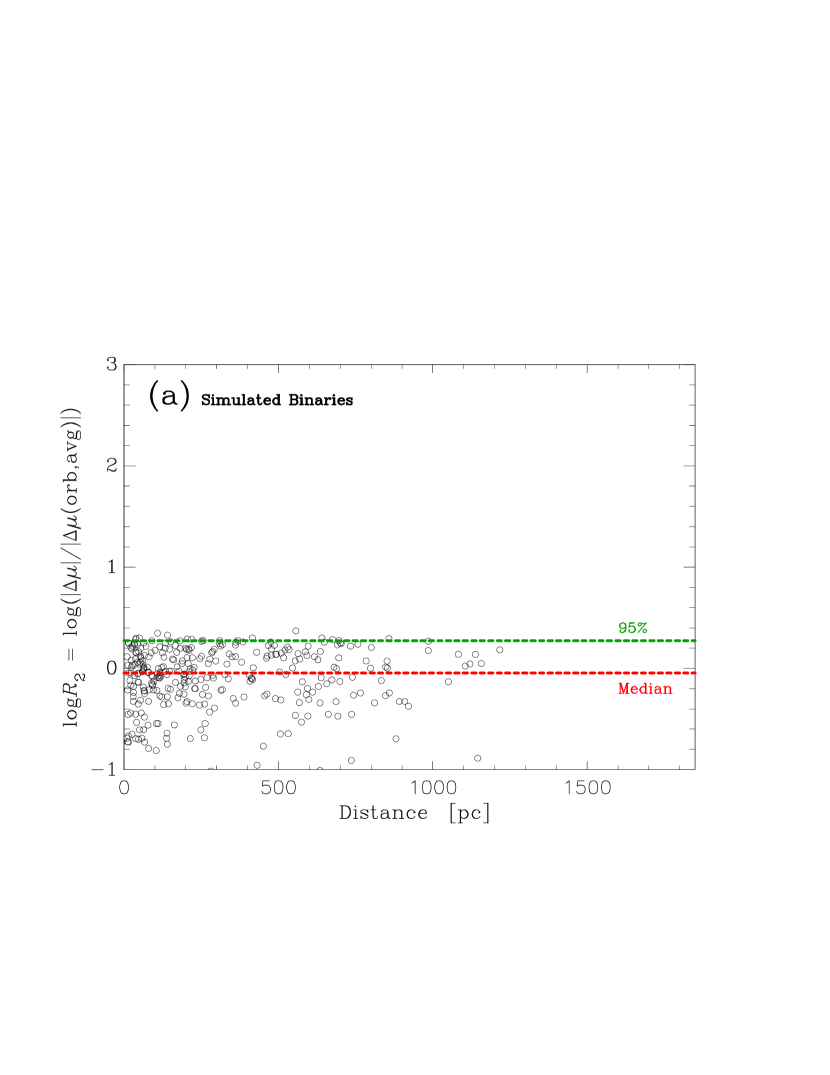
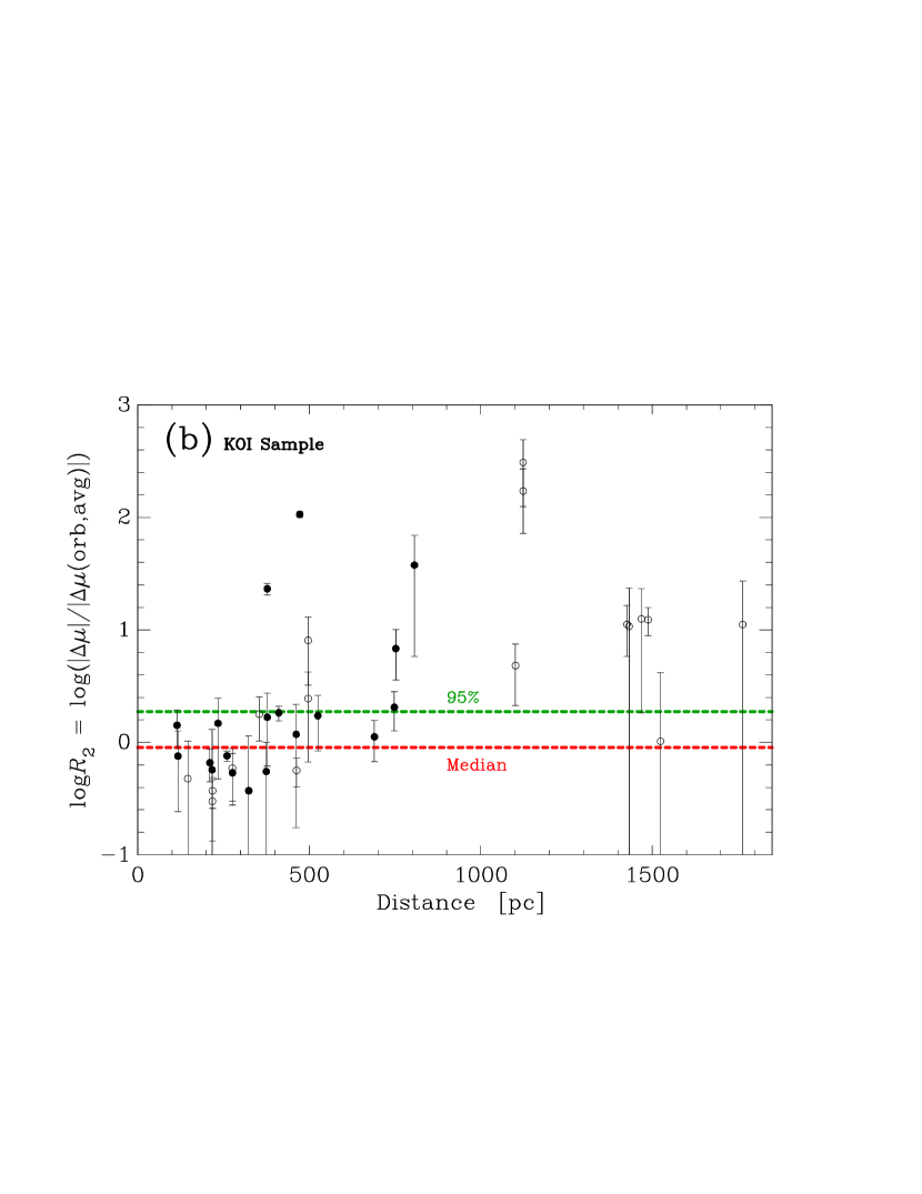
Figure 6: The log of the ratio $R_{2}$ (the magnitude of the difference in proper motion between primary and secondary divided by the derived estimate of the average relative proper motion based on the assumption of orbital motion), plotted as a function of distance. (a) In this panel, we show the simulated distribution created as described in the text for bound companions. (b) Here, we plot the same for the stars in Table 2. In both panels, the dashed lines indicate the percentage of stars in (a) that have a ratio below the line drawn.

7 Properties of the Sample

Table 3 contains the final information for our 34 well-measured systems, showing columns for (1) KOI number; (2) Kepler number if any; (3) the number of confirmed exoplanets in the system, (4) the distance to the system; (5) the estimate for the primary mass; (6) the estimate for the secondary mass; (7 and 8) the values for $R_{1}$ and $R_{2}$ obtained from the analysis in the previous section; and (9) final comments regarding the disposition of each system. If a Gaia DR2 parallax is available, the distance value in Column 5 is that in Bailer-Jones et al. (2018) rather than simply inverting the Gaia DR2 parallaxes. The differences in all cases except KOI 1890 are small, generally within a few percent, with no systematic trend for our small sample.

From this, we can conclude that the majority of these systems are highly likely to be gravitationally bound, and that a few are obvious LOS companions. The final disposition for each system, shown in the rightmost column, is determined from $R_{1}$ and $R_{2}$ as follows:

$\bullet$ A system is judged to be a CPM pair if $R_{1}+\delta R_{1}<0.32$ and $R_{2}-\delta R_{2}<1.87$. This occurs when (1) the full uncertainty interval for $R_{1}$ falls below the 5% line in Figure 5(b) so that we can confidently claim that the pair is co-moving and the (2) uncertainty interval for $R_{2}$ overlaps with the 95% probability line in Figure 6(b), indicating that the motion is consistent with at least some fraction of orbital possibilities for the system.

Table 3: Final Properties of 37 KOI Double Star Components

KOI	Kepl. No.	No. of	Distance	$M_{1}$	$M_{2}$	$R_{1}$	$R_{2}$	Comments
No.	or Disp.	Planets	(pc)	($M_{\odot}$)	($M_{\odot}$)
1	1	1	$215.3^{+1.1}_{-1.0}$	0.97	0.51	$0.174\pm 0.223$	$0.57\pm 0.73$	CPM?
13	13	1	$519.1^{+30.7}_{-27.5}$	1.60	1.48	$0.066\pm 0.033$	$1.73\pm 0.89$	CPM
98	14	1	$690.1\pm 55.7$	1.40	1.12	$0.082\pm 0.032$	$1.12\pm 0.45$	CPM
118	467	1	$466.3^{+5.1}_{-5.0}$	0.89	(0.46)	$1.200\pm 0.018$	$106.16\pm 5.99$	LOS
120	PC	…	$789.4^{+28.5}_{-26.6}$	1.12	(1.00)	$0.625\pm 0.527$	$37.60\pm 31.78$	Uncertain

Note. — Table 3 is published in its entirety in the machine-readable format. A portion is shown here for guidance regarding its form and content.

$\bullet$ A system is judged to be a probable CPM pair (labeled “CPM?” in Table 3) if $R_{1}<0.32$ and $R_{2}-\delta R_{2}<1.87$, and it is not already in the previous category. This relaxes the restriction on $R_{1}$ so that the measured value itself has a less than 5% probability of being due to random, unrelated motion, but the uncertainty interval includes higher probabilities.

$\bullet$ A system is considered to be a LOS companion if $R_{1}-\delta R_{1}>0.32$ and $R_{2}-\delta R_{2}>1.87$. In this case, the full uncertainty interval for $R_{1}$ is consistent with random motions between the two stars, and the full interval of $R_{2}$ is too high to be consistent with orbital motion.

$\bullet$ A system is labeled as “uncertain” if it does not fit into one of the above three categories. One other system is also labeled as uncertain, KOI 959; this object has no parallax value in the literature, and therefore we cannot form $R_{2}$ to complete the analysis here. However, judging from the value of $R_{1}$ and its uncertainty, the system is likely to be a CPM pair. The proper motion is large, and the spectral type listed in SIMBAD is M+M. The system may therefore be quite nearby.

The placement of our systems in a $\log R_{2}$ versus $\log R_{1}$ diagram is shown in Figure 7(a). Of the 37 components, 17 are CPM, 4 are probable-CPM, 4 are LOS, and the remaining 12 are of uncertain disposition. Of those systems with confirmed exoplanets, 10 are CPM, 2 are probable-CPM, 2 are LOS, and 4 are uncertain. Neglecting the uncertain systems, these latter statistics show that the fraction of CPM systems for the exoplanet host systems in the sample is 12 of 14, or $85.7\pm 9.4$%, which is consistent with the percentage predicted in Horch et al. (2014), where 96% of systems discovered at WIYN and 84% of those discovered at Gemini were predicted to be gravitationally bound. Looking at the magnitude differences and separations of the three LOS companions, all of these fit into the region where LOS companions are expected to be found in Figures 8 and 9 of Horch et al. (2014). This is shown in Figure 7(b). Five systems with more than one confirmed exoplanet are in our sample: KOI 270, KOI 279, KOI 284, KOI 307, and KOI 1792. Of these, three are CPM systems, 1 is LOS, and 1 is uncertain.

These results may be compared with other studies of KOI double stars already in the literature that make a determination of whether the pair was bound or unbound using other methodologies. Atkinson et al. (2017) and Zielger et al. (2018) both make a judgement using a photometrically-determined distance for both components; if the distance derived for the two stars is consistent within the uncertainty, then they infer that it is highly likely that the pair is physically associated. They both compute a value to assess the probability of being bound based on the differences in the two distances in terms of their estimated uncertainties, the quantity they call “$\sigma_{\rm unbound}$,” with larger values implying a smaller chance that the system is physically associated. In the case of Atkinson et al. (2017), although seven systems are common to both their study and ours, we judge three of these to be uncertain, and so there are only four cases where a clear comparison can be made, namely KOI 984, 1613, 2059, and 5578. Both studies find that the first three are all CPM or CPM? systems, but we find that KOI 5578 is CPM while Atkinson et al. find a $\sigma_{\rm unbound}$ value above 3, higher than what would be expected for a bound system. For Zielger et al. (2018), six systems are common to both studies, one of which we judge to be uncertain. We find clear agreement in three cases (KOI 1, 1792, and 2059), and apparent discrepancies in two others (KOI 13 and 984). Again, we find these are likely bound while Ziegler et al. find $\sigma_{\rm unbound}$ values above 3.

The greatest overlap between our results and previous work is found in Hirsch et al. (2017). Those authors also attempted to determine whether the companions to KOI stars are bound through photometric means, but in their case via H-R diagram placement of the components. If the two stars were consistent with a common isochrone, the pair was judged to be bound. As with Atkinson et al. (2017) and Zielger et al. (2018), a direct comparison cannot be made in every case as either Hirsch et al.’s study or ours obtains an uncertain result, but for the 19 companions where both studies make a determination, there is agreement in 17 cases (15 CPM or CPM? that Hirsch et al. judge as bound, and 2 LOS that Hirsch et al. judge as unbound). In two cases, KOI 270 = Kepler-449 and KOI 984, Hirsch et al. found that the system is unbound, yet our measured motions to date indicate a co-moving pair; in the case of KOI 984, we judge it to be a probable-CPM pair. This system has a large separation, leading to potentially over-estimated magnitude differences in speckle observations due to speckle decorrelation (as noted in the observations in Table 1), and so this might have affected the Hirsch et al. photometric result. For Kepler-449, this is not a concern as this object has a small separation, so it is possible in this case that there is simply a chance alignment in velocities to make the pair appear co-moving. However, looking at the additional differential photometry available in Table 1 and combining that with what Hirsch et al. had available earlier, we note that the preponderance of the evidence points to a pair with modest magnitude difference at all observed wavelengths, which suggests that it would be possible to reconcile the photometry with a common isochrone for both stars, assuming both stars are dwarfs. Four exoplanet host systems from our sample of particular note, including Kepler-449, are discussed below.

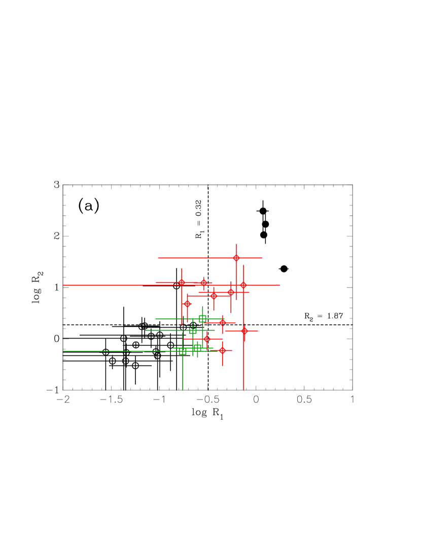
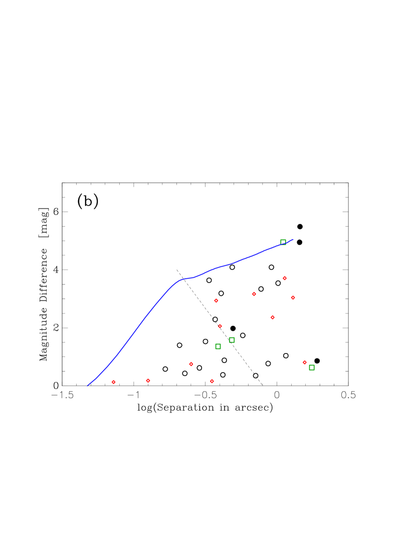
Figure 7: (a) A plot of $\log R_{2}$ as a function of $\log R_{1}$ for the 35 components that have both values listed in Table 3. (b) A plot of magnitude difference as a function of separation for the components in Table 3. In both plots, open circles are CPM pairs, open green squares are the probable-CPM pairs (listed at “CPM?” in Table 3), filled circles are LOS companions, and small red diamonds are the systems of uncertain disposition. In panel (a), the values of $R_{1}$ and $R_{2}$ used to make the final determination for each system are drawn as dashed lines; in general, we expect LOS companions to be in the upper right while CPM pairs are in the lower left. In panel (b), the same detection limit curve as in Figure 1(b) is drawn, and the dashed line indicates the approximate demarcation between the region where LOS companions are not found (below the line), and the region where there is a mix of bound and unbound companions (above the line) in the simulations detailed in Horch et al. (2014).

Kepler-13 (KOI 13). The photometric analysis of Hirsch et al. (2017) showed that the secondary star in this system (which has one confirmed exoplanet) is likely to be a bound companion. The preliminary astrometric analysis of Hess et al. (2018) reached the same conclusion, and with additional data, we also find that the relative proper motions confirm this determination, though as just mentioned, Zielger et al. (2018) reach a different conclusion. This system was also studied in detail by Howell et al. (2019), so assuming its determination as CPM pair is correct, it is one of the few KOI binary systems for which it is known observationally that the exoplanet orbits the primary star and not the secondary.

Kepler-449 (KOI 270). This solar-type star hosts two exoplanets with orbital semi-major axes of 0.1 and 0.2 AU respectively, both of which have current mass estimates below $2M_{\oplus}$. The companion star has a projected separation of 43 AU. If the stellar companion is orbiting in the same plane as the planets (i.e. the inclination of the stellar orbit is near 90^∘), then the minimum period for the stellar orbit (obtained by assuming we are observing the maximum separation at the present time) would be approximately 230 years, given the total mass estimate in Table 3. The motion of this object is shown in Figure 3(d) and further discussed below; despite its relatively small separation and proximity to the Solar system compared with other stars in the sample, we do not see obvious evidence for acceleration in our observations at this point.

Kepler-132 (KOI 284). Similar to KOI 270, this star has effective temperature near that of the Sun, and is a multi-planet system, hosting four known exoplanets. Three have orbital semi-major axes of less than 0.2 AU, but the fourth orbits in a nearly circular orbit of 0.44 AU and period of 110 days. All have current mass estimates below $2M_{\oplus}$. The stellar companion has a large projected separation compared with these planetary orbits, 240 AU, but is less than one magnitude fainter than the primary star. Making the same calculation as above for the orbital period, we find that, if the stellar component is co-planar, it would have an orbital period greater than 3000 years.

Kepler-953 (KOI 1792) This star hosts three confirmed exoplanets, and has $R_{1}>5$ and $R_{2}>100$ for both the B and C components. As can be seen in Table 2, both the B and C components have the same relative proper motion to the primary star, thus these fainter two stars are traveling together and form a CPM double. The large value of both $R_{1}$ and $R_{2}$ points to a slightly elevated probability of the fainter pair being interposed along our line of sight in the direction of the exoplanet system, but on the other hand, the C component is resolved from AB in DR2, and it would appear to have a smaller parallax than AB, indicating that it would be a background pair. Currently, the parallax uncertainty is too large to make a definitive statement from DR2 alone, however.

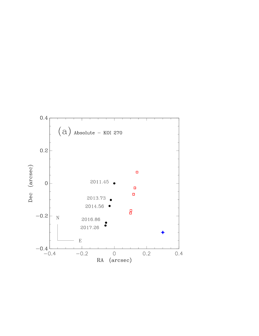
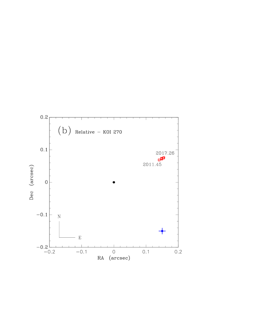
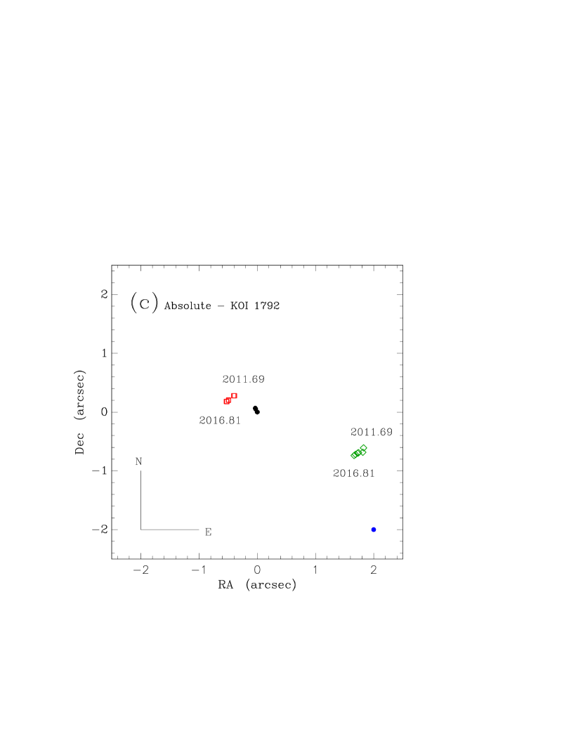
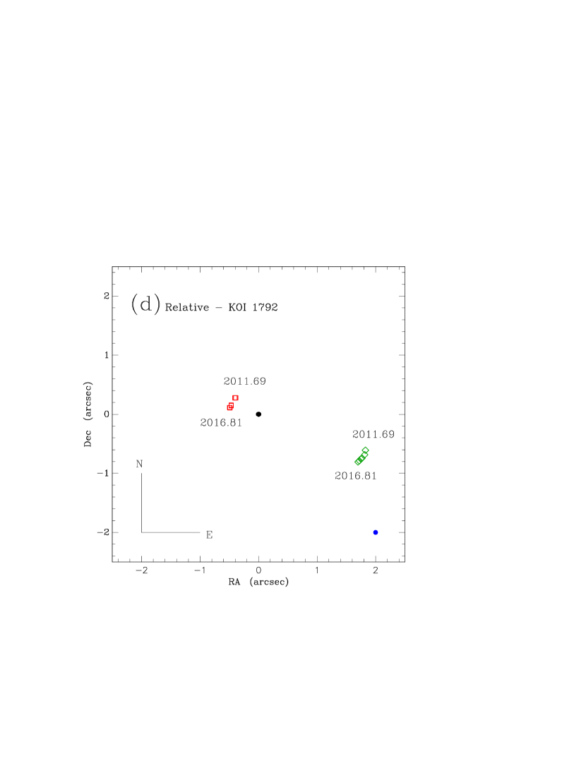
Figure 8: Absolute and relative motions of KOI 270 (Kepler-449, top) and KOI 1792 (Kepler-953, bottom). In all cases, the solid circles represent the location of the primary star, red squares indicate the secondary, and green diamonds represent the tertiary. The blue point in the lower right indicates the uncertainty of the total distance traveled over the period of time shown; it is the uncertainty in the proper motion multiplied by the time baseline. (a) The absolute motions of the two stars in the KOI 270 system ; this is judged to be a common proper motion pair. (b) The relative motion of the secondary star in KOI 270 relative to the primary. The motion seen here is consistent with an edge-on orbit at this point, though the separation is currently increasing and the likelihood of a long orbit is high if the system is bound. (c) The absolute motions of the triple star KOI 1792. (d) The relative motions of the secondary and tertiary stars with respect to the primary for KOI 1792. Here we see that the fainter pair is moving together, in a direction nearly orthogonal to the system proper motion.

In Figure 8, we show a further visualization of the motions of KOI 270 (Kepler-449) and KOI 1792 (Kepler-953). In panel (a) we show the motion on the sky for KOI 270, as derived from the system proper motion and the relative positions over time. In panel (b) the motion of the secondary star relative to the primary is plotted. Panels (c) and (d) show the same two plots for KOI 1792. In the case of KOI 270, the system has a relatively large proper motion, which clearly dominates over the relative motion. Nonetheless, when the relative motion is plotted, the motion of the secondary is clearly revealed to be in a direction radially away from the primary. In the case of the triple star KOI 1792, we see that the secondary and tertiary stars are on opposite sides of the primary, yet they move together in a direction nearly orthogonal to the (small) proper motion of the system as a whole. Thus, the second and third components form a co-moving pair that is not related to the central star.

8 Discussion

With a future analysis carried out over a longer time baseline, it may be possible to see orbital motion develop in some systems studied here. Regular observations of these systems would have to be done over at least the next decade and a rigorous astrometric calibration regimen would need to be maintained, but for the fastest moving cases, such a program may yield evidence of deviations from linear relative motion. The motions detected so far on our sample of stars do not show convincing evidence of orbital acceleration, but this is not surprising given projected separations, which are generally in the range of 100s of AU. Nonetheless, we did attempt to find and examine the most likely cases where orbital motion may reveal itself in the coming years. To do this, we consider the region of Figure 7 in the lower left part of the plot, where the projected separations are the smallest and the masses of the components will be comparable. Cross-referencing those systems with their distances and selecting those with the smallest distances (so that the angular separation represents a smaller physical separation), we find that two systems that are most worthy of future study in this regard are KOI 270 (Kepler-449) and KOI 1613 (Kepler-907), both of which have current projected physical separations between 40 and 50 AU. In the former case, as already discussed, the motion observed so far is in a direction along the separation vector, as would be expected in the case of an edge-on system, implying that this stellar companion’s orbit is possibly co-planar with the orbit of the planet in that system. In the latter, the uncertainties in the relative proper motions preclude a definitive statement on the direction of the secondary’s motion relative to the primary at this stage. However, the values measured here suggest that it is not obviously consistent with an edge-on orbit, and if that were to be the case, it would represent an orbit that cannot be co-planar with the planet in that system. At least several more years of data will be needed to determine if these hypotheses are correct. Two other systems with confirmed exoplanets, KOI 307 (Kepler-520) and KOI 2059 (Kepler-1076), have current projected separations in the range of 50-100 AU, and will also be worth continued monitoring over the next few years.

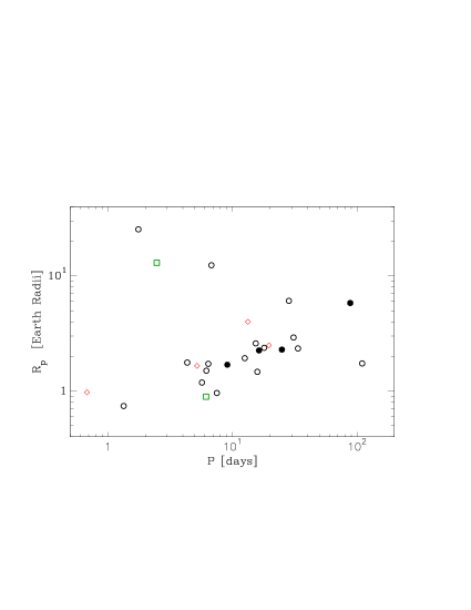
Figure 9: A period-radius plot for the confirmed planets in systems included in this study. Open circles are used for the systems in Table 3 judged to be CPM pairs, green squares indicate probable-CPM pairs, filled circles are drawn for LOS companions, and red diamonds indicate those systems for which no determination can be made at present.

In Figure 9, we show a period-radius relation for the confirmed exoplanets orbiting the stars in our current sample. The data are again taken from the Kepler CFOP website, where the radius values were then corrected for the dilution of the secondary star and the planet is assumed to orbit the primary. As Fulton et al. (2017) and other subsequent papers have shown, this plot contains a wealth of information relevant for planet formation and evolution. We have small sample statistics at present and the speckle observations do not represent a complete sample where observational biases can be fully accounted for; therefore, it would be unwise to over-interpret the plot as it stands, but a few initial comments can be made. First, the basic features of this plot, such as the major branch of data points following a trend toward smaller planetary radii as the period decreases and a lack of intermediate-sized planets with periods of less than 10 days, appear similar to the much larger sample of exoplanets orbiting single stars. Second, we do not yet have examples of planets in binary systems with radii exceeding 25$R_{\oplus}$, whereas the current known sample of exoplanets contains a well-defined sample of giant planets with radii at least as large as 40-50 $R_{\oplus}$. In an examination of planetary periods and radii with stellar properties such as mass and metallicity, no obvious trends were identified in our sample.

As with most of the Kepler discoveries, the planetary orbital periods are relatively short. Given the generally large separation of the binary pairs ($>$ 100 AU), these short-period planets are not likely to be greatly influenced by the presence of the stellar companion in the system. However, the planetary systems Kepler-449 and Kepler-907 are of potential interest in this regard due to the possibility of detecting orbital motion in the coming years. These planetary systems would be the most obvious candidates in this study with which to search for any dynamical effects the close stellar pairs may have on the currently known planets. Orbital resonances, inclination effects, or eccentric orbits may provide clues to gravitational influence by the bound companion, once enough high-quality astrometric data is obtained. Theoretical limits on additional outer planetary orbits might be explored as well.

The planets contained in large-separation binaries are all likely to orbit the primary star (Bouma et al., 2018), and the majority of the confirmed planets in our systems are of size 1-3 R_⊕. Kepler-1, -13, and -14 contain large, “Hot Jupiters” in close orbits, with migration possibly influenced by the bound companion. One of our CPM binary pairs, Kepler-449, has a motion consistent with an edge-on orbit, and would therefore be co-aligned with that of its planetary system. Continued observations of such systems, as well as others discovered by the K2 and TESS missions, is an important step in fully characterizing the motions and eventually determining binary orbits. That would give a unique viewpoint on understanding binary star and exoplanet system formation and evolution.

9 Conclusion

We have presented relative astrometry and photometry measurements obtained from speckle imaging for 57 KOIs over the time frame of 2010 to 2018, and performed a detailed study of 34 objects from the sample for which we have sufficient data to measure the relative proper motions of the system. Three of these systems are triple stars, and 18 of these systems have at least one confirmed exoplanet. Of those 18 exoplanet systems, we judge 12 to be either CPM or probable-CPM systems, and 2 to be LOS pairs. Four are of uncertain disposition based on our current measurements. Orbital periods for the confirmed planets in our sample range from 0.7 to 110 days, with a median period of 7.5 days. Our results are generally in agreement with the photometric analysis of Hirsch et al. (2017) where both studies were able to make determinations; the two exceptions are cases where the astrometry suggests a common proper motion but the earlier photometric analysis was not able to put the two stars on a common isochrone.

A preliminary period-radius relation for the confirmed exoplanets that are known in our sample reveals trends that comparable to the diagram for all exoplanets, including a lack of planets of radii comparable to Neptune at periods less than 10 days. This sample of Kepler CPM pairs hosting exoplanetary systems serves as a starting point for observational and theoretical development and speaks to the need for additional long-term astrometric observations. While the typical Kepler exoplanet host star is far away ($\sim$800 pc), we suggest that the same methodology presented here will provide a key tool that can be used on e.g. TESS stars in future years. As those stars are generally are much closer to the Solar system, shorter-period binary exoplanet host stars would be much more common and orbital motion would presumably be much more rapidly detected in those cases, and more robust statistics of a wider variety of exoplanet hosts may be obtained.

References

- Atkinson et al. (2017) Atkinson, D., Baranec, C., Ziegler, C, et al. 2017, AJ, 153, 25
- Bailer-Jones et al. (2018) Bailer-Jones, C. A. L., Rybiski, J., Fouesneau, M., Mantelet, G., & Andrae, R. 2018, AJ, 156, 58
- Bouma et al. (2018) Bouma, L. G., Masuda, K., & Winn J. N. 2018, AJ, 155, 244
- Ciardi et al. (2015) Ciardi, D., Beichman, C., Horch, E., & Howell, S. 2015, ApJ, 805, 16
- Désert et al. (2015) Désert, J., Charbonneau, D., Torres, G., et al. 2015, ApJ, 804, 59
- Everett et al. (2015) Everett, M. E., Barclay, T., Ciardi, D. R., et al. 2015, AJ, 149, 55
- Fulton et al. (2017) Fulton, B. J., Petigura, E. A., Howard, A. W., et al. 2017, AJ, 154, 109
- Furlan et al. (2017) Furlan, E., Ciardi, D. R., Everett, M. E., et al. 2017, AJ, 153, 2
- Furlan & Howell (2017) Furlan, E. & Howell, S. B. 2017, AJ, 154, 66
- Furlan & Howell (2020) Furlan, E. & Howell, S. B. 2020, ApJ, 898, 47
- Gaia Collaboration (2018) Gaia Collaboration 2018, A&A, 616, A1
- Hess et al. (2018) Hess, N. M., Thayer, P. R., Horch, E. P., et al. 2018, Proc. SPIE, 10701, 107012E
- Hirano et al. (2015) Hirano, T., Masuda, K., Sato, B., et al. 2015, ApJ, 799, 9
- Hirsch et al. (2017) Hirsch, L. A., Ciardi, D. R., Howard, A. M., et al. 2017, AJ, 153, 117
- Høg et al. (2000) Høg, E., Fabricius, C., Makarov, V. V., et al. 2000, A&A, 355, 27
- Horch et al. (2017) Horch, E. P., Casetti-Dinescu, D. I., Camarata, M. A. et al. 2017, AJ, 153, 212
- Horch et al. (2011) Horch, E. P., Gomez, S. C., Sherry, W. H., et al. 2011, AJ, 141, 45
- Horch et al. (2014) Horch, E. P., Howell, S. B., Everett, M. E., Ciardi, D. R., 2014, ApJ, 795, 60
- Horch et al. (2012) Horch, E. P., Howell, S. B., Everett, M. E., & Ciardi, D. R., 2012, AJ, 144, 165
- Horch et al. (2019) Horch, E. P., Tokovinin, A., Weiss, S. A., et al. 2019, AJ, 157, 56
- Horch et al. (2009) Horch, E., Veillette, D., Gallé, R., Shah, S., O’Rielly, G., Van Altena, W., 2009, 137, 5057
- Horch et al. (1996) Horch, E., Dinescu, D., Gerard, T., van Altena, W., Lopez, C., Franz, O. 1996, 111, 1681
- Horch et al. (2014) Horch, E. P., van Belle, G. T., Davidson, Jr., J. W., et al. 2015, AJ, 150, 151
- Howell et al. (2011) Howell, S. B., Everett, M. E., Sherry, W., Horch, E. P., & Ciardi, D. R. 2011, AJ, 142, 19
- Howell et al. (2019) Howell, S. B., Scott, N. J., Matson, R. A., Horch, E. P., & Stevens, A. 2019, AJ, 158, 113
- Kervella et al. (2019) Kervella, P., Gallenne, A., Remage Evans, N., et al. 2019, A&A, 623, A117
- Kraus et al. (2016) Kraus, A. L., Ireland, M. J., Huber, D., Mann, A. W., & Dupuy, T. J. 2016, AJ, 152, 8
- Kroupa (2001) Kroupa, P. 2001, MNRAS, 322, 231
- Lee et al. (2020) Lee, Y.-N., Offner, S. S. R., Hennebelle, P., et al. 2020, Space Science Reviews, 216, 70
- Lohmann, Weigelt, & Wirnitzer (1983) Lohmann, A. W., Weigelt, G., & Wirnitzer, B. 1983, Applied Optics, 22, 4028
- Matson et al. (2018) Matson, R. A., Howell, S. B., Horch, E. P., & Everett, M. E. 2018, AJ, 156, 31
- Mayo et al. (2018) Mayo, A. W., Vandenburg, A., Latham, D. W., et al. 2018, AJ, 155, 136
- Meng et al. (1990) Meng, J., Aitken, G., Hege, K., & Morgan, J. 1990, JOSAA, 7, 1243
- Pickles (1998) Pickles, A. J. 1998, PASP, 110, 749
- Raghavan et al. (2010) Raghavan, D., Mcalister, H. A., Henry, T. J., et al. 2010, ApJS, 190, 1
- Schmidt-Kaler (1982) Schmidt-Kaler, T. 1982, in Landolt-Börnstein New Series, Group 6, Vol. 2b, Stars and Star Clusters, ed. K. Schaefers and H.-H. Voigt (Berlin: Springer), 1
- Scott et al. (2018) Scott, N. J., Howell, S. B., Horch, E. P., & Everett, M. E. 2018, PASP, 130, 054502
- Torres et al. (2017) Torres, G., Kane, S. R., Rowe, J. F., et al. 2017, AJ, 154, 264
- Wang et al. (2014) Wang, J., Fischer, D. A., Xie, J.-W., & Ciardi, D. R. 2014, ApJ, 791, 111
- Wang et al. (2015a) Wang, J., Fischer, D. A., Horch, E. P., & Xie, J.-W. 2015, ApJ, 806, 130
- Wang et al. (2015b) Wang, J., Fischer, D. A., Xie, J.-W. & Ciardi, D. R. 2015, ApJ, 813, 130
- Wenger et al. (2000) Wenger, M., Ochsenbein, F., Egret, D. et al. 2000, A&AS, 143, 9
- Wittrock (2016) Wittrock, J., Kane, S. R., Horch, E. P., et al. 2016, AJ, 152, 149
- Youdin (2011) Youdin, A., 2011, ApJ, 742, 38
- Zacharias et al. (2013) Zacharias, N., Finch, C., Girard, T., et al. 2013, AJ, 145, 44
- Zielger et al. (2018) Ziegler, C., Law, N. M., Baranec, C., et al. 2018, AJ, 156, 83
- Ziegler et al. (2020) Ziegler, C., Tokovinin, A., Briceño, C., et al. 2020, AJ, 159, 19