Adversarial Black-Box Attacks On Text Classifiers Using Multi-Objective Genetic Optimization Guided By Deep Networks

Abstract

We propose a novel genetic-algorithm technique that generates black-box adversarial examples which successfully fool neural network based text classifiers. We perform a genetic search with multi-objective optimization guided by deep learning based inferences and Seq2Seq mutation to generate semantically similar but imperceptible adversaries. We compare our approach with DeepWordBug (DWB) on SST and IMDB sentiment datasets by attacking three trained models viz. char-LSTM, word-LSTM and elmo-LSTM. On an average, we achieve an attack success rate of $65.67\%$ for SST and $36.45\%$ for IMDB across the three models showing an improvement of $49.48\%$ and $101\%$ respectively. Furthermore, our qualitative study indicates that $94\%$ of the time, the users were not able to distinguish between an original and adversarial sample.

1 Introduction

Deep Neural Networks (DNNs) have witnessed tremendous success in day to day applications like chat-bots and self-driving vehicles. This has made it imperative to test the robustness of these models prior to their deployment for public consumption. Szegedy et al. (2013) first demonstrated the vulnerability of DNNs in computer vision by strategically fabricating adversarial examples. These carefully curated examples remain correctly classified by a human observer but can fool a targeted model.

Adversarial generation can be broadly classified into two types based on their access to the model. The generation algorithms that rely on the model internals are known as white-box algorithms Papernot et al. (2017); Kurakin et al. (2016); Baluja and Fischer (2017). Others Su et al. (2019); Sarkar et al. (2017); Cisse et al. (2017) which work without any knowledge about the model parameters and gradients are known as black box algorithms and are more prevalent in real-world scenarios. These works triggered a flurry of research towards i) evaluating the vulnerability of DNNs by attacking them with unperceivable perturbations, ii) measuring sensitivity and iii) developing defense mechanisms against such attacks. As industry increasingly employs DNN models in NLP tasks like text classification, sentiment analysis and question answering, such systems are also under the threat of adversaries Zhao et al. (2019); Horton (2016).

Existing adversarial techniques used to misguide image-based systems cannot be applied to text based systems because of two key reasons. First, image pixel values are continuous whereas words are discrete tokens. Hence, small changes in pixel values go unnoticed but the same cannot be said for typos or misfit words. Second, due to its discrete nature, input words are mapped to a continuous space using word embeddings. Therefore, any gradient computation is done only on the embeddings and not directly on the input words. Hence, previous gradient based attacks like FGSM Goodfellow et al. (2014) are difficult to apply on text models. In addition to the above challenges, perturbations applied to original text should be carefully crafted so that the adversarial sample is still a) structurally similar: the user should not be able to find differences in a quick glance, b) semantically relevant: the generated sample should bear the same meaning as the source sample and c) grammatically coherent: the generated sample should look natural and be grammatically correct.

To generate text adversaries satisfying multiple criteria, we formulate a multi-objective optimization problem, that once solved, results in the generation of text samples with adversarial properties. Thus, we model adversarial generation as a natural search space selection problem where the best adversaries are selected from a pool of samples initialized by different techniques. This selection is based on multiple objectives, where each objective measures a desirable adversarial quality. The selected samples then further undergo mixing (reproduction) and slight modifications (mutation) to create even better adversaries. As this model resembles the biological process of evolution, we rely on genetic algorithms as a tool to solve this optimization problem. Our genetic algorithm works in tandem with a sophisticated SeqtoSeq model for mutation, embedding based word replacements, textual noise insertions and deep learning based objectives to ensure a good selection of candidate solutions.

In summary, we propose a novel multi-objective genetic optimization that works in tandem with deep learning models to generate text adversaries satisfying multiple criterion. We conduct an extensive quantitative and qualitative study to measure the quality of the text adversaries generated and compare them with DeepWordBug (DWB) Gao et al. (2018).

2 Existing Literature

Most black-box adversarial algorithms for text have been rule based or have used supervised techniques. Such attacks are generally applied at sentence, word and character granularities.

At the sentence granularity, Jia and Liang (2017) shows how the addition of an out-of-context sentence acts like an adversary for comprehension systems. However, these sentences are easily identifiable as out-of-context by human evaluators.

At the word granularity, perturbations are generally introduced by selective word replacements. Papernot et al. (2017) focuses on minimum word replacements for generating adversarial sentences. Alzantot et al. (2018) uses single-objective genetic algorithms to generate adversaries by replacing words with their synonyms at an attempt to preserve semantics. Sato et al. (2018) introduces direction vectors which associate the perturbed embedding to a valid word embedding from the vocabulary.

To target character based models, adversarial attacks focusing at a character level have also surfaced. Gao et al. (2018) suggests a method to introduce random character level insertions using nearest keyboard neighbours. Li et al. (2018) focuses on attacking with character and word level perturbations. They introduce misspellings which map to unknown tokens when the model refers to a dictionary. However, introducing numerous misspellings makes it very difficult to comprehend adversaries.

Multi-objective optimization has been effective for many applications like image-segmentation and generating speech adversaries for ASR systems Bong and Mandava (2010); Khare et al. (2018). Our multi-objective optimization algorithm leverages the use of both selective word replacements and character level error insertion strategies. But unlike other works that rely on simple heuristics, we ensure that the modifications we make are essential and minimal by infusing guidance from deep learning based objectives. Guided by networks like Infersent Conneau et al. (2017), OpenAI GPT Radford (2018) and SeqtoSeq Bahdanau et al. (2014), we create adversaries that are structurally similar, semantically relevant and grammatically coherent.

3 Proposed Approach

Multi-objective optimization is the process of optimizing multiple objective functions Coello et al. (2006). The interaction among different objectives gives rise to a set of compromised solutions known as Pareto-optimal solutions Fonseca and Fleming (1995). Evolutionary algorithms are one class of popular approaches to generate such Pareto-optimal solutions.

Inspired from evolutionary systems, we consider adversarial text generation as an evolutionary process to generate adversarial samples satisfying multiple criteria. Carefully designed deep learning objectives and text processing algorithms assist in creating improved candidate solutions (text-samples) for fooling the classifier. Further, we propose various metrics to assess the fitness of a candidate (text-sample) within a population. After multiple generations, we finally apply heuristics to pick the most appropriate adversary that satisfies the desired adversarial properties discussed in the introduction.

An overview of the proposed algorithm for producing adversarial text samples for a given input is shown in Algorithm $1$. The entire process is divided into six main stages typical to an evolutionary process: i) Population Initialization, ii) Mutation, iii) Fitness Evaluation iv) Mating Pool Identification, v) Crossover and vi) Dominance Evaluation.

Our algorithm supports two ways of fooling classifiers. 1) Selectively substituting words with semantically equivalent terms. 2) Combining substitution of selective words along with introduction of typographical errors. We refer to these two modes of attacks as $Attack_{Single}$ and $Attack_{Combined}$ respectively. We report the results for both the types in the experiments section. The flow of the algorithm across the $6$ stages can be seen in Fig. 1 and lines $65$ to $94$ in Algorithm $1$. The details of each stage are explained in the following sections.

Algorithm 1 Algorithm for generating an adversarial text sample, given a reference input sample

1:$t_{Orig}\leftarrow$ Sample text,$w_{cf}\leftarrow$ Counter-Fitted Vectors, $popsize\leftarrow 64$

2:$Enc$, $Dec\leftarrow$ Encoder, Decoder of Sequence Mutator, $\delta{}\leftarrow 0.6$

3:$Mode_{Attack}\leftarrow$ 1 strategy from [$Attack_{Single}$, $Attack_{Combined}$]

4:

5:procedure Mutation($Sents,Mode_{Mutation}$)

6:     % Performs mutation in a Sentence %

7:     if  $Mode_{Mutation}$ is $Typo$  then

8:         % Add Typo in a Sentence %

9:         $muts\leftarrow AddTypo(Sents)$

10:     else

11:         % Pass Sentence through Sequence Mutator %

12:         $muts\leftarrow Dec(Enc(Sents))$      

13:return $muts$

14:

15:procedure Initialization($t_{Orig},Mode_{Mutation},popsize$)

16:     % Initialize the Population %

17:     $P\leftarrow list[]$

18:     Find important words $w_{imp}$ in $t_{Orig}$ using $Infer$

19:     Find substitute words $w_{sub}$ for the $w_{imp}$ with nearest neighbour search

20:     Allow only synonyms from $w_{sub}$ using $w_{cf}$ to ensure $similarity>\delta{}$

21:

22:     % Find all combinations of substitutions and create sentences %

23:     $combinations\leftarrow powerset(w_{sub})$

24:     for $w\in combinations$ do

25:         Apply $w$ in $t_{Orig}$ and add to $P$      

26:     $Pop\leftarrow popsize$ samples from $P$

27:     $Pop\leftarrow Mutation(P,Mode_{Mutation})$

28:return $Pop$

29:

30:procedure Fitness Evaluation($Population$)

31:     $set\leftarrow\{\}$

32:     Store fitness scores for $Population$ using Eqn. (1) to (5) in $set$.

33:return $set$

34:

35:procedure GetDominating($Population$, $popsize$)

36:     % Use the NSGA-2 Algorithm to select from Parents and Children %

37:     $P\leftarrow SelectNSGA2(Population,popsize)$

38:return $P$

39:

40:procedure Mating Pool($Parents,Fitness$)

41:     % List of Fittest Parent Pairs for Reproduction %

42:     $pool\leftarrow TournamentSelection(Parents,Fitness)$

43:return $pool$

44:

45:procedure Crossover($ParentPairs$)

46:     $set\leftarrow\{\}$

47:     for $p1,p2$ in $ParentPairs$ do:

48:         % Perform Crossover amongst normal forms %

49:         $c1,c2\leftarrow SinglePoint(p1.Ind,p2.Ind)$

50:

51:         % Perform Crossover amongst mutated forms %

52:         $c3,c4\leftarrow SinglePoint(p1.IndMut,p2.IndMut)$

53:         $set\leftarrow set\cup\{c1,c2,c3,c4\}$      

54:return $set$

55:

56:procedure GA($Population_{Old},Fitness_{Old},Mode_{Mutation}$)

57:     % Performs 1 iteration of the Genetic Algorithm %

58:     $parents\leftarrow MatingPool(Population_{Old},Fitness_{Old})$

59:     $children\leftarrow Crossover(parents)$

60:     $children\leftarrow Mutation(children,Mode_{Mutation})$

61:     $Population_{New}\leftarrow GetDominating(parents\cup children)$

62:     $Fitness_{New}\leftarrow FitnessEvaluation(Population_{New})$

63:return $Population_{New}$,$Fitness_{New}$

64:

65:procedure GA-Execute($t_{Orig},popsize,Mode_{Attack}$)

66:     if $Mode_{Attack}$ is $Attack_{Single}$ then

67:         % Complete population has only word swaps %

68:         ${P_{S}}_{i}\leftarrow Initialization(t_{Orig},Swaps,popsize)$

69:         ${F_{S}}_{i}\leftarrow FitnessEvaluation({P_{S}}_{i})$

70:     else

71:         % Half population ($P_{S}$) has only word swaps %

72:         ${P_{S}}_{i}\leftarrow Initialization(t_{Orig},Swaps,popsize//2)$

73:         ${F_{S}}_{i}\leftarrow FitnessEvaluation({P_{S}}_{i})$

74:

75:         % Half population ($P_{T}$) has word swaps with typos %

76:         ${P_{T}}_{i}\leftarrow Initialization(t_{Orig},Typos,popsize//2)$

77:         ${F_{T}}_{i}\leftarrow FitnessEvaluation({P_{T}}_{i})$      

78:

79:     % Perform GA multiple times %

80:     repeat

81:         if $Mode$ is $Attack_{Single}$ then

82:              % Perform an iteration of GA on the whole population %

83:              ${P_{S}}_{i+1},{F_{S}}_{i+1}\leftarrow GA({P_{S}}_{i},{F_{S}}_{i},Swaps)$

84:              ${P_{Total}}_{i+1}={P_{S}}_{i+1}$

85:         else

86:              % Perform an iteration of GA on the word swaps population %

87:              ${P_{S}}_{i+1},{F_{S}}_{i+1}\leftarrow GA({P_{S}}_{i},{F_{S}}_{i},Swaps)$

88:

89:              % Perform 1 iteration of GA on the typo population %

90:              ${P_{T}}_{i+1},{F_{T}}_{i+1}\leftarrow GA({P_{T}}_{i},{F_{T}}_{i},Typos)$

91:              ${P_{Total}}_{i+1}={P_{S}}_{i+1}\cup{P_{T}}_{i+1}$          

92:     until  ${P_{Total}}_{i+1}=={P_{Total}}_{i}$ or $i>maxiters$

93:return ${P_{Total}}_{i+1}$

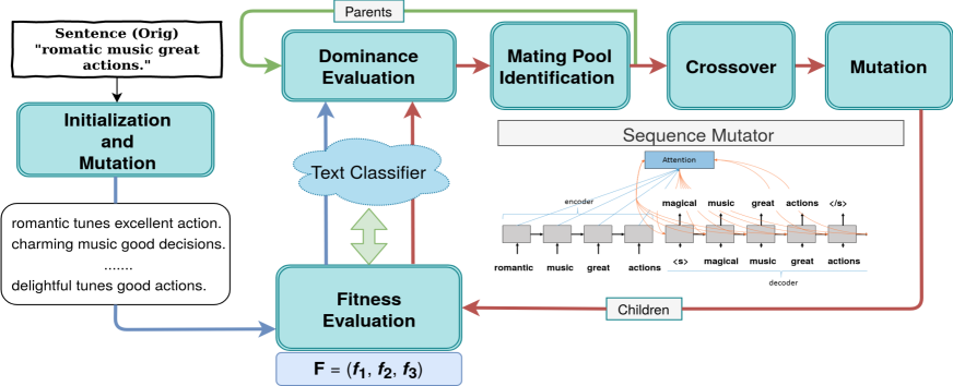
Figure 1: Adversarial Generation System using Multi-objective Genetic Algorithm

3.1 Initialization

In this phase (Algorithm $1$, Lines $15$-$28$), candidate samples in the population are initialized. For each sample, we lowercase and remove punctuation from the original text and perform word-level perturbations. These perturbations are done by first identifying the most important words in the text and then replacing them with semantically equivalent terms. To find the important words in the text, we max-pool the penultimate layer of the InferSent Model, which has been trained as a universal sentence encoder. Once the most important words are identified, we search for their nearest neighbours in the GloVe embedding space Pennington et al. (2014). This is done by finding similar vectors having cosine similarity more than $\delta{}$ (a hyper-parameter). We leverage the FAISS toolkit Johnson et al. (2017) for this step. To make sure that these neighbours are synonyms, we also verify that the cosine similarity is more than $\delta{}$ even in the counter-fitted vector space Mrkšić et al. (2016).

After finding the possible substitutions, we then initialize a population of candidate samples with all the possible combinations of original and substituted words. From this population, a small subset is selected randomly to make the genetic computation tractable. This careful initialization maintains diversity in the population and seeding it with original text guarantees faster convergence.

3.2 Mutation

The diversity of the existing population is further enhanced by mutation. In the text space, the mutation of a candidate is defined as a suitable word substitution. We rely on $2$ main approaches for substitutions 1) GloVe Mutator - a nearest neighbour search in the counter-fitted vector space as mentioned in the initialization phase and 2) Sequence Mutator - an encoder-decoder deep learning model to perform mutations in a sentence.

The Sequence Mutator is trained as a sequence to sequence bi-directional LSTM model with attention for the sole objective of predicting the same input that is fed to it. Hence the Sequence Mutator is made to iteratively predict a word given its left and right context in the input sentence until all the words in the input sentence are predicted.

This training objective makes the Sequence Mutator very similar to a language model. However, a key difference between the two, is the initial state supplied to the decoder. In a language model, the initial state is generally a vector of zeros, however, in the Sequence Mutator it is the context vector passed by the encoder. This context vector helps in copying the input sentence effectively. We perform beam search to get the top $5$ predictions from the Sequence Mutator. This step helps to randomly sample a mutated form of the input sentence.

In general, it is observed that the most probable prediction made by the Sequence Mutator is the original sentence itself and the remaining $4$ predictions are similar sentences with $1$ or $2$ words substituted probabilistically during decoding. We use the fairseq toolkit Ott et al. (2019) for fast prototyping of sequence to sequence model architectures.

It is very important to note that in the case of $Attack_{Single}$, we pass the entire population through the Sequence Mutator or Glove Mutator, whereas, in the case of $Attack_{Combined}$, we pass half of the population through the Sequence Mutator or Glove Mutator and for the other half we introduce typographical errors (Algorithm $1$, Lines $66$-$77$).

For typographical errors, we randomly select one or multiple words wherein the maximum number of words selected are less than $10$% of the length of the sentence. For the selected words, only $1$ of the following ways of typographical error introduction is chosen. i) Character swaps Soni and Lin (2019) and ii) QWERTY character map exchanges Pruthi et al. (2019). Character swaps are implemented by randomly choosing a character from the word and then swapping its place with an adjacent character. For the QWERTY character map exchange, the first step is to maintain a list of the adjacent symbols for every character in the QWERTY keyboard. When a character is randomly chosen, it is replaced by any one of the adjacent symbols. Both errors are included keeping in mind that they constitute a large portion of the most common typographical errors made while typing.

These steps are outlined in Algorithm $1$ (Lines $5$-$13$). To ensure diversity, we maintain both the normal and mutated forms of each candidate in the population. In Algorithm $1$, the normal and mutated forms of a candidate individual are denoted as $Ind$ and $IndMut$ respectively.

3.3 Fitness Evaluation

In-order to generate better candidate samples in the next generation, we need to identify the fittest candidates from the current population. The fitness function (Algorithm $1$, Lines: $30$-$33$) evaluates the adversarial nature of the samples i.e. the structural similarity, the semantic relevance and the ability to fool the target classification model. The fitness function for each candidate is a $3$ element vector $\vec{F}$.

$$\vec{F}=(f1,f2,f3)$$ (1)

The first objective value $f1$ measures the absolute change in the posterior probabilities when an individual candidate ($Ind$) and when the original text ($Orig$) are fed to the classifier ($Model$).

$$f1=abs(Model(Ind)-Model(Orig))$$ (2)

The second objective value measures the structural similarity between $Ind$ and $Orig$. This is calculated by finding the positional jaccard co-efficient between the $2$ sentences. As shown in Fig. 2, the intersection is $2$ words and the union is $6$ words. Hence, $PosJaccard=1/3$.

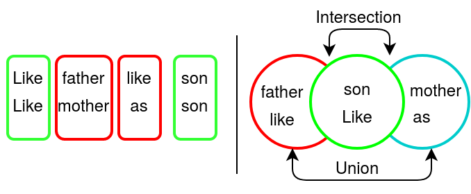
Figure 2: Positional Jaccard

$$PosJaccard(A,B)=|A|\cap|B|/|A|\cup|B|$$ (3)

$$f2=PosJaccard(Ind,Orig)$$ (4)

The third and final objective value measures the semantic relevance between $Ind$ and $Orig$. For this, we use the InferSent model to encode the sentences to fixed size vectors after which the cosine similarity is calculated.

$$f3=Sim(\vec{Infer(Orig)},\vec{Infer(Ind)})$$ (5)

In this manner, we incorporate each adversarial quality as an objective value derived from a deep learning model. By doing so, we ensure that only adversaries that have high structural similarity and semantic relevance progress to later iterations and form a major portion of the gene pool.

3.4 Mating Pool Identification

Once we calculate all the fitness functions, we then identify the fittest parents from the population. This step (Algorithm $1$, Lines: $40$-$43$) conducts a tournament selection to choose parents that will further undergo a crossover operation to produce children. In this tournament, a candidate sample completely dominates another opponent if the sample is at least as good as the opponent across all objective values. If not, the tie breaker for the tournament is the crowding metric which is a sub-part of the NSGA-2 Deb et al. (2002) algorithm.

3.5 Crossover

To enhance diversity in the adversarial samples, crossover is performed among the parent candidates. For crossover (Algorithm $1$, Lines: $45$-$54$) between two parents, we use a single point structural crossover. A word index is chosen randomly and then parts of the text after the index are swapped between the $2$ samples. As each candidate sample has a normal and mutated form, we perform crossovers between normal and mutated forms separately. Hence $2$ candidate samples produce $4$ offsprings - $2$ from crossover of the normal forms and $2$ from crossover of the mutated forms.

3.6 Dominance Evaluation

After the creation of children we proceed to evaluate their objective values. Post this, we are left with two sets of populations - the first is the set of parents and the second is the set of children. To maintain a constant population size during adversarial generation, we need to choose the best candidates from the combined group containing both parents and children. For this (Algorithm $1$, Lines: $35$-$38$), we employ our selection algorithm based on NSGA-2 Deb et al. (2002). In its standard formulation NSGA-2 groups candidates together if and only if every candidate in the group is not better than every other candidate in that group across all the objective values. Within the same group, ranks are given to candidates based on crowding metrics. We find that on experimentation, the standard formulation is successful at selecting good quality adversaries from the population.

Generated Adversarial Examples	Classifier	Label Flip
SST : A cumbersome burdensome and cliche-ridden movie greased with every emotional device known to man.	word-LSTM	- to +
SST : Birot is a competent enough filmmaker but her story tale has nothing fresh or very exciting about it.	word-LSTM	- to +
SST : A taut, intelligent sensible psychological drama.	char-LSTM	+ to -
SST : Has it ever been possible to say that Williams has truly genuinely inhabited a character?	char-LSTM	- to +
SST : Like most Bond outings in recent years some of the stunts are so outlandish outrageous that they border on being cartoon-like.	elmo-LSTM	- to +
IMDB : caught the tail … dont see the shooting only adds to the chillness of the plot to see both child infant and adult alike struggle to comprehend scavenge and come to terms with the senseless inane shootings was at times overwhelming surprising and will admit that i shed quite.	elmo-LSTM	+ to -

Table 1: Adversaries generated using our algorithm for different classifiers. The blue text indicates perturbations.

3.7 Final Selection

This process of evolution is repeated until the last iteration ($60$ steps) is reached or until population convergence (Algorithm $1$, Lines: $79$-$93$). To measure the grammatical coherence of the candidate samples, we pass the adversaries through the OpenAI GPT language model (LM) Radford (2018) and calculate the word normalized perplexity loss for each of the adversaries. The lower the loss for a particular candidate sample the better its quality. In order to select the best adversarial candidate from the final population, it was essential to derive a metric that emphasized on the desired adversarial qualities. For a given candidate individual ($Ind_{i}$), we would prefer that it has higher structural similarity ($f2_{i}$) and higher semantic relevance ($f3_{i}$) while simultaneously having a lower word normalized perplexity ($LM_{i}$).

$$score_{i}=(f2_{i}*f3_{i})/(LM_{i})^{\alpha}$$ (6)

Using this intuition, the metric ($score_{i}$ with $\alpha=1.2$) was calculated for each adversary and the best scoring adversaries were chosen from the test sets of SST-2 and for $1000$ reviews from IMDB corpus. On a $K80$ GPU, each iteration takes $0.5$ seconds for Glove and $3$ seconds for the Sequence Mutator.

4 Experimental Results and Analysis

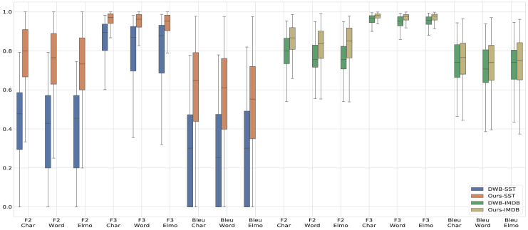
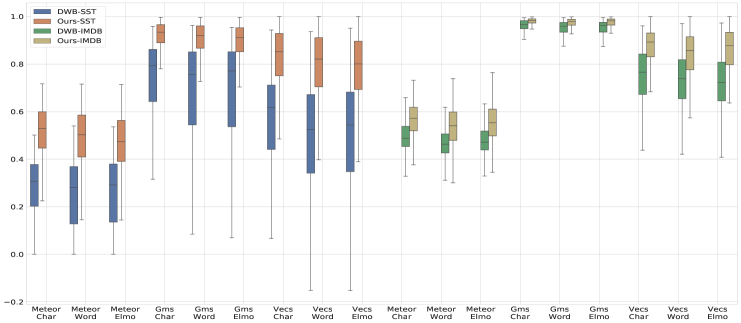
Figure 3: Metrics indicating semantic and structural similarity across adversarial and original sentences

Dataset	Classifier	Accuracy (Original)	Success Rate (Glove Mutator)		Success Rate (Seq2Seq Mutator)		DWB	Accuracy (Degraded)
-	-	-	$Attack_{Single}$	$Attack_{Combined}$	$Attack_{Single}$	$Attack_{Combined}$	(Success Rate)	Ours	DWB
SST	char-LSTM	75.26%	52.61%	70.75%	63.68%	73.67%	42.29%	26.33%	57.71%
	word-LSTM	82.95%	37.05%	61.35%	47.4%	63.52%	52.21%	36.48%	47.79%
	elmo-LSTM	87.02%	28.20%	57.72%	39.8%	59.82%	37.31%	40.18%	62.69%
IMDB	char-LSTM	87%	30.1%	37.5%	34.82%	39.5%	14.7%	60.5%	85.3%
	word-LSTM	90.4%	19.7%	41.3%	23.58%	42.7%	24.9%	57.3%	75.1%
	elmo-LSTM	92.34%	17.29%	26.19%	22.71%	27.15%	14.7%	72.85%	85.3%

Table 2: Success rate and Model performance degradation

Dataset	Classifier	AWR Metric		DWB			$Attack_{Combined}$ [Seq2Seq]
–	–	Ours	DWB	char-LSTM	word-LSTM	elmo-LSTM	char-LSTM	word-LSTM	elmo-LSTM
SST	char-LSTM	1.8	5.93	–	39.59%	43.17%	–	25.92%	19.55%
	word-LSTM	2.2	5.86	36.83%	–	49.19%	41.44%	–	32.41%
	elmo-LSTM	2.38	5.87	37.91%	56%	–	41.24%	44.37%	–
IMDB	char-LSTM	11.15	19.62	–	39.46%	34.69%	–	22.28%	21.27%
	word-LSTM	14.5	19.79	31.33%	–	40.56%	28.1%	–	26.93%
	elmo-LSTM	12.21	19.74	40.82%	53.06%	–	41.49%	46.89%	–

Table 3: AWR and Transferability of our adversaries in comparison to DWB. AWR : Average Words Replaced

4.1 Implementation Details

Classifiers: We studied the efficacy of our algorithm on 3 classifiers that consume text in unique ways - a word-LSTM model (word-tokens), a char-LSTM model (character-tokens) and an elmo-LSTM model (word and character tokens). Every model was trained on two sentiment datasets viz. Stanford Sentiment Treebank (SST-2) Socher et al. (2013) and IMDB movie reviews Maas et al. (2011). The char and word LSTMs were trained using the AllenNLP Gardner et al. (2017) toolkit. The elmo-LSTM was trained from scratch using a combination of Elmo Peters et al. (2018) and GloVe embeddings.
Sequence Mutator: We trained $2$ different instances of the Sequence Mutator - one for each dataset. In order to enhance its mutation capability, we train the mutator on a combined corpus of the test-set of the datasets and Wikitext-2 Merity et al. (2016). This allowed the mutator to be finetuned for the particular dataset but yet at the same time be exposed to a general natural language understanding. To ensure predictions were accurate, we windowed long sentences in the dataset into short groups of utmost $30$ words. To ensure a fast inference, we limited the model size to $4.9*10^{7}$ parameters. While training, we used a learning rate of $10^{-3}$ and eventually stopped the process when the average softmax cross-entropy loss of the model reached $0.05$ or below. Table 1 lists few adversarial samples generated by our approach.

In order to validate the efficacy of our algorithm, we generate adversaries for test-set inputs in SST and IMDB, and record the drop in accuracies for each classifier. As a baseline, we also attacked the $3$ classifiers with the current state of the art approach DeepWordBug (DWB) Gao et al. (2018).

4.2 Evaluation

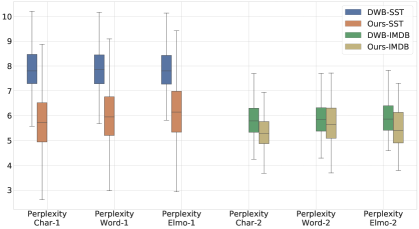
Figure 4: Perplexity Score

We performed both quantitative (Table 2) and qualitative (section 4.3) studies of our algorithm versus DWB. The study covers the following three dimensions - i) Performance degradation of the target models, ii) Transferability of adversarial samples across models, iii) Desired adversarial qualities in the generated samples.

The effect of adversarial text on a model is measured by the success rate and the decrease in model accuracy. Table 2 lists the original accuracy of the models, success rate of generated adversaries and the degraded accuracy of the models. There is a significant improvement over DWB across all the experiments. We also infer that our most successful strategy is the $Attack_{Combined}$ algorithm with a Sequence Mutator. On average, our success rate was $65.67\%$ for SST classifiers and $36.45\%$ for IMDB classifiers, where as, for DWB, it was only $43.93\%$ and $18.1\%$ respectively. As a result, there is a larger drop in accuracy when using our algorithm when compared to DWB as listed in Table 2. We also highlight the difference in success rates of the $Attack_{Single}$ mode with the Glove and Sequence mutator respectively. If one does not intend to allow typographical adversaries, there is a significant benefit in using the Sequence mutator.

Further, Table 3 shows the transferability of adversaries between the $3$ models. As shown, for the SST dataset, $41.44\%$ and $41.24\%$ of the adversaries curated for word-LSTM and elmo-LSTM respectively were transferable to char-LSTM. This clearly indicates that our attacks are transferable across models. As DWB aggressively introduces typographical errors in its adversaries, each typo maps to the unknown token irrespective of the classifier. Hence, as evident from Table 3, such adversaries are more transferable than those created by our approach. However, the increase in typos impact the quality of generated adversaries and affect its similarity with the original text.

This is further verified in Fig. 3 and Fig. 4, where we depict the distribution of various metrics that measure the quality of generated adversaries. We evaluate the adversaries using the objectives $f2$ and $f3$ along with natural language metrics like Blue, Meteor, Greedy matching score (GMS) and Vector extrema cosine similarity (VECS) Sharma et al. (2017). We obtain an average $f2$ value of $0.747$ for SST and $0.832$ for IMDB in comparison to DWB ($0.396$ and $0.756$ respectively). This $88.6\%$ increase for SST and $10.05\%$ increase for IMDB in $f2$ values indicates that we change far fewer words than DWB. This can be verified by the Average Words Replaced statistic in Table 3. We notice a similar trend for the $f3$ objective values as well. We also outperform DWB on word overlap metrics like Blue and Meteor. The Blue score for SST has a noticeably larger deviation for DWB when compared to our approach. Meteor mimics human judgment better than Blue by incorporating stemming and synonymy. We report higher Meteor scores in our generated adversaries signifying minimal perturbations. Similar improvements are noticed in sentence level metrics like VECS and GMS. VECS calculates the cosine similarity of sentence level embeddings whereas GMS calculates similarity scores between word embeddings and averages it for a sentence. Both of these sentence level metrics attain very high values with less deviation. These quantitative measures indicate that most of our adversaries enjoy high structural similarity and semantic relevance. In order to study the grammatical coherence of our adversaries, we also study the $LM$ scores in Fig. 4. We observe that our average $LM$ score for generated adversaries in SST and IMDB were $5.94$ and $5.5$ which is $24.1\%$ and $5.66\%$ lower in comparison to DWB ($7.83$ and $5.83$) signifying better grammatical coherence. All the quantitative measures suggest that our algorithm performs well at maximizing adversarial qualities in all generated adversaries. However, this is further validated by a qualitative study.

4.3 Qualitative Evaluation

We conducted a human evaluation study to determine if the generated adversaries were in reality visually imperceptible to humans. In order to assess the quality of the adversaries across various criteria, $34$ users (students and researchers from a computer science background) were presented with randomly sampled pairs of original and generated adversaries and then asked to answer multiple questions. We infer our insights from a total of $831$ data points obtained through this study.

Firstly, they were asked to predict the label of both the original and adversarial sample. $94\%$ of the users identified the same label for both the original and adversarial text indicating that adversarial samples remained unperceivable to users but were yet able to fool the model. Secondly, the users were asked whether the pairs had the same semantic meaning. $85\%$ of users identified them as semantically similar. This proved that the adversarial samples retained enough details from the reference and were semantically relevant. Finally, users were asked to rate the naturalness and grammatical correctness of each sample on a scale of $1-5$. The average score of $3.2$ for adversarial samples was very close to the score of $3.5$ for original samples which indicated that the adversarial samples were natural and grammatically coherent.

5 Conclusion and Future Work

We have successfully established that genetic algorithms can produce good quality adversaries if coupled with inference from deep learning based objectives and Seq2Seq mutation. Both the qualitative and quantitative evaluations indicate that most of the adversaries generated have desired adversarial qualities of structural similarity, semantic relevance and grammatical coherence.

The possible future directions for this work are i) Experimentation with algorithm sub-modules - During Initialization, LIME Ribeiro et al. (2016) based strategy can be used to select important words for perturbation. ii) Data Augmentation - We can study the performance of the classifiers when trained with these additional adversarial samples. iii) Expanding Attacks - We can study our performance on tasks like question answering, summarization etc.

References

- Alzantot et al. (2018) Moustafa Alzantot, Yash Sharma, Ahmed Elgohary, Bo-Jhang Ho, Mani Srivastava, and Kai-Wei Chang. 2018. Generating natural language adversarial examples. arXiv preprint arXiv:1804.07998.
- Bahdanau et al. (2014) Dzmitry Bahdanau, Kyunghyun Cho, and Yoshua Bengio. 2014. Neural machine translation by jointly learning to align and translate.
- Baluja and Fischer (2017) Shumeet Baluja and Ian Fischer. 2017. Adversarial transformation networks: Learning to generate adversarial examples. arXiv preprint arXiv:1703.09387.
- Bong and Mandava (2010) Chin-Wei Bong and Rajeswari Mandava. 2010. Multiobjective optimization approaches in image segmentation – the directions and challenges. International Journal of Advances in Soft Computing and Its Applications, 2.
- Cisse et al. (2017) Moustapha Cisse, Yossi Adi, Natalia Neverova, and Joseph Keshet. 2017. Houdini: Fooling deep structured prediction models. arXiv preprint arXiv:1707.05373.
- Coello et al. (2006) Carlos A. Coello Coello, Gary B. Lamont, and David A. Van Veldhuizen. 2006. Evolutionary Algorithms for Solving Multi-Objective Problems (Genetic and Evolutionary Computation). Springer-Verlag, Berlin, Heidelberg.
- Conneau et al. (2017) Alexis Conneau, Douwe Kiela, Holger Schwenk, Loïc Barrault, and Antoine Bordes. 2017. Supervised learning of universal sentence representations from natural language inference data. CoRR, abs/1705.02364.
- Deb et al. (2002) K. Deb, A. Pratap, S. Agarwal, and T. Meyarivan. 2002. A fast and elitist multiobjective genetic algorithm: Nsga-ii. Trans. Evol. Comp, 6(2):182–197.
- Fonseca and Fleming (1995) Carlos M. Fonseca and Peter J. Fleming. 1995. An overview of evolutionary algorithms in multiobjective optimization. Evolutionary Computation, 3(1):1–16.
- Gao et al. (2018) J. Gao, J. Lanchantin, M. L. Soffa, and Y. Qi. 2018. Black-box generation of adversarial text sequences to evade deep learning classifiers. In 2018 IEEE Security and Privacy Workshops (SPW), pages 50–56.
- Gao et al. (2018) Ji Gao, Jack Lanchantin, Mary Lou Soffa, and Yanjun Qi. 2018. Black-box generation of adversarial text sequences to evade deep learning classifiers. In 2018 IEEE Security and Privacy Workshops (SPW), pages 50–56. IEEE.
- Gardner et al. (2017) Matt Gardner, Joel Grus, Mark Neumann, Oyvind Tafjord, Pradeep Dasigi, Nelson F. Liu, Matthew Peters, Michael Schmitz, and Luke S. Zettlemoyer. 2017. Allennlp: A deep semantic natural language processing platform.
- Goodfellow et al. (2014) I. J. Goodfellow, J. Shlens, and C. Szegedy. 2014. Explaining and Harnessing Adversarial Examples. ArXiv e-prints.
- Horton (2016) Helena Horton. 2016. Microsoft deletes ‘teen girl’ai after it became a hitler-loving sex robot within 24 hours. The Telegraph, 24.
- Jia and Liang (2017) Robin Jia and Percy Liang. 2017. Adversarial examples for evaluating reading comprehension systems. arXiv preprint arXiv:1707.07328.
- Johnson et al. (2017) Jeff Johnson, Matthijs Douze, and Hervé Jégou. 2017. Billion-scale similarity search with gpus. ArXiv, abs/1702.08734.
- Khare et al. (2018) Shreya Khare, Rahul Aralikatte, and Senthil Mani. 2018. Adversarial black-box attacks on automatic speech recognition systems using multi-objective evolutionary optimization. In INTERSPEECH 2019.
- Kurakin et al. (2016) Alexey Kurakin, Ian Goodfellow, and Samy Bengio. 2016. Adversarial examples in the physical world. arXiv preprint arXiv:1607.02533.
- Li et al. (2018) Jinfeng Li, Shouling Ji, Tianyu Du, Bo Li, and Ting Wang. 2018. Textbugger: Generating adversarial text against real-world applications. arXiv preprint arXiv:1812.05271.
- Maas et al. (2011) Andrew L. Maas, Raymond E. Daly, Peter T. Pham, Dan Huang, Andrew Y. Ng, and Christopher Potts. 2011. Learning word vectors for sentiment analysis. In Proceedings of the 49th Annual Meeting of the Association for Computational Linguistics: Human Language Technologies - Volume 1, HLT ’11, pages 142–150, Stroudsburg, PA, USA. Association for Computational Linguistics.
- Merity et al. (2016) Stephen Merity, Caiming Xiong, James Bradbury, and Richard Socher. 2016. Pointer sentinel mixture models.
- Mrkšić et al. (2016) Nikola Mrkšić, Diarmuid Ó Séaghdha, Blaise Thomson, Milica Gašić, Lina M. Rojas-Barahona, Pei-Hao Su, David Vandyke, Tsung-Hsien Wen, and Steve Young. 2016. Counter-fitting word vectors to linguistic constraints. In Proceedings of the 2016 Conference of the North American Chapter of the Association for Computational Linguistics: Human Language Technologies, pages 142–148, San Diego, California. Association for Computational Linguistics.
- Ott et al. (2019) Myle Ott, Sergey Edunov, Alexei Baevski, Angela Fan, Sam Gross, Nathan Ng, David Grangier, and Michael Auli. 2019. fairseq: A fast, extensible toolkit for sequence modeling. In Proceedings of NAACL-HLT 2019: Demonstrations.
- Papernot et al. (2017) Nicolas Papernot, Patrick McDaniel, Ian Goodfellow, Somesh Jha, Z Berkay Celik, and Ananthram Swami. 2017. Practical black-box attacks against machine learning. In Proceedings of the 2017 ACM on Asia conference on computer and communications security, pages 506–519. ACM.
- Pennington et al. (2014) Jeffrey Pennington, Richard Socher, and Christopher Manning. 2014. Glove: Global vectors for word representation. In Proceedings of the 2014 Conference on Empirical Methods in Natural Language Processing (EMNLP), pages 1532–1543, Doha, Qatar. Association for Computational Linguistics.
- Peters et al. (2018) Matthew E. Peters, Mark Neumann, Mohit Iyyer, Matt Gardner, Christopher Clark, Kenton Lee, and Luke Zettlemoyer. 2018. Deep contextualized word representations. In Proc. of NAACL.
- Pruthi et al. (2019) Danish Pruthi, Bhuwan Dhingra, and Zachary C Lipton. 2019. Combating adversarial misspellings with robust word recognition. arXiv preprint arXiv:1905.11268.
- Radford (2018) Alec Radford. 2018. Improving language understanding by generative pre-training.
- Ribeiro et al. (2016) Marco Tulio Ribeiro, Sameer Singh, and Carlos Guestrin. 2016. ”why should I trust you?”: Explaining the predictions of any classifier. In Proceedings of the 22nd ACM SIGKDD International Conference on Knowledge Discovery and Data Mining, San Francisco, CA, USA, August 13-17, 2016, pages 1135–1144.
- Sarkar et al. (2017) Sayantan Sarkar, Ankan Bansal, Upal Mahbub, and Rama Chellappa. 2017. Upset and angri: breaking high performance image classifiers. arXiv preprint arXiv:1707.01159.
- Sato et al. (2018) Motoki Sato, Jun Suzuki, Hiroyuki Shindo, and Yuji Matsumoto. 2018. Interpretable adversarial perturbation in input embedding space for text. arXiv preprint arXiv:1805.02917.
- Sharma et al. (2017) Shikhar Sharma, Layla El Asri, Hannes Schulz, and Jeremie Zumer. 2017. Relevance of unsupervised metrics in task-oriented dialogue for evaluating natural language generation. CoRR, abs/1706.09799.
- Socher et al. (2013) Richard Socher, John Bauer, Christopher D. Manning, and Andrew Y. Ng. 2013. Parsing with compositional vector grammars. In Proceedings of the 51st Annual Meeting of the Association for Computational Linguistics (Volume 1: Long Papers), pages 455–465, Sofia, Bulgaria. Association for Computational Linguistics.
- Soni and Lin (2019) Devin Soni and Philbert Lin. 2019. Tool to generate adversarial text examples and test machine learning models against them. https://github.com/airbnb/artificial-adversary.
- Su et al. (2019) Jiawei Su, Danilo Vasconcellos Vargas, and Kouichi Sakurai. 2019. One pixel attack for fooling deep neural networks. IEEE Transactions on Evolutionary Computation.
- Szegedy et al. (2013) Christian Szegedy, Wojciech Zaremba, Ilya Sutskever, Joan Bruna, Dumitru Erhan, Ian J. Goodfellow, and Rob Fergus. 2013. Intriguing properties of neural networks. CoRR, abs/1312.6199.
- Zhao et al. (2019) Jieyu Zhao, Tianlu Wang, Mark Yatskar, Ryan Cotterell, Vicente Ordonez, and Kai-Wei Chang. 2019. Gender bias in contextualized word embeddings. arXiv preprint arXiv:1904.03310.