Spin Mode Reconstruction in Lagrangian Space

Abstract

Galaxy angular momentum directions (spins) are observable, well described by the Lagrangian tidal torque theory, and proposed to probe the primordial universe. They trace the spins of dark matter halos, and are indicators of protohalos properties in Lagrangian space. We define a Lagrangian spin parameter and tidal twist parameters and quantify their influence on the spin conservation and predictability in the spin mode reconstruction in $N$-body simulations. We conclude that protohalos in more tidal twisting environments are preferentially more rotation-supported, and more likely to conserve their spin direction through the cosmic evolution. These tidal environments and spin magnitudes are predictable by a density reconstruction in Lagrangian space, and such predictions can improve the correlation between galaxy spins and the initial conditions in the study of constraining the primordial universe by spin mode reconstruction.

I Introduction

The large scale structure (LSS) of the Universe contains plenty of cosmological information. One of the most important tasks of LSS studies is to use the distribution of galaxies to interpret the initial conditions of the Universe and cosmological parameters. The standard way is to relate the number density of galaxies in redshift space to the primordial density perturbation in Lagrangian space, including complications of survey geometries, biases of tracers and selection functions, redshift space distortion (RSD), nonlinear evolution and loss of cosmological information, etc.

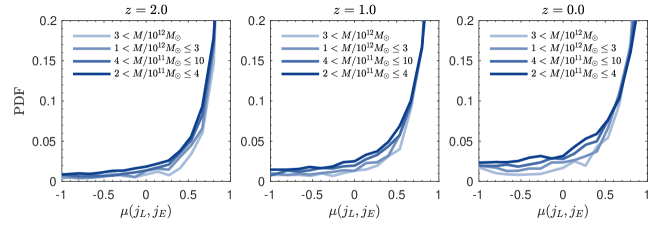
Figure 1: Conservation of the spin directions of dark matter halos shown by the probability distribution functions (PDFs) of $\mu(\boldsymbol{j}_{L},\boldsymbol{j}_{E})$ measured in different redshifts. The case of $\mu(\boldsymbol{j}_{L},\boldsymbol{j}_{E})=1$ corresponds to a fact that a halo and its protohalo have exact same spin directions, where the spin direction is maximumly conserved. $\mu$ obeys a tophat distribution between $-1$ and $1$ for uncorrelated vectors. In the three panels, the PDFs obviously departure from tophat distributions and suggest the conservation of halo spin. Curves with different colors represent the PDFs of $\mu(\boldsymbol{j}_{L},\boldsymbol{j}_{E})$ in different mass groups.

The rotation of galaxies adds another degree of freedom to probe the $B$-mode clustering of matter, and is proposed to provide additional information of the primordial universe. The tidal torque theory elucidates the basic mathematical framework that the initial misalignment between the moment of inertia of protohalos and the tidal fields they feel can produce persistent tidal torque 1969ApJ…155..393P ; 1970Afz…..6..581D ; 1984ApJ…286…38W . In SCDM (standard cold dark matter cosmology, a cosmological model without the cosmological constant, $\Omega_{m}=1,\Omega_{\Lambda}=0$) $N$-body simulations, 2000ApJ…532L…5L first quantified that this tidal torque is strongly correlated with the final halo spin and proposed using galaxy spins to reconstruct the initial tidal field 2001ApJ…555..106L . Although the spins of dark matter halos are not directly observable, hydrodynamic galaxy formation simulations all suggest that the spins of central galaxies and the spins of their host halos are highly correlated (e.g. 2015ApJ…812…29T and references therein). In Lagrangian space, by using the $E$-mode reconstructed density fields 2017PhRvD..95d3501Y we are able to construct a scale dependent spin mode, and successfully predict the spins of dark matter halos 2020PhRvL.124j1302Y . By applying this method to the ELUCID reconstruction of the local universe 2016ApJ…831..164W and a first spin catalog of observed galaxies, 2020NatAs.tmp..241M for the first time confirmed the correlation between galaxy spins and initial conditions of the Universe. These studies open the path of using galaxy spins to constrain the primordial state of the universe, including primordial non-Gaussianity, gravity waves, parity violation 2020PhRvL.124j1302Y , and neutrino mass 2019PhRvD..99l3532Y .

In order to maximize the constraining power, an important task is to understand galaxy spin - initial condition correlation as a function of many possible aspects: nonlinear evolution, quality of $E$-mode reconstruction, and galaxy types and their Lagrangian space properties. Besides the spin directions, the magnitude of the angular momentum vector has been extensively studied in many literatures, usually parameterized by spin parameters. The spin parameters characterize the rotation-supportedness of the dark matter halos in Eulerian space, and can not be directly measured since matter distribution and velocity dispersion of dark matter cannot be acquired simply through galaxy spectroscopy. A number of studies show that the morphologies of galaxies and galactic spin parameters are correlated 1983IAUS..100..391F ; 2012ApJS..203…17R (disk galaxies are rotation-supported as assumed in the classical disk galaxy formation model 1980MNRAS.193..189F ; 1998MNRAS.295..319M ). It is, however, not yet clear whether spin parameters of galaxies and their host halos are tightly correlated. Hydrodynamical cosmological hydrodynamical simulations (e.g., 2015MNRAS.449.2087D ; 2015MNRAS.450.2327Z ; 2020MNRAS.497.4346K ) suggested that spin parameters (also size) of galaxies are somewhat determined by initial angular momenta of their parent dark matter halos, but the correlation is possibly non-linear. Consistently, 2021arXiv210112373D showed somewhat signatures of correlation that halos having lower spin parameter are likely to form more compact galaxies in the IllustrisTNG simulations. 2019MNRAS.488.4801J , however, found a weak, if any, correlation using the galaxies from the NIHAO project. A method that can estimate the spin parameters of halos and protohalos sufficiently will permit us to predict the spins of galaxies better. As galaxy number densities and spins can be used to reconstruct the initial conditions in Lagrangian space, it is intuitive to study the Lagrangian properties of protohalos and protogalaxies and explore how they are related to the conservation and predictability of halo spins in Eulerian Space.

The rest of the paper is structured as follows. In Sec.II, we review the construction of the spin mode. In Sec.III, we define new spin parameters in Lagrangian space to qualify the misalignment between moment of inertia and tidal tensor. In Sec.IV, we present the results done by $N$-body simulations. Discussions and prospects are presented in Sec.V.

II Spin conservation and reconstruction

In this section we start with a numerical study of spin conservation while defining some of the key parameters. We use $j$ to denote the angular momentum of an object while use $L$ to denote any angular momentum fields. The Eulerian angular momentum vector of a dark matter halo is defined as $\boldsymbol{j}_{E}=\sum_{p}m_{p}(\boldsymbol{x}_{p}-\bar{\boldsymbol{x}})\times\boldsymbol{v}_{p}$, where $m_{p}$, $\boldsymbol{x}_{p}$ and $\boldsymbol{v}_{p}$ are the mass, Eulerian position and velocity of the $N$-body particles contained in a halo, and $\bar{\boldsymbol{x}}$ is its center of mass. Because the Lagrangian space coordinates can be identified by using particle-IDs, the Lagrangian space angular momentum vector is computed as

$$\boldsymbol{j}_{L}=\sum_{p}m_{p}\boldsymbol{q}_{p}^{\prime}\times\boldsymbol{u}_{p}=\sum_{p}m_{p}\boldsymbol{q}_{p}^{\prime}\times(-\nabla\phi|_{\boldsymbol{q}_{p}}),$$ (1)

where $\boldsymbol{q}_{p}$, $\bar{\boldsymbol{q}}$, $\boldsymbol{u}_{p}$ denote positions, center of mass, velocities in Lagrangian space, and $\boldsymbol{q}_{p}^{\prime}\equiv\boldsymbol{q}_{p}-\bar{\boldsymbol{q}}$. $\boldsymbol{u}_{p}$ is expressed by the gradient of the primordial gravitational potential $\phi$ 1970A&A…..5…84Z . We quantify the correlation between two spin directions as the cosine of their opening angle $\mu(\boldsymbol{v}_{1},\boldsymbol{v}_{2})=\cos\theta=\hat{\boldsymbol{v}}_{1}\cdot\hat{\boldsymbol{v}}_{2}\in[-1,1]$. In three-dimensional space, $\mu$ of two random (uncorrelated) vectors obeys a top-hat distribution with $\langle\mu\rangle=0$.

In a set of LSS $N$-body simulations generated by CUBE 2018ApJS..237…24Y , we identify dark matter halos by the friend of friend (FoF) method with the linking parameter $b=0.2$ at different redshifts. In Fig.1 we plot the probability distribution functions (PDFs) of $\mu(\boldsymbol{j}_{L},\boldsymbol{j}_{E})$ for different halo mass bins and redshifts. Here, the data is obtained from a flat $\Lambda$CDM simulation with cosmological parameters $\Omega_{m}=0.3,\Omega_{\Lambda}=0.7,\sigma_{8}=0.87,h=0.7$. A total of $512^{3}$ $N$-body particles are initialized at redshift $z_{\rm init}=100$ using the Zel’dovich approximation 1970A&A…..5…84Z and are evolved using the particle-particle particle-mesh (P3M) force calculation, in a periodic cubic box with $L=100\,{\rm Mpc}/h$ per side. The particle mass is thus $\simeq 8.8\times 10^{8}M_{\odot}$ and the least massive halos considered ($2\times 10^{11}M_{\odot}$) have $\simeq 230$ particles. The overall PDFs of $\mu(\boldsymbol{j}_{L},\boldsymbol{j}_{E})$ obviously depart from a tophat distribution, suggesting that $\boldsymbol{j}_{L}$, $\boldsymbol{j}_{E}$ directions are strongly correlated. The various PDF curves show the redshift and mass dependences. We can see that $\mu(\boldsymbol{j}_{L},\boldsymbol{j}_{E})$ tends to be higher for a fixed halo mass bin but at earlier epoch of the universe. For example, the expectation value $\langle\mu\rangle$ takes $0.78$, $0.71$ and $0.61$ for halos $10^{12}<M/M_{\odot}<3\times 10^{12}$, at redshifts 2.0, 1.0 and 0.0 respectively. Moreover, $\mu(\boldsymbol{j}_{L},\boldsymbol{j}_{E})$ is slightly higher for more massive halos at a fixed redshift.

To test the numerical convergence, we study $\mu(\boldsymbol{j}_{L},\boldsymbol{j}_{E})$ in a set of simulations with different mass and force resolutions. Mass resolutions are modified by smaller or larger box sizes but fixed grid and particle numbers, whereas force resolutions are configured by changing the grid number to particle number ratio, particle-partile force range etc. We find that higher mass or force resolution leads to only slightly higher $\mu(\boldsymbol{j}_{L},\boldsymbol{j}_{E})$ for given halo mass bins. For these reasons, we use the simulation configurations listed in the last paragraph and selected the lower halo mass bound to be $2\times 10^{11}M_{\odot}$ (230 $N$-body particles) so that the results in Fig.1 and in the rest of the paper converge and is reliable.

In the followings we use component equations involving vectors and tensors, and Einstein summation for repeated subscripts is implicitly assumed. Because the Lagrangian space corresponds to the initial, homogeneous state of the matter distribution, in Eq.(1) the sum over particles is equivalent to integration over $V_{q}$ – the protohalo region which eventually collapses into the halo. Further expanding the $-\nabla\phi$ term with respect to $\bar{\boldsymbol{q}}$ to the first order enables us to express the tidal torque prediction 1984ApJ…286…38W of $\boldsymbol{j}_{L}$ as

$$L_{IT} = \left.\int_{V_{q}}\epsilon_{ijk}q^{\prime}_{j}(-\phi_{,k}){\rm d}V\right|_{\text{1st-order}}$$ (2)

$$= \int_{V_{q}}\epsilon_{ijk}q^{\prime}_{j}\left(\left.-\phi_{,kl}\right|_{\bar{\boldsymbol{q}}}q^{\prime}_{l}\right){\rm d}V=\epsilon_{ijk}I_{jl}T_{lk},$$

where the 3D Levi-Civita symbol $\epsilon_{ijk}$ is used for the cross product in Eq.(1), and in the last equality the moment of inertia tensor of $V_{q}$ is defined as $(\mathbb{I})_{ij}=I_{ij}=\int_{V_{q}}q^{\prime}_{i}q^{\prime}_{j}{\rm d}V$ and the tidal tensor is defined as $(\mathbb{T})_{ij}=T_{ij}=-\phi_{,ij}$. From Eq.(2) we see that the $\boldsymbol{L}_{IT}$ field is a proxy of $\boldsymbol{j}_{L}$. Similar to Fig.1, we also confirmed the strong correlation in terms of $\mu(L_{IT},\boldsymbol{j}_{L})$ and $\mu(L_{IT},\boldsymbol{j}_{E})$ and they have similar mass and redshift dependences as $\mu(\boldsymbol{j}_{L},\boldsymbol{j}_{E})$. However, since $I_{ij}$ can not be obtained from the first principal, we are more interested in a predictable spin field given an initial density reconstruction. In 2020PhRvL.124j1302Y we construct a spin field from a “tide-tide” self-interaction $L_{TT}=\epsilon_{ijk}T^{r}_{jl}T^{R}_{lk}$ where $r$ and $R$ are two smoothing scales smoothed on the tidal tensor. Choosing Gaussian smoothing kernels with $R\rightarrow r_{+}$, the spin reconstruction can be approximated by

$$L_{TT}(r)=\epsilon_{ijk}\phi_{,jl}(r)\delta_{,lk}(r)$$ (3)

where $\delta$ is the initial overdensity field. We have confirmed that $\boldsymbol{L}_{TT}$ is a reconstructed spin field as a reliable proxy of $\boldsymbol{j}_{L}$, $\boldsymbol{j}_{E}$ of dark matter halos in $N$-body simulations 2020PhRvL.124j1302Y , of $\boldsymbol{j}_{E}$ of simulated galaxies in galaxy formation simulations (Liao et al. in prep.), and of $\boldsymbol{j}_{E}$ of observed disk galaxies 2020NatAs.tmp..241M .

III Spin parameters in Lagrangian space

So far we have discussed the spin correlations between $\boldsymbol{j}_{E}$, $\boldsymbol{j}_{L}$, $\boldsymbol{L}_{IT}$ and $\boldsymbol{L}_{TT}$ in terms of their directions. It is also intuitive to study the correlations between the magnitudes of these vectors. The spin magnitudes of dark matter halos have been extensively discussed. For example, a dimensionless spin parameter of a virialized object is defined as $\lambda_{P}\equiv J|E|^{1/2}G^{-1}M^{-5/2}$ 1969ApJ…155..393P or $\lambda_{B}\equiv J/(\sqrt{2}MVR)$ 2001ApJ…555..240B . Here $J$, $E$, $M$, $V$, $R$ are the total angular momentum, total energy, mass, circular velocity, radius of the system, and $G$ is the Newton’s constant. It is shown that $\lambda_{P}$ and $\lambda_{B}$ are similar for typical NFW halos 2001ApJ…555..240B , however not all the above quantities are straightforwardly defined for a protohalo in the Lagrangian space. Here we introduce some new parameters to characterize the spin magnitudes of Lagrangian halos. According to the kinematics of halo particles in Lagrangian space, a dimensionless kinematic spin parameter $\lambda_{K}$ can be defined as

$$\lambda_{K} \equiv \frac{\int_{V_{q}}\hat{j_{i}}\epsilon_{ijk}q^{\prime}_{j}u^{\prime}_{k}{\mathrm{d}}M}{\int_{V_{q}}q^{\prime}u^{\prime}{\mathrm{d}}M}=\frac{\int_{V_{q}}\sin\theta_{1}\cos\theta_{2}q^{\prime}u^{\prime}{\mathrm{d}}M}{\int_{V_{q}}q^{\prime}u^{\prime}{\mathrm{d}}M},$$ (4)

where $\hat{j_{i}}=(\boldsymbol{j}_{L}/j_{L})_{i}$ is the unit $\boldsymbol{j}_{L}$ vector ($j_{L}=|\boldsymbol{j}_{L}|$), $q^{\prime}=|{\boldsymbol{q}}^{\prime}|$, $u^{\prime}=|{\boldsymbol{u}}^{\prime}|$, $\sin\theta_{1}=\sqrt{1-\mu^{2}({\boldsymbol{q}}^{\prime},{\boldsymbol{u}}^{\prime})}$ and $\cos\theta_{2}=\mu(\boldsymbol{q}^{\prime}\times\boldsymbol{u}^{\prime},\boldsymbol{j}_{L})$. Clearly, $\lambda_{K}\in[0,1]$ characterizes the rotation-supportedness of the system. A coplanar system with all mass elements having homodromous circular orbits, $\lambda_{K}=1$, while a rotating rigid isodensity globe has $\lambda_{K}=8/3\pi\simeq 0.85$.

Similar to the fact that $\boldsymbol{L}_{IT}$ and $\boldsymbol{L}_{TT}$ being the proxies of $\boldsymbol{j}_{L}$ by the tidal torque theory, we can also find proxies of $\lambda_{K}$ in Lagrangian space. We expect that the rotation-supportedness $\lambda_{K}$ of a Lagrangian system depends on
(a) the anisotropies of the tidal field, (b) the nonspherical distribution of the protohalo, and (c) the misalignment between the principal axes of the above two. Both (a) and (b) can be characterized by the elipticity $e=(\lambda_{1}-\lambda_{3})/2(\lambda_{1}+\lambda_{2}+\lambda_{3})$ and prolateness $p=(\lambda_{1}-2\lambda_{2}+\lambda_{3})/2(\lambda_{1}+\lambda_{2}+\lambda_{3})$ of the tensors $\mathbb{I}$ and $\mathbb{T}$, where $\lambda_{1,2,3}$ are the primary, intermediate and minor eigenvalues of the tensor 2002MNRAS.332..339P . For (c) 2009ApJ…707..761L has defined an alignment parameter $\beta\equiv 1-\sqrt{(\varrho^{2}_{12}+\varrho^{2}_{23}+\varrho^{2}_{31})/(\varrho^{2}_{11}+\varrho^{2}_{22}+\varrho^{2}_{33})}$, where $\varrho_{ij}$’s are the re-expressions of elements of $\mathbb{I}$ in the principal frame of $\mathbb{T}$. We find weak correlations between $\lambda_{K}$ and these parameters. Here we define dimensionless parameters

$$\beta_{IT} \equiv \left.\frac{\left|\int_{V_{q}}\epsilon_{ijk}q^{\prime}_{j}u^{\prime}_{k}{\mathrm{d}}V\right|}{-\int_{V_{q}}q^{\prime}_{i}u^{\prime}_{i}{\mathrm{d}}V}\right|_{\text{1st-order}}$$ (5)

$$= \frac{\left|\int_{V_{q}}\epsilon_{ijk}q^{\prime}_{j}(-\phi_{,kl}q^{\prime}_{l}){\mathrm{d}}V\right|}{-\int_{V_{q}}q^{\prime}_{i}(-\phi_{,ij}q^{\prime}_{j}){\mathrm{d}}V}=\frac{\left|\epsilon_{ijk}I_{jl}T_{lk}\right|}{-I_{ij}T_{ij}}$$

and similarly

$$\beta_{TT}(r) \equiv =\frac{\left|\epsilon_{ijk}\phi_{,jl}(r)\delta_{,lk}(r)\right|}{-\phi_{,ij}(r)\delta_{,ij}(r)}$$ (6)

as the proxies of $\lambda_{K}$, where $\beta_{IT}$ optimizes the measurement of anisotropies and misalignment between two tensors $\mathbb{I}$ and $\mathbb{T}$, whereas tidal environment parameter $\beta_{TT}$ measures the anisotropy and twist of $\mathbb{T}$ on physical scale $r$. A schematic interpretation of $\beta_{TT}$ is discussed in the figure 1 of 2020NatAs.tmp..241M .

In the spin mode reconstruction 2020PhRvL.124j1302Y , in order to optimize the correlation $\mu(\boldsymbol{j}_{L},\boldsymbol{j}_{E})$, the smoothing scale $r$ is chosen to match the equivalent protohalo scale $r=r_{q}(M)=(2MG/\Omega_{m}H_{0}^{2})^{1/3}$, otherwise $\boldsymbol{j}_{L}$ and $\boldsymbol{j}_{E}$ are decorrelated. Here $\Omega_{m}$ is the density parameter for matter and $H_{0}$ is the Hubble constant.

IV Spin Conservation and Predictability

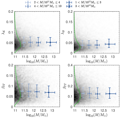
Figure 2: PDFs of $\lambda_{K}$, $\lambda_{B}$, $\beta_{\rm IT}$, $\beta_{\rm TT}$ and their halo mass dependences. The four green curves show the PDFs of these parameters and the gray scale maps represent the halo number density in the two-dimensional parameter space. The normalizations are arbitrarily set for a clear visualization. We partition all halos into four mass groups specified on the top of the figure, and inside each mass group, we take the three quartiles $\{Q_{1},Q_{2},Q_{3}\}$ of the parameter distribution as the lower/left boundary of the error bar, center of the error bar, and upper/right boundary of the error bar.

The following results are obtained from the $z=0$ checkpoint of a simulation described in Sec.II. The numerical convergence is also verified by using a set of companion simulations with different mass and force resolutions as mentioned in Sec.II

In Fig.2 we plot the PDFs of $\lambda_{K}$, $\lambda_{B}$, $\beta_{\rm IT}$, $\beta_{\rm TT}$ and their joint PDFs with halo mass. The green curves in the four panels show the PDFs of the indicated parameters for all halos with at least 100 particles ($>8.8\times 10^{10}M_{\odot}$), however we note that they are insensitive for selected halo mass bins. The Lagrangian space spin parameter $\lambda_{K}$ has a very similar distribution as $\lambda_{B}$. In particular, $\langle\lambda_{K}\rangle\simeq 0.063$ with a standard deviation $\sigma\simeq 0.041$, in comparison, $\langle\lambda_{B}\rangle\simeq 0.051$ with a standard deviation $\sigma\simeq 0.037$. All these parameters show a lognormal probability distribution, with the expectation value $\leq 0.1$. We use gray-scale color maps to show the two-dimensional PDFs of each parameter and halo mass. To clearly illustrate the mass dependences here and for the following studies, we select all halos which are more massive than $2\times 10^{11}M_{\odot}$, and partition them into four mass bins. Note that, due to the behaviour of the halo mass function, a significant portion of less massive halos are beyond the lower bound of the lowest mass bin, however whether including them does not change the statistics. For each mass bin, we plot the center of the error bar at the median of halo mass and the median of the parameter in consideration. The lower/left and upper/right boundary of each error bar are taken as the 25% and 75% percentiles of the distribution. Similar to that of $\lambda_{B}$, we do not see obvious mass dependences of other parameters in Fig.2.

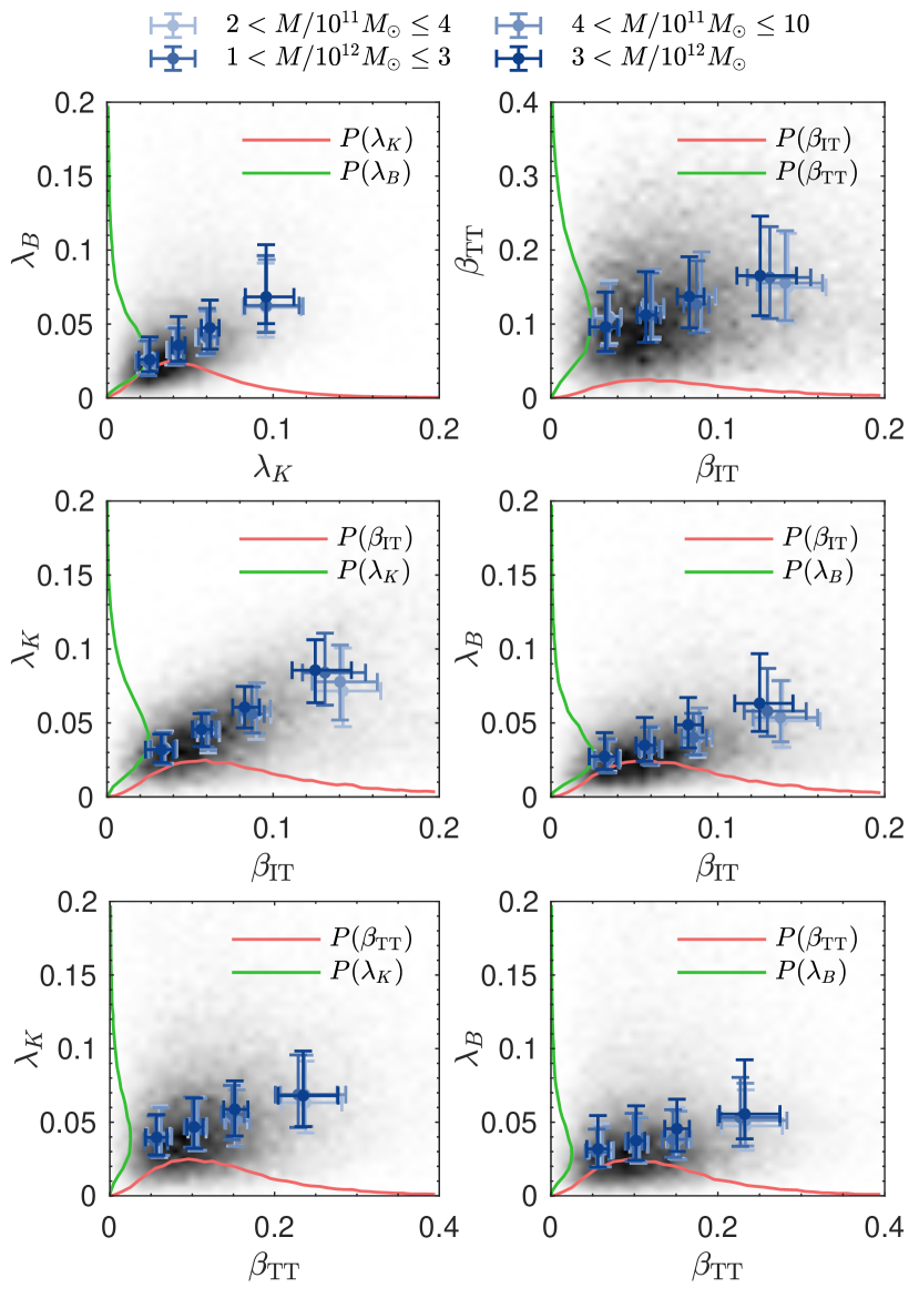
Figure 3: Dependences between $\lambda_{K}$, $\lambda_{B}$, $\beta_{\rm IT}$ and $\beta_{\rm TT}$. The gray scale in the background represents their distribution in two-dimensional parameter space, and halos are divided into four mass bins specified on the top of the figure. The red and green curves represent the PDFs of the parameters indicated by the label of each axis. The data are partitioned into four mass bins as shown on the top of the figure, and then are sorted by the value of parameters in the $x$-axis, with the positions and boundaries the same as Fig.2.

In Fig.3, we plot the dependences between $\lambda_{K}$, $\lambda_{B}$, $\beta_{IT}$ and $\beta_{TT}$ in six panels. For each pair of parameters we use the gray scale to plot the halo number densities in their two-dimensional parameter space, and the two curves show their individual PDF. Again, all halos are partitioned into four mass bins indicated, and the positions and boundaries of the error bars are determined similarly as Fig.2. A subtle difference is that, for each mass bin, the data are subsequently sorted according to the parameter in the horizontal axis ($\lambda_{K}$ in the top-left panel, for example) and then partitioned into four groups of equal (may differ up to one) number of halos. Then, for each group, the error bar position and boundaries are determined by the two parameters ($\lambda_{K}$ and $\lambda_{B}$ in the top-left panel, for example) in consideration. Thus there are 16 error bars in each panel, and we use gray scales of the error bar to indicate mass, and for each mass bin, the four groups are naturally placed horizontally. For all panels, we see positive correlations between all six possible combinations of four parameters despite of the certain scatters. Firstly, in the top-left panel, either by the 2D PDF or the error bars, we see a strong positive correlation between $\lambda_{K}$ and $\lambda_{B}$, and the correlation appears in all halo mass bins. It shows that the kinematic spin-supportedness of Lagrangian halos is closely related to the Eulerian spin parameter – a more spin supported Lagrangian protohalo is more likely to result in a spin supported halo at $z=0$. In the middle-left panel, the correlation between $\beta_{IT}$ and $\lambda_{K}$ shows that a more isotropic $\mathbb{I}$ and $\mathbb{T}$ and a more misalignment between the two indeed lead to a more spin-supported Lagrangian protohalo. The bottom-left and top-right panels show that $\beta_{TT}$ is indeed a proxy of $\beta_{IT}$ and $\lambda_{K}$, making the prediction of Lagrangian spin parameter applicable. Finally, the middle-right and bottom-right panels also illustrate positive correlations between $\beta_{IT}$ - $\lambda_{B}$ and $\beta_{TT}$ - $\lambda_{B}$ respectively, although the correlations are weaker compared to the correlations measured directly in Lagrangian space.

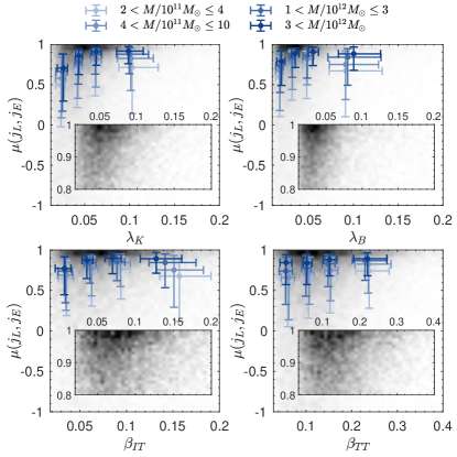
Figure 4: PDFs of $\lambda_{K}$, $\lambda_{B}$, $\beta_{\rm IT}$, $\beta_{\rm TT}$ and the spin conservation quantified by $\mu(\boldsymbol{j}_{L},\boldsymbol{j}_{E})$. The gray-scale color maps show the two-dimensional PDFs of each parameter and correlation function $\mu(\boldsymbol{j}_{L},\boldsymbol{j}_{E})$. The bottom right inset of each panel is the zoom-in PDF of the most dense part. The data are partitioned into four mass bins and sorted the same as Fig.3.

Next we investigate how the spin conservation depends on the spin parameters and Lagrangian properties. In Fig.4 we choose the horizontal axes as the $\lambda_{K}$, $\lambda_{B}$, $\beta_{\rm IT}$ and $\beta_{\rm TT}$ and the vertical axes as $\mu(\boldsymbol{j}_{L},\boldsymbol{j}_{E})$ and use the gray-scale maps to show the halo number densities on these parameter spaces. The error bars are plotted the same as in Fig.3. In the top-left panel, we clearly see that, in Lagrangian space, and for all the four mass bins, spin-supported (high-$\lambda_{K}$) protohalos tend to preserve their spin directions all the way to $z=0$, leading to a systematically higher $\mu(\boldsymbol{j}_{L},\boldsymbol{j}_{E})$. For these halos, the spins observed in Eulerian space contain more information if we directly use the Eulerian spin to study the primordial universe. In the top-right panel we see the same trend when the horizontal axis is replaced by $\lambda_{B}$, except that the highest $\lambda_{B}$ shows a slight decrease in $\mu(\boldsymbol{j}_{L},\boldsymbol{j}_{E})$ for all mass bins. In the bottom-left panel, $\mu(\boldsymbol{j}_{L},\boldsymbol{j}_{E})$ is also positively correlated with $\beta_{\rm IT}$, except for the three lowest mass bins, where the highest $\beta_{\rm IT}$ leads $\mu(\boldsymbol{j}_{L},\boldsymbol{j}_{E})$ to decrease. Most importantly, in the bottom-right panel, we see a consistent positive correlation between $\mu(\boldsymbol{j}_{L},\boldsymbol{j}_{E})$ and $\beta_{\rm TT}$ for all mass bins. $\beta_{\rm TT}$ can be directly calculated by the reconstructed initial density field, so in principle we can weight those halo-galaxy systems with high $\beta_{\rm TT}$ values such that their observed spins better reflect cosmological information in Lagrangian space.

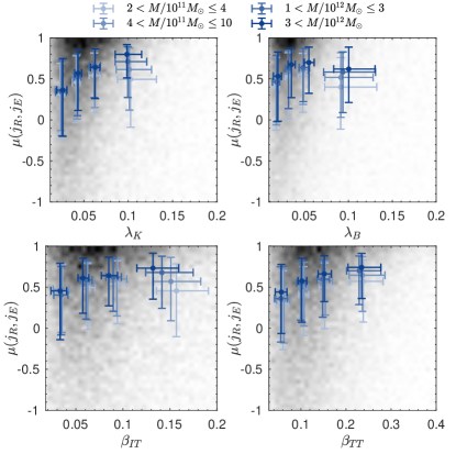
Figure 5: PDFs of $\lambda_{K}$, $\lambda_{B}$, $\beta_{\rm IT}$, $\beta_{\rm TT}$ and the spin conservation quantified by $\mu(\boldsymbol{j}_{R},\boldsymbol{j}_{E})$. The gray-scale color maps and error bars are the same as in Fig.4, except the horizontal axes are set as $\mu(\boldsymbol{j}_{R},\boldsymbol{j}_{E})$.

Next, we reconstruct the predicted halo spins by the Eq.(3) with the optimal smoothing scale $r=r_{\rm opt}=(2M_{\rm bin}G/\Omega_{m}H_{0}^{2})^{1/3}$, where $M_{\rm bin}$ is the averaged halo mass of the corresponding mass bin. In 2020PhRvL.124j1302Y we have demonstrated that a rough estimate of the halo mass can give accurate spin reconstruction, not sensitive to the mass estimation. The predicted halo spin is thus $\boldsymbol{j}_{R}=\boldsymbol{L}_{TT}(r_{\rm opt})$. The predictability of halo spins is quantified by $\mu(\boldsymbol{j}_{R},\boldsymbol{j}_{E})$. In Fig.5 we plot $\mu(\boldsymbol{j}_{R},\boldsymbol{j}_{E})$ as a function of parameters $\lambda_{K}$, $\lambda_{B}$, $\beta_{\rm IT}$ and $\beta_{\rm TT}$ similar to Fig.4. Compared to Fig.4, the dependences of $\mu(\boldsymbol{j}_{R},\boldsymbol{j}_{E})$ to $\lambda_{K}$, $\lambda_{B}$, $\beta_{\rm IT}$, $\beta_{\rm TT}$ show similar trends to that of $\mu(\boldsymbol{j}_{L},\boldsymbol{j}_{E})$ but with more dispersion in the distribution of spin predictability. Importantly, in the bottom right panel, we see positive correlation between $\beta_{TT}$ and $\mu(\boldsymbol{j}_{R},\boldsymbol{j}_{E})$ for all mass bins. From density reconstruction, we can calculate both $\beta_{TT}$ and $\boldsymbol{j}_{R}$ of each halo, and this correlation suggests that halos with higher $\beta_{TT}$ values tend to have more reliable predicted halo spins $\boldsymbol{j}_{R}$. So we can directly estimate the accuracy of spin reconstruction for all halos, and improve the accuracy of the reconstructed initial condition.

V Conclusion

We study the conservation and predictability of the angular momenta of dark matter halos depending on their spin parameters and Lagrangian space properties.

Similar to the definitions of halo spin parameters in Eulerian space, we construct a dimensionless kinematic spin parameter $\lambda_{K}$ of protohalos in Lagrangian space. Higher $\lambda_{K}$ corresponds to more rotational-supported systems. According to the tidal torque theory, we introduce the parameter $\beta_{\rm IT}$ to characterize the anisotropies of $\mathbb{I}$ and $\mathbb{T}$ and the misalignment between the two, where $\mathbb{I}$ is the moment of inertia tensor of the protohalo and $\mathbb{T}$ is the tidal tensor it feels. The kinematics of a low $\beta_{\rm IT}$ protohalo is more dominated by a radial convergence flow rather than coherent circular motions. Our simulations show that these low $\beta_{\rm IT}$ protohalos typically have low $\lambda_{K}$ and are eventually more likely to evolve into velocity dispersion supported (low $\lambda_{B}$) halos. Similar to the spin mode reconstruction in 2020PhRvL.124j1302Y , we also reconstruct the tidal torque scalar $\beta_{\rm TT}$ from initial density fields and it turns out that $\beta_{\rm TT}$ is a reliable proxy of $\beta_{\rm IT}$ to characterize the spin parameters.

We quantify the conservation of halo spins as the correlation between their Lagrangian and Eulerian spin directions $\mu(\boldsymbol{j}_{L},\boldsymbol{j}_{E})$. From simulations we see that rotation supported protohalos (higher $\lambda_{K}$, and thus statistically higher $\lambda_{B}$, $\beta_{\rm IT}$ and $\beta_{\rm TT}$) tend to better preserve their spin during the cosmic evolution, and result in a higher $\mu(\boldsymbol{j}_{L},\boldsymbol{j}_{E})$. This is understandable – for less rotation supported systems it is difficult to determine their total angular momentum vectors and the rather random $\boldsymbol{j}_{L}$ and $\boldsymbol{j}_{E}$ result in a random correlation between the two. We also show that the spin predictability by Eq.(3) 2020PhRvL.124j1302Y is positively correlated with these spin parameters.

The spins of disk galaxies are observable and we have discovered a positive correlation signal between disk galaxies and their halos and the reconstructed initial density field of the local universe 2020NatAs.tmp..241M . This observed correlation is a result of many facts: the observability of galaxy spiral arms indicating their spin directions; the underlying galaxy-halo spin correlation, confirmed by many galaxy formation simulations; the Lagrangian-Eulerian spin correlation; the tidal torque theory and spin mode reconstruction linking the primordial density field with protohalo spins; and the density reconstruction given galaxy positions. Galaxy spins are proposed to discover properties of the primordial universe such as neutrino mass, chiral violations, primordial non-Gaussianities etc, and a better understanding of the above facts and improve the correlations will be the first step. This paper shows that Lagrangian spin parameter $\lambda_{K}$ is closely related to Eulerian ones $\lambda_{B}$, and to the Lagrangian tidal properties, and is predictable. Therefore, a weighted selection of rotation-supported halos by $\beta_{TT}$ is expected to straightforwardly improve the spin correlation to the primordial universe.

The spin reconstruction algorithms consider dark matter halos and protohalos and do not include any baryonic effects. This is because we have used the Lagrangian space information, i.e., the primordial tidal environment properties, to predict the spin in the Eulerian space. The baryonic and dark matter components of a galaxy-halo system have very similar protovolumes in Lagrangian space 2017MNRAS.470.2262L , so they feel the same direction and magnitude of the initial tidal torque, which is constributed by the initial total gravity. This is the reason why the observation of galaxy spins are correlated with the dark matter (or total) initial conditions 2020NatAs.tmp..241M . This work uses dark matter only simulations and focuses on how spin parameters influence the spin conservation and predictability of dark matter halos. Since galaxy and halo spin directions are tightly correlated 2015ApJ…812…29T , better predictability of halo spin directions indicates better predictability of galaxy spin directions, so the spin parameters of protohalos are also related to the predictability of galaxy spin directions. Our method can also be applied to investigate the correlation of spin magnitudes between galaxies and their host halos, which is out of the scope of this paper.

The kinematic spin parameter can also be used to describe the rotation of cosmic filaments. The filament spins are confirmed by observations of the peculiar velocities of galaxies 2020ApJ…900..129W and by numerical simulations 2020arXiv200602418X . In Lagrangian space, the origin of the filament spin could also be described by the initial tidal field. On the other hand, the Eulerian filaments are non-virialized systems so we expect their spins correlated with Lagrangian ones. In both Eulerian and Lagrangian spaces, the spin magnitudes can be quantified by $\lambda_{K}$. Additionally, in cosmic filaments, it would be interesting to study the correlations between large scale spin mode by galaxy peculiar velocities and small scale spin modes by galaxy spins.

References

- (1) P. J. E. Peebles, ApJ155, 393 (1969).
- (2) A. G. Doroshkevich, Astrofizika 6, 581 (1970).
- (3) S. D. M. White, ApJ286, 38 (1984).
- (4) J. Lee and U.-L. Pen, ApJ532, L5 (2000), astro-ph/9911328.
- (5) J. Lee and U.-L. Pen, ApJ555, 106 (2001), astro-ph/0008135.
- (6) A. F. Teklu et al., ApJ812, 29 (2015), 1503.03501.
- (7) H.-R. Yu, U.-L. Pen, and H.-M. Zhu, Phys. Rev. D95, 043501 (2017), 1610.07112.
- (8) H.-R. Yu et al., Phys. Rev. Lett.124, 101302 (2020), 1904.01029.
- (9) H. Wang et al., ApJ831, 164 (2016), 1608.01763.
- (10) P. Motloch, H.-R. Yu, U.-L. Pen, and Y. Xie, Nature Astronomy (2020), 2003.04800.
- (11) H.-R. Yu, U.-L. Pen, and X. Wang, Phys. Rev. D99, 123532 (2019), 1810.11784.
- (12) S. M. Fall, Galaxy formation - Some comparisons between theory and observation, in Internal Kinematics and Dynamics of Galaxies, edited by E. Athanassoula, volume 100, pp. 391–398, 1983.
- (13) A. J. Romanowsky and S. M. Fall, ApJS203, 17 (2012), 1207.4189.
- (14) S. M. Fall and G. Efstathiou, MNRAS193, 189 (1980).
- (15) H. J. Mo, S. Mao, and S. D. M. White, MNRAS295, 319 (1998), astro-ph/9707093.
- (16) M. Danovich, A. Dekel, O. Hahn, D. Ceverino, and J. Primack, MNRAS449, 2087 (2015), 1407.7129.
- (17) A. Zolotov et al., MNRAS450, 2327 (2015), 1412.4783.
- (18) M. Kretschmer, O. Agertz, and R. Teyssier, MNRAS497, 4346 (2020), 2003.03368.
- (19) M. Du et al., arXiv e-prints , arXiv:2101.12373 (2021), 2101.12373.
- (20) F. Jiang et al., MNRAS488, 4801 (2019), 1804.07306.
- (21) Y. B. Zel’dovich, A&A5, 84 (1970).
- (22) H.-R. Yu, U.-L. Pen, and X. Wang, The Astrophysical Journal Supplement Series 237, 24 (2018).
- (23) J. S. Bullock et al., ApJ555, 240 (2001), astro-ph/0011001.
- (24) C. Porciani, A. Dekel, and Y. Hoffman, MNRAS332, 339 (2002), astro-ph/0105165.
- (25) J. Lee, O. Hahn, and C. Porciani, ApJ707, 761 (2009), 0906.5166.
- (26) S. Liao, L. Gao, C. S. Frenk, Q. Guo, and J. Wang, MNRAS470, 2262 (2017), 1610.07592.
- (27) P. Wang et al., ApJ900, 129 (2020), 2007.08345.
- (28) Q. Xia, M. C. Neyrinck, Y.-C. Cai, and M. A. Aragón-Calvo, arXiv e-prints , arXiv:2006.02418 (2020), 2006.02418.