Efficient simulation of so-called non-stoquastic superconducting flux circuits

Abstract

There is a tremendous interest in fabricating superconducting flux circuits that are nonstoquastic—i.e., have positive off-diagonal matrix elements—in their qubit representation, as these circuits are thought to be unsimulable by classical approaches and thus could play a key role in the demonstration of speedups in quantum annealing protocols. We show however that the efficient simulation of these systems is possible by the direct simulation of the flux circuits. Our approach not only obviates the reduction to a qubit representation but also produces results that are more in the spirit of the experimental setup. We discuss the implications of our work. Specifically we argue that our results cast doubt on the conception that superconducting flux circuits represent the correct avenue for universal adiabatic quantum computers.

Introduction.—Adiabatic Quantum Computing (AQC) Albash and Lidar (2018) is a paradigm in which computation is accomplished by evolving a quantum Hamiltonian slowly enough so as to ensure the system remains in its instantaneous ground state. AQC is considered a leading candidate for the future of scalable robust quantum devices. It has long been known that for AQC to be universal Biamonte and Love (2008); Aharonov et al. (2007), the Hamiltonians of interest must include non-stoquastic (NStoq) terms Bravyi and Terhal (2009); Marvian et al. (2019); Klassen and Terhal (2019); Klassen et al. (2019)—i.e., terms whose matrix representations include positive off-diagonal elements that cannot be easily transformed away Gupta and Hen (2020); Crosson et al. (2020). In addition, NStoq Hamiltonians are not known to be efficiently simulated with classical computational methods such as Quantum Monte Carlo (QMC), owing to the relationship between non-stoquasticity and the QMC sign problem Gupta and Hen (2020); Marvian et al. (2019); Troyer and Wiese (2005). NStoq terms are, therefore, seen as one of the missing ingredients for the demonstration of adiabatic quantum speedups Crosson et al. (2014); Nishimori and Takada (2017); Vinci and Lidar (2017); Hormozi et al. (2017); Albash (2019); Susa et al. (2017); Durkin (2019).

Currently, several groups are utilizing radio frequency superconducting quantum interference devices (rf-SQUIDs) to engineer NStoq systems, Kjaergaard et al. (2020), and preliminary success has already been reported Ozfidan et al. (2020). These types of devices represent some of the current cutting edge in quantum computing technology. However, as we will discuss here, much of this effort may be in vain. While there is no argument that truly NStoq experimental qubit systems would constitute a huge step towards AQC universality and perhaps even demonstrate some form of quantum supremacy, it is important to reckon with the fact that flux qubit systems are approximations to superconducting circuits, which are not genuinely two-level systems. In fact, we show here that the current paradigm of flux qubit systems that are considered to be NStoq (and hence unsimulable), are Stoq, or at least can be made Stoq, when the circuit is considered. This observation in turn allows us to efficiently simulate these systems, calling into question the entire approach of fabricating NStoq quantum annealers with rf-SQUID technology.

In this study, we demonstrate that flux-circuit Hamiltonians are efficiently simulable (with a few stated caveats). This is possible because the formalism of superconducting circuits is not discrete spin states, but instead conjugate variable pairs in a continuous Hilbert space. These coordinate pairs are usually expressed as flux and charge variables—which represent position- and momentum-like coordinates, respectively. This observation was initially pointed out by Bravyi et al. Bravyi et al. (2008) who asserted that if we treat the quantum mechanics of Josephson-junction qubit systems of the “flux”-type as a collection of distinguishable (rather than bosonic or fermionic) particles the kinetic energy is a Laplacian in the continuous limit (see also Ref. Burkard et al. (2004)). Devising a combination of rotation of the charge and discretization of flux, we explicitly show that a sign-problem free QMC technique may be applied which avoids the all the computational issues that arise in the NStoq qubit approximation picture .
Efficiently simulating superconducting flux circuits.— In what follows, we provide a methodology for simulating general superconducting flux circuits whose Hamiltonians are of the form,

$$\hat{H}(\hat{q}_{1},..,\hat{q}_{n},\hat{\phi}_{1},...,\hat{\phi}_{n})=\sum_{k=1}^{n}~{}\mu_{k}\hat{q}_{k}^{2}+\hat{V}(\hat{\phi}_{1},...,\hat{\phi}_{n}),$$ (1)

where $\hat{q}$ and $\hat{\phi}$ satisfy $\big{[}\hat{q}_{j},\hat{\phi}_{k}\big{]}=-i\hbar\delta_{jk}$. While most modern qubit devices are not necessarily given in this form Vool and Devoret (2017), we provide a prescription involving simple, scalable coordinate transformations, that makes them so. Once cast in this form, we show that they can be efficiently simulated via sign-problem-free QMC Landau and Binder (2005); Newman and Barkema (1999), where by “efficient” we mean the computation will result in the thermally averaged observables that require sampling the distribution a poly($n$) number of times  .

We start by discretizing the flux variables, $\hat{\phi}$, onto an equally spaced grid of unit $\Delta$ (in dimensionless flux units). This yields a diagonal potential energy matrix of the form,

$$\sum_{IJ}\langle I|\hat{V}|J\rangle|I\rangle\langle J|=\sum_{I}^{N}V(i_{1}\Delta,...,i_{n}\Delta)|I\rangle\langle I|,$$ (2)

where $|I\rangle=\prod_{k=1}^{n}|i_{k}\rangle=|i_{1}i_{2}...i_{n}\rangle$ is a direct product of the one-dimensional Dirac-like functions Colbert and Miller (1992); Littlejohn et al. (2002). This yields a diagonal potential energy matrix, regardless of how complicated the functional form of $V(\phi_{1},...\phi_{n})$.

To address the kinetic energy operator we note that $\langle I|\hat{q}|J\rangle\rightarrow-i\hbar\frac{d}{d\Phi}$ when $\Delta\rightarrow 0$. This allows us to express the derivative for a finite $\Delta$ using first order finite difference (FD),

$$\sum_{IJ}\langle I|\hat{q}|J\rangle|I\rangle\langle J|=\sum_{I}^{N}-\frac{i\hbar}{2\Delta}\Big{(}|I+1\rangle\langle I|-|I-1\rangle\langle I|\Big{)}.$$ (3)

While this may not seem the natural choice at first, we note that using a more traditional basis, e.g. direct products of orthogonal polynomials, will result in positive off-diagonal elements. This is caused, in part, by the non-locality of orthogonal polynomials Halverson and Poirier (2015); Halverson et al. (2018). Furthermore, utilizing a higher-order derivative expansion is also problematic, since it will also result in NStoq terms in the kinetic energy matrix Colbert and Miller (1992).

Obviously, Eq. (3) does not immediately solve our problem, since it does not guarantee only non-positive off-diagonal matrix elements, as superconducting circuits may involve couplings between charge operators of different qubits—i.e., cross terms Harris et al. (2010). To resolve this issue, we transform the coordinate system in an effort to ensure that the kinetic energy only contains a sum of one-body quadratic terms. By rotating the coordinate basis, effectively diagonalizing the capacitance matrix under the restriction that the phase space volume is preserved, we are left with the desired form. This is akin to a normal mode transformation. We emphasize that this normal-mode transformation is not a scaling bottleneck, since it hinges on diagonalizing (in the worst case) a matrix of dimension $n\times n$ with $n$ being the number of charge operators. This procedure allows for a generic way to simulate the bulk of circuits used throughout AQC Krantz et al. (2019) by mapping the circuit Hamiltonian for the device to the discretized Hamiltonian given by,

$$\hat{H}_{\textsc{fd}} = \sum_{I}\sum_{k=1}^{n}-\frac{\mu_{k}\hbar^{2}}{\Delta^{2}}\Big{(}|I_{k}^{(+)}\rangle\langle I|-2|I\rangle\langle I|+|I_{k}^{(-)}\rangle\langle I|\Big{)}$$ (4)

$$+ \sum_{I}V(i_{1}\Delta,...,i_{n}\Delta)|I\rangle\langle I|,$$

where $|I_{k}^{(\pm)}\rangle=|i_{1}...i_{k-1}\rangle\otimes|i_{k}\pm 1\rangle\otimes|i_{k+1}...i_{n}\rangle$, obviating the qubit approximation entirely.
Simulating non-stoquastic flux qubit Hamiltonians.— For a macroscopic system, such as a superconducting flux circuit, to be a viable choice as a quantum information device, one must be able to isolate and address a subspace generated by two states per qubit. Because of this, rf-SQUIDs have become the cornerstone of modern quantum computing Fagaly (2006). They can be modeled as an anharmoic oscillator, where the two lowest energy states are spectroscopically accessible through some control process. Moreover, these two states can be mapped to an analogous two-level spin system where traditional quantum computing operations may be carried out. This is all while being easily fabricated through well understood processes Fagaly (2006). One such rf-SQUID device, the schematic for which is shown in Fig. 1, and whose Hamiltonian is given by,

$$\hat{H}_{c}=\frac{\hat{Q}^{2}_{1}}{2\tilde{C}_{1}}+\frac{\hat{Q}^{2}_{2}}{2\tilde{C}_{2}}+\frac{C_{12}~{}\hat{Q}_{1}\hat{Q}_{2}}{C_{1}C_{2}+C_{12}(C_{1}+C_{2})}$$

$$+\frac{(\hat{\Phi}_{1}-\phi_{1}^{z})^{2}}{2L_{1}}+\frac{(\hat{\Phi}_{2}-\phi_{2}^{z})^{2}}{2L_{2}}+\frac{M_{12}(\hat{\Phi}_{1}-\phi_{1}^{z})(\hat{\Phi}_{2}-\phi_{2}^{z})}{L_{1}L_{2}}$$

$$-\frac{\phi_{0}I_{1}}{2\pi}\cos\Big{[}\frac{\pi\phi_{1}^{x}}{\phi_{0}}\Big{]}\cos\Big{[}\frac{2\pi}{\phi_{0}}\hat{\Phi}_{1}\Big{]}-\frac{\phi_{0}I_{1}}{2\pi}\cos\Big{[}\frac{\pi\phi_{2}^{x}}{\phi_{0}}\Big{]}\cos\Big{[}\frac{2\pi}{\phi_{0}}\hat{\Phi}_{2}\Big{]}.$$ (5)

has been specifically designed to be NStoq in its qubit representation, owing to the novel couplings between the the two qubits (note that $\phi_{0}=\pi\hbar/e$ with $\hbar=e=1$ throughout) Ozfidan et al. (2020).

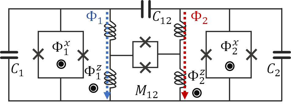
Figure 1: Circuit schematic for the non-stoquastic two qubit rf-SQUID Ozfidan et al. (2020). The two superconducting Josephson junctions are coupled both capacitively and inductively.

We present here a detailed study of how the method outlined in the previous section can be used to simulate this circuit efficiently.

The values of the fixed parameters in the above Hamiltonian are given in Table 1.

Parameter		Qubit 1		Qubit 2
$L$ (pH)		231.9		239.1
$C$ (fF)		119.5		116.4
$I$ ($\mu$A)		3.227		3.157
$C_{12}$ (fF)		132.0

Table 1: Fixed circuit parameters for the coupled rf-SQUID system. See Ref. Ozfidan et al. (2020) for more details.

The parameters not listed in Table 1 are adjustable device parameters used for initializing and performing the annealing process. To initialize the system, the coaxial fluxes, $\phi_{1}^{z}$ and $\phi_{2}^{z}$, are set to the values associated with the problem Hamiltonian. These flux values define the final state to be measured at the end of the anneal. The transverse fluxes, $\phi_{1}^{x}=\phi_{2}^{x}=\phi_{x}$, are then varied slowly, transforming the system from a single, anharmonic well at $\phi_{x}=0$ to a set of four wells at $\phi_{x}=\pi$ Lanting et al. (2014). These four wells define the four possible 2-qubit states, the lowest of which being the ground state of the final system and the solution to the problem Hamiltonian. This process is shown schematically in Fig. 2.

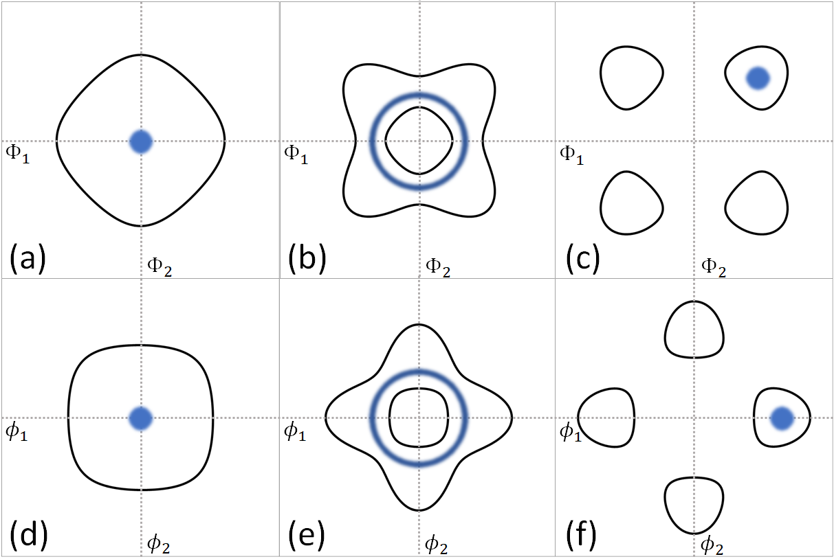
Figure 2: Schematic overview of the change in the potential energy of the two qubit circuit Hamiltonian during the annealing process. (a) Single contour of the potential energy at $\phi_{x}=0$. The dot represents the majority of the probability density of the ground state wavefunction. (b) Single contour of the potential energy at $\phi_{x}=3\pi/4$. The solid ring represents the majority of the probability density of the ground state wavefunction, which is delocalized due to the presence of a phase transition. (c) Single contour of the potential energy at $\phi_{x}=\pi$. The dot represents the majority of the probability density of the ground state wavefunction, which is in the well associated with the $|00\rangle$ qubit state. (d)-(f) Same as (a), (b), and (c) but after the normal mode transformation.

As was outlined in the previous section, we cannot work directly with Eq. (5), owing to the first order charge coupling ($\hat{Q}_{1}\hat{Q}_{2}$). Instead we transform to new coordinates,

$$\hat{q}_{1(2)}=\Bigg{(}\frac{1}{8\sqrt{\omega_{1}\omega_{2}}}\Bigg{)}^{1/2}\Big{(}\sqrt{\omega_{1}}~{}\hat{u}_{1}\mp\sqrt{\omega_{2}}~{}\hat{u}_{2}\Big{)}$$ (6)

and,

$$\hat{\phi}_{1(2)}=\Bigg{(}\frac{2}{\sqrt{\omega_{1}\omega_{2}}}\Bigg{)}^{1/2}\Big{(}\sqrt{\omega_{2}}~{}\hat{v}_{1}\mp\sqrt{\omega_{1}}~{}\hat{v}_{2}\Big{)},$$ (7)

The dimensionless operators, $\hat{u}$ and $\hat{v}$, are defined as $\hat{Q}_{i}=\sqrt{\hbar\tilde{C}_{i}\omega_{i}}~{}\hat{u}_{i}$ and $\hat{\Phi}_{i}=\sqrt{\frac{\hbar}{\tilde{C}_{i}\omega_{i}}}~{}\hat{v}_{i}+\phi_{i}^{z}$, with $\omega_{i}^{2}=1/L_{i}\tilde{C}_{i}$. This yields kinetic and potential operators of the form,

$$\hat{T}(\hat{q}_{1},\hat{q}_{2})=C_{+}~{}\hat{q}^{2}_{1}+C_{-}~{}\hat{q}^{2}_{2},$$ (8)

and,

$$\hat{V}(\hat{\phi}_{1},\hat{\phi}_{2})=L_{-}~{}\hat{\phi}^{2}_{1}+L_{+}~{}\hat{\phi}^{2}_{2}+L_{12}~{}\hat{\phi}_{1}\hat{\phi}_{2}$$

$$+E_{1}(\phi_{x})\cos\Big{[}\frac{2\pi}{\phi_{0}}\big{(}\Omega_{1}(\hat{\phi}_{1}+\hat{\phi}_{2})+\phi_{1}^{z}\big{)}\Big{]}$$

$$+E_{2}(\phi_{x})\cos\Big{[}\frac{2\pi}{\phi_{0}}\big{(}\Omega_{2}(\hat{\phi}_{1}-\hat{\phi}_{2})+\phi_{2}^{z}\big{)}\Big{]},$$ (9)

the coefficients of which are presented in Table 2.

Coefficient		Expression
$\tilde{C}_{1(2)}$		$C_{1(2)}+\frac{C_{12}C_{2(1)}}{C_{2(1)}+C_{12}}$
$C_{\pm}$		$2\hbar\sqrt{\omega_{1}\omega_{2}}\Big{(}1\mp\frac{C_{12}\sqrt{\tilde{C}_{1}\tilde{C}_{2}}}{C_{1}C_{2}+C_{12}(C_{1}+C_{2})}\Big{)}$
$L_{\pm}$		$\frac{\hbar}{16\sqrt{\omega_{1}\omega_{2}}}\Big{(}\omega_{1}^{2}+\omega_{2}^{2}\mp\frac{2M_{12}}{L_{l}L_{2}\tilde{C}_{1}\tilde{C}_{2}}\Big{)}$
$L_{12}$		$\frac{\hbar}{4\sqrt{\omega_{1}\omega_{2}}}\big{(}\omega_{1}^{2}-\omega_{2}^{2}\big{)}$
$E_{i}(\phi_{x})$		$\frac{\phi_{0}}{2\pi}I_{i}\cos\big{[}\frac{\pi}{\phi_{0}}\phi_{x}\big{]}$
$\Omega_{i}$		$\Big{(}\frac{\hbar}{8\tilde{C}_{i}\sqrt{\omega_{1}\omega_{2}}}\Big{)}^{1/2}$

Table 2: Coefficients for the two qubit rf-SQUID circuit normal mode Hamiltonian.

Results.— We simulate the circuit outlined in the previous section, Eq. (4), by employing off-diagonal expansion QMC (ODE QMC) Albash et al. (2017); Hen (2018); Gupta et al. (2020). Using this, we can compute the thermal average of observable quantities by $\langle\hat{A}\rangle=\textsf{Tr}[\hat{A}e^{-\beta\hat{H}}]/\textsf{Tr}[e^{-\beta\hat{H}}]$, where $\beta=1/kT$ (here we chose $T=12m$K to reflect actual device temperatures). The quantity of interest for superconducting flux qubits and AQC is the persistent current, $\hat{I}_{1(2)}^{z}$, the expectation value of which can be expressed as,

$$\langle\hat{I}_{1(2)}^{z}\rangle=-\Bigg{\langle}\frac{\partial\hat{H}}{\partial\phi_{1(2)}^{z}}\Bigg{\rangle}=$$

$$\frac{1}{L_{1(2)}}\Big{(}\langle\hat{\Phi}_{1(2)}\rangle-\phi_{1(2)}^{z}\Big{)}+\frac{M_{12}}{L_{1}L_{1}}\Big{(}\langle\hat{\Phi}_{2(1)}\rangle-\phi_{2(1)}^{z}\Big{)}.$$ (10)

The above constitutes the “qubit” in superconducting flux qubit device, since the quantized current (or more appropriately, the direction of the quantized current) is what maps to the spin up (or down) in the qubit model, analogous to the eigenstates of the Pauli-z operator Kjaergaard et al. (2019). In other words, this is the quantity that is measured by the hardware, and a clockwise (or counterclockwise) current yields a positive (or negative) current measurement, which is interpreted as a qubit state of $|0\rangle$ (or $|1\rangle$).

Our algorithm has only one extraneous parameter, the grid spacing $\Delta$. It is important to make sure that in the limit $\Delta\rightarrow 0$, the discretized model approaches the continuous Hamiltonian. This is presented in Fig. 3 which shows the relative error for $\langle\hat{I}_{1}^{z}\rangle$ as a function of $\Delta$ computed using exact diagonalization, confirming our expectations that our simulations recover the results of the continuous model for small enough $\Delta$.

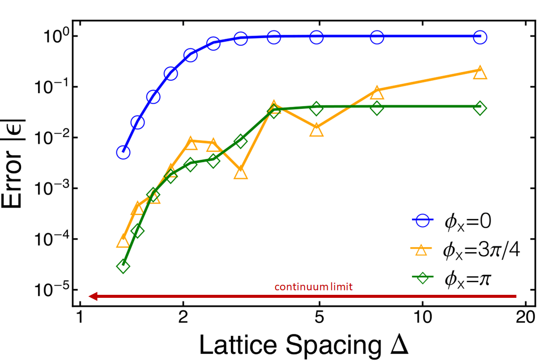
Figure 3: Magnitude of the relative error of the persistent current as a function of the convergence parameter $\Delta$. The current was computed using $\phi_{1}^{z}=0.1~{}m\phi_{0}$ and $\phi_{2}^{z}=0.9~{}m\phi_{0}$ at three different points in the anneal.

To demonstrate that we can, in fact, simulate the circuit, we computed four separate anneals for four sample problem Hamiltonians, each corresponding to the four possible 2-qubit readouts—$~{}|00\rangle,|01\rangle,|10\rangle$, and $|11\rangle$. We dictate which of the final states we desire by setting the coaxial fluxes, $\phi_{1}^{z}$ and $\phi_{2}^{z}$, to either positive or negative values depending on the desired state. The magnitude of these chosen values would come from the problem Hamiltonian one would be attempting to solve using AQC. For the purposes here, they were chosen arbitrarily to showcase the versatility of our technique. This is illustrated in Fig. 4.

We can relate the change in $\hat{I}_{z}$ shown in Fig. 4 back to the schematic shown in Fig. 2 by noting again that each of the four qubits states correspond to a well in one of the four Cartesian quadrants of the $(\hat{\Phi}_{1},\hat{\Phi}_{2})$ plane. These qubit states also correspond to a set of measurements of the sign of $I_{1}^{z}$ and $I_{2}^{z}$. For example, setting both $\phi_{1}^{z}$ and $\phi_{2}^{z}$ to positive values results in the well in the $(+,+)$ quadrant being the lowest in energy, as well as $I_{1}^{z}$ and $I_{2}^{z}$ both have a positive sign, as in Fig. 4(a). Expressed differently, Fig. 4 illustrates that the sign of the current readout corresponds to the quadrant in which the lowest energy well is located.

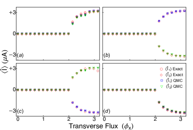
Figure 4: Persistent current calculated for both exact diagonalization and ODE QMC at various $\phi_{x}$ points throughout the annealing process. (a) Anneal for the $|00\rangle$ qubit output. $\phi_{1}^{z}=0.1~{}\text{m}\phi_{0}$ and $\phi_{2}^{z}=0.9~{}\text{m}\phi_{0}$ were used as the problem Hamiltonian values. (b) $|01\rangle$, $\phi_{1}^{z}=0.5$ and $\phi_{2}^{z}=-0.5$ (c) $|10\rangle$, $\phi_{1}^{z}=-0.4$ and $\phi_{2}^{z}=0.25$ (d) $|11\rangle$, $\phi_{1}^{z}=-0.25$ and $\phi_{2}^{z}=-0.25$.

It is interesting to note that the qubit representations of the circuits simulated above are virtually unsimulable by QMC due to the severe sign problem caused by the NStoq terms that arise from the reduction of the circuit Gupta and Hen (2020); Ozfidan et al. (2020).
Conclusions.— In this study, we devised a prescription to make seemingly NStoq superconducting flux circuits amendable to scalable, efficient QMC techniques. The importance of our work lies mainly in its implications for approximating superconducting circuits as qubit models, and what information about the circuit can be gleaned from simulations of the model. Our results stand in stark contrast with recent and ongoing efforts to construct circuits of this type Ozfidan et al. (2020). If indeed superconducting flux circuits—even those circuits whose qubit representations are NStoq—are efficiently simulable, then the implications are that flux circuits cannot generate genuine non-stoquastic dynamics, which is an important ingredient for both AQC universality and quantum supremacy.

While the focus of our work was one specific superconducting flux qubit device, we note that our analysis equally applies for any “traditional” qubit circuit and that we expect to maintain QMC scaling, poly($n$), irrespective of system size. Our conclusions are predicated on the grid spacing being constant as a function of system size, which is expected since the grid spacing is proportional to the scale of the distance between wells in the flux hyperspace, which are relatively constant with respect to system size.

The method laid out here is predicated on the limitation that the charge part of the Hamiltonian can be made Cartesian via some sort of transformation. Therefore, an important question that arises from our work is: What modifications to the Hamiltonians of superconducting flux circuits can be made for these systems to truly exhibit non-stoquasticity at the circuit level? One obvious choice is to introduce an external vector potential; however, this will only results in an offset charge operator, which can, most likely, be gauged away via a coordinate transformation. Currently, the most likely candidate to produce a truly NStoq circuit is a Hamiltonian that couples the charge and flux operators. This is exactly what is being explored by the bifluxon qubit system Kalashnikov et al. (2020). We conclude that AQC would benefit greatly from more effort being put into the study of systems of this type in order to achieve this long sought after goal—mainly, a truly unsimulable circuit Hamiltonian.

An interesting conjecture that follows from our results is that every NStoq (and thus non-simulable) spin model is a low-energy approximation of a higher-dimensional Stoq model. If this is the case and an efficient construction of such higher-dimensional models exists, that might be a path towards resolving the infamous QMC sign problem Marvian et al. (2019); Gupta and Hen (2020).

Acknowledgments.—We would like to extend a special thanks to David Ferguson for many insightful discussions. We would also like to thank Tameem Albash, Elizabeth Crosson, Mostafa Khezri, Harel Kol-Namer and Milad Marvian for valuable comments. Computation for the work described here was supported by the University of Southern California’s Center for High-Performance Computing (http://hpcc.usc.edu). The research is based upon work (partially) supported by the Office of the Director of National Intelligence (ODNI), Intelligence Advanced Research Projects Activity (IARPA), via the U.S. Army Research Office contract W911NF-17-C-0050. This material is based on research sponsored by the Air Force Research laboratory under agreement number FA8750-18-1-0044. Special thanks to the U.S.-Israel Binational Science Foundation (Grant No. 2016224) and the Israel Science Foundation (Grant No. 227/15). The U.S. Government is authorized to reproduce and distribute reprints for Governmental purposes notwithstanding any copyright notation thereon. The views and conclusions contained herein are those of the authors and should not be interpreted as necessarily representing the official policies or endorsements, either expressed or implied, of the ODNI, IARPA, or the U.S. Government.

Appendix A QMC simulation of superconducting flux circuits: technical details

We simulate the flux circuits using the permutation matrix representation (PMR) QMC technique introduced and described in Refs. Albash et al. (2017); Hen (2018); Gupta et al. (2020). The method is based on the off-diagonal expansion of the quantum partition function Albash et al. (2017); Hen (2018) wherein the Hamiltonian is cast in the form,

$$H=\sum_{j=0}^{M}D_{j}P_{j}\,,$$ (11)

with the matrices $D_{j}$ and $P_{j}$ represented in the computational basis, $\{|z\rangle\}$. For $j=0$, $P_{j}$ is the identity, $P_{0}=\mathbb{1}$, and for $j>0$, $P_{j}$ are permutation operators with no fixed points—i.e., $P_{j>0}$ is purely off-diagonal. Conversely, $D_{j}$ is purely diagonal. This formulation allows us to write the canonical partition function as the sum

$$Z=\sum_{\{z\}}\sum_{q=0}^{\infty}\sum_{\{S_{{\bf{i}}_{q}}\}}D_{(z,S_{{\bf{i}}_{q}})}\langle z|S_{{\bf{i}}_{q}}|z\rangle{{e}}^{-\beta[E_{z_{0}},\ldots,E_{z_{q}}]}\,,$$ (12)

where $\{S_{{\bf{i}}_{q}}\}$ is the set of all (unevaluated) products $P_{i_{q}}\ldots P_{i_{2}}P_{i_{1}}$ of size $q$, ${\bf i}_{q}=(i_{1},\ldots,i_{q})$ is a multiple index where each individual index $i_{j}$ (with $j=1\ldots q$) ranges from $1$ to $M$, and the term $e^{-\beta[E_{z_{0}},\ldots,E_{z_{q}}]}$ is the divided differences of the exponential function over the multiset of classical energies $[E_{z_{0}},\ldots E_{z_{q}}]$ Whittaker and Robinson (1967); de Boor (2005). The energies $\left\{E_{z_{i}}=\langle z_{i}|H_{\text{c}}|z_{i}\rangle\right\}$ are the classical energies of the states $|z_{0}\rangle,\ldots,|z_{q}\rangle$, obtained from the action of the ordered $P_{j}$ operators in the sequence, $S_{{\bf{i}}_{q}}$, acting on $|z_{0}\rangle$ through $|z_{q}\rangle$. We also denote,

$$D_{(z,S_{{\bf{i}}_{q}})}=\prod_{j=1}^{q}d^{(i_{j})}_{z_{j}}\,,$$ (13)

where $d^{(i_{j})}_{z_{j}}$ is the “hopping strength” of $P_{i_{j}}$ with respect to $|z_{j}\rangle$, given explicitly by,

$$d^{(i_{j})}_{z_{j}}=\langle z_{j}|D_{i_{j}}|z_{j}\rangle\,.$$ (14)

For further details we refer the reader to Ref. Gupta et al. (2020).

To simulate flux circuit Hamiltonians with PMR we first cast the discretized Hamiltonian, Eq. (4), in the form of Eq. (11), by regrouping terms. Specifically, we rewrite the equation as

$$H=\sum_{j=-M}^{M}D_{j}P_{j}\,.$$ (15)

For $j=0$, $P_{0}=\sum_{I}|I\rangle\langle I|$, which is the identity (as expected), and $D_{0}=\sum_{I}\Big{(}V_{I}+\frac{2\mu\hbar^{2}}{\Delta^{2}}\Big{)}|I\rangle\langle I|$ , where $\mu=\sum_{k=1}^{n}\mu_{k}$. For $j\neq 0$, the permutation operators are then given by,

$$P_{\pm j}=\sum_{I}|I_{j}^{(\pm)}\rangle\langle I|\,.$$ (16)

In matrix form, $P_{j}$ and $P_{-j}$ are zero everywhere except for the first upper and lower diagonal respectively being unity. These two operators have the property, $P_{j}P_{-j}=\mathbb{1}$. The corresponding diagonal operators are $D_{j}=\sum_{I}\Big{(}-\frac{\mu_{j}\hbar^{2}}{\Delta^{2}}\Big{)}|I\rangle\langle I|$ for all $j$.

The QMC configuration for this model is given by ${\cal C}=\{|I\rangle,S_{{\bf{i}}_{q}}\}$—i.e., a basis state $|I\rangle$ and a sequence of permutation operators $S_{{\bf{i}}_{q}}=P_{i_{q}}\cdots P_{i_{2}}P_{i_{1}}$ that evaluate to the identity operation. The initial configuration ${\cal C}_{0}$ of the simulation consists of a random basis state $|I_{0}\rangle$ and the empty sequence $S_{i_{0}}$. The weight of this initial configuration is thus

$$W_{{\cal C}_{0}}=D_{(I_{0},S_{0})}e^{-\beta[E_{I_{0}}]}=e^{-\beta E_{I_{0}}}$$ (17)

where $E_{I_{0}}$ is the classical energy corresponding to $|I_{0}\rangle$.

We next review the QMC updates used in our simulations.
Classical Move (short-step): In this move we shift the basis state by one grid spacing in a randomly chosen direction $|I\rangle\rightarrow|I_{k}^{(\pm)}\rangle$ for some randomly chosen direction $k$, leaving the permutation operator sequence $S_{{\bf{i}}_{q}}$ unchanged. If we let ${\cal C}$ be the configuration before the move and ${\cal C^{\prime}}$ the configuration after the move, then we can express the acceptance probability for a classical move as

$$p=\min\left(1,\frac{W_{{\cal C}^{\prime}}}{W_{{\cal C}}}\right)=\min\left(1,\frac{{{e}}^{-\beta[E_{{\cal C}^{\prime}}]}}{{{e}}^{-\beta[E_{{\cal C}}]}}\right)\,,$$ (18)

where ${{e}}^{-\beta[E_{{\cal C}}]}$ is a shorthand for ${{e}}^{-\beta[E_{z_{0}},E_{z_{1}},\ldots,E_{z_{q}}]}$ of configuration ${\cal C}$ (and ${\cal C}^{\prime}$).

Classical Move (long-step): For the long-step classical move we follow the same procedure except instead of a step size of one, we use a step size $M$. We take $M$ to be proportional to $D/\Delta$ where $D$ is the distance between minima of the potential wells. This can be done because we know a priori that the potential energy surface has a finite number of well separated minima. These larger steps help eliminate the chance of being stuck (for a long time) in a local minimum, resulting in dramatically reduced equilibration time. Again, we take ${\cal C}$ to be the configuration before the move and ${\cal C^{\prime}}$ to be the configuration after, allowing for the same acceptance probability seen in Eq. (18).

Block-swap Move: A block swap update involves the change of both the basis state and sequence of permutation operator $S_{{\bf{i}}_{q}}$. In this move a random position $j$ in the product $S_{{\bf{i}}_{q}}$ is picked, and the product is split into two (non-empty) sub-sequences, $S_{{\bf{i}}_{q}}=S_{1}S_{2}$, with $S_{1}=P_{i_{q}}\cdots P_{i_{j+1}}$ and $S_{2}=P_{i_{j}}\cdots P_{i_{1}}$. The state $|I^{\prime}\rangle$ at position $j$ in the product can be mapped back to the current state, $|I\rangle$, by $\langle I^{\prime}|=\langle I|S_{1}=\langle I|P_{i_{1}}\dots P_{i_{j}}$, where $|I\rangle$ and $|I^{\prime}\rangle$ have energies $E_{I}$ and $E_{I^{\prime}}$, respectively. This gives a new block-swapped configuration as ${\cal C}^{\prime}=\{|I^{\prime}\rangle,S_{2}S_{1}\}$ and a weight that is proportional to $e^{-\beta[E_{{\cal C}^{\prime}}]}$ where the multiset $E_{{\cal C}^{\prime}}=E_{{\cal C}}+\{E_{I^{\prime}}\}-\{E_{I}\}$. Lastly, we can again express the acceptance probability in the same manner as in Eq. (18), using the aforementioned $E_{{\cal C}^{\prime}}$.
Cycle completion Move: All moves presented thus far have left $q$ unchanged in that the number of elements in the sequence has remained constant. Cycle completion moves, on the other hand, change the value of $q$. In this type of move we randomly pick a point, $j\in[0,q]$, in the sequence. This point defines a subsequence of the form $P_{0}P_{0}$ or $P_{i_{j}}P_{i_{j+1}}$, with $P_{0}$ and $P_{q+1}$ corresponding to the identity. The new configuration $\mathcal{C}^{\prime}$ is then defined by replacing the identified subsequence by an equivalent subsequence of length at most two. The two subsequence $P_{i_{j}}P_{i_{k}}$ and $P_{i_{j}}^{\prime}P_{i_{k}}^{\prime}$ are equivalent if $(P_{i_{j}}P_{i_{k}}).{(P_{i_{j}}^{\prime}P_{i_{k}}^{\prime})}^{-1}=\mathbb{1}$. Because we can interpret $P_{0}^{-1}=P_{0}=P_{j}P_{j}^{-1}$ (for any arbitrary index $j$) and so on, the cycle completion move can grow and shrink the sequence. The acceptance probability is the same before (see Eq. (18)).

The last step in QMC is to take a measurement of some observable. Below we briefly describe the diagonal measurement in our QMC model.
Diagonal measurement: We know that any diagonal operator, $\Lambda$, obeys the eignevalue equation $\Lambda|I\rangle=\lambda_{I}|I\rangle$, where $\lambda_{I}$ is the eigenvalue of $\Lambda$ for eigenstate $|I\rangle$. We also know that that for any configurationm ${\cal C}=\{|I\rangle,S_{{\bf{i}}_{q}}\}$, there is a contribution to the thermal average $\langle\Lambda\rangle$ given by $\langle I|\Lambda S_{{\bf{i}}_{q}}|I\rangle=\lambda_{I}\langle I|S_{{\bf{i}}_{q}}|I\rangle$, assuming $\Lambda$ is Hermitian. All of this allows for the simple measurement of $\langle\hat{\Phi}\rangle$, since the basis states, $|I\rangle=|i_{1},...,i_{n}\rangle$, are approximate eigenstates of, $\hat{\Phi}_{k}$, with eigenvalues $\lambda=i_{k}\Delta$. This is useful because the quantity of interest is $\hat{I}^{z}$, which is a weighted sum of $\hat{\Phi}$’s—i.e., $\hat{I}^{z}$ is also diagonal.

References

- Albash and Lidar (2018) T. Albash and D. A. Lidar, Rev. Mod. Phys. 90, 015002 (2018).
- Biamonte and Love (2008) J. D. Biamonte and P. J. Love, Phys. Rev. A 78, 012352 (2008).
- Aharonov et al. (2007) D. Aharonov, W. van Dam, J. Kempe, Z. Landau, S. Lloyd, and O. Regev, SIAM J. Comput. 37, 166 (2007).
- Bravyi and Terhal (2009) S. Bravyi and B. Terhal, SIAM Journal on Computing, SIAM Journal on Computing 39, 1462 (2009).
- Marvian et al. (2019) M. Marvian, D. A. Lidar, and I. Hen, Nature Communications 10, 1571 (2019).
- Klassen and Terhal (2019) J. Klassen and B. M. Terhal, Quantum 3, 139 (2019).
- Klassen et al. (2019) J. Klassen, M. Marvian, S. Piddock, M. Ioannou, I. Hen, and B. Terhal, arXiv e-prints , arXiv:1906.08800 (2019), arXiv:1906.08800 [quant-ph] .
- Gupta and Hen (2020) L. Gupta and I. Hen, Advanced Quantum Technologies 3, 1900108 (2020).
- Crosson et al. (2020) E. Crosson, T. Albash, I. Hen, and A. P. Young, “De-signing hamiltonians for quantum adiabatic optimization,” (2020), arXiv:2004.07681 [quant-ph] .
- Troyer and Wiese (2005) M. Troyer and U.-J. Wiese, Phys. Rev. Lett. 94, 170201 (2005).
- Crosson et al. (2014) E. Crosson, E. Farhi, C. Yen-Yu Lin, H.-H. Lin, and P. Shor, ArXiv e-prints (2014), arXiv:1401.7320 [quant-ph] .
- Nishimori and Takada (2017) H. Nishimori and K. Takada, Frontiers in ICT 4, 2 (2017).
- Vinci and Lidar (2017) W. Vinci and D. A. Lidar, npj Quantum Information 3, 38 (2017).
- Hormozi et al. (2017) L. Hormozi, E. W. Brown, G. Carleo, and M. Troyer, Phys. Rev. B 95, 184416 (2017).
- Albash (2019) T. Albash, Phys. Rev. A 99, 042334 (2019).
- Susa et al. (2017) Y. Susa, J. F. Jadebeck, and H. Nishimori, Phys. Rev. A 95, 042321 (2017).
- Durkin (2019) G. A. Durkin, Phys. Rev. A 99, 032315 (2019).
- Kjaergaard et al. (2020) M. Kjaergaard, M. E. Schwartz, J. Braumüller, P. Krantz, J. I.-J. Wang, S. Gustavsson, and W. D. Oliver, Annual Review of Condensed Matter Physics 11, 369 (2020), https://doi.org/10.1146/annurev-conmatphys-031119-050605 .
- Ozfidan et al. (2020) I. Ozfidan, C. Deng, A. Smirnov, T. Lanting, R. Harris, L. Swenson, J. Whittaker, F. Altomare, M. Babcock, C. Baron, A. Berkley, K. Boothby, H. Christiani, P. Bunyk, C. Enderud, B. Evert, M. Hager, A. Hajda, J. Hilton, S. Huang, E. Hoskinson, M. Johnson, K. Jooya, E. Ladizinsky, N. Ladizinsky, R. Li, A. MacDonald, D. Marsden, G. Marsden, T. Medina, R. Molavi, R. Neufeld, M. Nissen, M. Norouzpour, T. Oh, I. Pavlov, I. Perminov, G. Poulin-Lamarre, M. Reis, T. Prescott, C. Rich, Y. Sato, G. Sterling, N. Tsai, M. Volkmann, W. Wilkinson, J. Yao, and M. Amin, Phys. Rev. Applied 13, 034037 (2020).
- Bravyi et al. (2008) S. Bravyi, D. P. DiVincenzo, R. I. Oliveira, and B. M. Terhal, Quant. Inf. Comp. 8, 0361 (2008).
- Burkard et al. (2004) G. Burkard, R. H. Koch, and D. P. DiVincenzo, Phys. Rev. B 69, 064503 (2004).
- Note (1) An independent study making similar assertions that has very recently been posted on the arXiv Ciani and Terhal (2020). However, the focus and methods by which the resolution of the off-diagonal matrix elements in the kinetic energy matrix is achieved are quite different.
- Vool and Devoret (2017) U. Vool and M. Devoret, International Journal of Circuit Theory and Applications 45, 897 (2017).
- Landau and Binder (2005) D. P. Landau and K. Binder, A guide to Monte Carlo Methods in Statistical Physics, 2nd Ed. (Cambridge University Press, New York, USA, 2005).
- Newman and Barkema (1999) M. E. J. Newman and G. T. Barkema, Monte Carlo Methods in Statistical Physics (Oxford University Press Inc., New York, USA, 1999).
- Note (2) Of course, not much can be said about the scaling of the QMC equilibration time; even the most carefully chosen basis may still yield painfully long computation times due to the system being difficult to equilibrate, e.g., it has a highly degenerate ground state. This is true regardless of system size, and is not unique to QMC—i.e., quantum annealers may similarly take exponential times to equilibrate.
- Colbert and Miller (1992) D. T. Colbert and W. H. Miller, The Journal of chemical physics 96, 1982 (1992).
- Littlejohn et al. (2002) R. G. Littlejohn, M. Cargo, T. Carrington Jr, K. A. Mitchell, and B. Poirier, The Journal of chemical physics 116, 8691 (2002).
- Halverson and Poirier (2015) T. Halverson and B. Poirier, Chemical Physics Letters 624, 37 (2015).
- Halverson et al. (2018) T. Halverson, D. Iouchtchenko, and P.-N. Roy, The Journal of chemical physics 148, 074112 (2018).
- Harris et al. (2010) R. Harris, J. Johansson, A. Berkley, M. Johnson, T. Lanting, S. Han, P. Bunyk, E. Ladizinsky, T. Oh, I. Perminov, et al., Physical Review B 81, 134510 (2010).
- Krantz et al. (2019) P. Krantz, M. Kjaergaard, F. Yan, T. P. Orlando, S. Gustavsson, and W. D. Oliver, Applied Physics Reviews 6, 021318 (2019).
- Fagaly (2006) R. Fagaly, Review of scientific instruments 77, 101101 (2006).
- Lanting et al. (2014) T. Lanting, A. J. Przybysz, A. Y. Smirnov, F. M. Spedalieri, M. H. Amin, A. J. Berkley, R. Harris, F. Altomare, S. Boixo, P. Bunyk, N. Dickson, C. Enderud, J. P. Hilton, E. Hoskinson, M. W. Johnson, E. Ladizinsky, N. Ladizinsky, R. Neufeld, T. Oh, I. Perminov, C. Rich, M. C. Thom, E. Tolkacheva, S. Uchaikin, A. B. Wilson, and G. Rose, Phys. Rev. X 4, 021041 (2014).
- Albash et al. (2017) T. Albash, G. Wagenbreth, and I. Hen, Phys. Rev. E 96, 063309 (2017).
- Hen (2018) I. Hen, Journal of Statistical Mechanics: Theory and Experiment 2018, 053102 (2018).
- Gupta et al. (2020) L. Gupta, T. Albash, and I. Hen, Journal of Statistical Mechanics: Theory and Experiment 2020, 073105 (2020).
- Kjaergaard et al. (2019) M. Kjaergaard, M. E. Schwartz, J. Braumüller, P. Krantz, J. I.-J. Wang, S. Gustavsson, and W. D. Oliver, Annual Review of Condensed Matter Physics 11 (2019).
- Kalashnikov et al. (2020) K. Kalashnikov, W. T. Hsieh, W. Zhang, W.-S. Lu, P. Kamenov, A. Di Paolo, A. Blais, M. E. Gershenson, and M. Bell, PRX Quantum 1, 010307 (2020).
- Ciani and Terhal (2020) A. Ciani and B. M. Terhal, arXiv e-prints , arXiv:2011.01109 (2020), arXiv:2011.01109 [quant-ph] .
- Whittaker and Robinson (1967) E. T. Whittaker and G. Robinson, in The Calculus of Observations: A Treatise on Numerical Mathematics (New York: Dover, New York, 1967).
- de Boor (2005) C. de Boor, Surveys in Approximation Theory 1, 46 (2005).