Non-minimally Coupled Einstein-Gauss-Bonnet Gravity with Massless Gravitons: The Constant-roll Case

Abstract

In this letter we study the behavior of non-minimally coupled Einstein-Gauss-Bonnet gravity theories with the constant-roll condition. Recalling the results of the striking GW170817 event, we demand that the velocity of the gravitational waves is equated to unity in natural units, meaning that $c_{T}^{2}=1$. This is a powerful restriction since it leads to a decrease in the degrees of freedom and subsequently reveals a connection between the scalar functions of the theory which presumably have different origins. In this framework, we shall assume that a scalar potential is present and can be extracted easily from the equations of motion by simply designating the scalar coupling functions. Obviously, a different approach is feasible but such choice will prove to be extremely convenient. Afterwards, we impose certain approximations in order to facilitate our study. Each assumption is capable of producing different phenomenology so a summary of all the possible configurations for Hubble’s parameter, its derivative and the scalar potential along with the corresponding assumptions are present at the end of the paper. We show that compatibility under the constant-roll assumption can be achieved for a variety of model functions and different approaches, although one must always be aware of the imposed approximations since the possibility of a model producing viable results while simultaneously violating even a single approximation exists. Finally, in the end, a new formalism which leads to a plethora of convenient coupling functions according to the readers choice is presented. Utilizing such formalism may lead to new cases for coupling functions which have not been used yet, but are in fact able of producing viable phenomenology for the inflationary era.

I Introduction

In the literature, there exists a plethora of non minimally coupled gravity theories which are capable of producing viable results. Such a theory is also the Einstein-Gauss-Bonnet theory Hwang:2005hb ; Nojiri:2006je ; Cognola:2006sp ; Nojiri:2005vv ; Nojiri:2005jg ; Satoh:2007gn ; Bamba:2014zoa ; Yi:2018gse ; Guo:2009uk ; Guo:2010jr ; Jiang:2013gza ; Kanti:2015pda ; vandeBruck:2017voa ; Kanti:1998jd ; Pozdeeva:2020apf ; Fomin:2020hfh ; DeLaurentis:2015fea ; Chervon:2019sey ; Nozari:2017rta ; Odintsov:2018zhw ; Kawai:1998ab ; Yi:2018dhl ; vandeBruck:2016xvt ; Kleihaus:2019rbg ; Bakopoulos:2019tvc ; Maeda:2011zn ; Bakopoulos:2020dfg ; Ai:2020peo ; Odintsov:2019clh ; Oikonomou:2020oil ; Odintsov:2020xji ; Oikonomou:2020sij ; Odintsov:2020zkl ; Odintsov:2020sqy ; Odintsov:2020mkz ; Easther:1996yd ; Antoniadis:1993jc ; Antoniadis:1990uu ; Kanti:1995vq ; Kanti:1997br , once certain constraints are imposed. In order to achieve viability, it is mandatory to equate the velocity of the gravitational waves with the speed of light, as stated by the GW170817 event GBM:2017lvd . This case has been studied thoroughly in Odintsov:2019clh ; Oikonomou:2020oil ; Odintsov:2020xji ; Odintsov:2020zkl ; Odintsov:2020sqy ; Oikonomou:2020sij ; Odintsov:2020mkz assuming a slow-roll evolution. In the present paper, we shall follow a physically different approach which, as it turns out, can also lead to viable phenomenology. Assuming a constant-roll evolution for the scalar field, which shall be implemented in the present paper, the behavior of the scalar field $\phi$ is completely different. Now, the rate of change of the scalar field is decided by a single parameter, the constant-roll parameter. This is also the decisive factor in the resulting values of the observational quantities of inflation since for example the spectral index of the primordial curvature perturbations is strongly affected by this particular parameter, hence the reason why the constant-roll assumption is convenient. In this paper, we shall develop and present the framework of constant-roll Einstein-Gauss-Bonnet gravity in detail. After specifying the gravitational action and deriving the equations of motion, constraints on the velocity of the gravitational waves are imposed in order to achieve a viable phenomenology compatible with the GW170817. Combining this restriction and the constant-roll assumption, a functional relation for scalar field is produced. Then, the slow-varying parameters such as the slow-roll indices, which play a significant role in our study, are introduced. In the following sections, we present a variety of designations for the scalar coupling functions following functional assumptions for the equations of motion. In each case, the corresponding scalar potential which is present in this framework, is derived directly from the equations of motion and then we compare the results of each model and study the behavior of the system under changes in the values of the free parameters. Finally, we discuss and present in detail all the possible approximations of the equations of motion and in the appendix, we include a pedagogical new formalism which materializes various approximations in non-minimal Einstein-Gauss-Bonnet gravity, and we make it available to the interested reader.

At this point, it is also worth mentioning that in the present paper, the cosmological background will be assumed to be that of a flat Friedman-Robertson-Walker metric, with the corresponding line element being,

$$\centering ds^{2}=-dt^{2}+\sum_{i=1}^{3}{(dx^{i})^{2}},\,\@add@centering$$ (1)

where $a(t)$ denotes the scale factor.

II Essential Features of Constant-Roll Inflation of non-minimally Coupled Einstein-Gauss-Bonnet Gravity

In this section we shall present the formalism of inflationary dynamics in the context of non-minimally coupled Einstein-Gauss-Bonnet. The corresponding gravitational action is assumed to be equal to,

$$\centering S=\int{d^{4}x\sqrt{-g}\left(\frac{h(\phi)R}{2\kappa^{2}}-\frac{1}{2}\omega g^{\mu\nu}\partial_{\mu}\phi\partial_{\nu}\phi-V(\phi)-\xi(\phi)\mathcal{G}\right)},\,\@add@centering$$ (2)

where $g$ is the determinant of the metric tensor $g_{\mu\nu}$ specified previously in the line element, $R$ denotes the Ricci scalar, $h(\phi)$ is a dimensionless scalar function coupled to the Ricci scalar and $V(\phi)$ signifies the scalar potential of the scalar field and finally, the term $\xi(\phi)\mathcal{G}$ refers to the string corrections with $\mathcal{G}$ being the Gauss-Bonnet invariant and $\xi(\phi)$ the Gauss-Bonnet coupling scalar function. In particular, the Gauss-Bonnet invariant is defined as $\mathcal{G}=R^{2}-4R_{\alpha\beta}R^{\alpha\beta}+R_{\alpha\beta\gamma\delta}R^{\alpha\beta\gamma\delta}$ with $R_{\alpha\beta}$ and $R_{\alpha\beta\gamma\delta}$ being the Ricci and Riemann tensor respectively and due to the form of the line element, they are simplified to the expressions $\mathcal{G}=24H^{2}(\dot{H}+H^{2})$ and $R=12H^{2}+6\dot{H}$ where $H$ denotes Hubble’s parameter defined as $H=\frac{\dot{a}}{a}$ and the “dot” as usual implies differentiation with respect to the cosmic time. Furthermore, by assuming the scalar field $\phi$ is homogeneous, meaning only time dependent, then the kinetic term is also simplified to the form $-\frac{1}{2}\omega\dot{\phi}^{2}$. Finally, we mention that in the following results, we shall assume a canonical kinetic term which in turn implies that $\omega=1$, but we shall keep it as it is in order to have the phantom or non-canonical (but nevertheless constant) case available for the reader.

Implementing the variation principle with respect to the metric tensor and the scalar field in Eq. (2) generates the field equations of gravity and the continuity equation of the scalar field. By splitting the field equations in time and space components, the gravitational equations of motion are then derived which read,

$$\centering\frac{3hH^{2}}{\kappa^{2}}=\frac{1}{2}\omega\dot{\phi}^{2}+V-\frac{3H\dot{h}}{\kappa^{2}}+24\dot{\xi}H^{3},\,\@add@centering$$ (3)

$$\centering-\frac{2h\dot{H}}{\kappa^{2}}=\omega\dot{\phi}^{2}-\frac{H\dot{h}}{\kappa^{2}}-16\dot{\xi}H\dot{H}+\frac{h^{\prime\prime}\dot{\phi}^{2}+h^{\prime}\ddot{\phi}}{\kappa^{2}}-8H^{2}(\ddot{\xi}-H\dot{\xi}),\,\@add@centering$$ (4)

$$\centering\omega(\ddot{\phi}+3H\dot{\phi})+V^{\prime}-\frac{Rh^{\prime}}{2\kappa^{2}}+24\xi^{\prime}H^{2}(\dot{H}+H^{2})=0,\,\@add@centering$$ (5)

where with “prime”at this instance, we denote differentiation with respect to the scalar field. This system of equations contains all the available information of the inflationary era, but unfortunately it is very intricate and cannot be solved analytically. One may proceed only by making certain approximations which must hold true in order for the model to be rendered viable. Furthermore, in order to be called viable, the model obviously must not be at variance with the observations. Recent observations such as the striking GW170817 event have made it abundantly clear that the tensor perturbations on the metric propagate with a velocity equal to that of light’s, and therefore each model of modified gravity stating otherwise must be discarded, no matter the mathematical beauty it may involve. The modified Einstein-Gauss-Bonnet gravity is very promising since even though it generates a formula for the velocity of the gravitational waves which at first site seems to deviate from the speed of light, but it can be carefully modified in order to “survive” the test of GW170817. In particular, the expression for the velocity in natural units, where $c=1$, is,

$$\centering c_{T}^{2}=1-\frac{Q_{f}}{2Q_{t}},\,\@add@centering$$ (6)

where $Q_{f}$ and $Q_{t}$ are auxiliary functions defined as $Q_{f}=16(\ddot{\xi}-H\dot{\xi})$ and $Q_{t}=\frac{h}{\kappa^{2}}-8\dot{\xi}H$. Thus, the theory can predict velocity for the gravitational waves equal to the speed of light by equating the numerator of the second term to zero, or in other words $\ddot{\xi}=H\dot{\xi}$. This relation also simplifies the second equation of motion (4). Upon solving this ordinary differential equation, one finds the expression for the derivative of the Gauss-Bonnet coupling function. This method has been studied previously in . However, there exists a different method which seems to reveal deeper connections between the functions of the scalar field. Since the differential operator with respect to time can be replaced with one depending on the scalar field, i.e. $\frac{d}{dt}=\dot{\phi}\frac{d}{d\phi}$, then the differential equations can be rewritten as,

$$\centering\xi^{\prime\prime}\dot{\phi}^{2}+\xi^{\prime}\ddot{\phi}=H\xi^{\prime}\dot{\phi}.\,\@add@centering$$ (7)

From this equation, a deeper connection can be extracted by two different assumptions. Assuming that the slow-roll approximation holds, then $\ddot{\phi}\ll H\dot{\phi}$, thus the term $\xi^{\prime}\ddot{\phi}$ is negligible. This method has been studied thoroughly both in the minimally and non-minimally coupled case, see Odintsov:2020sqy and Odintsov:2020xji respectively. An alternative approach is to assume a constant-roll condition, which is also the one we shall implement. Letting $\ddot{\phi}=\beta H\dot{\phi}$ where $\beta$ is the constant-roll parameter, then the previous equation can be solved exactly. The resulting expression is shown below,

$$\centering\dot{\phi}=H(1-\beta)\frac{\xi^{\prime}}{\xi^{\prime\prime}},\,\@add@centering$$ (8)

where it was obviously assumed that $\dot{\phi}$ is nonzero. This in turn implies that $\beta\neq 1$ and as we shall see, this prohibition states the slow-roll indices do not drop to zero simultaneously, however their values could be small. In addition, in order to simplify the equations of motion, we shall assume that the slow-roll approximations hold true. However, the value of $\beta$ will not be assumed by definition to be small and will be examined during the fine tuning of a model. Hence, we demand that,

$$\centering\dot{H}\@add@centering \ll H^{2}, \frac{1}{2}\omega\dot{\phi} \ll V,\,$$ (9)

during the first horizon crossing, or the initial stage of inflation. This assumption simplifies the equations of motion, which in turn are rewritten as follows,

$$\centering\frac{3hH^{2}}{\kappa^{2}}\simeq V-\frac{3Hh^{\prime}\dot{\phi}}{\kappa^{2}}+24\dot{\xi}H^{3},\,\@add@centering$$ (10)

$$\centering-\frac{2h\dot{H}}{\kappa^{2}}=\omega\dot{\phi}^{2}-\frac{Hh^{\prime}\dot{\phi}}{\kappa^{2}}-16\xi^{\prime}\dot{\phi}H\dot{H}+\frac{h^{\prime\prime}\dot{\phi}^{2}+\beta Hh^{\prime}\dot{\phi}}{\kappa^{2}},\,\@add@centering$$ (11)

$$\centering\omega(3+\beta)H\dot{\phi}+V^{\prime}-6H^{2}\frac{h^{\prime}}{\kappa^{2}}+24\xi^{\prime}H^{4}\simeq 0.\,\@add@centering$$ (12)

However, even with the slow-roll approximations holding true, the system of differential equations still remains intricate and cannot be solved. Further approximations are needed in order to derive the inflationary phenomenology, so by following Ref. Odintsov:2020xji , the equations of motion can be written as follows,

$$\centering\frac{3hH^{2}}{\kappa^{2}}\simeq V-\frac{3H^{2}(1-\beta)h^{\prime}}{\kappa^{2}}\frac{\xi^{\prime}}{\xi^{\prime\prime}},\,\@add@centering$$ (13)

$$\centering-\frac{2h\dot{H}}{\kappa^{2}}\simeq(1+\beta)^{2}H^{2}\frac{\xi^{\prime}}{\xi^{\prime\prime}}\left(-\frac{h^{\prime}}{\kappa^{2}}+(\omega+\frac{h^{\prime\prime}}{\kappa^{2}})\frac{\xi^{\prime}}{\xi^{\prime\prime}}\right),\,\@add@centering$$ (14)

$$\centering V^{\prime}+3H^{2}\left(\omega(1-\beta)(1+\frac{\beta}{3})\frac{\xi^{\prime}}{\xi^{\prime\prime}}-2\frac{h^{\prime}}{\kappa^{2}}\right)\simeq 0.\,\@add@centering$$ (15)

These are the simplified equations of motion which shall be studied in the present paper. The benefit of this particular approach is that equation (14) is written proportionally to the squared Hubble’s parameter so, as we shall explain in the following, it is the explicit form of slow-roll index $\epsilon_{1}$. Furthermore, equation (15) describes a differential equation of the scalar potential or the Ricci coupling. This insinuates that the scalar functions, which in the present paper are the two coupling functions $h(\phi)$ and $\xi(\phi)$ and the scalar potential $V(\phi)$ as well, are interconnected. Hence, we cannot designate freely each scalar function but rather, by specifying two of them, the other can be produced directly from the differential equation. In this paper, we shall assume that the scalar potential is derivable from Eq.(15) while the coupling functions are designated freely. Working differently however is also a possibility. Lastly, we note that we shall study certain different approaches one can follow in order to study the viability of a model under the constant-roll condition and summarize the results. Let us now proceed with the dynamics of inflation.

Previously, we referred to the slow-roll indices. These indices are a powerful tool which helps us ascertain the validity of a specific model. Since string corrections are implemented, the degrees of freedom have been raised by two, hence the total number of indices which must be evaluated are six as presented below,

$$\centering\epsilon_{1}\@add@centering =\pm\frac{\dot{H}}{H^{2}}, \epsilon_{2} =\frac{\ddot{\phi}}{H\dot{\phi}}, \epsilon_{3} =\frac{\dot{F}}{2HF}, \epsilon_{4} =\frac{\dot{E}}{2HE}, \epsilon_{5} =\frac{\dot{F}+Q_{a}}{2HQ_{t}}, \epsilon_{6} =\frac{\dot{Q}_{t}}{2HQ_{t}},\,$$ (16)

where,

$$\centering F=\frac{h}{\kappa^{2}},\,\@add@centering$$ (17)

$$\centering E=F\left(\omega+\frac{3}{2Q_{t}}\left(\frac{\dot{F}+Q_{a}}{\dot{\phi}}\right)^{2}\right),\,\@add@centering$$ (18)

$$\centering Q_{a}=-8\dot{\xi}H^{2},\,\@add@centering$$ (19)

$$\centering Q_{t}=F-8\dot{\xi}H.\,\@add@centering$$ (20)

The sign of the slow-roll index $\epsilon_{1}$ seems arbitrary, due to the fact that in different approaches we shall follow, it is more preferable to use the positive sign over the negative or vice versa. According to the previous relations, the slow-roll indices can be written as,

$$\centering\epsilon_{1}\simeq\pm\frac{(1+\beta)^{2}}{2h}\frac{\xi^{\prime}}{\xi^{\prime\prime}}\left(h^{\prime}-(\kappa^{2}\omega+h^{\prime\prime})\frac{\xi^{\prime}}{\xi^{\prime\prime}}\right),\,\@add@centering$$ (21)

$$\centering\epsilon_{2}=\beta,\,\@add@centering$$ (22)

$$\centering\epsilon_{3}=\frac{1-\beta}{2}\frac{\xi^{\prime}}{\xi^{\prime\prime}}\frac{h^{\prime}}{h},\,\@add@centering$$ (23)

$$\centering\epsilon_{4}=\frac{1-\beta}{2}\frac{\xi^{\prime}}{\xi^{\prime\prime}}\frac{E^{\prime}}{E},\,\@add@centering$$ (24)

$$\centering\epsilon_{5}=\frac{1-\beta}{2Q_{t}}\frac{\xi^{\prime}}{\xi^{\prime\prime}}\left(\frac{h^{\prime}}{\kappa^{2}}-8\xi^{\prime}H^{2}\right),\,\@add@centering$$ (25)

$$\centering\epsilon_{6}=\frac{1-\beta}{2Q_{t}}\frac{\xi^{\prime}}{\xi^{\prime\prime}}\left(\frac{h^{\prime}}{\kappa^{2}}-8\xi^{\prime}(\dot{H}+H^{2})\right).\,\@add@centering$$ (26)

Since the slow-roll conditions are assumed to hold true, then $\epsilon_{6}\simeq\epsilon_{5}$. Nevertheless, in the following models we shall extract its full form and ascertain whether the previous statements hold true by examining the numerical values. These equations coincide with the slow-roll case, that is in the limit where $\beta\to 0$, however this does not apply to index $\epsilon_{2}$ as it can easily be inferred. Also, a quick glimpse at index $\epsilon_{1}$, which plays an important role in producing results as we shall see in the following, should convince the reader as to why it was deemed suitable to designate freely the scalar coupling functions and derive the form of the scalar potential from the aforementioned differential equation in (15). It is also worth writing down the explicit forms of the previously defined auxiliary functions,

$$\centering Q_{a}=-8(1-\beta)\frac{\xi^{\prime 2}}{\xi^{\prime\prime}}H^{3},\,\@add@centering$$ (27)

$$\centering E=\frac{h\omega}{\kappa^{2}}+\frac{3h\xi^{\prime\prime}}{2\left(h\xi^{\prime\prime}-8(1-\beta)(\kappa\xi^{\prime}H)^{2}\right)}\left(\frac{h^{\prime}}{\kappa^{2}}-8\xi^{\prime}H^{2}\right)^{2},\,\@add@centering$$ (28)

$$\centering Q_{t}=\frac{h}{\kappa^{2}}-8(1-\beta)\frac{\xi^{\prime 2}}{\xi^{\prime\prime}}H^{2},\,\@add@centering$$ (29)

$$\centering Q_{e}=-32(1-\beta)\frac{\xi^{\prime 2}}{\xi^{\prime\prime}}H\dot{H}.\,\@add@centering$$ (30)

It is convenient to introduce the auxiliary function $Q_{e}$ as it will appear in subsequent calculations. Finally, we discuss the strategy we shall follow in order to study the viability of a model by following a certain approach. Even if the equations of motion have been simplified greatly, there are cases where further simplifications lead to decent phenomenology and is also justifiable. This can be inferred easily from Eq. (21) where neglecting certain terms leads to a different appearance of the slow-roll index $\epsilon_{1}$ and consequently in completely different phenomenology. This also applies to the form of Hubble’s parameter in (13) and the differential equation of the scalar potential (15) as well. The main goal of our study is to find the most productive approach one can follow in order to find an appealing form of the slow-roll index $\epsilon_{1}$. Subsequently, we evaluate the final value of the scalar field during the inflationary era by assuming index $\epsilon_{1}$ becomes of order $\mathcal{O}(1)$, or in other words by equating $\epsilon_{1}=1$, but firstly we specify properly the sign of the index which suits us better. Continuing, we shall extract the value of the scalar field during the first horizon crossing. This can be achieved easily by implementing the e-folding number. By definition, the $e$-foldings number is equal to $N=\int_{t_{i}}^{t_{f}}{Hdt}$ where the difference $t_{f}-t_{i}$ signifies the time duration of the inflationary era. By taking advantage of the differential operator $\frac{d}{dt}=\dot{\phi}\frac{d}{d\phi}$ and also, the form of $\dot{\phi}$ in Eq. (8) the e-folding number is written as,

$$\centering N=\frac{1}{1-\beta}\int_{\phi_{i}}^{\phi_{f}}{\frac{\xi^{\prime\prime}}{\xi^{\prime}}d\phi}.\,\@add@centering$$ (31)

From this equation, the initial value of the scalar field can be extracted easily. This is another reason as to why it is convenient to define the Gauss-Bonnet coupling scalar function instead of deriving it from a differential equation. Subsequently, this value will be taken as an input in the observational indices of inflation, which are the spectral index of primordial curvature perturbations $n_{S}$, the spectral index of tensor perturbations $n_{T}$ and the tensor-to-scalar ratio $r$, and these are defined as,

$$\centering n_{s}\@add@centering =1+2\frac{2\frac{\dot{H}}{H^{2}}-\epsilon_{2}+\epsilon_{3}-\epsilon_{4}}{1+\frac{\dot{H}}{H^{2}}}, n_{T} =2\frac{\frac{\dot{H}}{H^{2}}-\epsilon_{6}}{1+\frac{\dot{H}}{H^{2}}}, r =16\left|\left(\frac{Q_{e}}{4HF}+\frac{\dot{H}}{H^{2}}-\epsilon_{3}\right)\frac{Fc_{A}^{3}}{Q_{t}}\right|,\,$$ (32)

where $c_{A}$ is the sound wave speed defined as,

$$\centering c_{A}^{2}=1+\frac{(\dot{F}+Q_{a})Q_{e}}{3(\dot{F}+Q_{a})^{2}+2\omega\dot{\phi}^{2}Q_{t}}.\,\@add@centering$$ (33)

According to the latest Planck 2018 collaboration Akrami:2018odb , the measured values of these quantities are,

$$\centering n_{S}\@add@centering =0.9649\pm 0.0042, r <0.064.\,$$ (34)

The spectral index of the tensor perturbations does not have a value since B-modes have yet to be observed, but we shall also derive the expected numerical value for each model. These are also the values that we shall try and produce in each model, while simultaneously respecting the necessary approximations which were made. In addition, we shall also derive expressions for the amount of non-Gaussianities in the primordial power spectrum.

III Inspecting Non Gaussianities in view of constant-roll condition

So far, the latest experiments have provided us with only limits for the hypothesized non-Gaussianities. Until this point, it seems that the curvature perturbations are described decently by a Gaussian distribution, hence if existent, the amount of non-Gaussianities must be quite small, hence with small deviation from the Gaussian distribution. We can quantify the amount of the expected non-Gaussianities by making use of additional auxiliary parameters. We define DeFelice:2011zh

$$\centering\delta_{h}\@add@centering =\frac{\dot{h}}{Hh}=2\epsilon_{3}, \delta_{\xi} =\frac{\kappa^{2}H\dot{\xi}}{h}, \delta_{X} =\frac{\kappa^{2}\omega\dot{\phi}^{2}}{2hH^{2}}, \epsilon_{s} =-\frac{\dot{H}}{H^{2}}+\frac{\delta_{h}}{2}-4\delta_{\xi}, \eta =\frac{\dot{\epsilon}_{s}}{H\epsilon_{s}}, s =\frac{\dot{c}_{A}}{Hc_{A}}.\,$$ (35)

These parameters are obviously depending on Hubble’s parameter and its derivative. Hence, they are strongly depending on the approach one shall follow and no certain expression can be produced. However we can present their generalized forms depending on the coupling scalar functions as shown below,

$$\centering\delta_{h}=(1-\beta)\frac{\xi^{\prime}}{\xi^{\prime\prime}}\frac{h^{\prime}}{h},\,\@add@centering$$ (36)

$$\centering\delta_{\xi}=\frac{\kappa^{2}H^{2}(1-\beta)}{h}\frac{\xi^{\prime 2}}{\xi^{\prime\prime}},\,\@add@centering$$ (37)

$$\centering\delta_{X}=\frac{\kappa^{2}\omega}{2}\frac{(1-\beta)^{2}}{h}\left(\frac{\xi^{\prime}}{\xi^{\prime\prime}}\right)^{2},\,\@add@centering$$ (38)

$$\centering\epsilon_{s}=-\frac{\dot{H}}{H^{2}}+\frac{1-\beta}{h}\frac{\xi^{\prime}}{\xi^{\prime\prime}}\left(\frac{h^{\prime}}{2}-\xi^{\prime}(2\kappa H)^{2}\right),\,\@add@centering$$ (39)

$$\centering\eta=(1-\beta)\frac{\xi^{\prime}}{\xi^{\prime\prime}}\frac{\epsilon_{s}^{\prime}}{\epsilon_{s}},\,\@add@centering$$ (40)

$$\centering s=(1-\beta)\frac{\xi^{\prime}}{\xi^{\prime\prime}}\frac{c_{A}^{\prime}}{c_{A}},\,\@add@centering$$ (41)

$$\centering c_{A}^{2}\simeq 1-\frac{2\delta_{\xi}(\delta_{h}-8\delta_{\xi})(3\delta_{h}-24\delta_{\xi}-4\delta_{X})}{\delta_{X}}.\,\@add@centering$$ (42)

Here, we note that $c_{A}$ is again the sound wave velocity specified differently with respect to the newly defined parameters. However it is still equivalent to Eq. (33). From these forms, it can easily be inferred that an appropriate designation of the Gauss-Bonnet coupled scalar function which leads to a simple connection between its first two derivatives simplifies the ratio and subsequently the forms of the terms depending on such ratio. If accompanied by an appropriate Ricci scalar coupling function, the resulting forms could be functional and appealing. Let us now proceed with the definition of the parameters which quantify the amount of non Gaussianities. We define as the equilateral non-linear term $f_{NL}^{eq}$, the spectra $\mathcal{P}_{S}$ the bispectrum $\mathcal{B}_{S}$ of the curvature perturbations and the three-point correlator $\left<\mathcal{R}^{3}\right>$ as DeFelice:2011zh ,

$$\centering f_{NL}^{eq}\simeq\frac{55}{36}\epsilon_{s}+\frac{5}{12}\eta+\frac{10}{3}\delta_{\xi},\,\@add@centering$$ (43)

$$\centering\mathcal{P}_{S}=\frac{\kappa^{2}H^{2}}{8\pi^{2}h\epsilon_{s}c_{A}},\,\@add@centering$$ (44)

$$\centering\mathcal{B}_{S}=\frac{3}{10}f_{NL}^{eq}(2\pi)^{4}\mathcal{P}_{S}^{2},\,\@add@centering$$ (45)

$$\centering\left<\mathcal{R}^{3}\right>=(2\pi)^{3}\mathcal{B}_{S}.\,\@add@centering$$ (46)

These relations are the final product which we shall use. The amount of non-Gaussianities shall be described by finding the value of the equilateral non-linear term $f_{NL}^{eq}$ and the three-point correlator $\left<\mathcal{R}^{3}\right>$. Typically, these terms are evaluated in the Fourier space by inserting three wavenumbers. Here we shall use the same wavenumber, hence the equilateral part, which is obviously the wavenumber during the first horizon crossing. Following the same steps as before, the amount of non-Gaussianities can be specified by inserting the value of the scalar field during the first horizon crossing, exactly as in the case of the spectral indices and the tensor-to-scalar ratio. Furthermore, we define a last parameter, the skewness, which is indicative of the deviation of the curvature perturbations from the Gaussian distribution and since the bispectrum and the spectra are scale invariant, it can be specified as,

$$\centering\mathcal{S}\sim\mathcal{B}_{S}\sqrt{\mathcal{P}_{S}}.\,\@add@centering$$ (47)

As a last comment, we mention that both spectral indices and the tensor-to-scalar ratio can be derived from the new parameters defined in (35) as,

$$\centering n_{S}\@add@centering =1+2\frac{\dot{H}}{H^{2}}-\delta_{h}-\eta-s, n_{T} =-2\epsilon_{s}-8\delta_{\xi}, r =\frac{16\epsilon_{s}c_{A}}{1-8\delta_{\xi}},\,$$ (48)

which are exactly equivalent to the previous definition (32) with respect to the slow-roll indices which is also the one which we shall use as well. In the following we shall examine the viability of certain models under specific approaches in the equations and moreover predict the amount of non-Gaussianities in each model separately.

IV Testing the Compatibility of a model and predicting non-Gaussianities

In the next subsections, we shall examine the viability of certain models by comparing their produced results with the latest observations and also make predictions about the existence of non-Gaussianities. The possible approaches one can follow are many but we shall present all of the available forms of Hubble’s parameter and its derivative, in at least three models. The strategy is to designate the coupling functions and also choose the form of Hubble’s parameter and its derivative. Afterwards, we shall derive the scalar potential from the differential equation,

$$\centering V^{\prime}+3H^{2}\left(\omega(1-\beta)(1+\frac{\beta}{3})\frac{\xi^{\prime}}{\xi^{\prime\prime}}-2\frac{h^{\prime}}{\kappa^{2}}\right)\simeq 0,\,\@add@centering$$ (49)

and upon evaluating the spectral indices, the tensor-to-scalar ratio and predict the amount of non-Gaussianities from the value of the scalar field during the first horizon crossing, we shall ascertain whether the approximations made apply and in consequence whether the model is rendered viable. In certain cases we shall use even a simpler differential equation for the scalar potential where one omits the ratio $\xi^{\prime}/\xi^{\prime\prime}$. This in turn results in a simpler expressions for the potential. Also, when feasible, we shall make comparisons between the slow-roll and constant-roll condition.

IV.1 Model I: Linear and Exponential Couplings

Suppose that the coupling scalar functions are defined as,

$$\centering h(\phi)=\Lambda\kappa\phi,\,\@add@centering$$ (50)

$$\centering\xi(\phi)=\lambda e^{\gamma\kappa\phi}.\,\@add@centering$$ (51)

Here, each parameter is dimensionless. These functions were chosen due to the appealing characteristics they poses. The first function has a zeroth second derivative, which simplifies greatly Eq. (21) and also, the ratio $\xi^{\prime}/\xi^{\prime\prime}$ appears to be constant as,

$$\centering\xi^{\prime\prime}=\gamma\kappa\xi^{\prime}.\,\@add@centering$$ (52)

As a result, all the previous equations will indeed simplify. At this point, it is worth mentioning the approach we shall choose. For Hubble’s parameter and its derivative, we shall choose the following forms,

$$\centering H^{2}\simeq\frac{\kappa^{2}V}{3h\left(1+(1-\beta)\frac{h^{\prime}}{h}\frac{\xi^{\prime}}{\xi^{\prime\prime}}\right)},\,\@add@centering$$ (53)

$$\centering\dot{H}\simeq\frac{H^{2}}{2}(1-\beta)^{2}\frac{\xi^{\prime}}{\xi^{\prime\prime}}\left(\frac{h^{\prime}}{h}-\frac{\kappa^{2}\omega}{h}\frac{\xi^{\prime}}{\xi^{\prime\prime}}\right).\,\@add@centering$$ (54)

This case can in fact be though of as the complete case where the term $h^{\prime\prime}$ is naturally equal to zero due to the linear choice of the Ricci coupling function. Moreover, it is convenient to choose the positive sign for index $\epsilon_{1}$ in this case due to the form of Hubble’s derivative. Concerning the scalar potential, from Eq. (49) it can be inferred that,

$$\centering V(\phi)=V_{0}(\beta-\gamma\kappa\phi-1)^{\alpha_{1}},\,\@add@centering$$ (55)

where $\alpha_{1}=\frac{\left(\beta^{2}+2\beta-3\right)\omega+6\gamma\Lambda}{3\gamma\Lambda}$ and $V_{0}$ is the integration constant with mass dimensions $[m]^{4}$. This form can be categorized as a power-law model as well with an exponent which may not be integer necessarily as expected. Let us proceed with the evaluation of certain auxiliary parameters and the slow-roll indices. According to their definitions, we get,

$$\centering\delta_{X}=\frac{\omega(1-\beta)^{2}}{2\gamma h(\phi)},\,\@add@centering$$ (56)

$$\centering\delta_{\xi}\simeq\frac{(1-\beta)\xi(\phi)\kappa^{4}V(\phi)}{3h^{2}(\phi)\left(1+\frac{1-\beta}{\gamma\kappa\phi}\right)},\,\@add@centering$$ (57)

$$\centering\epsilon_{s}\simeq-\frac{\Lambda(1-\beta)^{2}}{2\gamma h(\phi)}\left(1-\frac{\omega}{\Lambda\gamma}\right)+\frac{1-\beta}{\gamma h(\phi)}\left(\frac{\Lambda}{2h(\phi)}-\frac{4\gamma\xi(\phi)\kappa^{4}V(\phi)}{3\left(h(\phi)+\frac{(1-\beta)\Lambda}{\gamma}\right)}\right),\,\@add@centering$$ (58)

$$\centering\epsilon_{1}\simeq\frac{(1-\beta)^{2}(\gamma\Lambda-\omega)}{2\gamma^{2}\kappa\Lambda\phi},\,\@add@centering$$ (59)

$$\centering\epsilon_{2}=\beta,\,\@add@centering$$ (60)

$$\centering\epsilon_{3}=\frac{1-\beta}{2\gamma\kappa\phi},\,\@add@centering$$ (61)

$$\centering\epsilon_{5}=\frac{(1-\beta)\left(8\gamma^{2}\lambda\kappa^{4}V(\phi)e^{\gamma\kappa\phi}-3\Lambda^{2}(1-\beta+\gamma\kappa\phi)\right)}{2\gamma\left(8(1-\beta)\gamma\lambda\kappa^{4}V(\phi)e^{\gamma\kappa\phi}-3\Lambda^{2}\kappa\phi(1-\beta+\gamma\kappa\phi)\right)},\,\@add@centering$$ (62)

$$\centering\epsilon_{6}=\frac{(1-\beta)\left(3\Lambda^{2}(-\beta+\gamma\kappa\phi+1)^{2}-8(1-\beta)\gamma\lambda e^{\gamma\kappa\phi}\left(\kappa^{3}V^{\prime}(\phi)-(\beta-\gamma\kappa\phi)\left(\kappa^{3}V^{\prime}(\phi)+\gamma\kappa^{4}V(\phi)\right)\right)\right)}{2\gamma(1-\beta+\gamma\kappa\phi)\left(3\Lambda^{2}\kappa\phi(1-\beta+\gamma\kappa\phi)-8(1-\beta)\gamma\lambda\kappa^{4}V(\phi)e^{\gamma\kappa\phi}\right)}.\,\@add@centering$$ (63)

Only these parameters can be written in explicit forms depending on the scalar field $\phi$ and in certain cases, $\eta$ as well. The rest have very intricate forms and there is no use in writing them analytically. As written, it is obvious that only the first three slow-roll indices have functional forms compared to the rest parameters. Due to the functionality of $\epsilon_{1}$ however, the initial and final value of the scalar field can be extracted easily so there is no need to worry about the rest slow-roll indices. Hence, by equating $\epsilon_{1}$ to unity and by making use of Eq. (31), we end up with the following two expressions,

$$\centering\phi_{f}=\frac{(1-\beta)^{2}(\gamma\Lambda-\omega)}{2\gamma^{2}\kappa\Lambda},\,\@add@centering$$ (64)

$$\centering\phi_{i}=\frac{(1-\beta)(\gamma\Lambda(1-\beta-2N)-(1-\beta)\omega)}{2\gamma^{2}\kappa\Lambda}.\,\@add@centering$$ (65)

The final formula is also the one which as stated before, shall be used as an input in Eq. (32), Assuming that in Planck Units, i.e $\kappa^{2}=1$, the free parameters of the theory obtain the value ($\omega$, $\lambda$, $\Lambda$, $V_{0}$, $N$, $\gamma$, $\beta$)=(1, 10^-4, 100, $10^{-6}$, 60, -100, -0.008) then the resulting values for the spectral indices and the tensor-to-scalar ratio are $n_{S}=0.965075$, $n_{T}=-0.0001373$ and $r=0.001089$ which are obviously compatible with recent Planck observational data Akrami:2018odb . Concerning the scalar field itself, we mention that in Planck Units, $\phi_{i}=0.599719$ and $\phi_{f}=-0.00508$ which indicates a decreasing with time homogeneous scalar field. Moreover, for the numerical values of the slow-roll indices, we mention that $\epsilon_{1}=-0.008472$, $\epsilon_{3}=-0.008404$, $\epsilon_{5}=-0.000033$, $\epsilon_{5}=-0.008404=\epsilon_{6}$, which in turns shows that the slow-roll approximations hold.

In addition to the acceptable value for the spectral index of primordial curvature perturbations, we mention that the amount of non-Gaussianities of the curvature perturbations due to this particular choice of parameters is predicted to be $f_{NL}^{eq}=0.00710729$ and $\left<\mathcal{R}^{3}\right>=3.06672\cdot 10^{-6}$ which as expected are extremely small values. In fact, the corresponding deviation from the Gaussian distribution, since the spectra $\mathcal{P}_{S}$ and the bispectrum $\mathcal{B}_{S}$ are scale independent, is approximately $\mathcal{S}\sim 9.65\cdot 10^{-11}$. Additionally, $\delta_{\xi}=2.976\cdot 10^{-37}$, $\delta_{X}=1.6656\cdot 10^{-11}$, $\eta=0.0168079$, $s=1.57743\cdot 10^{-29}$ and $\epsilon_{s}=0.000068$ which showcases that these auxiliary parameters have extremely small values, apart from only two. These two dominant parameters are also the ones who mainly define the value of the non-linear term and subsequently, the three-point correlator.

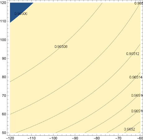
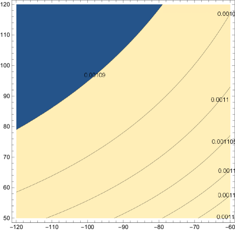
Figure 1: Contour plots of the spectral index of scalar perturbations $n_{S}$ (left) and the tensor-to-scalar ratio $r$ (right) depending on parameters $\gamma$ and $\Lambda$. Their values range from [-120,-60] and [50,120] respectively. These plots indicate that even though a dependence is observed, the numerical value changes by a fraction in each case.

Examining the correspondence of the system under a change in the values of the free parameters, once finds that the constant-roll parameter $\beta$ has the most impact on the results while $\Lambda$ and $\gamma$ influence them as well but not at a significant rate as the first. For instance, we mention that changing $\beta$ from -0.008 to -0.005, the spectral index of primordial curvature perturbations obtains the value $n_{S}=0.959128$ which makes this value incompatible with the observations. We also note that the tensor-to-scalar ratio experiences a change as well, but it decreases its value so it remains acceptable. On the other hand, $\Lambda$ changes the results but only when its order of magnitude alters and not its sign. Numerically speaking, the value $\Lambda=-100$ produces the results $n_{S}=0.964947$ and $r=0.00106215$ while $\Lambda=1$ gives $n_{S}=0.969504$ and $r=0.0024329$, which is a more significant change than the one produced by flipping the sign. The same applies to $\gamma$ as $\gamma=100$ gives the values $n_{S}=0.964947$, $r=0.00106215$ while $\gamma=-1$ the values $n_{S}=0.969504$ and $r=0.00243129$. This in turn implies that $\Lambda$ and $\gamma$ have a similar behavior as the same changes lead to the exact same numerical values. However, the most dominant parameter which is also the decisive factor remains the constant-roll parameter. The phenomenology of the model is depicted in Fig. 1 for some ranges of values of the free parameters.

In a similar manner, the same parameters define the amount of non-Gaussianities as well. This time however, the effects are reversed. Each change in the parameters, as before, leads only to an insignificant change in the fourth decimal (or even lesser) of the value of the non linear term $f_{NL}^{eq}$. Furthermore, constant-roll parameter $\beta$ has the same result in the three-point correlator. However, $\Lambda$ and $\gamma$ now lead to significant changes in the three-point correlator, since changing $\Lambda=1$ leads to the value $\left<\mathcal{R}^{2}\right>=67.967$ and changing $\gamma=-1$ leads to $\left<\mathcal{R}^{2}\right>=6.7967\cdot 10^{-15}$. Thus, the order of magnitude of the three-point correlator depends greatly on $\Lambda$, $\gamma$ and in fact $V_{0}$, since the correlator is proportional to squared Hubble’s parameter. This is also the reason why the constant in Ricci’s coupling function affects its order of magnitude as well. For example, a decrease in the amplitude of the scalar potential by two orders leads to a decrease in the order of magnitude of the three point correlator by four orders.

Due to this particular choice of parameters, the exponent of the scalar potential in Eq. (55) is 2.0001, which is really close to 2. Hence, this particular model can be thought of as a linear Ricci coupling, squared power-law potential and exponential Gauss-Bonnet coupling function, which in principle is a simple case. In other words, the simplest case in the choice of coupling functions leads to a simple scalar potential as well. However, this is not a universal characteristic, but rather a model dependent one. If one were to use a different approach for Hubble’s parameter then the resulting scalar potential may not have been that simple.

Finally, we examine the validity of the approximations which were made necessarily in order to solve approximately the system of equations of motion. Referring to the slow-roll approximations which were assumed, we mention that during the first horizon crossing, $\dot{H}/H^{2}\sim\mathcal{O}(10^{-3})$, $\frac{1}{2}\omega\dot{\phi}^{2}\sim\mathcal{O}(10^{-10})$ and $V\sim\mathcal{O}(10^{-3})$ which indicates that indeed the slow-roll approximations do apply. However, these were not the only approximations assumed in the equations of motion. Recalling our previous statements, we mentioned that the string corrective terms in each separate equation of motion will be omitted. This again is a valid assumption, as it turns out that $24\dot{\xi}H^{3}\sim\mathcal{O}(10^{-39})$, $16\dot{\xi}H\dot{H}\sim\mathcal{O}(10^{-41})$ and $24\xi^{\prime}H^{4}\sim\mathcal{O}(10^{-37})$ which justifies why, compared to the rest terms in Equations (3), (4) and (5) respectively were omitted.

IV.2 Model II: Trigonometric and Power Law Couplings

Suppose now that the scalar coupling functions are defined as,

$$\centering h(\phi)=\Lambda\sin(\gamma\kappa\phi+\theta),\,\@add@centering$$ (66)

$$\centering\xi(\phi)=\lambda(\kappa\phi)^{m}.\,\@add@centering$$ (67)

This model was studied also in the slow-roll case in Ref. Odintsov:2020xji and was deemed as a false positive model, as it generated compatible results while simultaneously violating the approximations made in the equations of motion. This is a bizarre choice for the Ricci coupling constant so it was tempting to study the viability of the same model under the constant-roll condition. For the equations of motion, we choose,

$$\centering H^{2}\simeq\frac{\kappa^{2}V}{3(1-\beta)h^{\prime}}\frac{\xi^{\prime\prime}}{\xi^{\prime}},\,\@add@centering$$ (68)

$$\centering\dot{H}\simeq-\frac{H^{2}}{2}(1-\beta)^{2}\frac{h^{\prime\prime}}{h}\left(\frac{\xi^{\prime}}{\xi^{\prime\prime}}\right)^{2},\,\@add@centering$$ (69)

$$\centering V^{\prime}+3H^{2}\left(\omega(1-\beta)(1+\frac{\beta}{3})\frac{\xi^{\prime}}{\xi^{\prime\prime}}-2\frac{h^{\prime}}{\kappa^{2}}\right)\simeq 0.\,\@add@centering$$ (70)

It is clear that the trigonometric choice is perfect for such approach since is simplifies greatly the ratio of the Ricci coupling and in addition, since its second derivative is negative, it is convenient to choose the positive sign of index $\epsilon_{1}$. From this choice of coupling constant, it turns out that the scalar potential is,

$$\centering V(\phi)=V_{0}(\kappa\phi)^{\alpha_{1}}\left(\frac{\cos(\frac{\gamma\kappa\phi+\theta}{2})-\sin(\frac{\gamma\kappa\phi+\theta}{2})}{\cos(\frac{\gamma\kappa\phi+\theta}{2})+\sin(\frac{\gamma\kappa\phi+\theta}{2})}\right)^{\alpha_{2}},\,\@add@centering$$ (71)

where $\alpha_{1}=\frac{2(m-1)}{1-\beta}$ and $\alpha_{2}=\frac{\omega(3+\beta)}{3\Lambda\gamma^{2}}$. It is the same form as in the slow-roll condition where now the constant-roll parameter $\beta$ appears in the exponents. The same obviously applies to the rest parameters as well,

$$\centering\delta_{X}=\frac{\omega}{2h(\phi)}\left(\frac{(1-\beta)\kappa\phi}{m-1}\right)^{2},\,\@add@centering$$ (72)

$$\centering\delta_{\xi}\simeq m(1-\beta)\frac{\xi(\phi)}{h(\phi)}\frac{\kappa^{4}V(\phi)}{3\gamma\kappa\phi\Lambda\cos(\gamma\kappa\phi+\theta)},\,\@add@centering$$ (73)

$$\centering\epsilon_{s}\simeq\left(\frac{(1-\beta)\gamma\kappa\phi}{m-1}\right)^{2}+\frac{1-\beta}{(m-1)h(\phi)}\left(\frac{\Lambda\gamma\kappa\phi\cos(\gamma\kappa\phi+\theta)}{2}-\frac{4m\xi(\phi)\kappa^{4}V(\phi)}{3h(\phi)}\right),\,\@add@centering$$ (74)

$$\centering\epsilon_{1}\simeq\frac{1}{2}\left(\frac{(1-\beta)\gamma\kappa\phi}{m-1}\right)^{2},\,\@add@centering$$ (75)

$$\centering\epsilon_{2}=\beta,\,\@add@centering$$ (76)

$$\centering\epsilon_{3}=\frac{(1-\beta)\gamma\kappa\phi\cot(\gamma\kappa\phi+\theta)}{2(m-1)},\,\@add@centering$$ (77)

$$\centering\epsilon_{5}=\frac{3(\beta-1)\gamma^{2}\kappa\Lambda^{2}\phi^{2}\cos^{2}(\gamma\kappa\phi+\theta)+8\kappa^{3}\lambda(m-1)mV(\phi)(\kappa\phi)^{m}}{(m-1)\left(16\kappa^{3}\lambda mV(\phi)(\kappa\phi)^{m}-3\gamma\Lambda^{2}\phi\sin(2(\gamma\kappa\phi+\theta))\right)},\,\@add@centering$$ (78)

$$\centering\epsilon_{6}\simeq\epsilon_{5}.\,\@add@centering$$ (79)

In this case, even $\epsilon_{6}$ has a gory form so invoking the slow-roll approximations, this index must be equal to $\epsilon_{5}$. Finally we note that the values of the scalar field at the initial and final stage of inflation are,

$$\centering\phi_{f}=\pm\frac{\sqrt{2}}{\kappa}\left|\frac{m-1}{\gamma(1-\beta)}\right|,\,\@add@centering$$ (80)

$$\centering\phi_{i}=\phi_{f}e^{-\frac{N(1-\beta)}{m-1}}.\,\@add@centering$$ (81)

Here, we shall implement the positive value of $\phi_{f}$ and in consequence, $\phi_{i}$. Letting ($\omega$, $\Lambda$, $\lambda$, $V_{0}$, $N$, $m$, $\gamma$, $\theta$, $\beta$)=(1, 0.1, $10^{-14}$, $10^{33}$, 60, 6, 2.5, $\frac{\pi}{6}$, 0.0174) then the produced results are $n_{S}=0.965218$, $n_{T}=-0.0000185$ and $r=0.0001483$ which are compatible with the latest observations. In addition, the predicted values for the non-Gaussianities are $f_{NL}^{eq}=0.0818867$ and $\left<\mathcal{R}^{3}\right>=2.03855\cdot 10^{-6}$ with a corresponding deviation $\mathcal{S}\sim 3.14567\cdot 10^{-11}$ from the Gaussian distribution. The scalar field now seems to increase with time since $\phi_{i}=0.00002179$ and $\phi_{f}=2.87851$ and furthermore, the slow-roll criteria apply more than enough since $\epsilon_{1}=5.73184\cdot 10^{-11}$, $\epsilon_{3}=9.27124\cdot 10^{-6}$, $\epsilon_{4}=2.40493\cdot 10^{-7}$, $\epsilon_{5}=9.27124\cdot 10^{-6}=\epsilon_{6}$. Moreover $\delta_{\xi}=1.35\cdot 10^{-50}$, $\delta_{X}=9.8356\cdot 10^{-20}$, $\epsilon_{s}=9.27118\cdot 10^{-6}$, $s=-1.67\cdot 10^{-40}$ and $\eta=0.196494$ which goes to say that only one parameter is dominant.

However, even in the constant-roll case, the model is in fact false since certain approximations are invalid, We note that the slow-roll conditions do apply, however in order to derive equation (68) from (3), we made the assumption that the term $Hh^{\prime}$ is more dominant than the term $H^{2}h$, a reasonable assumption which is unfortunately invalid as $Hh^{\prime}\sim\mathcal{O}(10^{-15})$ while $H^{2}h\sim\mathcal{O}(10^{-11})$, hence the latter is more dominant and cannot be discarded. Nevertheless, even if a single approximation does not apply, the model is automatically rendered invalid, no matter the beauty or functionality it may contain. Perhaps a different set of values for the free parameters could save this model in the end.

It is intriguing however to examine whether using a different form for Hubble’s parameter, mainly the condition which was invalid, could manifest viable results. We shall also make a different assumption as in the previous, where we neglect the ratio $\xi^{\prime}/\xi^{\prime\prime}$ in the differential equation of the scalar potential. Suppose now that,

$$\centering H^{2}\simeq\frac{\kappa^{2}V}{3h},\,\@add@centering$$ (82)

$$\centering V^{\prime}-6H^{2}\frac{h^{\prime}}{\kappa^{2}}\simeq 0.\,\@add@centering$$ (83)

Subsequently, the scalar potential reads,

$$\centering V(\phi)=V_{0}\sin(\gamma\kappa\phi+\theta)^{2},\,\@add@centering$$ (84)

where for consistency, the integration constant $V_{0}$ has mass dimensions [m]⁴. A quick comparison between the two potentials indicates that in the second approach, the potential is functionally more elegant. This can be attributed to the change in the differential equation of the scalar field and not the change in Hubble’s parameter. Furthermore, changing Hubble and also keeping the ratio $\xi^{\prime}/\xi^{\prime\prime}$ in the differential equation results in a perplexed potential similar to the previous case. Hence, this simplification in the scalar potential is a universal feat of this particular formalism we decided to work and is not model dependent.

Concerning the auxiliary parameters and the slow-roll indices, we mention that since they depend strongly on the form of the coupling functions, no change is expected apart from the form of $\delta_{\xi}$, $\epsilon_{s}$ and indices $\epsilon_{5}$ and $\epsilon_{6}$,

$$\centering\delta_{\xi}\simeq\frac{m(1-\beta)}{3(m-1)}\frac{\xi(\phi)}{h(\phi)}\kappa^{4}V(\phi),\,\@add@centering$$ (85)

$$\centering\epsilon_{s}\simeq\left(\frac{(1-\beta)\gamma\kappa\phi}{m-1}\right)^{2}+\frac{1-\beta}{(m-1)h(\phi)}\left(\frac{\Lambda\gamma\kappa\phi\cos(\gamma\kappa\phi+\theta)}{2}-\frac{4m\xi(\phi)\kappa^{4}V(\phi)}{3h(\phi)}\right),\,\@add@centering$$ (86)

$$\centering\epsilon_{5}=\frac{(1-\beta)\left(8\lambda m\kappa^{4}V(\phi)(\kappa\phi)^{m}\csc^{2}(\gamma\kappa\phi+\theta)-3\gamma\Lambda^{2}\kappa\phi\cot(\gamma\kappa\phi+\theta)\right)}{16(1-\beta)\lambda m\kappa^{4}V(\varphi)(\kappa\varphi)^{m}\csc^{2}(\gamma\kappa\phi+\theta)-6\Lambda^{2}(m-1)},\,\@add@centering$$ (87)

$$\centering\epsilon_{6}=\frac{(1-\beta)\left(3\gamma\Lambda^{2}(m-1)\kappa\phi\sin(2(\gamma\kappa\phi+\theta))-16(1-\beta)\lambda m(\kappa\phi)^{m}\left(\kappa^{4}V(\phi)(m-\gamma\kappa\phi\cot(\gamma\kappa\phi+\theta))+\kappa\varphi\kappa^{3}V^{\prime}(\phi)\right)\right)}{4(m-1)\left(3\Lambda^{2}(m-1)\sin^{2}(\gamma\kappa\phi+\theta)-8(1-\beta)\lambda m\kappa^{4}V(\phi)(\kappa\phi)^{m}\right)}.\,\@add@centering$$ (88)

The same applies to the expressions of the values for the scalar field. Thus, designating the exact same values of parameters as before, with the only exception being parameters $\Lambda$ and $V_{0}$ which are now assigned the values $\Lambda=0.4$ and $V_{0}=10^{-6}$ leads to compatible results as $n_{s}=0.965226$, $n_{T}=-0.00001854$ and $r=0.0001483$ are acceptable. Moreover, the non-Gaussianities of the model are expected to obtain the values $f_{NL}^{eq}=0.0818867$ and $\left<\mathcal{R}^{3}\right>=0.0769239$, with a corresponding skewness $\mathcal{S}\sim 0.00001654$. This is a completely different expected amount of deviation from previously but still very small as expected.

Unfortunately, even this case is not viable since a single approximation is violated. We mention that $h^{\prime\prime}\dot{\phi}^{2}\sim\mathcal{O}(10^{-18})$ while $H\dot{h}\sim\mathcal{O}(10^{-12})$, hence the form of Hubble’s derivative in Eq. (69) is not justifiable.

IV.3 Model III: Power-Law and Exponential Couplings

In this case, we shall examine a model reminiscing the first one presented, but this time the Ricci coupling will be generalized. Let,

$$\centering h(\phi)=\Lambda(\kappa\phi)^{m},\,\@add@centering$$ (89)

$$\centering\xi(\phi)=\lambda e^{\gamma\kappa\phi}.\,\@add@centering$$ (90)

This choice is made similarly due to the simple ratios in the coupling functions. Furthermore, we shall use the following forms of the equations of motion,

$$\centering H^{2}\simeq\frac{\kappa^{2}V}{3h\left(1+(1-\beta)\frac{h^{\prime}}{h}\frac{\xi^{\prime}}{\xi^{\prime\prime}}\right)},\,\@add@centering$$ (91)

$$\centering\dot{H}\simeq\frac{H^{2}}{2}(1-\beta)^{2}\frac{\xi^{\prime}}{\xi^{\prime\prime}}\left(\frac{h^{\prime}}{h}-\frac{h^{\prime\prime}}{h}\frac{\xi^{\prime}}{\xi^{\prime\prime}}\right),\,\@add@centering$$ (92)

$$\centering V^{\prime}-6H^{2}\frac{h^{\prime}}{\kappa^{2}}\simeq 0.\,\@add@centering$$ (93)

Here, it is convenient to make use of the positive sign of slow-roll index $\epsilon_{1}$. Also, we shall use the more simplified differential equation for the scalar potential since, as mentioned before, leads to functionally more elegant results. In fact, the scalar potential now is,

$$\centering V(\phi)=V_{0}(m(1-\beta)+\gamma\kappa\phi)^{2m},\,\@add@centering$$ (94)

where similarly, the integration constant $V_{0}$ has again mass dimensions [m]⁴. In addition, the auxiliary parameters and slow-roll indices are written as,

$$\centering\delta_{X}=\frac{\omega(1-\beta)^{2}}{2\gamma^{2}h(\phi)},\,\@add@centering$$ (95)

$$\centering\delta_{\xi}\simeq\frac{1-\beta}{3}\frac{\xi(\phi)}{h^{2}(\phi)}\frac{\kappa^{2}V(\phi)}{\left(1+\frac{m(1-\beta)}{\gamma\kappa\phi}\right)},\,\@add@centering$$ (96)

$$\centering\epsilon_{s}\simeq-\frac{m(1-\beta)^{2}}{2\gamma\kappa\phi}\left(1-\frac{m-1}{\gamma\kappa\phi}\right)+(1-\beta)\left(\frac{m}{\gamma\kappa\phi}-\frac{4\xi(\phi)\kappa^{4}V(\phi)}{3h^{2}(\phi)\left(1+\frac{m(1-\beta)}{\gamma\kappa\phi}\right)}\right),\,\@add@centering$$ (97)

$$\centering\epsilon_{1}\simeq-\frac{m(1-m-\gamma\kappa\phi)}{2}\left(\frac{1-\beta}{\gamma\kappa\phi}\right)^{2},\,\@add@centering$$ (98)

$$\centering\epsilon_{2}=\beta,\,\@add@centering$$ (99)

$$\centering\epsilon_{3}=\frac{m(1-\beta)}{2\gamma\kappa\phi},\,\@add@centering$$ (100)

$$\centering\epsilon_{5}=\frac{(\beta-1)\left(3\Lambda^{2}m(\kappa\phi)^{2m}((\beta-1)m-\gamma\kappa\phi)+2\lambda(2\gamma\kappa\phi)^{2}\kappa^{4}V(\phi)e^{\gamma\kappa\phi}\right)}{2\gamma\kappa\phi\left(8(\beta-1)\gamma\kappa\phi\lambda\kappa^{4}V(\phi)e^{\gamma\kappa\phi}-3\Lambda^{2}(\kappa\phi)^{2m}((\beta-1)m-\gamma\kappa\phi)\right)},\,\@add@centering$$

$$\centering\epsilon_{6}\simeq\epsilon_{5}.\,\@add@centering$$ (101)

This choice leads to a second order polynomial slow-roll index $\epsilon_{1}$ hence two values of the scalar field at the end of inflation appear, once the index $\epsilon_{1}$ becomes of order $\mathcal{O}(1)$. These values are showcased below,

$$\centering\phi_{f}=\frac{(1-\beta)\sqrt{m}\left((1-\beta)\sqrt{m}\pm\sqrt{\left(\beta^{2}-2\beta-7\right)m+8}\right)}{4\gamma\kappa}.\,\@add@centering$$ (102)

In order to derive the expression of the initial value of the scalar field from Eq. (31). we shall assume the first case with the plus sign. As a result, the formula for the initial value is,

$$\centering\phi_{i}=\frac{(1-\beta)\left((1-\beta)m-4N-\sqrt{m}\sqrt{\left(\beta^{2}-2\beta-7\right)m+8}\right)}{4\gamma\kappa}.\,\@add@centering$$ (103)

Assigning the following values ($\omega$, $\Lambda$, $\lambda$, $V_{0}$, $N$, $m$, $\gamma$, $\beta$)=(1, 1650, $10^{-4}$, $10^{-6}$, 60, 0.5, -2, 0.0001) produces viable results as $n_{S}=0.963545$, $n_{T}=0.00006998$ and $r=0.00055759$ are compatible with the observations. Furthermore, for the non-Gaussianities, $f_{NL}^{eq}$=0.0136957 and $\left<\mathcal{R}^{3}\right>=1.25\cdot 10^{-17}$, extremely small values with a corresponding predicted deviation of $\mathcal{S}\sim 4.784\cdot 10^{-25}$, which in turn implies that there exists no effective deviation. Concerning the slow-roll indices, we mention that the slow-roll criteria are indeed true as $\epsilon_{1}=-0.004114$, $\epsilon_{3}=-0.004149$, $\epsilon_{4}=0.005674$, $\epsilon_{5}=-0.004149=\epsilon_{6}$ and also, the auxiliary parameters for evaluating the non-Gaussianities obtain the values $\delta_{\xi}=-1.679\cdot 10^{-43}$, $\delta_{X}=-3.0603\cdot 10^{-14}$, $\eta=0.0329975$, $\epsilon_{s}=-0.00003484$ and $s=-1.1716\cdot 10^{-33}$ which are extremely small values. Finally, for the scalar field we note that $\phi_{i}=30.122$ while $\phi_{f}=0.125$ which shows a decrease with time. The inflationary phenomenology of the model at hand is presented in Figs. 2 and LABEL:parplot2 for some ranges of values of the free parameters.

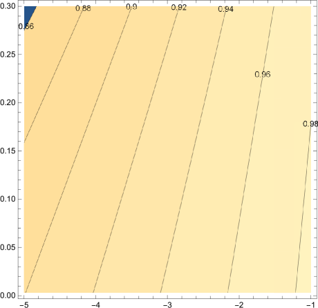
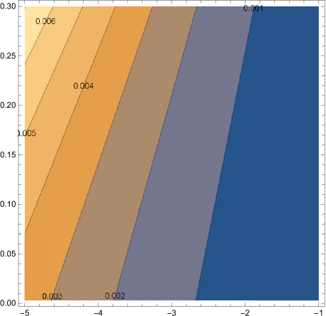
Figure 2: Contour plots of the spectral index of scalar perturbations $n_{S}$ (left) and the tensor-to-scalar ratio $r$ (right) depending on parameters $\beta$ and $\gamma$. Their values range from [0.003, 0.3] and [-5,-1] respectively. It is clear that the both objects depend strongly on each parameter.

Figure 3: Parametric plot of spectral index of scalar perturbations $n_{S}$ (x axis) and the tensor-to-scalar ratio $r$ (y axis) depending on parameters $\beta$ and $\gamma$. Their values range from [0.0003, 0.001] and [-75,-1] respectively. There exists a one-on one correlation between these quantities and a variety of possible set of values. The compatible with the observations results are on the bottom right.

This model has interesting dynamics, since altering some values yields different characteristics. For instance, we mention that $\gamma$ must be negative, otherwise the value of the scalar field during the first horizon crossing becomes negative and subsequently, the spectral indices obtain an imaginary part where in certain cases is even grater, in absolute value, than the real part. The same applies to the exponent $m$ for each value, positive or negative, small or large. Only when $m=0.5$ the model yields real numbers and in fact, changing both $m$ and $\gamma$ does not negate the appearance of complex numbers. Moreover, the constant-roll parameter $\beta$ influences greatly the spectral index of scalar perturbations and in second terms the tensor-to-scalar ratio as designating the value $\beta=0.001$ leads to $n_{S}=0.961747$ and $r=0.000617343$, so $\beta$ plays significant role. This particular parameter can also obtain negative values and still lead to viable results. In contrast, $\Lambda$ alters only the spectral index of primordial curvature perturbations as taking the value $\Lambda=1450$ leads to $n_{s}=0.964103$ and $\Lambda=450$ to $n_{S}=0.9706$. Changing the sign of $\Lambda$ also influences the spectral index in the same manner. Lastly, decreasing $\gamma$ leads to a subsequent decrease in the spectral index of scalar perturbations while simultaneously keeping the tensor-to-scalar invariant. The tensor-to-scalar ratio is very strictly assigned as only the constant-roll parameter changes is and not significantly as we showed previously. The decisive factor is the exponent $m$ and the fact that only one value leads to not only real numbers, but also a viable tensor-to-scalar ratio is fascinating.

Concerning the non-Gaussianities, $\beta$ alters only the numerical value and not the order of magnitude of both the non linear term and the three-point correlator. On the other hand, decreasing $\gamma$, for instance to the value $\gamma=20$ increases the order of magnitude of the three-point correlator approximately three orders, while leaving invariant non-linear term. Finally, as expected, parameters $\Lambda$ and $V_{0}$ influence the order of magnitude of the three point correlator. Again, this is attributed to Hubble’s parameter and the connection it has with the three-point correlator.

This description seems to be correct since all the approximations made actually do apply, but in certain cases marginally, We mention that for the slow-roll conditions, $\dot{H}/H^{2}\sim\mathcal{O}(10^{-3})$ and additionally, $X/V\sim\mathcal{O}(10^{-6})$ so indeed they apply. Moreover, for the equations of motion (91) and (93) we note that $24\dot{\xi}H^{3}\sim\mathcal{O}(10^{-47})$ and $24\xi^{\prime}H^{4}\sim\mathcal{O}(10^{-46})$ so it justifies why the string corrections where omitted in equations (3) and (5) respectively. Also, $h^{\prime}\sim\mathcal{O}(10^{2})$ while $\xi^{\prime}/\xi^{\prime\prime}\sim\mathcal{O}(10^{-1})$ so the extra approximation does indeed apply. Lastly, for Eq. (92), we note that $16\dot{\xi}H\dot{H}\sim\mathcal{O}(10^{-50})$ while the terms used in our approach, meaning $H\dot{h}$ and $h^{\prime\prime}\dot{\phi}^{2}$ are of order $\mathcal{O}(10^{-7})$ and $\mathcal{O}(10^{-9})$ respectively so it justifies why the string corrective term was neglected. However, the kinetic term $\dot{\phi}^{2}$ which was discarded as well happens to be of order $\mathcal{O}(10^{-10})$ so it is quite close to the term $h^{\prime\prime}\dot{\phi}^{2}$. However, we can thing such term as a first correction of the same model but with an expression for Hubble’s derivative exactly as in the previous model II. Therefore, adding the term $h^{\prime\prime}\dot{\phi}^{2}$ in order to get a better understanding and treating it as a first order corrective term and not as dominant as the term $H\dot{h}$ makes sense. For the sake of completeness we mention that one can overcome such obstacle when working in the non-canonical case. Assuming for instance that $\omega=0.001$ and changing the constant-roll parameter to the value $\beta=-0.005$ leads again to viable results while keeping the orders of magnitude of each element exactly as before, with the only exception being the kinetic term. Then these terms become truly dominant compared to the rest.

Let us now compare the previous model with the slow-roll case. As was the case with model I, letting $\beta=0$ and changing $\epsilon_{2}$ leads to, as expected, the exact same potential. Changing only one parameter, $\gamma=-20$, leads to compatible results as $n_{S}=0.966737$, $n_{T}=0.0000703$, $r=0.0005602$, $f_{NL}^{eq}=0.0138935$, $\left<\mathcal{R}^{3}\right>=1.26423\cdot 10^{-15}$ and $\mathcal{S}\sim 1.51686\cdot 10^{-22}$ Hence, both approaches yield viable phenomenology. This is expected since $\beta$ obtains small values, hence $\ddot{\phi}$ can in fact be discarded in Eq. (4) as was the case with the slow-roll condition. However it is worth inspecting the constant-roll case, even if it produces similar results since both conditions are intrinsically different.

V Panorama of All Possible Approximations During the Inflationary Era and Their Validity

In this section, we summarize all the possible approaches one can use when studying the inflationary era of a non-minimally coupled model supplemented with string correction terms under the constant-roll condition. Each one is accompanied by the approximations that must apply during the first horizon crossing. As it was shown previously, there exist multiple different approaches in each separate equation of motion one can work with, each one promising and capable of leading to functional expressions. Despite the choice, one must always check whether the approximations made in the model apply, simply because even a single invalid approximation renders the model false, even if it is capable of producing viable results.

Before elaborating any further, it is worth mentioning that no matter the choices for the equations, there exist two approximations which must apply no matter the case. Previously, during our analysis in the viability of certain models, we were free to change our approach if stumbled on a violating condition although this is indicative of the flexibility this formalism contains. However, no matter the choice, the slow-roll conditions must always apply, meaning that in every model, the following relations must be respected,

$$\centering\dot{H}\@add@centering \ll H^{2}, \frac{1}{2}\omega\dot{\phi}^{2} \ll V.\,$$ (104)

In other words, these are the main approximations that must apply no matter the case while the rest approximations are auxiliary, in order to make the system of equations solvable. Consequently, it is worth inspecting them separately in each equation of motion.

For the differential equation of the scalar potential, we mention that there exist two possible ways one can work with easily, as shown below,

$$\centering V^{\prime}+3H^{2}\left(\omega(1-\beta)(1+\frac{\beta}{3})\frac{\xi^{\prime}}{\xi^{\prime\prime}}-2\frac{h^{\prime}}{\kappa^{2}}\right)\simeq 0,\,\@add@centering$$ (105)

$$\centering V^{\prime}-6H^{2}\frac{h^{\prime}}{\kappa^{2}}\simeq 0.\@add@centering$$ (106)

Working with the full expression as Eq. (12) is always a possibility but adding more terms in the differential equation which are also less dominant make the form of the scalar potential perplexed for no apparent reason, so it is convenient to discard them completely. For the corresponding approximations, one must check whether the following correlations hold,

$$\centering 24\xi^{\prime}H^{4}\@add@centering \ll V^{\prime}, 24\kappa\xi^{\prime}H^{2} \ll\kappa\xi^{\prime}/\xi^{\prime\prime}-2h^{\prime}, \kappa\xi^{\prime}/\xi^{\prime\prime} \ll h^{\prime}.\,$$ (107)

When a correlation contains multiple expressions on each side, one must always examine each term from the right separately which each term on the lest. Moreover, what matters is obviously the order of magnitude and not the sign of each term. Lastly, the last condition may be violated when one works with Eq. (105).

For the expression of Hubble’s parameter, one has the ability to choose from three possible expressions,

$$\centering H^{2}\simeq\frac{\kappa^{2}V}{3h\left(1+(1-\beta)\frac{h^{\prime}}{h}\frac{\xi^{\prime}}{\xi^{\prime\prime}}\right)},\,\@add@centering$$ (108)

$$\centering H^{2}\simeq\frac{\kappa^{2}V}{3h},\,\@add@centering$$ (109)

$$\centering H^{2}\simeq\frac{\kappa^{2}V}{3(1-\beta)h^{\prime}}\frac{\xi^{\prime\prime}}{\xi^{\prime}}.\,\@add@centering$$ (110)

As it was demonstrated in the previous model, there are cases in which one form is more preferable that the rest, so one must choose wisely. Also, the corresponding assumptions that must apply are,

$$\centering 14\kappa^{2}\dot{\xi}H^{3}\@add@centering \ll\kappa^{2}V-3H^{2}h-3H\dot{h}, H\dot{h} \ll hH^{2}, hH^{2} \ll H\dot{h}.\,$$ (111)

The last conditions may seem contradictory but we note that the second refers to equation (109) while the third to (110) so they make sense. In addition, the first approximation must apply always, in each form of Hubble’s parameter since in every single approach the string corrections were discarded.

Lastly, the expression for Hubble’s derivative is the most crucial as different approaches lead to different characteristics and therefore different values for the scalar field during the first horizon crossing, leading to subsequent different values for the observed quantities and the predicted non-Gaussianities. Thus, different choices lead to different phenomenology. When working under the constant-roll condition, one sees that the term $\ddot{\phi}h^{\prime}$ can also be included in the equation, a feature which can not be applies in the slow-roll case. Thus, there exist six inherently different forms, as presented below,

$$\centering\dot{H}\simeq\frac{H^{2}}{2}(1-\beta)^{2}\frac{h^{\prime}}{h}\frac{\xi^{\prime}}{\xi^{\prime\prime}},\,\@add@centering$$ (112)

$$\centering\dot{H}\simeq-\frac{H^{2}}{2}(1-\beta)^{2}\frac{h^{\prime\prime}}{h}\left(\frac{\xi^{\prime}}{\xi^{\prime\prime}}\right)^{2},\,\@add@centering$$ (113)

$$\centering\dot{H}\simeq-\frac{H^{2}}{2h}\kappa^{2}\omega(1-\beta)^{2}\left(\frac{\xi^{\prime}}{\xi^{\prime\prime}}\right)^{2},\,\@add@centering$$ (114)

$$\centering\dot{H}\simeq\frac{H^{2}}{2}(1-\beta)^{2}\frac{\xi^{\prime}}{\xi^{\prime\prime}}\left(\frac{h^{\prime}}{h}-\frac{h^{\prime\prime}}{h}\frac{\xi^{\prime}}{\xi^{\prime\prime}}\right),\,\@add@centering$$ (115)

$$\centering\dot{H}\simeq\frac{H^{2}}{2}(1-\beta)^{2}\frac{\xi^{\prime}}{\xi^{\prime\prime}}\left(\frac{h^{\prime}}{h}-\frac{\kappa^{2}\omega}{h}\frac{\xi^{\prime}}{\xi^{\prime\prime}}\right),\,\@add@centering$$ (116)

$$\centering\dot{H}\simeq-\frac{H^{2}}{2}(1-\beta)^{2}\left(\frac{\xi^{\prime}}{\xi^{\prime\prime}}\right)^{2}\left(\frac{\kappa^{2}\omega}{h}+\frac{h^{\prime\prime}}{h}\right).\,\@add@centering$$ (117)

These are all the possible forms of Hubble’s derivative. There exists also the possibility of keeping every term of (4) apart from the string correction and for with such model. This is attributed to the constant-roll condition which now enables us to work with a functional form of the term $\ddot{\phi}$. However this case is very intricate and if it is solvable, it might by only for the simplest case like a power-law expression. Such case could correspond to the first model as well where the linear choice for Ricci’s coupling function discarded naturally the second derivative. Nevertheless, it is wise to present the simplified choices as well since in many models as showcased previously, certain terms are not so dominant and in fact can be neglected. Let us now proceed with the corresponding approximations for each model separately.

Working with Eq. (112), the results must respect the following conditions,

$$\centering 16\kappa^{2}\dot{\xi}H\@add@centering \ll 2h, (\kappa^{2}\omega+h^{\prime\prime})\dot{\phi} \ll(1-\beta)Hh^{\prime}.\,$$ (118)

In a similar way, choosing Eq. (113), we get the following conditions,

$$\centering 16\kappa^{2}\dot{\xi}H\@add@centering \ll 2h, \kappa^{2}\omega \ll h^{\prime\prime}, (1-\beta)Hh^{\prime} \ll\kappa^{2}h^{\prime\prime}\dot{\phi}.\,$$ (119)

In the case of Eq. (114), we have,

$$\centering 16\kappa^{2}\dot{\xi}H\@add@centering \ll 2h, h^{\prime\prime} \ll\kappa^{2}\omega, (1-\beta)Hh^{\prime} \ll\kappa^{2}\dot{\phi}.\,$$ (120)

If one were to work with Eq. (115), then,

$$\centering 16\kappa^{2}\dot{\xi}H\@add@centering \ll 2h, \kappa^{2}\omega\dot{\phi} \ll(1-\beta)Hh^{\prime}-h^{\prime\prime}\dot{\phi}.$$ (121)

The choice of Eq. (116) demands the following conditions hold true,

$$\centering 16\kappa^{2}\dot{\xi}H\@add@centering \ll 2h, h^{\prime\prime}\dot{\phi} \ll(1-\beta)Hh^{\prime}-\kappa^{2}\omega\dot{\phi}.\,$$ (122)

Finally, the last choice of Eq. (117) leads to the following expressions,

$$\centering 16\kappa^{2}\dot{\xi}H\@add@centering \ll 2h, (1-\beta)Hh^{\prime} \ll(\kappa^{2}\omega+h^{\prime\prime})\dot{\phi}.\,$$ (123)

The first condition is the same in each choice and it simply states that we chose Hubble’s derivative from the term $2h\dot{H}$ and not the string corrections. This was also done in the case of Hubble’s parameter itself were the string correction, which was proportional toy $H^{3}$ was discarded in each case. These are all the possible approaches one must follow. Each condition written here for each case must be respected and once again, we note that the order of magnitude matters and not the sign itself. If these assumptions hold during the first horizon crossing, then the model is indeed viable.

VI Conclusions

In this paper, we studied the viability of a non-minimally coupled Einstein-Gauss-Bonnet gravity with the constant-roll condition holding true during the inflationary era. We presented a new framework, in which constraints of the velocity of the primordial tensor perturbations of the metric, which are essential in order for a model not to be at variance with the physical world. This constraint leads to a decrease in the degrees of freedom and subsequently to interesting dynamics. Here, we assumed for convenience that the scalar potential, which is in fact present in this framework, is not freely designated but on the contrary is derivable from the equations of motion once the scalar functions coupled to the Ricci scalar and Gauss-Bonnet invariant are specified. However, a completely different approach where one of the coupling functions is derived from the equations of motion is also feasible but was not studied further. We presented all the possible approximations which can be implemented and showed that each one is capable of producing different phenomenology, in certain cases even elegantly. The main result that is extracted from this paper is that even though the constant-roll is intrinsically different from the slow-roll assumption, both approaches are more than capable of producing viable phenomenology during the inflationary era, however, the non-Gaussianities predicted are small, a feature that we did not anticipate, since the constant-roll evolution is known to produce larger non-Gaussianities compared to the slow-roll case.

Appendix

We introduce a simple and elegant way of deriving a functional expression of $\xi(\phi)$. In each approach, it was shown that this particular functions appears in ratios, hence simplifying the ratios facilitates our study greatly. As a result, the first slow-roll index, the $e$-foldings number and the initial and final value of the scalar field have simple forms. The only requirement is that the coupling scalar function is at least three times differentiable. This particular formalism is shown below,

$$\centering\xi^{\prime}(\phi)=\kappa\lambda e^{\int{\kappa X[\phi]d\phi}},\,\@add@centering$$ (124)

where $\lambda$ is a dimensionless parameter and $X[\phi]$ is dimensionless arbitrary expression depending on the scalar field. This form was chosen simply because by differentiation with respect to the scalar field, we end up with the following expression,

$$\centering\xi^{\prime\prime}=\kappa X[\phi]\xi^{\prime}.\,\@add@centering$$ (125)

Thus, the ratio $\xi^{\prime}/\xi^{\prime\prime}$ which appears in all equations is replaced by the term $X[\phi]$. Choosing appropriately this term leads to an easy phenomenology. One can choose to work with such term in order to find an appealing and functional formula for the initial value of the scalar field $\phi$ and then later derive the expression of the Gauss-Bonnet coupling scalar function by simply integrating Eq. (124).

The same applies to the Ricci coupling function as well. Recall that in certain approaches, the function participates in the form of a ratio $h^{\prime}/h$, so extending the previous formalism, one can work with the form,

$$\centering h(\phi)=\Lambda e^{\int{\kappa Y[\phi]d\phi}},\,\@add@centering$$ (126)

where $\Lambda$ a dimensionless constant and $Y[\phi]$ a dimensionless arbitrary function of the scalar field. As was with the previous case,

$$\centering h^{\prime}=\kappa Y[\phi]h.\,\@add@centering$$ (127)

Thus, specifying $Y[\phi]$ determines the ratio for Ricci’s coupling function while simultaneously designating its form. Note that changing $\Lambda$ or $\lambda$ does not affect the form of the ratio of the coupling functions, or in this case $X[\phi]$ and $Y[\phi]$. Lastly, concerning a different ratio of the Ricci coupling function, the same approach still applies, although in this case the resulting equation is different. Now,

$$\centering\frac{h^{\prime\prime}}{h}=(\kappa Y[\phi])^{2}+\kappa Y^{\prime}[\phi],\,\@add@centering$$ (128)

so choosing an appropriate function which satisfies the above equation can simplify the results greatly. For instance, a linear choice for $Y[\phi]$ results in an exponential of a trigonometric function which makes this ratio constant, as was the case with the second model.

In view of this formalism, one is capable of working the other way around. Instead of guessing the coupling functions, the user chooses what they think of as an appropriate feature for the ratio and once this designating yields functional or elegant results, work backwards in order to find the coupling scalar functions responsible for such results. In the non minimal case, the task is more difficult since these two forms, $X[\phi]$ and $Y[\phi]$ could have constructive or destructive behavior so choosing wisely both is the key to elegant phenomenology. This is because choosing appropriately both forms could simplify greatly the results. The choice is obviously up to the reader.

References

- (1) J. c. Hwang and H. Noh, Phys. Rev. D 71 (2005) 063536 doi:10.1103/PhysRevD.71.063536 [gr-qc/0412126].
- (2) S. Nojiri, S. D. Odintsov and M. Sami, Phys. Rev. D 74 (2006) 046004 doi:10.1103/PhysRevD.74.046004 [hep-th/0605039].
- (3) G. Cognola, E. Elizalde, S. Nojiri, S. Odintsov and S. Zerbini, Phys. Rev. D 75 (2007) 086002 doi:10.1103/PhysRevD.75.086002 [hep-th/0611198].
- (4) S. Nojiri, S. D. Odintsov and M. Sasaki, Phys. Rev. D 71 (2005) 123509 doi:10.1103/PhysRevD.71.123509 [hep-th/0504052].
- (5) S. Nojiri and S. D. Odintsov, Phys. Lett. B 631 (2005) 1 doi:10.1016/j.physletb.2005.10.010 [hep-th/0508049].
- (6) M. Satoh, S. Kanno and J. Soda, Phys. Rev. D 77 (2008) 023526 doi:10.1103/PhysRevD.77.023526 [arXiv:0706.3585 [astro-ph]].
- (7) K. Bamba, A. N. Makarenko, A. N. Myagky and S. D. Odintsov, JCAP 1504 (2015) 001 doi:10.1088/1475-7516/2015/04/001 [arXiv:1411.3852 [hep-th]].
- (8) Z. Yi, Y. Gong and M. Sabir, Phys. Rev. D 98 (2018) no.8, 083521 doi:10.1103/PhysRevD.98.083521 [arXiv:1804.09116 [gr-qc]].
- (9) Z. K. Guo and D. J. Schwarz, Phys. Rev. D 80 (2009) 063523 doi:10.1103/PhysRevD.80.063523 [arXiv:0907.0427 [hep-th]].
- (10) Z. K. Guo and D. J. Schwarz, Phys. Rev. D 81 (2010) 123520 doi:10.1103/PhysRevD.81.123520 [arXiv:1001.1897 [hep-th]].
- (11) P. X. Jiang, J. W. Hu and Z. K. Guo, Phys. Rev. D 88 (2013) 123508 doi:10.1103/PhysRevD.88.123508 [arXiv:1310.5579 [hep-th]].
- (12) P. Kanti, R. Gannouji and N. Dadhich, Phys. Rev. D 92 (2015) no.4, 041302 doi:10.1103/PhysRevD.92.041302 [arXiv:1503.01579 [hep-th]].
- (13) C. van de Bruck, K. Dimopoulos, C. Longden and C. Owen, arXiv:1707.06839 [astro-ph.CO].
- (14) P. Kanti, J. Rizos and K. Tamvakis, Phys. Rev. D 59 (1999) 083512 doi:10.1103/PhysRevD.59.083512 [gr-qc/9806085].
- (15) E. O. Pozdeeva, M. R. Gangopadhyay, M. Sami, A. V. Toporensky and S. Y. Vernov, arXiv:2006.08027 [gr-qc].
- (16) I. Fomin, arXiv:2004.08065 [gr-qc].
- (17) M. De Laurentis, M. Paolella and S. Capozziello, Phys. Rev. D 91 (2015) no.8, 083531 doi:10.1103/PhysRevD.91.083531 [arXiv:1503.04659 [gr-qc]].
- (18) S. Chervon, I. Fomin, V. Yurov and A. Yurov, doi:10.1142/11405
- (19) K. Nozari and N. Rashidi, Phys. Rev. D 95 (2017) no.12, 123518 doi:10.1103/PhysRevD.95.123518 [arXiv:1705.02617 [astro-ph.CO]].
- (20) S. D. Odintsov and V. K. Oikonomou, Phys. Rev. D 98 (2018) no.4, 044039 doi:10.1103/PhysRevD.98.044039 [arXiv:1808.05045 [gr-qc]].
- (21) S. Kawai, M. a. Sakagami and J. Soda, Phys. Lett. B 437, 284 (1998) doi:10.1016/S0370-2693(98)00925-3 [gr-qc/9802033].
- (22) Z. Yi and Y. Gong, Universe 5 (2019) no.9, 200 doi:10.3390/universe5090200 [arXiv:1811.01625 [gr-qc]].
- (23) C. van de Bruck, K. Dimopoulos and C. Longden, Phys. Rev. D 94 (2016) no.2, 023506 doi:10.1103/PhysRevD.94.023506 [arXiv:1605.06350 [astro-ph.CO]].
- (24) B. Kleihaus, J. Kunz and P. Kanti, arXiv:1910.02121 [gr-qc].
- (25) A. Bakopoulos, P. Kanti and N. Pappas, Phys. Rev. D 101 (2020) no.4, 044026 doi:10.1103/PhysRevD.101.044026 [arXiv:1910.14637 [hep-th]].
- (26) K. i. Maeda, N. Ohta and R. Wakebe, Eur. Phys. J. C 72 (2012) 1949 doi:10.1140/epjc/s10052-012-1949-6 [arXiv:1111.3251 [hep-th]].
- (27) A. Bakopoulos, P. Kanti and N. Pappas, arXiv:2003.02473 [hep-th].
- (28) W. Ai, [arXiv:2004.02858 [gr-qc]].
- (29) S. D. Odintsov and V. K. Oikonomou, Phys. Lett. B 797 (2019) 134874 doi:10.1016/j.physletb.2019.134874 [arXiv:1908.07555 [gr-qc]].
- (30) V. K. Oikonomou and F. P. Fronimos, [arXiv:2007.11915 [gr-qc]].
- (31) S. D. Odintsov, V. K. Oikonomou and F. P. Fronimos, Annals Phys. 420 (2020), 168250 doi:10.1016/j.aop.2020.168250 [arXiv:2007.02309 [gr-qc]].
- (32) V. K. Oikonomou and F. P. Fronimos, [arXiv:2006.05512 [gr-qc]].
- (33) S. D. Odintsov and V. K. Oikonomou, Phys. Lett. B 805 (2020), 135437 doi:10.1016/j.physletb.2020.135437 [arXiv:2004.00479 [gr-qc]].
- (34) S. D. Odintsov, V. K. Oikonomou and F. P. Fronimos, [arXiv:2003.13724 [gr-qc]].
- (35) S. D. Odintsov, V. K. Oikonomou, F. P. Fronimos and S. A. Venikoudis, Phys. Dark Univ. 30 (2020), 100718 doi:10.1016/j.dark.2020.100718 [arXiv:2009.06113 [gr-qc]].
- (36) R. Easther and K. i. Maeda, Phys. Rev. D 54 (1996) 7252 doi:10.1103/PhysRevD.54.7252 [hep-th/9605173].
- (37) I. Antoniadis, J. Rizos and K. Tamvakis, Nucl. Phys. B 415 (1994) 497 doi:10.1016/0550-3213(94)90120-1 [hep-th/9305025].
- (38) I. Antoniadis, C. Bachas, J. R. Ellis and D. V. Nanopoulos, Phys. Lett. B 257 (1991), 278-284 doi:10.1016/0370-2693(91)91893-Z
- (39) P. Kanti, N. Mavromatos, J. Rizos, K. Tamvakis and E. Winstanley, Phys. Rev. D 54 (1996), 5049-5058 doi:10.1103/PhysRevD.54.5049 [arXiv:hep-th/9511071 [hep-th]].
- (40) P. Kanti, N. Mavromatos, J. Rizos, K. Tamvakis and E. Winstanley, Phys. Rev. D 57 (1998), 6255-6264 doi:10.1103/PhysRevD.57.6255 [arXiv:hep-th/9703192 [hep-th]].
- (41) B. P. Abbott et al. “Multi-messenger Observations of a Binary Neutron Star Merger,” Astrophys. J. 848 (2017) no.2, L12 doi:10.3847/2041-8213/aa91c9 [arXiv:1710.05833 [astro-ph.HE]].
- (42) Y. Akrami et al. [Planck Collaboration], arXiv:1807.06211 [astro-ph.CO].
- (43) A. De Felice and S. Tsujikawa, JCAP 1104 (2011) 029 doi:10.1088/1475-7516/2011/04/029 [arXiv:1103.1172 [astro-ph.CO]].