Privacy-Preserving and Efficient Data Collection Scheme for AMI Networks Using Deep Learning

Abstract

In advanced metering infrastructure (AMI), smart meters (SMs), which are installed at the consumer side, send fine-grained power consumption readings periodically to the electricity utility for load monitoring and energy management. Change and transmit (CAT) is an efficient approach to collect these readings, where the readings are not transmitted when there is no enough change in consumption. However, this approach causes a privacy problem that is by analyzing the transmission pattern of an SM, sensitive information on the house dwellers can be inferred. For instance, since the transmission pattern is distinguishable when dwellers are on travel, attackers may analyze the pattern to launch a presence-privacy attack (PPA) to infer whether the dwellers are absent from home. In this paper, we propose a scheme, called “STDL”, for efficient collection of power consumption readings in AMI networks while preserving the consumers’ privacy by sending spoofing transmissions (redundant real readings) using a deep-learning approach. We first use a clustering technique and real power consumption readings to create a dataset for transmission patterns using the CAT approach. Then, we train an attacker model using deep-learning, and our evaluations indicate that the success rate of the attacker is about 91%. Finally, we train a deep-learning-based defense model to send spoofing transmissions efficiently to thwart the PPA. Extensive evaluations are conducted, and the results indicate that our scheme can reduce the attacker’s success rate, to 13.52% in case he knows the defense model and to 3.15% in case he does not know the model, while still achieving high efficiency in terms of the number of readings that should be transmitted. Our measurements indicate that the proposed scheme can reduce the number of readings that should be transmitted by about 41% compared to continuously transmitting readings.

I Introduction

Smart grid is a revolutionary upgrade to the traditional power grid that aims to increase the reliability of electricity delivery, optimize grid operation, and reduce the emissions of greenhouse gases by using more renewable resources for power generation [1]. Advanced metering infrastructure (AMI) is one of the most important components of the smart grid. AMI enables bi-directional communication between the smart meters (SMs), which are deployed at consumer premises, and the electricity utility (EU) to collect fine-grained power consumption readings periodically (every few minutes) to obtain detailed information necessary for monitoring the grid load and managing the energy supply efficiently [2, 3].

However, revealing the consumers’ fine-grained power consumption readings creates a serious privacy problem. This is because the readings can be analyzed to infer sensitive information about the consumers’ life habits such as the appliances that are being used, when consumers sleep, when they return home, etc [4]. This is because each appliance has a unique signature on the power consumption. To preserve consumers’ privacy, encryption schemes have been used to hide the fine-grained readings while enabling the EU to use the encrypted readings for different purposes such as load monitoring [5, 6, 7].

On the other hand, reporting the fine-grained readings periodically results in transmitting a massive amount of data by each SM. What makes the problem worse is that the AMI networks are scalable, i.e., they have millions of SMs. This leads to inefficient use of the available communication bandwidth, and in case of using cellular networks to transmit the SMs’ readings, it is costly to transmit this large amount of data, particularly after considering the overhead caused by the encryption schemes. In a more efficient power consumption readings collection approach, called change and transmit (CAT), SMs do not need to report their consumption when there is no enough change compared to the last reported reading [8]. More specifically, in CAT approach, a reading is transmitted when the absolute value of the percentage of change in the consumption exceeds a predefined threshold

Nevertheless, using the CAT approach causes a privacy problem that is by analyzing the transmission patterns of the SMs, sensitive information on the consumers can be revealed even if the readings are encrypted [9, 8]. For instance, these information can include whether the house dwellers are on travel (absent) or present at home, sleeping cycles, meal times, the number of dwellers, etc [10, 11], because these events have distinguishable impact on the transmission pattern. These private information can be used for criminal purposes such as finding the right time to commit crimes, e.g., kidnapping, pillage, burglary, arson, and vandalism [12].

In this paper, we focus on thwarting presence privacy attack (PPA) that aims at inferring whether the house dwellers are present at home or absent by analyzing the transmission pattern of the SM. The seriousness of PPA is due to the following facts. First, PPA can be launched in an undetectable way since attackers usually work completely in the receiving mode to overhear the transmissions without disrupting the communications. Second, the use of encryption schemes cannot thwart the attack because the attackers analyze the transmission patterns and do not need to decrypt the readings. Third, AMIs mostly use wireless communication [13, 8], and the broadcast nature of this communication can facilitate collecting transmission patterns of victim consumers. In summary, the research problem we address in this paper is how to thwart PPA, while achieving a high efficiency in terms of the number of readings that should be transmitted.

In the literature, a countermeasure to PPA has been proposed in [8] by sending spoofing transmissions (packets for redundant readings) to make it difficult for the attacker to analyze the transmission pattern to infer whether dwellers are absent or present. Artificial spoofing packets (ASP) are generated either by using the distribution of the power consumption transmission pattern of the consumers or using their old transmission patterns. However, the scheme suffers from the following limitations. First, the success rate of the attackers is too high, i.e., above 60%. Second, the attacker model is very simple, i.e., the attacker collects transmission patterns and compares their distribution with the distribution of the old transmission patterns of the consumers. Third, the scheme in [8] considers limited data that is for one household over only 33 days. Fourth, the utility is assumed to be trusted to learn the readings and identify the spoofing transmissions. Finally, the proposed defense in [8] is customized for one consumer because it depends on the distribution of the transmission pattern of the consumer.

Therefore, in this paper, we address these limitations by proposing a new scheme, called “STDL”, for efficient collection of power consumption readings while thwarting PPA by transmitting spoofing transmissions (redundant real readings) using deep learning. First, a clustering technique and real power consumption readings are used to create a dataset for transmission patterns using CAT approach. Then, an attacker model is trained using deep-learning, and our evaluations indicate that the success rate of the attacker is about 90%. Hence, to thwart PPA, we train a deep-learning-based defense model to send spoofing transmissions (redundant real readings) efficiently. This defense model is trained on the transmission pattern of the consumers when they are present at home. Next, the defense model is used to generate spoofing transmissions so that the attacker cannot distinguish the pattern generated by the model from the patterns transmitted when the consumers are at home to preserve consumers’ privacy.

The evaluations of our scheme indicate that our scheme can significantly reduce the attacker’s success rate to less than 10% compared to more than 60% using the proposed scheme in [8]. Our scheme is also robust even if the attacker knows the defense model. In addition, it can reduce the number of transmitted readings by about 41% compared to sending consumption readings periodically.

Our contributions in this paper can be summarized as follows.

• To the best of our knowledge, this work is the first to investigate PPA using a deep-learning approach. Compared to the literature, we consider a more sophisticated and strong attack model that is trained on the consumers’ transmission patterns to detect whether the dwellers are at home or not.

• We propose a defense model against PPA which offers a fairly low attacker’s success rate compared to the literature since it is based on a deep-learning approach which results in generating patterns that look like the patterns transmitted when the consumer is at home.

• Our defense model is general (one model for all consumers) and it can be applied to new consumers who have no old transmission patterns.

• We assume that the network nodes, including the SMs, EU, and aggregator, are honest but curious, while the literature assumes that they are trusted and the defense is limited only to the eavesdroppers.

The remainder of this paper is organized as follows. Section II discusses the related works. Then, our system models and design objectives are discussed in Section III. Section IV illustrates the preliminaries used in this paper. The datasets created for training our models are presented in Section V. Our envisioned defense scheme is presented in Section VI. Next, the performance evaluation of our scheme is discussed in Section VII. Finally, the paper is concluded in Section VIII.

II Related Work

Most of the existing privacy-preserving electricity consumption readings collection schemes in the literature [5, 6, 7] assume that the smart meters report the power consumption readings periodically even if there is no enough change in the consumption compared to the last reported reading. These schemes use privacy-preserving data aggregation schemes to aggregate the encrypted readings and allow the EU to obtain the aggregated reading for load monitoring and energy management without being able to access the individual readings of the SMs to preserve the consumers’ privacy.

Mohammed et. al. [5] proposed a privacy-preserving data collection scheme that uses one-time secrets to mask the readings so that the aggregated reading is obtained by adding the masked readings of the AMI network. This scheme cannot be applied in case of CAT approach since it requires each SM to use a new mask in every data collection cycle, so if an SM does not send a reading, the last reported masked reading cannot be used in the aggregation. Moreover, a functional encryption-based scheme is proposed in [6, 7] for aggregating the consumers’ readings while preserving the consumers’ privacy. This scheme cannot also be used in case of CAT approach since it cannot use the last power consumption reading of an SM when the consumption does not change because the scheme requires using a fresh timestamp in each reading. Hence, the schemes proposed in [5, 6, 7] focused on preserving consumers’ privacy by hiding the power consumption readings, while our focus in this paper is on preserving the consumers’ privacy by hiding the information that can be inferred from the consumers’ transmission patterns in case of using CAT approach.

Few works in the literature have investigated CAT approach in smart grid [14, 15, 16, 17, 18, 19, 8]. Some of these works studied using CAT approach in different applications such as demand/response [14] and load disaggregation [15] that tries to extract the power patterns of individual appliances from the aggregated power pattern measured by the SM to analyze the power consumption of each appliance. While other works [17, 16, 18, 19] investigate finding a good value for the change in the consumption that necessitates transmitting a reading. The schemes in [14, 15, 16, 17, 18, 19] that use CAT approach do not consider consumers’ privacy, so they are vulnerable to PPA.

Li et. al. [8] have investigated PPA using CAT approach. A defense scheme, called “ASP”, is proposed to thwart PPA by generating artificial spoofing transmissions. To generate the spoofing transmissions, two heuristic-based methods have been proposed, namely the Poisson packet generation and history template based generation. In Poisson packet generation method, the SM’s memory stores the average number of power consumption changes in different time intervals when the dwellers are present at home. Then, when the dwellers are not at home, spoofing transmissions are generated so that the total number of changes within a certain time interval equals to that stored in the memory. On the other hand, in the history template method, old transmission patterns are used to generate the spoofing transmissions by either repeating the old transmission patterns or randomly generating the spoofing transmissions according to the distribution of the time intervals between the transmissions. However, ASP suffers from the following limitations.

1. The attacker’s success rate is significantly high. In one experiment, it is assumed that the attacker knows a set of old transmission patterns, and the attacker’s success rate in this case is above 60%. The attacker uses a K-S test to compare the distribution of the transmission pattern that is received from an SM with the distribution of the transmission patterns that he/she knows. The K-S test is used to calculate the error between two distributions to determine how they are close to each other. Another experiment assumes that the attacker does not have old transmission patterns, and in this case, the attacker collects transmission patterns sent in different time intervals and compares their distributions using the K-S test. If the attacker finds that the error between the distributions is small enough, he/she can conclude that the transmissions are spoofing, and thus the consumer is on travel. The experimental results demonstrate that the attacker’s success rate is above 40%. Overall, these results indicate that the attacker can detect, with high confidence, whether the consumer is present or on travel

2. The proposed attack mechanism is very simple, i.e., the attacker collects transmission patterns received from SMs and analyzes them by comparing their distribution with the distribution of the old transmission patterns by using the K-S Test. Therefore, a more sophisticated attack mechanism may result in higher success rate.

3. The study is very limited since only one household is considered over only 33 days. Also, the proposed scheme is customized, i.e., can be used for only one consumer, because it generates the spoofing transmissions based on the distribution of the transmission patterns of each consumer.

4. It is assumed that the utility is trusted. In practice, it is impossible to guarantee that a party (which is assumed trusted) does not misuse the captured data of the consumers.

In wireless sensor networks (WSNs), spoofing transmissions have been used to counter traffic analysis attacks that aim to determine the location of the sender node and the sink [20, 21]. However, these schemes cannot be applied to counter transmission pattern analysis in the AMI networks because WSNs have different characteristics and the privacy problem is different. We can summarize the main differences as follows: ($1$) The proposed schemes aim to preserve the location privacy of the source/destination sensor nodes, but we aim to preserve the privacy of the consumers’ activities in AMI networks; and ($2$) In WSNs, there is a restriction on energy consumption because most of the nodes are battery powered, but this restriction does not exist in AMI networks.

III System Models and Design Objectives

This section discusses the considered network and threat models.

III-A Network Model

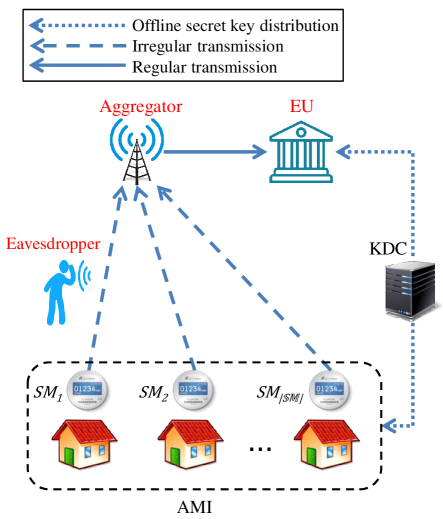
As shown in Fig. 1, our considered network model includes SMs, EU, aggregator, and an offline key distribution center (KDC). The role of each entity is described as follows.

• Key Distribution Center (KDC): It is responsible for generating and distributing the public and private keys of the cryptosystem used in our scheme. After key distribution, the KDC is not involved in the SMs’ readings collection process.

• Smart Meter (SM): A set of SMs, $\mathbb{SM}=\{SM_{i},1\leq i\leq|\mathbb{SM}|\}$, form an AMI network, where each $SM_{i}$ reports the real-time fine-grained power consumption reading if and only if there is an enough change in the power consumption comparing to the last reported reading, i.e., if the absolute value of the percentage of the change between the current consumption and the last reported reading exceeds a certain threshold. For instance, if the threshold is 5%, a reading is sent when the change in the consumption is above +5% or below -5%. Also, each $SM_{i}$ encrypts its power consumption reading and sends the ciphertext to a gateway, called the aggregator. In this case, the SMs may communicate directly with the gateway, or multi-hop data transmission is used to connect the SMs to the gateway, where some SMs may act as routers to relay other SMs’ readings.

• Aggregator: It acts as a local collector that aggregates all the received/stored encrypted power consumption readings sent by the SMs. Due to using the CAT approach, the aggregator stores the SMs’ power consumption readings to reuse the last reported readings for future reporting cycles in case that an SM does not report a power consumption reading. After collecting the encrypted SMs’ readings, the aggregator computes the ciphertext of the aggregated reading and forwards it to the EU without being able to reveal the individual readings or even the aggregated reading to preserve privacy.

• Electricity Utility (EU): The EU uses the fine-grained power consumption readings sent by SMs for load monitoring and energy management. It can use its decryption key to decrypt the ciphertext sent by the aggregator to obtain the total power consumption of the consumers of an AMI network while hiding the fine-gained power consumption reading of each consumer to preserve privacy.

Figure 1: Network Model.

III-B Threat Model

Threats may arise from either internal or external attackers. Internal attackers, which could be the SMs, the EU, or the aggregator, are assumed to be honest-but-curious. They follow the scheme honestly and do not disrupt the communication, but they are curious to infer whether the house dwellers are present at home or not by analyzing their transmission pattern. On the other hand, as shown in Fig. 1, an external adversary $\mathcal{A}$, e.g., eavesdropper, can intercept the wireless transmissions between the SMs and the aggregator over a period of time to create the transmission patterns of the consumers to launch PPA. This is because AMIs mostly use wireless communications [13, 8], and the broadcast nature of these communications can facilitate intercepting signals. Also, the attackers are assumed to have old absent/present records of the consumers’ transmission patterns that can be used to train a deep-learning model to launch PPA.

Basically, the objective of this paper is to preserve the privacy of the consumers’ activities by hiding the information that can be inferred from the consumers’ transmission patterns, i.e., no one including the EU and aggregator shall be able to learn the absence of the house dwellers. This complements the works in the literature that focus on preserving privacy by hiding the power consumption readings.

IV Preliminaries

In this section, we present a brief description of the cryptosystems and deep-learning approaches as well as the widely used activation functions that will be used in our scheme.

IV-A Bilinear Pairing

Let $\mathbb{G}$ and $\mathbb{G}_{T}$ be two cyclic groups of the same prime order $q$ and $P$ be a generator of group $\mathbb{G}$. Suppose $\mathbb{G}$ and $\mathbb{G}_{T}$ are equipped with a pairing, i.e., a non-degenerated and efficiently computable bilinear map $\hat{e}$: $\mathbb{G}\times\mathbb{G}\rightarrow\mathbb{G}_{T}$ such that:

• $\hat{e}(P,P)\neq 1_{\mathbb{G}_{T}}$

• $\hat{e}\left(aP_{1},bQ_{1}\right)=\hat{e}\left(P_{1},Q_{1}\right)^{ab}\in\mathbb{G}_{T}$, for all $a,b\in\mathbb{Z}_{q}^{*}$ and any $P_{1},Q_{1}\in\mathbb{G}$.

We will use bilinear pairing [22] to verify the SMs’ signatures efficiently.

Figure 2: Typical architecture of convolutional neural network (CNN).

IV-B Homomorphic Encryption

Homomorphic encryption is based on the Paillier cryptosystem that allows certain mathematical operations on the plaintext to be performed directly on the ciphertext [23]. Basically, the Paillier cryptosystem is comprised of three algorithms: key generation, encryption, and decryption.

• Key generation: To construct the public key, two large prime numbers $p_{1}$ and $q_{1}$ are first chosen, where $\left|p_{1}\right|=$ $\left|q_{1}\right|$, and then, $n$ and $\lambda$ are computed as follows: $n=p_{1}q_{1}$ and $\lambda=$ $\operatorname{lcm}\left(p_{1}-1,q_{1}-1\right)$. Next, ${\mu}$ is calculated as follows: ${\mu}=L(g^{\lambda}\bmod n^{2})^{-1}$ mod $n$, where $L(u)=$ $\frac{u-1}{n},$ and a generator $g\in\mathbb{Z}^{*}_{n^{2}}$. Hence, the public key is $pk=(n,g),$ and the corresponding private key is $sk=(\lambda,\mu)$.

• Encryption: Let $E(\cdot)$, $m\in\mathbb{Z}_{n},$ and $r\in\mathbb{Z}_{n}^{*}$ be the encryption function, a message, and a random number, respectively. The ciphertext can be calculated as follows.

  $$c=E(m)=g^{m}\cdot r^{n}\bmod n^{2}$$

• Decryption: Given the ciphertext $c\in\mathbb{Z}^{*}_{n^{2}}$, the plaintext is:

  $$m=D(c)=L\left(c^{\lambda\bmod n^{2}}\right)\cdot\mu\bmod n$$

  Then, the additive homomorphic property is as follows.

  $$E\left(m_{1}\right)\cdot E\left(m_{2}\right) =\left(g^{m_{1}}\cdot r_{1}^{n}\right)\left(g^{m_{2}}\cdot r_{2}^{n}\right)\bmod n^{2}$$

  $$=g^{m_{1}+m_{2}}\cdot\left(r_{1}r_{2}\right)^{n}\bmod n^{2}$$

  $$=E\left(m_{1}+m_{2}\right)$$

The homomorphic encryption is used in our scheme to aggregate the encrypted power consumption readings of the consumers in an AMI network without revealing the individual readings to preserve privacy.

IV-C Deep Learning

Deep learning is a special case of neural networks (NNs) in which multiple hidden layers are used. In general, the structure of NNs consists of three types of layers: input, output, and hidden [24]. There are two types of learning, including supervised and unsupervised learning. In supervised learning, a labeled dataset is used to train a model. Examples of such supervised learning approaches are the multi-layer perceptron (MLP) [25], convolutional neural network (CNN) [26], and recurrent neural network (RNN) [27]. Unsupervised learning, on the other hand, is used when the dataset is unlabeled. Clustering is the widely used approach in unsupervised learning to cluster unlabeled data with similar features together such as K-means clustering algorithm [28].

The training of a deep-learning model starts with feeding the features/input data into the model layers. Then, these features are gradually mapped into higher-level abstractions via the iterative update (a.k.a, feed-forward and back-propagation) through the intermediate layers of the model for a predefined number of iterations. These mapping abstractions can be used to determine the decision in the output layer. The model training involves learning the weight and the bias parameters $\Theta$ by defining a cost function and selecting an optimizer. Using the back-propagation algorithm [29], the model weights and biases are updated in each iteration using the gradients of the cost function. The output values of the model are compared to the correct values for optimizing the cost function. Then, the error is fed back through the layers to adjust the weights of each connection in order to reduce the cost (loss) function [29]. For the cost function in classification tasks, categorical cross-entropy $C(y,\hat{y})$ is defined to measure the loss due to the difference between the true distribution $y$ and the learned distribution $\hat{y}$, for $M$ classes as follows:

$$C(y,\hat{y})=\underset{\Theta}{\min}(-\sum_{c\,=\,1}^{M}y(c)\ log(\hat{y}(c))).$$

During training, an optimization method, e.g., Adam [30], is used for optimizing the cost function and labeled data are used to train the model. In addition, hyper-parameters of the model such as the number of neurons in each layer, the number of layers, and type of the optimizer, can be adjusted using k-fold cross validation, hyperopt [31], or any other validation methods [32].

In our scheme, we use CNN and gated recurrent unit neural network (GRU) to train the attacker and defense models, and use K-means clustering to label our dataset.

IV-D Convolutional Neural Network (CNN)

CNN is widely used in solving many challenging machine learning problems such as computer vision applications, natural language processing, and speech processing [26]. This wide adoption of CNN is due to its capability of capturing complex patterns in the input. In the following, we discuss the architecture of a CNN model.

As shown in Fig. 2, a typical architecture of a CNN model has input, convolution, pooling, fully connected, and output layers. A convolution layer consists of a set of independent filters and max pooling layer(s). The convolution operation is done by sliding each filter, which is usually small in size, over the input to extract features from the input. After the convolution step, a nonlinear activation function such as Rectified Linear Unit (ReLU), Sigmoid, or Tanh is used to enable the model to make complex decisions and solve difficult tasks. On the other hand, a pooling layer is used to compress the output of the convolution layer by sub-sampling the feature maps while retaining the most important information. Convolution and pooling layers are usually followed by one or more fully connected layers that process the features extracted to be used for inference.

IV-E Gated Recurrent Unit Neural Network (GRU)

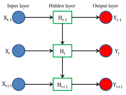
GRU is one type of RNNs that can memorize long sequences of input patterns by using hidden states, sometimes called hidden memory, and building connections between the internal units to form a directed graph as shown in Fig. 3 [33]. The key component in RNN is the transition function in each time step $t$ which takes the current time information $X_{t}$ and the previous hidden state ${H}_{t-1}$ and updates the current hidden state as follows.

$${H}_{t}={F}\left({X}_{t},{H}_{t-1}\right),$$ (1)

where ${F}$ is a nonlinear transformation/activation function, e.g., Sigmoid and Tanh functions. Due to the recurrent structure, ${H}_{t-1}$ in Eq. 1 can be regarded as a memory of previous inputs, i.e., RNN can remember previous inputs in the network’s internal state. In GRU, two gates are used, namely reset and update, to control the information flow and learn which information is important to keep and which information can be discarded. Hence, GRU has the ability to capture the correlations between the input, and that is why we will use it in training our models. GRU is usually used in the applications that need to predict the next word of a sentence based on the preceding words such as text generation [34]. It is also commonly used in speech recognition and synthesis [35].

IV-F K-means Clustering Technique

The K-means clustering technique is an unsupervised learning algorithm that is used to classify a given unlabeled dataset, which contains data objects/points, into a certain number of clusters based on the minimum distance between the cluster center and the object [28, 36]. A cluster is a collection of data objects that are homogeneous within the same cluster and heterogeneous to the objects in the other cluster(s) [36]. The main idea is to define $k$ centroids, one for each cluster, and each point in the dataset needs to be associated to the nearest centroid. Then, $k$ new centroids need to be re-calculated, and thus, new bindings have to be done between the same dataset points and the nearest new centroids. This process should be repeated several times, and in each time, the centriods’ locations are changed until convergence occurs when the centroids’ locations are not changed any more. This iterative process can be summarized in Fig. 4. Basically, the clustering algorithm aims at minimizing an objective function, e.g., a squared error function, as follows.

$$\mathrm{J}=\sum_{j=1}^{\mathrm{k}}\sum_{i=1}^{n}\left\|\mathrm{x}_{i}-\mathrm{c}_{\mathrm{j}}\right\|^{2},$$

where $\left\|\mathrm{x}_{i}-\mathrm{c}_{\mathrm{j}}\right\|^{2}$ is the Euclidean distance between a data point $\mathrm{x}_{i}$ and the cluster center $\mathrm{c}_{\mathrm{j}}$, for a given dataset of $n$ data points.

Figure 3: Typical architecture of deep recurrent neural network (RNN).

Figure 4: The flowchart of K-means clustering technique.

We will use K-means clustering technique to label the consumers’ records as “absent” and “present”, to be used in training our models.

IV-G Activation Functions

The activation functions are used in the machine learning models to transform the summed weighted input from a neuron into the activation of that neuron. They have a major impact on the model accuracy and convergence speed. In the following, we explain the widely used activation functions and their usage.

• Rectified Linear Unit (ReLU): It outputs the same input if the input is a positive value, otherwise, the output is zero [37]. ReLU is computationally efficient since it only requires a simple max() function as follows.

  $$ReLU(x)=max(0,x).$$

• Softmax: It is commonly used in the output layer for multi-class classification problems. For a given input vector, Softmax calculates a probability vector, i.e., for an input vector $\mathbf{z}=[\mathbf{z}[1],\ldots,\mathbf{z}[M]]\in\mathbb{R}^{M}$ of length $M$, where $M$ is the number of classes, the Softmax function is defined as follows [37].

  $$Softmax({z}[i])={\frac{e^{z[i]}}{\sum_{j=1}^{M}e^{z[j]}}}\ \ for\ \ i=\{1,\dots,M\}.$$

V Dataset Preparation

In this paper, we used a real smart meter dataset, which is available online and released by the Smart project [38]. The dataset contains real power consumption readings of $114$ single-family apartments over $349$ days during the year $2016$ from January $1^{st}$ to December $14^{th}$ at one-minute granularity. Hence, the total number of records is $39,786$, where each record corresponds to power consumption readings of one consumer in a single day. The dataset is then divided into two sets, 80% for training and 20% for testing. From the one-minute granularity (one reading/minute) dataset, we have created other datasets with different transmission rates, including a reading every 5 minutes, 15 minutes, and 30 minutes, by aggregating the power consumption readings. Note that we use “1/$x$ min” to refer to transmission rate, which means one reading is transmitted every $x$ minutes, where $x$ is the transmission interval. Using these datasets with thresholds of $1\%$, $4\%$, $7\%$, and $10\%$, we create datasets for CAT approach, in which an SM reports its power consumption reading if the absolute value of the percentage of the change in the consumption compared to the last reported reading exceeds the threshold.

Table I gives the efficiency that can be achieved by using CAT approach in terms of the percentage of readings that are not transmitted compared to periodic transmission of readings at different thresholds and transmission rates. We observe that as the threshold increases, the efficiency increases since the probability that the absolute value of the percentage of the change in the power consumption exceeds the threshold decreases, and hence, there are fewer transmissions. On the other hand, as the transmission interval increases, the efficiency decreases because the probability that the absolute value of the percentage of the change in the power consumption exceeds the threshold increases, and hence, there are more transmissions.

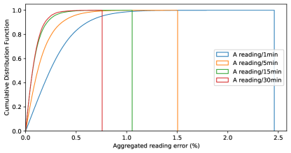
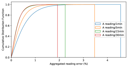
Using CAT approach, there may be a reading error because the reading that is considered by the EU may be less/more than the actual reading that is measured by the SM due to using a threshold. Therefore, the reading error at time $t$ is ($m_{SM}[t]-m_{EU}[t]$), where $m_{SM}[t]$ is the actual power consumption reading measured by the SM at time $t$ and $m_{EU}[t]$ is the reading that is used by the EU. Since the EU receives the aggregated reading of a number of SMs, we measured the error in the aggregated reading using our datasets assuming that the AMI network has $114$ SMs. Then, we plot, in Fig. 5, the cumulative distribution function (CDF) of the aggregated reading error at $5\%$ and $10\%$ thresholds using different transmission rates. It can be seen that the aggregated reading error in the worst case does not exceed half of the threshold, which indicates that the error in the aggregated reading is much smaller than the error of the individual readings because the positive errors in the individual readings counter the negative errors, which can reduce the aggregated reading error. Moreover, we observe that as the transmission interval increases, the error of the aggregated reading decreases because the probability that the absolute value of the percentage of the change in the power consumption exceeds the threshold increases, and hence, there are more transmissions which results in smaller error of the individual readings.

(a) Using $5\%$ threshold.

(b) Using $10\%$ threshold.

Figure 5: Comparison of CDF of aggregated reading error for different transmission rates at $5\%$ and $10\%$ thresholds.

TABLE I: Efficiency (%) achieved by using CAT approach at different thresholds and transmission rates.

		Threshold (%)
		$1$	$4$	$7$	$10$
	1/min	59.69	72.19	75.81	77.96
	1/5min	19.99	31.72	36.48	39.75
	1/15min	6.91	13.91	18.24	21.64
Transmission rate	1/30min	4.75	11.92	17.17	21.77

(a) Consumption pattern of consumer 1.

(b) Consumption pattern of consumer 2.

(c) Consumption pattern of consumer 3.

(d) Transmission pattern of consumer 1.

(e) Transmission pattern of consumer 2.

(f) Transmission pattern of consumer 3.

Figure 6: Consumption and transmission patterns of different consumers when they are present at home, where in (d)-(f), 1 and 0 refer to transmission and no transmission events, respectively.

(a) Consumption pattern of consumer 1.

(b) Consumption pattern of consumer 2.

(c) Consumption pattern of consumer 3.

(d) Transmission pattern of consumer 1.

(e) Transmission pattern of consumer 2.

(f) Transmission pattern of consumer 3.

Figure 7: Consumption and transmission patterns of different consumers when they are not at home, where in (d)-(f), 1 and 0 refer to transmission and no transmission events, respectively.

On the other hand, the existing power consumption datasets do not include the presence and absence of the consumers. Hence, in this section, we aim at labelling the consumers’ records per day as absent or present, to be used in training our models, by using the following two approaches.

1. Clustering: We used K-means clustering algorithm [28] for each consumer’s record to label it absent or present. The intuition behind using K-means clustering is that when the dwellers are not at home, their transmission pattern differs from the pattern when they are at home. So a clustering approach can classify the dataset records into two classes; one for “present” when the house dwellers are at home and “absent” when they are not at home. We clustered each consumer separately since each home has its own transmission pattern that depends on the lifestyle of its dwellers, the number of dwellers, etc.

2. Periods’ comparison: In this approach, we divide the day into three periods, $t_{1},t_{2},$ and $t_{3}$, that correspond to the following time periods, 8AM-4PM, 4PM-12AM, and 12AM-8AM, respectively. Then, if a consumer is present at home, the consumption at period $t_{2}$ is usually different from the consumption at this period because the consumer does many activities at the other periods such as cooking, as confirmed by [8]. First, we calculate the total consumption of each period $t_{i}$, where $i=\{1,2,3\}$, and then, we compute the following formula for each consumer’s record that has daily power consumption readings.

   $$\left|\dfrac{C_{1}[d]-C_{2}[d]}{C_{1}[d]}\right|+\left|\dfrac{C_{3}[d]-C_{2}[d]}{C_{3}[d]}\right|,$$

   where $C_{i}[d]$ is the total power consumption of the $i^{th}$ period in day $d$. The result of this formula is low when the consumption at periods $t_{1}$ and $t_{3}$ are close to the consumption at period $t_{2}$, which can indicate that the consumer is absent.

Finally, the records in our datasets are labelled absent if both approaches label them absent, otherwise they are labelled present.

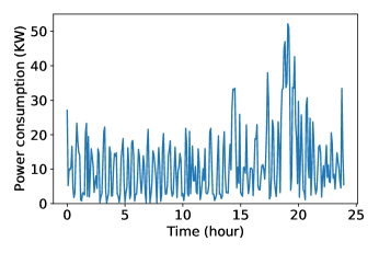
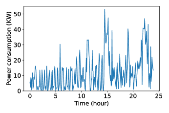
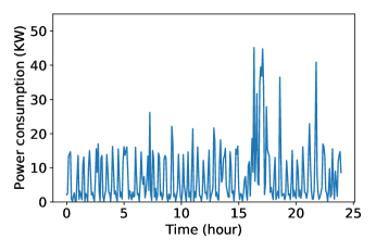
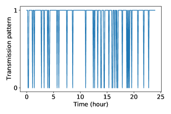
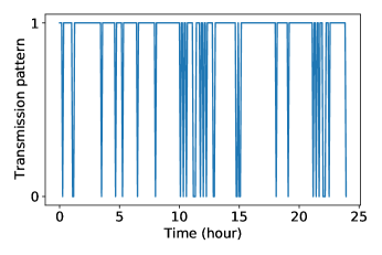
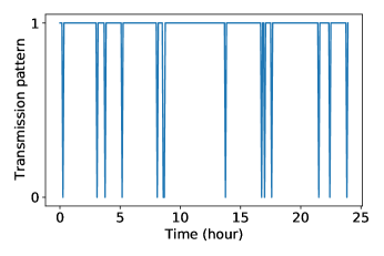
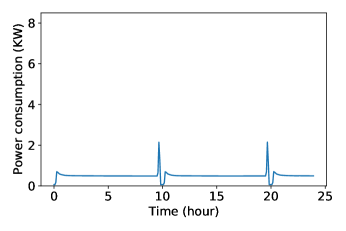
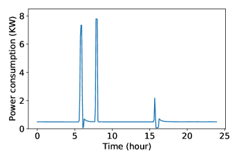
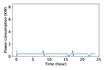
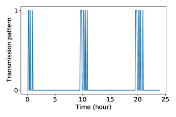
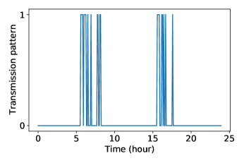
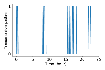
In this paper, we study two use cases at $10\%$ threshold; one using 1/5min (transmitting a reading every 5 minutes) and another using 1/30min (transmitting a reading every 30 minutes) transmission rates. Based on this threshold and transmission rates, we converted the datasets that have power consumption readings into datasets that have transmission patterns, containing zero or one in each time slot indicating no transmission event (when the absolute value of the percentage of the change in the consumption is below the threshold) or transmission event (when the absolute value of the percentage of the change in the consumption is above the threshold), respectively. Therefore, we have a transmission dataset that contains consumers’ records, where each record is labelled absent or present, and has $288$ and $48$ binary features, for 1/5min and 1/30min transmission rates, respectively. Fig. 6 and Fig. 7 show the power consumption and transmission patterns for three different consumers in our datasets when they are present at home and absent, respectively. As can be seen in the figures, there is a substantial difference in the transmission patterns based on the presence/absence of the consumers. Attackers can exploit this difference to use the transmission patterns to learn whether a consumer is present or absent. In next section, we will use this dataset for training and evaluating both the attacker and defense models.

VI Proposed scheme

In this section, we first use the dataset created in Section V to train an attacker model to launch PPA. The model takes the transmission pattern of a consumer as input and detects if the consumer is absent or present. Then, we train a deep-learning-based defense model that can generate spoofing transmissions (redundant real readings) to thwart PPA. Finally, we will discuss our privacy-preserving reading collection scheme.

VI-A Attacker Model

As explained in Section V, when a consumer is present at home, the transmission pattern is distinguishable due to using appliances comparing to the transmission pattern when the consumer is absent. In this subsection, we explain how attackers can make use of this fact by training a deep-learning model to launch PPA to learn whether a consumer is on travel (absent) or at home (present). The transmission pattern is the input of the model, and the output is either the house dwellers are present at home or absent.

VI-A1 Training the Attacker’s Model

A CNN-based model is used by the attacker to capture the temporal correlation in the input sequence. While training the attacker’s model, $\ell 2-$regularization is used to limit over-fitting. An overfitted model is a model that performs well on the training data and it does not perform well on new/unseen data. Also, we adjust the hyper-parameters of the CNN-based attacker model using hyperopt tool [31] on a validation dataset to tune the number of units in each layer, batch size, learning rate, and select an activation function for each layer. Moreover, Adam [30] optimizer is used to train the model for 60 epochs, 128 batch size, 0.001 learning rate, and categorical cross entropy as the loss function. To train the attacker’s model, we used Python3 libraries such as Scikit-learn [39], Numpy, TensorFlow [40], and Keras [41], which are installed on a high-performance cluster (HPC) of the Tennessee Tech University using a NVIDIA Tesla K80 GPU. The best performance of the attacker’s model can be achieved using the hyper-parameters given in Table II.

VI-A2 Attacker’s Deep-Learning Model Architecture

In the following, we present the detailed architecture of the attacker’s CNN-based model. 1-dimension CNN model (Conv1D) is used which consists of four convolution layers, an average pooling layer, four fully connected layers, and a softmax output layer. Table II gives the detailed structure of the attacker’s model in case of using 1/5min and 1/30min transmission rates including the number of layers, hidden units, and activation functions. The structure can be described as follows.

TABLE II: Attacker’s model architecture, where AF stands for activation function, and $h_{i}$ is the $i^{th}$ fully connected hidden layer.

	No. of units using		AF using
Layer	1/5min	1/30min	1/5min	1/30min
Input	288	48	Linear	Linear
Conv1D	150	80	ELu	ReLU
Conv1D	85	32	ReLU	ReLU
Conv1D	45	20	ReLU	ELu
Conv1D	25	–	ReLU	–
MaxPooling1D	2	2	–	–
$h_{1}$	512	256	ELu	ELu
$h_{2}$	512	512	ReLU	Sigmoid
$h_{3}$	128	64	Sigmoid	ELu
$h_{4}$	64	64	ELu	ReLU
Output	2	2	Softmax	Sigmoid

Figure 8: Illustration of the CNN-RNN-based defense architecture.

• The input layer is the first layer of the model, and it consists of nodes, called neurons. It receives the input data and passes them to the following layers. The number of neurons in the input layer is equal to the number of readings per day (or transmission pattern size), e.g., 288 readings per day if the transmission rate is one reading every 5 minutes.

• 1-dimension convolution layers are used to capture the temporal correlation in the input sequence using a number of convolution filters.

• A max pooling layer is used to combine the features extracted from the previous layer.

• Fully connected hidden layers are used to extract more features and make complex decisions.

• Softmax output layer is used to classify whether the dwellers are present or absent. Since we only have two classes, the output layer has two units.

VI-B Defense Model

The objective of this paper is to thwart transmission analysis attacks, including PPA, caused by using the CAT approach to preserve the consumers’ privacy while using their fine-grained power consumption readings for load monitoring and energy management. No one, including eavesdroppers, the utility, and the aggregator, should be able to learn whether the house dwellers are present at home or absent. The key challenge is how to send spoofing transmissions so that the attacker cannot distinguish between the transmission pattern generated by our defense model when a consumer is absent and the transmission pattern when the consumer is at home. The attacker should not also identify the spoofing transmissions because they are sent only when the consumer is absent. Therefore, in this subsection, we explain how the defense model is trained to generate spoofing transmissions using deep-learning to countermeasure PPA.

VI-B1 Dataset preparation for training the defense model

We used the generated dataset in Section V to create another dataset to train the defense model as follows. First, we create a sliding window of size $n$ elements and slide it on the transmission pattern of the consumer, so the new dataset contains $n$ elements from the transmission pattern and the label is the next element in the pattern. Note that each element in the transmission pattern is either one or zero in case there is a transmission or no transmission, respectively, in the corresponding time slot. In other words, the input of the defense model is a sequence of $n$ binary features, zeros and ones, and the label is the transmission decision in the next time slot, where one corresponds to transmit and zero corresponds to no transmit. By this way, our defense model acts as a predictor that takes $n$ elements from a transmission pattern and predicts next element. Since the model is trained on transmission patterns when the consumer is present at home, the model outputs an element that makes the pattern looks like the patterns generated when the consumer is present at home.

VI-B2 Defense model architecture

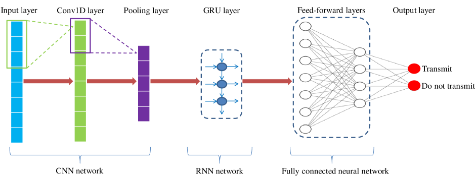
In the following, we present the detailed architecture of the defense model. As shown in Fig. 8, the defense model is a hybrid deep-learning model that combines a CNN with GRU followed by a fully connected neural network and a Softmax output layer. The input of the defense model is the transmission pattern of the last $n$ time slots and the output is the decision of either the SM needs to send a redundant power consumption reading (spoofing transmission) or not so that the generated transmission pattern looks like the patterns transmitted when the house dwellers are present at home. The same configuration, mentioned in Section VI-A1, that is used in training the attacker’s model, is also used in training the defense model, but with a batch size of 400 and the learning rate of 0.0001. The best performance of the defense model can be achieved using the hyper-parameters given in Table III.

The main reason of using a deep-learning model is that comparing with the traditional shallow learning methods such as logic regression, support vector machine, decision tree, etc., it can better capture the complex patterns within the data, which can improve the performance of the model. Moreover, the combination of CNN and GRU improves the extraction of the correlations between the previous transmission pattern and the current transmission decision, which is the key to improve the decision accuracy.

TABLE III: Defense model structure, where AF stands for activation function, and $h_{i}$ is the $i^{th}$ fully connected hidden layer.

	No. of units using		AF using
Layer	1/5min	1/30min	1/5min	1/30min
Input	100	35	Linear	Linear
Conv1D	150	128	ReLU	ReLU
Conv1D	–	64	–	ReLU
Conv1D	–	32	–	ReLU
MaxPooling1D	4	2	–	–
GRU	200	128	Tanh	Tanh
$h_{1}$	128	128	ReLU	ReLU
$h_{2}$	32	32	ReLU	ReLU
Output	2	2	Softmax	Softmax

Figure 9: An illustration of the defense methodology.

VI-B3 Defense methodology

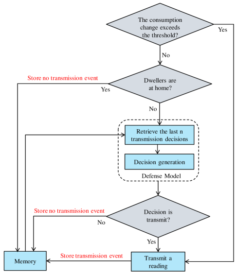
Fig. 9 shows the defense methodology that should be run in each time slot when the consumer is absent to decide whether a spoofing transmission (redundant reading) should be sent to defend against PPA. When the absolute value of the percentage of the change in the power consumption exceeds a threshold, regardless of the presence of dwellers, the SM should send the updated power consumption reading to the aggregator. On the other hand, when the dwellers are not at home, they run the defense model to decide whether the SM should transmit redundant readings to prevent the attacker from distinguishing the generated pattern by the defense model from the transmission patterns transmitted when the consumer is present at home to preserve the consumers’ privacy. A memory, as shown in Fig. 9, is used to store the transmission decision of each time slot, and it needs to keep only the last $n$ transmission decisions.

Our defense model works as follows. First, it retrieves the last $n$ transmission decisions from the SM’s memory and inputs them to the defense model, which is presented in Fig. 8. Then, the model outputs a decision which is either “transmit” or “do not transmit” a redundant power consumption reading (a spoofing transmission) as shown in Fig. 8. We have tried different values of $n$ and we found that the defense model gives good results at $n=100$ and $n=35$ in case of using 1/5min and 1/30min transmission rates, respectively.

VI-C Privacy-preserving Reading Collection Using CAT Approach

VI-C1 System Initialization

An offline KDC should bootstrap the system as follows. First, it generates the Paillier cryptosystem’s public key $(n=$ $pq,g),$ and the corresponding private key $(\lambda,\mu)$ where $p$ and $q$ are two large prime numbers with $|p|=|q|.$ Moreover, it generates the bilinear pairing parameters $\left(q_{1},\mathbb{G},\mathbb{G}_{T},P,\hat{e}\right)$. Furthermore, it chooses a secure hash function $H,$ where $H$: $\{0,1\}^{*}\rightarrow\mathbb{G}.$ Finally, it publishes the system parameters as $pubs=\left\{n,g,q_{1},\mathbb{G},\mathbb{G}_{T},P,\hat{e},H\right\}$. In addition, each $SM_{i}$ chooses a secret key $x_{i}\in\mathbb{Z}_{q}^{*}$, and computes the corresponding public key $Y_{i}=x_{i}P$. Similarly, the aggregator possesses private/public key pairs $x_{gw}/Y_{gw}$, respectively.

VI-C2 Reporting the Power Consumption Readings by SMs

When an $SM_{i}$ transmits a reading either due to a change in the consumption or a redundant reading (spoofing transmission) to preserve privacy, it encrypts the power consumption reading $m_{i}$ and sends it to the aggregator by performing the following steps.

• Step 1: $SM_{i}$ chooses a random number $r_{i}\in\mathbb{Z}_{n}^{*}$ and encrypts $m_{i}$ using Paillier cryptosystem as follows.

  $$C_{i}=g^{m_{i}}\cdot r_{i}^{n}\quad\bmod n^{2}$$

• Step 2: $SM_{i}$ uses its private key $x_{i}$ to generate a signature $\sigma_{i}$ as

  $$\sigma_{i}=x_{i}H\left(C_{i}\|TS\right),$$

  where $TS$ is a timestamp

• Step 3: $SM_{i}$ sends the following tuple to the aggregator.

  $$C_{i}\left\|TS\right\|\sigma_{i}$$

VI-C3 Aggregation by the Aggregator

The aggregator should store the last encrypted power consumption reading sent by each SM to reuse it in case that the SM does not send an encrypted reading because there is no enough change in the consumption. The aggregator should do the following steps to verify the SMs’ messages and calculate the ciphertext of the total aggregated reading of all SMs.

• Step $1$: Verification of the received messages: After receiving messages from the SMs, the aggregator first checks whether the timestamps are fresh or not. Then, it uses a batch verification approach to efficiently verify the received signatures instead of verifying the signatures individually as follows, where $w$ is the number of messages and $w\leq|\mathbb{SM}|$.

  $$\hat{e}\left(\sum_{i=1}^{w}\sigma_{i},P\right)\stackrel{{\scriptstyle?}}{{=}}\prod_{i=1}^{w}\hat{e}\left(H\left(C_{i}\|TS\right),Y_{i}\right)$$

  Proof of signature verification:
  

  $$\hat{e}\left(\sum_{i=1}^{w}\sigma_{i},P\right) \stackrel{{\scriptstyle}}{{=}}\prod_{i=1}^{w}\hat{e}\left(\sigma_{i},P\right)$$

  $$\stackrel{{\scriptstyle}}{{=}}\prod_{i=1}^{w}\hat{e}\left(x_{i}H\left(C_{i}\|TS\right),P\right)$$

  $$\stackrel{{\scriptstyle}}{{=}}\prod_{i=1}^{w}\hat{e}\left(H\left(C_{i}\|TS\right),x_{i}P\right)$$

  $$\stackrel{{\scriptstyle}}{{=}}\prod_{i=1}^{w}\hat{e}\left(H\left(C_{i}\|TS\right),Y_{i}\right).$$

• Step $2$: Privacy-preserving readings aggregation: The aggregator should compute the encrypted aggregated fine-grained reading $C_{gw}$ as follows.

  $$C_{gw}=\prod_{i=1}^{|\mathbb{SM}|}C_{i}\quad\bmod n^{2}$$

• Step $3$: The aggregator uses its private key $x_{gw}$ to compute the signature as follows.

  $$\sigma_{gw}=x_{gw}H\left(C_{gw}\|TS\right)$$

• Step $4$: The aggregator composes a message containing the encrypted aggregated reading and a signature and sends it to the EU. The message should have the following tuple.

  $$C_{gw}\|TS\|\sigma_{gw}$$

VI-C4 Aggregated Reading Recovery by the EU

Upon receiving the message from the aggregator, the EU checks the freshness of the timestamp and verifies the signature by checking the following.

$$\hat{e}\left(\sigma_{gw},P\right)\stackrel{{\scriptstyle?}}{{=}}\hat{e}\left(H\left(C_{gw}\|TS\right),Y_{gw}\right)$$

Proof of signature verification:

$$\hat{e}(\sigma_{gw},P) \stackrel{{\scriptstyle}}{{=}}\hat{e}(x_{gw}H(C_{gw}\|TS),P)$$

$$\stackrel{{\scriptstyle}}{{=}}\hat{e}(H(C_{gw}\|TS),x_{gw}P)$$

$$\stackrel{{\scriptstyle}}{{=}}\hat{e}\left(H\left(C_{gw}\|TS\right),Y_{gw}\right).$$

Then, the EU uses the secret key $(\lambda,\mu)$ to decrypt $C_{gw}$, and recover the total power consumption reading of the SMs $R_{T}$ as follows.

$$R_{T}=D\left(C_{gw}\right)=L\left(C_{gw}^{\lambda}\bmod n^{2}\right)\cdot\mu\bmod n=\sum_{i=1}^{|\mathbb{SM}|}m_{i}$$

VII Evaluations

In this section, we first discuss the performance metrics and then evaluate the attacker’s success rate in determining the absence of the house dwellers by analyzing the transmission pattern without using our defense. Next, we evaluate the success of the attacker while using our defense model assuming that the attacker does not know the defense model. Finally, we evaluate the attacker’s success assuming that the attacker knows the defense model.

VII-A Performance Metrics

In order to evaluate our models’ performance, we consider the following metrics. The success rate ($SR$) is the probability that the attacker successfully detects that the house dwellers are not at home (absent). The false alarm rate ($FA$) is the probability that the attacker thinks that the dwellers are absent but they are actually present at home. The defense model performance is better when $SR$ is low. These metrics are measured as follows.

$$\small\textrm{$SR$}=\frac{\textrm{$TP$}}{\textrm{$TP$}+\textrm{$FP$}},\quad\textrm{$FA$}=\frac{\textrm{$FP$}}{\textrm{$TN$}+\textrm{$FN$}},$$

where, $TP$, $TN$, $FN$, and $FP$ stand for true positive, true negative, false negative, and false positive, respectively. Moreover, we measure also the efficiency of the CAT approach with and without our defense in terms of the percentage of readings that are not transmitted, which is related to the saving in the communication bandwidth, compared to continuous transmission approach. The efficiency is computed as follows.

$$\small\textrm{Efficiency (\%)}=\frac{\textrm{$P_{t}$}-\textrm{$R_{t}$}}{\textrm{$P_{t}$}}\times 100,$$

where $P_{t}$ is the number of readings that are sent when SMs send the readings continuously (without using CAT approach) and $R_{t}$ is the number of readings sent by our scheme that uses the CAT approach.

VII-B Attacker’s Success Rate Without Our Scheme

As mentioned in Section III-B, the attacker has old absent/present records of the transmission patterns of the consumers. These records are used to train a deep-learning model, which is discussed in Section VI-A, to infer the absence of house dwellers by running the model using the consumer’s transmission pattern. Using this model and without using our defense model, the attacker’s success rates are 91.1% and 88.5% in case of 1/5min and 1/30min transmission rates, respectively, as can be seen in Table IV. The reduction in the success rate with the increasing of the transmission interval is because as the transmission interval increases, the number of transmissions decreases, which results in hiding detailed information from the consumption pattern. From the given results, we can conclude that the attacker can infer the absence of the dwellers with high confidence.

VII-C Attacker’s Success Rate With Our Scheme if the Defense Model is Unknown

In this subsection, we evaluate the performance of our defense model assuming that the attacker does not know the defense model. The attacker uses the transmission patterns generated by our defense model as input to the attacker model, discussed in Section VI-A, to know whether the house dwellers are absent. As shown in Table IV, the attacker’s success rate is significantly reduced from 91.1%, without using our defense model, to only 3.15% using our defense with 1/5min transmission rate, while the attacker’s success rate is reduced from 88.5% to 2.25% with 1/30min transmission rate. This big reduction in the success rate of the attacker indicates that our defense model can generate patterns that look like the patterns transmitted when the consumer is at home, and that is why the attacker’s model was not able to classify the patterns generated by our defense model as absent.

Moreover, using 1/5min transmission rate at $10\%$ threshold, our scheme can achieve efficiency of 40.8% compared to 69.67% in case that privacy is not preserved. Also, using 1/30min transmission rate, the efficiency is reduced from 44.6% to 19.01% using our defense, as shown in Table IV. This reduction in efficiency is due to sending redundant readings to preserve privacy, and this can be considered the cost for privacy preservation. Note that better efficiency can be achieved by reducing the number of redundant readings but with higher attacker’s success, i.e., there is a trade off between the efficiency and attacker’s success rate. From our experiment results, we can see that the less the transmission rate (longer transmission interval), the more reduction in efficiency since the likelihood that the power consumption change exceeds the threshold increases which causes more transmissions.

TABLE IV: Evaluations with and without our defense model for 1/5min and 1/30min transmission rates at $10\%$ threshold.

Transmission rate	1/5min	1/30min
Attacker’s success rate without our scheme	91.1%	88.5%
Attacker’s success rate with our scheme	3.15%	2.25%
Efficiency without our scheme	69.67%	44.6%
Efficiency with our scheme	40.8%	19.01%

VII-D Attacker’s Success With Our Scheme if the Defense Model is Known

In this subsection, we evaluate the performance of our scheme when the attacker knows the defense model. In Sections VII-B and VII-C, we assume that the attacker has old absent/present records of the transmission patterns of the consumers, and using these records, the attacker trained a deep-learning model to learn whether a consumer is absent. In this subsection, we assume a stronger attacker who knows not only old transmission patterns but also the defense model. Using the available knowledge to the attacker, he can launch powerful attacks as follows. First, the attacker uses the absent records and the defense model to create “spoofing” patterns. Then, using absent, present, and spoofing patterns, the attacker trains an advanced model to classify the input patterns into “absent”, “present”, or “spoofing”. Hence, if the classification is “spoofing”, the attacker thinks that the victim consumer is absent and the defense model is used to generate patterns with spoofing transmissions.

The best performance of the attacker’s model, when the defense model is known in case of using 1/5min and 1/30min transmission rates, can be achieved using the hyper-parameters given in Table V. By knowing the defense model by the attacker, the success rate of detecting the absence of the house dwellers increases from 3.15% to 13.52% and from 2.25% to 12.84% using 1/5min and 1/30min transmission rates, respectively. These results are good given the strong assumptions that the attacker knows the defense model and has old transmission patterns.

TABLE V: Attacker’s model architecture when the defense model is known to the attacker, where AF stands for activation function, and $h_{i}$ is the $i^{th}$ fully connected hidden layer.

	No. of units using		AF using
Layer	1/5min	1/30min	1/5min	1/30min
Input	288	48	Linear	Linear
Conv1D	150	128	ReLU	ReLU
MaxPooling1D	4	4	–	–
GRU	–	32	–	Tanh
$h_{1}$	128	64	ReLU	ReLU
$h_{2}$	35	32	ReLU	ReLU
Output	3	3	Softmax	Softmax

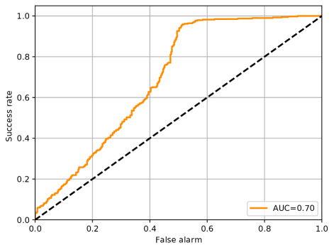
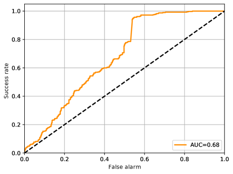
In addition, Figs. 10 and 11 show the Receiver Operating Characteristic (ROC) curves of the attacker model in case of 1/5min and 1/30min transmission rates, respectively, assuming that the defense model is known. ROC curve is often used to evaluate the classification accuracy, which is measured by the area under the curve (AUC). This area indicates how the model can distinguish between the classes, where a bigger AUC indicates a better performance. We assume that a false alarm rate of 0.05 is acceptable to the attacker, and then, we need to determine the success rate at this false alarm rate. As can be seen in Figs. 10 and 11, at false alarm of 0.05, the attacker’s success rate is fairly low (less than 0.1) compared to more than 0.6 using ASP proposed in [8]. Therefore, the attacker can detect the absence of the house dwellers with a high probability in ASP [8], while the success rate in our scheme is much lower. This is because our scheme is trained on the transmission patterns when the consumer is present at home, and then it uses spoofing transmissions (redundant real readings) when the consumer is absent to generate a pattern that looks similar to the consumer’s transmission patterns when he/she is at home.

Figure 10: The ROC curve of the attacker model when the defense model is known using 1/5min transmission rate at $10\%$ threshold.

Figure 11: The ROC curve of the attacker model when the defense model is known using 1/30min transmission rate at $10\%$ threshold.

VII-E Discussions

In this paper, we consider a strong attack model assuming that the attacker has old transmission patterns and knows the defense model. Using this knowledge, the attacker trains a sophisticated deep-learning model to detect the absence of the house dwellers. On the other hand, the design of our defense scheme is based on a deep-learning model which is trained on the transmission patterns when the consumers are present at home to generate spoofing transmissions so that the attacker cannot distinguish the pattern generated using STDL from the patterns transmitted when the consumers are at home to preserve consumers’ privacy. The scheme in [8] is customized, i.e., the scheme depends on the distribution of the power consumption changes (transmission patterns) of each consumer, but our model is general (one model for all consumers) and it can be applied to new consumers who have no old transmission patterns. Furthermore, we assume that the network nodes, including the SMs, EU, and aggregator, are honest but curious, while the scheme in [8] assumes that they are trusted and the defense is limited only to the eavesdroppers.

Moreover, our scheme can achieve the following desirable privacy requirements that can counter the attacks mentioned in Section III-B.

PPA countermeasure: An adversary can eavesdrop on the wireless transmissions between the SMs and the aggregator and construct the transmission patterns of the consumers, and then launch PPA. On the other hand, the aggregator and EU are curious to learn whether the house dwellers are absent by analyzing their SMs’ transmission patterns. However, using our scheme, no one can learn whether the house dwellers are absent because it sends spoofing transmissions (redundant real readings) to make it difficult for the attacker to learn this information.

Consumers’ fine-grained readings’ privacy preservation: To ensure the privacy of the consumers, each SM first encrypts its readings using the public key of the Paillier cryptosystem and no entity is able to learn the individual readings to preserve consumers’ privacy. In addition, if the same reading is repeated at different times, the ciphertext looks different because the encryption uses a one-time random number. Also, when an SM sends a redundant reading that is similar to the last reported reading to preserve privacy, the ciphertext looks different and the aggregator cannot know that the reading is redundant. This is important to prevent the aggregator and eavesdroppers from identifying redundant readings (spoofing transmissions) because these readings are sent only when the house dwellers are absent. It is important to use the random number $r$ once because if it is reused, the difference between two readings, i.e., $m_{1}$ and $m_{2}$, can be obtained by dividing their ciphertexts $g^{m_{1}}\cdot r^{n}/g^{m_{2}}\cdot r^{n}=g^{m_{1}-m_{2}}$, and this can be solved to obtain ${m_{1}-m_{2}}$; hence, by knowing one reading, the other one can be obtained.

Confidentiality of AMI’s total power consumption: The aggragator should send the ciphertext of the AMI’s total power consumption to the EU for load monitoring, after computing it from the encrypted fine-grained power consumption readings of the SMs. The aggregator and the attackers, who eavesdrop on the communications between the aggregator and the EU learn nothing about the total consumption of an AMI since the private key which is known only to the EU is needed for decrypting Paillier ciphertext to obtain the aggregated power consumption reading.

VIII Conclusion

In this paper, we have proposed STDL, an efficient and privacy-preserving scheme for collecting power consumption readings in AMI networks. Our scheme is efficient because the SMs do not send the readings if there is no enough change in the power consumption comparing to the last report reading. It also preserves the consumers’ privacy by transmitting redundant readings (spoofing transmissions) using a deep-learning-based defense scheme. First, a real dataset for power consumption readings dataset and clustering technique are used to create a dataset for transmission patterns using CAT approach. Then, we train an attacker model using deep-learning, and our evaluations indicate that the attacker’s success rate is about 91%. Next, we train a deep-learning-based defense scheme to send spoofing transmissions efficiently to thwart PPA attacks. Extensive evaluations are conducted, and the results indicate that our scheme can reduce the attacker’s success rate to 13.52% in case he knows the defense model and to 3.15% in case he does not know the model, while still achieving high efficiency in terms of the number of readings that should be transmitted. This big reduction in the attacker’s success rate indicates that our defense can generate patterns that look like the patterns transmitted when the consumer is at home. Moreover, our measurements indicate that the proposed scheme can reduce the number of readings that should be transmitted by about 41% while preserving the privacy of the consumers.

References

- [1] V. C. Gungor, D. Sahin, T. Kocak, S. Ergut, C. Buccella, C. Cecati, and G. P. Hancke, “A survey on smart grid potential applications and communication requirements,” IEEE Transactions on Industrial Informatics, vol. 9, no. 1, pp. 28–42, Feb. 2013.
- [2] Z. M. Fadlullah, M. M. Fouda, N. Kato, A. Takeuchi, N. Iwasaki, and Y. Nozaki, “Toward intelligent machine-to-machine communications in smart grid,” IEEE Communications Magazine, vol. 49, no. 4, pp. 60–65, Apr. 2011.
- [3] C. Efthymiou and G. Kalogridis, “Smart grid privacy via anonymization of smart metering data,” Proc. of IEEE international conference on smart grid communications, pp. 238–243, Oct. 2010.
- [4] G. W. Hart, “Nonintrusive appliance load monitoring,” Proceedings of the IEEE, vol. 80, no. 12, pp. 1870–1891, 1992.
- [5] H. Mohammed, S. Tonyali, K. Rabieh, M. Mahmoud, and K. Akkaya, “Efficient privacy-preserving data collection scheme for smart grid AMI networks,” Proc. of IEEE Global Communications Conference (GLOBECOM), pp. 1–6, Dec. 2016.
- [6] M. I. Ibrahem, M. M. Badr, M. M. Fouda, M. Mahmoud, W. Alasmary, and Z. M. Fadlullah, “PMBFE: Efficient and privacy-preserving monitoring and billing using functional encryption for AMI networks,” Proc. of IEEE International Symposium on Networks, Computers and Communications (ISNCC’20), Montreal, Canada, Oct. 2020.
- [7] M. I. Ibrahem, M. Nabil, M. M. Fouda, M. Mahmoud, W. Alasmary, and F. Alsolami, “Efficient privacy-preserving electricity theft detection with dynamic billing and load monitoring for AMI networks,” IEEE Internet of Things Journal, 2020, doi: 10.1109/JIOT.2020.3026692.
- [8] H. Li, S. Gong, L. Lai, Z. Han, R. C. Qiu, and D. Yang, “Efficient and secure wireless communications for advanced metering infrastructure in smart grids,” IEEE Transactions on Smart Grid, vol. 3, no. 3, pp. 1540–1551, Sep. 2012.
- [9] M. A. Lisovich, D. K. Mulligan, and S. B. Wicker, “Inferring personal information from demand-response systems,” IEEE Security Privacy, vol. 8, no. 1, pp. 11–20, Feb. 2010.
- [10] S. Finster and I. Baumgart, “Privacy-aware smart metering: A survey,” IEEE Communications Surveys Tutorials, vol. 17, no. 2, pp. 1088–1101, Apr. 2015.
- [11] K. Weaver, “A perspective on how smart meters invade individual privacy,” Last accessed: Nov. 2020. [Online]. Available: https://skyvisionsolutions.files.wordpress.com/2014/08/utility-smart-meters-invade-privacy-22-aug-2014.pdf
- [12] S. Yussof, M. E. Rusli, Y. Yusoff, R. Ismail, and A. A. Ghapar, “Financial impacts of smart meter security and privacy breach,” Proc. of International Conference on Information Technology and Multimedia, pp. 11–14, Nov. 2014.
- [13] M. Alam, M. Reaz, and M. Ali, “A review of smart homes—past, present, and future,” IEEE Transactions on Systems, Man, and Cybernetics, Part C (Applications and Reviews), vol. 42, no. 6, pp. 1190–1203, Nov. 2012.
- [14] K. Samarakoon, J. Ekanayake, and N. Jenkins, “Reporting available demand response,” IEEE Transactions on Smart Grid, vol. 4, no. 4, pp. 1842–1851, Dec. 2013.
- [15] K. Carrie Armel, A. Gupta, G. Shrimali, and A. Albert, “Is disaggregation the holy grail of energy efficiency? the case of electricity,” Energy Policy, vol. 52, pp. 213 – 234, Jan. 2013.
- [16] S. Werner and J. Lunden, “Event-triggered real-time metering in smart grids,” Proc. of European Signal Processing Conference (EUSIPCO), pp. 2701–2705, Sep. 2015.
- [17] S. Werner and J. Lundén, “Smart load tracking and reporting for real-time metering in electric power grids,” IEEE Transactions on Smart Grid, vol. 7, no. 3, pp. 1723–1731, May. 2016.
- [18] J. Lunden and S. Werner, “Real-time smart metering with reduced communication and bounded error,” Proc. of IEEE International Conference on Smart Grid Communications (SmartGridComm), pp. 326–331, Nov. 2014.
- [19] M. Simonov, G. Chicco, and G. Zanetto, “Event-driven energy metering: Principles and applications,” IEEE Transactions on Industry Applications, vol. 53, no. 4, pp. 3217–3227, Aug. 2017.
- [20] A. Proano, L. Lazos, and M. Krunz, “Traffic decorrelation techniques for countering a global eavesdropper in WSNs,” IEEE Transactions on Mobile Computing, vol. 16, no. 3, pp. 857–871, Mar. 2017.
- [21] S. Alsemairi and M. Younis, “Adaptive packet-combining to counter traffic analysis in wireless sensor networks,” Proc. of International Wireless Communications and Mobile Computing Conference (IWCMC), pp. 337–342, Aug. 2015.
- [22] D. Boneh and M. Franklin, “Identity-based encryption from the weil pairing,” Advances in Cryptology — CRYPTO 2001, pp. 213 – 229, 2001.
- [23] P. Paillier, “Public-key cryptosystems based on composite degree residuosity classes,” Proc. of international conference on the theory and applications of cryptographic techniques, pp. 223–238, Apr. 1999.
- [24] Z. Zheng, Y. Yang, X. Niu, H. Dai, and Y. Zhou, “Wide and deep convolutional neural networks for electricity-theft detection to secure smart grids,” IEEE Transactions on Industrial Informatics, vol. 14, no. 4, pp. 1606–1615, Apr. 2018.
- [25] S. Haykin, Neural Networks and Learning Machines: A Comprehensive Foundation (3rd Edition). USA: Prentice-Hall, Inc., Nov. 2008.
- [26] Y. LeCun et al., “Convolutional networks for images, speech, and time series,” The handbook of brain theory and neural networks, vol. 3361, no. 10, pp. 255–258, 1995.
- [27] D. Ha and J. Schmidhuber, “Recurrent world models facilitate policy evolution,” in Advances in Neural Information Processing Systems, pp. 2450–2462, 2018.
- [28] K. M. Faraoun and A. Boukelif, “Neural networks learning improvement using the k-means clustering algorithm to detect network intrusions,” International Journal of Computer and Information Engineering, vol. 1, no. 10, pp. 3151 – 3158, 2007.
- [29] S. Chaturvedi, R. N. Titre, and N. Sondhiya, “Review of handwritten pattern recognition of digits and special characters using feed forward neural network and Izhikevich neural model,” Proc. of International Conference on Electronic Systems, Signal Processing and Computing Technologies, pp. 425–428, Jan. 2014.
- [30] D. P. Kingma and J. Ba, “Adam: A method for stochastic optimization,” Proc. of International Conference on Learning Representations, San Diego, CA, USA, May. 2015.
- [31] J. Bergstra, B. Komer, C. Eliasmith, D. Yamins, and D. D. Cox, “Hyperopt: a Python library for model selection and hyperparameter optimization,” Computational Science & Discovery, doi: https://doi.org/10.1088/1749-4699/8/1/014008, 2015.
- [32] M. Nabil, M. Ismail, M. Mahmoud, M. Shahin, K. Qaraqe, and E. Serpedin, “Deep recurrent electricity theft detection in AMI networks with random tuning of hyper-parameters,” Proc. of International Conference on Pattern Recognition (ICPR), pp. 740–745, Aug 2018.
- [33] W. Yin, K. Kann, M. Yu, and H. Schütze, “Comparative study of CNN and RNN for natural language processing,” arXiv preprint arXiv:1702.01923, 2017.
- [34] A. F. Ganai and F. Khursheed, “Predicting next word using RNN and LSTM cells: Stastical language modeling,” Proc. of International Conference on Image Information Processing (ICIIP), pp. 469–474, Nov. 2019.
- [35] A. Graves, A. Mohamed, and G. Hinton, “Speech recognition with deep recurrent neural networks,” Proc. of IEEE International Conference on Acoustics, Speech and Signal Processing, pp. 6645–6649, May. 2013.
- [36] B. Dash, D. Mishra, A. Rath, and M. Acharya, “A hybridized k-means clustering approach for high dimensional dataset,” International Journal of Engineering, Science and Technology, vol. 2, no. 2, pp. 59–66, 2010.
- [37] C. Nwankpa, W. Ijomah, A. Gachagan, and S. Marshall, “Activation functions: Comparison of trends in practice and research for deep learning,” arXiv preprint arXiv:1811.03378, 2018.
- [38] Kolter, “Residential Energy Disaggregation Dataset (REDD),” Last accessed: 2020. [Online]. Available: http://traces.cs.umass.edu/index.php/Smart/Smart
- [39] F. Pedregosa et al., “Scikit-learn: Machine learning in Python,” Journal of Machine Learning Research, vol. 12, pp. 2825–2830, Oct. 2011.
- [40] A. Martín et al., “TensorFlow: Large-scale machine learning on heterogeneous systems,” 2015, software available from tensorflow.org. [Online]. Available: https://www.tensorflow.org/
- [41] F. Chollet et al., “Keras,” https://github.com/fchollet/keras, 2015.