Enhancement by postfiltering for speech and audio coding in ad-hoc sensor networks

Abstract

Enhancement algorithms for wireless acoustics sensor networks (WASNs) are indispensable with the increasing availability and usage of connected devices with microphones. Conventional spatial filtering approaches for enhancement in WASNs approximate quantization noise with an additive Gaussian distribution, which limits performance due to the non-linear nature of quantization noise at lower bitrates. In this work, we propose a postfilter for enhancement based on Bayesian statistics to obtain a multidevice signal estimate, which explicitly models the quantization noise. Our experiments using PSNR, PESQ and MUSHRA scores demonstrate that the proposed postfilter can be used to enhance signal quality in ad-hoc sensor networks.

1 Introduction

The emergence of connected and portable devices like smartphones, and the rising popularity of voice user-interfaces and devices equipped with microphones, enable the necessary infrastructure for ad-hoc wireless acoustic sensor networks (WASNs). The dense, ad-hoc positioning and collaboration in a WASN leads to efficient sampling of the acoustic space, thereby gaining higher quality signal estimates compared to single-channel estimates [1]. Typical applications of ad-hoc WASNs use microphones on low-resource devices, such that we need low-complexity methods and which use bandwidth efficiently to compress and transmit the acoustic signals. This involves quantization at the encoder, whereby the received signal at the decoder is usually degraded by quantization noise [2, 3, 4, 5, 6].

Past works on WASN often overlook the variability in maximum capacity of sensors [7]. However, rate-constrained spatial filtering like beamforming and multichannel Wiener filtering have been used in binaural hearing aids (HAs) [8, 9, 10, 11, 3]. A study on rate-constrained optimal beamforming showed the advantage of using spatially separated microphones in HAs, although the method assumes that the joint statistics of signals are available at the processing nodes [8]. Subsequently, sub-optimal strategies for noise reduction which do not use the joint statistics at the nodes have been proposed [8, 9, 10, 11, 12]. While the above methods are effective in reducing noise, they are either limited to, or are most efficient with two nodes (HAs) only. In a recent work on multi-node WASN, a linearly-constrained minimum variance beamformer was used to optimize rate allocation and sensor selection over nodes, based on spatial location and frequency content [13, 14]. However, due to the dynamic nature of an ad-hoc WASN, information about sensor distribution, location, number of target and interference sources may be either unavailable, or their exchange between nodes further adds to the bandwidth consumption and communication complexity. Further, the above methods assume an additive quantization noise model, which is accurate only at higher bitrates. Lastly, while all the above methods are optimized on Wyner-Ziv coding, their suitability in combination with existing speech and audio coding has not been demonstrated yet. Their performance in single-channel mode can therefore not compete with conventional single-channel codecs.

Figure 1: Distribution of microphones in the ad-hoc acoustic sensor network.

In this paper, we propose a Bayesian postfilter for enhancement in ad-hoc WASNs, which explicitly models the quantization noise within the optimization framework of the filter, and can be applied on top of existing codecs with minimal modifications. Thus, the main contribution of the current work is the postfilter which takes quantization into account through truncation, while retaining the conventional assumption of additive Gaussian background noise, thereby resulting in a truncated Gaussian representation of the clean speech distribution. To evaluate the proposed methodology, we place the necessary assumptions that the devices are dominantly degraded by either background noise and reverberation, or coding noise due to quantization, and each device operates at its maximum capacity. In line with past works, we show that by distributing the total available bitrate between the two sensors, the output gain of the WASN signal estimate is higher than the output gain of a low input-SNR single sensor transmitting at full bitrate [8, 9, 10, 11]. In addition, we present the advantages of incorporating the exact quantization noise models within the optimization framework. In order to focus on the effect of the postfilter on quantization noise, we apply the proposed method on the output of a codec [15], which is specifically designed to address multi-device coding. To the best of our knowledge, this is the first time a complete WASN system is evaluated with competitive performance also in a single-channel codec mode. Although we have not yet included models of spatial configuration of sensors, room impulse responses or multiple sources, we show that the proposed method already yields large output gains.

2 Methodology

To focus on the novel aspects of the approach, we consider a simple WASN consisting of two devices with microphones: 1. a low-resource device A with high input SNR and 2. a high-resource device B with low input SNR, as illustrated in Fig. 1. An example application is a smartwatch that collaborates with a distant smart speaker. Let $x(k,t),n(k,t)$ be the perceptual domain representations of the speech and noise signal, respectively, at the frequency bin $k$ and time frame $t$ [16]; the perceptual domain representations are computed by dividing the frequency domain signals by the perceptual envelope obtained from the codec [16]. These signals can be approximated by zero-mean Gaussian distributions with variances $\sigma_{x}^{2}$ and $\sigma_{n}^{2}$, whereby the random variables are correspondingly $X\sim\mathcal{N}(0,\sigma_{x}^{2}),\quad N\sim\mathcal{N}(0,\sigma_{n}^{2})$ [17]. Under the assumption of uncorrelated, additive background noise, the noisy signal $y(k,t)=x(k,t)+n(k,t)$ is Gaussian distributed with $Y\sim\mathcal{N}(0,\sigma_{y}^{2})$, and variance $\sigma_{y}^{2}=\sigma_{x}^{2}+\sigma_{n}^{2}$ [17]. Our goal is to estimate the distribution of clean speech, conditioned over the noisy observation $P(X\mid Y)$, in other words, the posterior distribution [18]. We obtain estimates for every time-frequency bin, and shall omit the time and frequency subscripts in the rest of the section to aid readability. According to the Bayes rule, the posterior distribution can be written as:

$$P(X\mid Y)=\frac{P(X)P(Y\mid X)}{P(Y)}\propto P(X)P(Y\mid X),$$ (1)

where $P(X)$ and $P(Y)$ are the prior distributions of the speech and observed signals and $P(Y\mid X)$ is the conditional likelihood. However, our quantized observation, $y_{q}(k,t)$ of the noisy signal gives more evidence about $X$; The true value of the noisy signal $Y$ lies within the quantization bin limits, $y(k,t)\in[l(k,t),u(k,t)]$ and the lower and upper bin limits for the quantization levels in a frame $\{\mathbf{l},\mathbf{u}\}\in\mathbb{R}^{K\times 1}$ are obtained from the observed quantized spectrum of a frame $\mathbf{y}_{q}\in\mathbb{R}^{K\times 1}$ [19]. Since the true noisy signal lies in the bounded field $l(k,t)\leq Y\leq u(k,t)$, we compute the summation of the likelihood over the quantization bin limits to obtain the posterior distribution of speech,

$$P(X)_{(l\leq Y\leq u)}\propto P(X)\int_{l}^{u}P(Y\mid X)dy,$$ (2)

where $\propto$ signifies equality up to a scaling factor. Eq. 2 can be rewritten as the difference between cumulative distributions, $P(X)_{(l\leq Y\leq u)}\propto P(X)(F(u)-F(l))$. The conditional likelihood can be represented as $P(Y\mid X)\sim\mathcal{N}(x,\sigma_{n}^{2})$, thus resulting in the final equation for the posterior distribution,

$$P(X)_{(l\leq Y\leq u)}\propto P(X)\left[0.5\bigg{\{}\operatorname{erf}\left(\frac{u-x}{\sigma_{n}\sqrt{2}}\right)-\operatorname{erf}\left(\frac{l-x}{\sigma_{n}\sqrt{2}}\right)\bigg{\}}\right],$$ (3)

where $\operatorname{erf}(.)$ is the error function. Note that due to the use of the exact quantization bin limits, $P(X)_{(l\leq Y\leq u)}$ corresponds to a truncated Gaussian [20]. This is in contrast to past works, where the quantization noise is approximated by an additive Gaussian distribution, which is an accurate approximation only at high bitrates [13].

Figure 2: Block diagrams showing (a) the overall system structure with the location of the postfilter, and (b) overview of the postfilter.

From Eq. 3, the single channel posterior probability distribution function (PDF) of the clean speech in spatial channel $i$ is $P_{i}(X)_{(l_{i}\leq Y_{i}\leq u_{i})}\propto P_{i}(X)\left[0.5\bigg{\{}\operatorname{erf}\left(\frac{u_{i}-x}{\sigma_{n_{i}}\sqrt{2}}\right)-\operatorname{erf}\left(\frac{l_{i}-x}{\sigma_{n_{i}}\sqrt{2}}\right)\bigg{\}}\right]$. Here we assume that the speech and noise energies at each channel are estimated in a pre-processing stage, for example, using voice activity detection and minimum statistics [21]. Additionally, in order to focus on the advantage of the proposed enhancement approach, we assumed that the time-delay between microphones with respect to the desired sources was known at the decoder, whereby the signals from the microphones were synchronized. We shall include time-delay estimation within the enhancement framework in future work. Based on our setup, the environmental degradation and the bitrate are different for the two channels. Hence, we can assume that $N_{i}\sim\mathcal{N}(\mu_{n_{i}},\sigma_{n_{i}}^{2})$ and the quantization-bin $\{\mathbf{l},\mathbf{u}\}_{i}$ offsets are uncorrelated and independent between the two channels. Therefore, when conditioned on $Y$, due to conditional independence between the channels, the joint posterior PDF of speech over the network can be represented as $P(X)_{Y}\propto\prod_{i=1}^{M}P_{i}(X)_{(l_{i}\leq Y_{i}\leq u_{i})}$, where $M$ is the number of microphones in the WASN. The posterior PDF of speech in a two microphone network is thus:

$$P(X)_{Y}\propto\frac{e^{-{\frac{1}{2}}\sum_{i=1}^{2}\left({\frac{x-\mu_{s_{i}}}{\sigma_{s_{i}}}}\right)^{2}}}{8\pi\prod_{i=1}^{2}\sigma_{s_{i}}}\prod_{i=1}^{2}\operatorname{erf}\left(\frac{u_{i}-x}{\sigma_{n_{i}}\sqrt{2}}\right)+\\ \prod_{i=1}^{2}\operatorname{erf}\left(\frac{l_{i}-x}{\sigma_{n_{i}}\sqrt{2}}\right)-\sum_{i=1}^{2}\left[\operatorname{erf}\left(\frac{u_{i}-x}{\sigma_{n_{i}}\sqrt{2}}\right)\operatorname{erf}\left(\frac{l_{3-i}-x}{\sigma_{n_{3-i}}\sqrt{2}}\right)\right].$$ (4)

We obtain the multidevice signal estimate $\hat{x}_{\text{MC}}$, optimal in minimum mean squared error (MMSE) sense [18] by computing the expectation of the PDF obtained from Eq. 4. Due to the product of error-functions in Eq. 4, the expectation does not have a known analytical formulation. Therefore, we approximate the expectation of the PDF via numerical integration [22]; computing the Riemann sum using the midpoint rule over intervals $n=200$ provided an approximate with sufficient accuracy in our experiments. Hence, the final equation is

$$\hat{x}_{\text{MC}}=E[X_{\text{MC}}]\approx\sum_{j=1}^{n}x_{j}P(X=x_{j})_{Y},\quad\quad\min\limits_{i=1,2}\{l_{i}\}\leq x\leq\max\{u_{i}\}$$ (5)

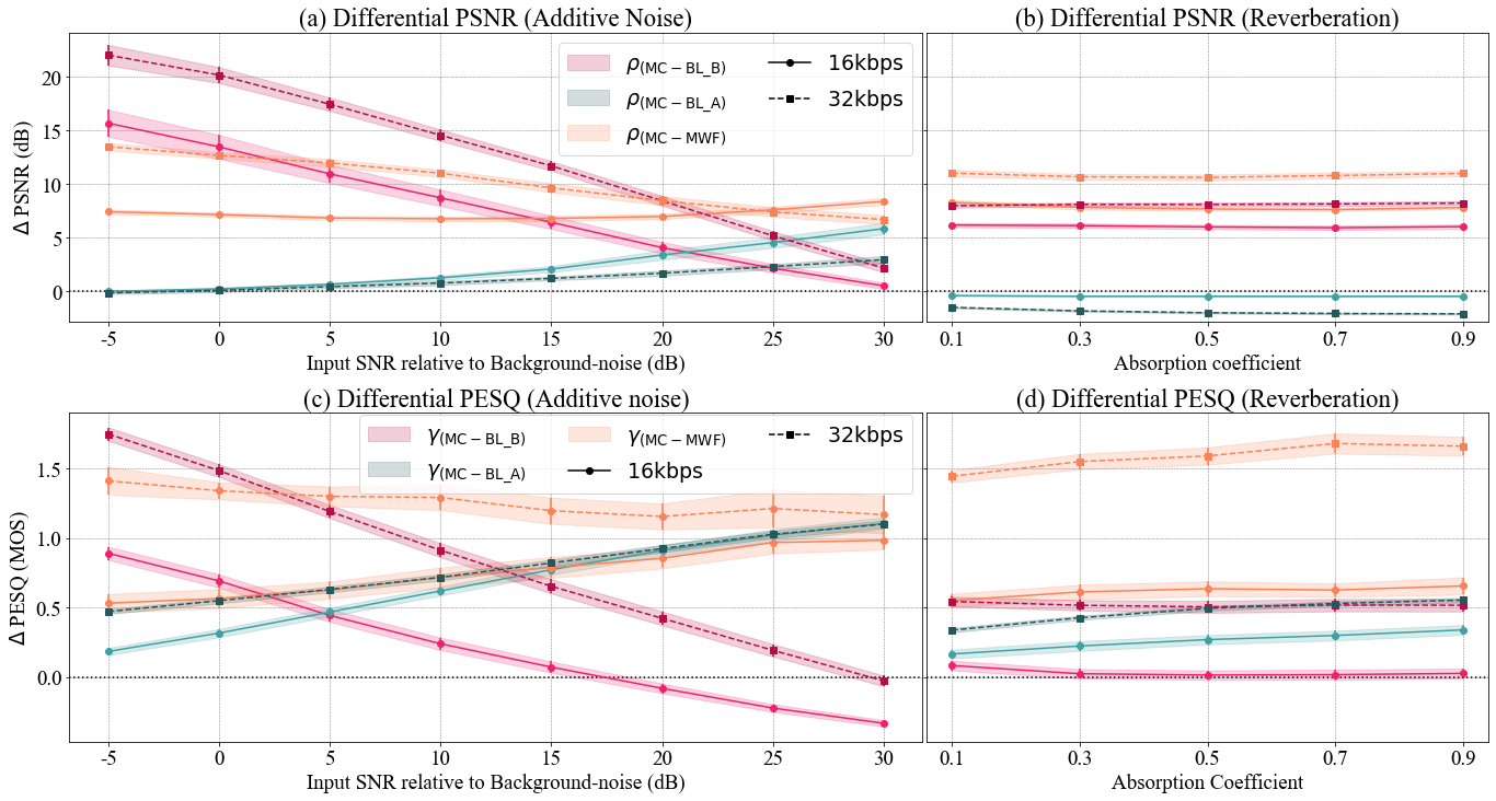
Figure 3: Illustration of differential PSNR and PESQ scores between the proposed multidevice estimate, and single-channel baseline and multichannel Wiener filter at $R=\{16,$32\text{\,}\mathrm{k}\mathrm{b}\mathrm{p}\mathrm{s}$\}$ with 95% confidence intervals. $\rho_{(\text{MC}-\text{BL\_B})}$ and $\gamma_{(\text{MC}-\text{BL\_B})}$ are the differential PSNR and PESQ of the proposed multidevice estimate with respect to single-channel estimate of device B; $\rho_{(\text{MC}-\text{BL\_A})}$ and $\gamma_{(\text{MC}-\text{BL\_A})}$ are the differential scores of the multidevice estimate with respect to single-channel estimate of device A; $\rho_{(\text{MC}-\text{MWF})}$ and $\gamma_{(\text{MC}-\text{MWF})}$ are the differential scores of the multidevice estimate with respect to the multichannel Wiener filter.

The system block diagram is depicted in Fig. 2 (a, b), where (a) is the overview of the entire system, from acoustic signal acquisition at the sensors to obtaining the time-domain estimate from multidevice signals. Note that the postfilter is placed at the fusion center, directly after the decoder, which provides the decoded perceptual domain signals to the postfilter. Fig. 2 (b) shows the internal structure of the postfilter. After receiving the quantization bin limits from the decoded signals, we compute the truncated Gaussian distribution for each channel, and then compute the joint posterior distribution as the product of the truncated distributions of the channels. The final point estimate, obtained as the expectation of the posterior distribution, yields the multidevice signal estimate.

3 Experiments and Results

To evaluate the performance of the proposed postfiltering approach, we determined the perceptual SNR (PSNR) and PESQ scores [16], and conducted a subjective listening test using MUSHRA [23, 24]. We considered two categories of degradation: 1. additive background noise, 2. background noise with reverberation. For the background noises, from the QUT dataset, we extracted the cafeteria scenario with babble noise [25]. The clean speech samples were obtained from the test set of the TIMIT dataset [26]. We encoded the noisy samples and applied the proposed postfilter to the decoded samples. Hence, the output signal is corrupted by both coding and environmental artefacts. To generate noisy speech with reverberation, we considered a room of dimensions $(7.5\times 5\times 2)$\mathrm{m}^{3}$$, with one speech source at coordinates $(1,2.5,0.5)$\mathrm{m}$$ and three noise sources placed at $(6.5,2.85,0.5)$\mathrm{m}$,(3.5,4.5,0.5)$\mathrm{m}$$ and $(6,0,0.5)$\mathrm{m}$$. The locations of the near and distant microphones are, respectively, $(1.05,2.55,0.5)$\mathrm{m}$$ and $(2.25,2.85,0.5)$\mathrm{m}$$. An illustration of the setup is presented in Fig. 1. The signals at the microphones for the described acoustic scenario were simulated using Pyroomacoustics [27].

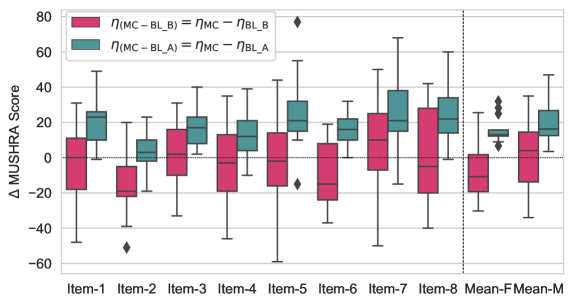
Figure 4: Distribution of $\Delta$MUSHRA points from the subjective listening test. $\eta_{(\text{MC}-\text{BL\_B})}$ and $\eta_{(\text{MC}-\text{BL\_A})}$ are the differential MUSHRA of multidevice estimate with respect to signal-channel estimates at device B and device A, respectively. Mean-F and Mean-M are the average differential scores over the female and males items, respectively.

Let $\rho$ and $\gamma$ represent the PSNR and PESQ scores, respectively and the total bitrate is $R$. The postfilter is applied on the output of a codec that is specifically suitable for multi-device coding [15]. For a fair evaluation, the single channel enhancement from Eq. 5 are used as baselines. Furthermore, we employ the conventional multichannel Wiener Filter (MWF) with diagonalized covariance matrix, to evaluate the advantage of the proposed method with respect to a conventionally accepted baseline [28]. The notations and their definitions are as follows: 1. $\hat{x}_{\text{MC}}$is the multidevice estimate using device A at the $\text{bitrate}=\frac{1}{4}R$ and device B at the $\text{bitrate}=\frac{3}{4}R$; the PSNR and PESQ scores of the estimate are $\rho_{\text{MC}}$, $\gamma_{\text{MC}}$ respectively, 2. $\hat{x}_{\text{BL\_B}}$is the baseline posterior estimate (from Eq. 5) at distant device B, encoding at full $\text{bitrate}=R$; $\rho_{\text{BL\_B}}$ and $\gamma_{\text{BL\_B}}$ are the objective measures, 3. $\hat{x}_{\text{BL\_A}}$is the baseline posterior estimate (from Eq. 5) at device A using $\text{bitrate}=\frac{1}{4}R$, and $\rho_{\text{BL\_A}}$, $\gamma_{\text{BL\_A}}$ are the objective measures, 4. $\hat{x}_{\text{MWF}}$is the multichannel Wiener filter using noisy signals from device A and device B, and $\rho_{\text{MWF}}$, $\gamma_{\text{MWF}}$ are the objective measures. We show the advantage of the proposed postfilter over the baseline methods using differential PSNR and PESQ scores; their definitions are: 1. $\rho_{(\text{MC}-\text{BL\_B})}=\rho_{\text{MC}}-\rho_{\text{BL\_B}}$, 2. $\rho_{(\text{MC}-\text{BL\_A})}=\rho_{\text{MC}}-\rho_{\text{BL\_A}}$, 3. $\rho_{(\text{MC}-\text{MWF})}=\rho_{\text{MC}}-\rho_{\text{MWF}}$, 4. $\gamma_{(\text{MC}-\text{BL\_B})}=\gamma_{\text{MC}}-\gamma_{\text{BL\_B}}$, 5. $\gamma_{(\text{MC}-\text{BL\_A})}=\gamma_{\text{MC}}-\gamma_{\text{BL\_A}}$, 6. $\gamma_{(\text{MC}-\text{MWF})}=\gamma_{\text{MC}}-\gamma_{\text{MWF}}$.

The input SNR at device A was fixed to $40\text{\,}\mathrm{d}\mathrm{B}$ and at device B, and we used a range of input $\text{SNRs}\in\{-5,0,5...,$30\text{\,}\mathrm{d}\mathrm{B}$\}$. From the test set of the TIMIT dataset, we randomly selected 100 speech samples (50 male and 50 female) and tested the postfilter over all the combinations of the bitrates, $R\in\{16,24,32,48,64,80,96$\mathrm{k}\mathrm{b}\mathrm{p}\mathrm{s}$\}$, and the input SNRs for each speech sample. The objective results for the additive noise scenario are presented in Fig. 3 (a, c). $\rho_{(\text{MC}-\text{BL\_A})}$, $\rho_{(\text{MC}-\text{BL\_B})}$ and $\rho_{(\text{MC}-\text{MWF})}$ are shown in Fig. 3 (a) for the listed SNRs and the total $\text{bitrate}\in\{16,32$\mathrm{k}\mathrm{b}\mathrm{p}\mathrm{s}$\}$; We found that the PSNR of the proposed method was better than all three baselines over all SNRs and bitrates. For $\hat{x}_{\text{MC}}$ relative to the single-channel estimate $\hat{x}_{\text{BL\_B}}$, the highest differential PSNR is $\rho_{(\text{MC}-\text{BL\_B})}\approx$22.5\text{\,}\mathrm{d}\mathrm{B}$$. With respect to $\hat{x}_{\text{BL\_A}}$, the highest $\rho_{(\text{MC}-\text{BL\_A})}\approx$6\text{\,}\mathrm{d}\mathrm{B}$$ is obtained at $30\text{\,}\mathrm{d}\mathrm{B}$ input SNR and $16\text{\,}\mathrm{k}\mathrm{b}\mathrm{p}\mathrm{s}$. In addition, we observe that $\rho_{(\text{MC}-\text{BL\_B})}$ decreases with the increase in the input SNR at device B; also, it increases with an increase in total bitrate due to lower degradation from coding noise, specifically at device A. In contrast, $\rho_{(\text{MC}-\text{BL\_A})}$ increases with an increase in the input SNR at device B but decreases with increase in the total bitrate. In terms of PESQ, the largest differential PESQ for $\hat{x}_{\text{MC}}$ relative to $\hat{x}_{\text{BL\_B}}$ is $\gamma_{(\text{MC}-\text{BL\_B})}\approx$1.8\text{\,}\mathrm{M}\mathrm{O}\mathrm{S}$$, attained at $-5\text{\,}\mathrm{d}\mathrm{B}$ and $32\text{\,}\mathrm{k}\mathrm{b}\mathrm{p}\mathrm{s}$. However, at $16\text{\,}\mathrm{k}\mathrm{b}\mathrm{p}\mathrm{s}$ and above $15\text{\,}\mathrm{d}\mathrm{B}$ the negative $\mathrm{M}\mathrm{O}\mathrm{S}$ implied a decrease in quality. With respect to $\hat{x}_{\text{BL\_A}}$, largest value is $\gamma_{(\text{MC}-\text{BL\_B})}\approx$1.1\text{\,}\mathrm{M}\mathrm{O}\mathrm{S}$$ at $30\text{\,}\mathrm{d}\mathrm{B}$ input SNR at device B. Furthermore, the variations of $\gamma_{(\text{MC}-\text{BL\_A})}$ and $\gamma_{(\text{MC}-\text{BL\_A})}$ relative to the input SNR and bitrate follow similar trends as differential PSNR. Without exception, we observed similar trends for all the listed bitrates. The inverse variations of the differential scores with respect to $\hat{x}_{\text{BL\_A}}$ and $\hat{x}_{\text{BL\_B}}$ supports our expectation that the proposed postfilter optimally merges information from the two channels to obtain an enhanced multidevice estimate.

The test was repeated to include reverberation over a range of absorption coefficients, $\alpha=\{0.1,0.3,...0.9\}$. The results for $R\in\{16,32$\mathrm{k}\mathrm{b}\mathrm{p}\mathrm{s}$\}$ are illustrated in Fig. 3 (b, d). While $\rho_{(\text{MC}-\text{BL\_B})}$ is positive for both bitrates over all the listed absorption coefficients, $\rho_{(\text{MC}-\text{BL\_A})}$ is consistently negative. One reason for this could be that while the postfilter reduces environment noise, as is reflected in the improvement with respect to $\hat{x}_{\text{BL\_B}}$, it may introduce some speech distortion, or is unable to completely remove reverberation due to the lack of reverberation model, which shows as a drop in the PSNR with respect to $\hat{x}_{\text{BL\_A}}$. Nevertheless, both $\gamma_{(\text{MC}-\text{BL\_A})}$ and $\gamma_{(\text{MC}-\text{BL\_B})}$ are positive over both the bitrates and all $\alpha$, and follow similar variation trends as in the additive noise scenario. Lastly, the positive differential objective scores for both noise types with respect to the MWF indicate that the PSNR and PESQ gains of the proposed postfilter are larger than the gains obtained using the multichannel Wiener filter. This supports our informal observation that Wiener filtering is inefficient in capturing the essential features of speech signals.

The subjective MUSHRA listening test contained eight test items (4 male and 4 female), four of which included background noise with reverberation at $\alpha=0.3$ while the remaining items comprised of background noise only at $\text{SNR}=$15\text{\,}\mathrm{d}\mathrm{B}$$. Each test item consisted of five test conditions and the reference clean speech signal; a hidden reference and a lower anchor, which was the $3.5\text{\,}\mathrm{k}\mathrm{H}\mathrm{z}$ low-pass version of the reference signal, $\hat{x}_{\text{MC}}$, $\hat{x}_{\text{BL\_B}}$, and $\hat{x}_{\text{BL\_A}}$ were presented as the test conditions; total bitrate was $R=$32\text{\,}\mathrm{k}\mathrm{b}\mathrm{p}\mathrm{s}$$. As post-screening, we retained the responses from only those subjects that rated the hidden reference at more than $90\text{\,}\mathrm{M}\mathrm{U}\mathrm{S}\mathrm{H}\mathrm{R}\mathrm{A}$ points for all items. Fig. 4 presents the consolidated differential MUSHRA, represented as $\eta$, from 13 participants who passed the post-screening; the boxplots show the median and interquartile range of $\eta$. The background noise with reverberation are presented in $\text{items}\,\{1,2,3,4\}$ and the background-noise-only samples are $\text{items}\,\{5,6,7,8\}$. $\text{Items}\,\{1,2,5,6\}$ are female and the rest are male. $\eta_{(\text{MC}-\text{BL\_A})}$ was positive for all items, indicating that most subjects preferred $\hat{x}_{\text{MC}}$ over $\hat{x}_{\text{BL\_A}}$. With respect to $\hat{x}_{\text{BL\_B}}$, the variations were found to be gender dependent. While the median $\eta_{(\text{MC}-\text{BL\_B})}$ points were positive for most male items (mean-M), they were negative for females (mean-F). Further analysis of the samples revealed that while background noise was attenuated in the $\hat{x}_{\text{MC}}$, speech distortions were introduced into the estimate and those distortions were more prominent in the female samples. This problem could potentially be addressed by using more informative speech priors, and modifying the signal model to incorporate the effects of reverberation.

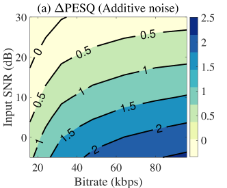
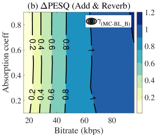
Figure 5: Contour plot showing the differential PESQ, $\gamma_{(\text{MC}-\text{BL\_B})}$ jointly over bitrates, input SNR and absorption coefficients.

To study the region of optimal performance of the postfilter, we analyzed the average $\gamma_{(\text{MC}-\text{BL\_B})}$ as a function of bitrate and input SNRs and absorption coefficient $\alpha$; the resulting contour plots are depicted in Fig. 5. For the additive background noise scenario, the highest gains are at higher bitrates and low input SNRs. Furthermore, the negative $\gamma_{(\text{MC}-\text{BL\_B})}$ over $20\text{\,}\mathrm{d}\mathrm{B}$ input SNR and below $32\text{\,}\mathrm{k}\mathrm{b}\mathrm{p}\mathrm{s}$ implies that the postfilter performs sub-optimally in this region; in other words, we gain from a multidevice signal estimate when the additive degradation level is below $20\text{\,}\mathrm{d}\mathrm{B}$ and the total bitrate is greater than $32\text{\,}\mathrm{k}\mathrm{b}\mathrm{p}\mathrm{s}$. In the presence of reverberation, we observed that while the total bitrate had an impact on $\gamma_{(\text{MC}-\text{BL\_B})}$, the improvement was fairly constant over the range of $\alpha$ at an arbitrary bitrate, and the improvement was positive over the considered input SNR range. This implies that the proposed postfilter can also be used to enhance signals degraded by reverberation and is not especially sensitive to the amount of reverberation, despite the fact that the signal model did not explicitly account for distortions from reverberation.

4 Conclusion

In this work, we proposed a postfilter to enhance speech in an ad-hoc sensor network. The method explored the feasibility of using sources degraded by two distinct noise types to obtain an enhanced estimate of the clean speech signal. We demonstrated that by distributing the total available bandwidth between two sensors, we can achieve signal quality that is higher than a single channel estimate operating at full bitrate. Further work is needed to address the classic noise-reduction vs. speech distortion problem, by incorporating a signal model which takes into account the effects of reverberation, although the objective and subjective results are already encouraging.

References

- [1] Alexander Bertrand. Applications and trends in wireless acoustic sensor networks: A signal processing perspective. In 2011 18th IEEE symposium on communications and vehicular technology in the Benelux (SCVT), pages 1–6. IEEE, 2011.
- [2] S Sandeep Pradhan and Kannan Ramchandran. Distributed source coding using syndromes (discus): Design and construction. IEEE transactions on information theory, 49(3):626–643, 2003.
- [3] Pier Luigi Dragotti and Michael Gastpar. Distributed source coding: theory, algorithms and applications. Academic Press, 2009.
- [4] T Bäckström. Speech Coding with Code-Excited Linear Prediction. Springer, 2017.
- [5] Tom Bäckström and Johannes Fischer. Fast randomization for distributed low-bitrate coding of speech and audio. IEEE/ACM Transactions on Audio, Speech, and Language Processing, 26(1):19–30, 2017.
- [6] T. Bäckström and J. Fischer. Coding of parametric models with randomized quantization in a distributed speech and audio codec. In Proceedings of the 12. ITG Symposium on Speech Communication, pages 1–5. VDE, 2016.
- [7] Adel Zahedi, Jan Østergaard, Søren Holdt Jensen, Patrick Naylor, and Søren Bech. Coding and enhancement in wireless acoustic sensor networks. In 2015 Data Compression Conference, pages 293–302. IEEE, 2015.
- [8] Olivier Roy and Martin Vetterli. Rate-constrained collaborative noise reduction for wireless hearing aids. IEEE Transactions on Signal Processing, 57(2):645–657, 2008.
- [9] Sriram Srinivasan and Albertus C Den Brinker. Rate-constrained beamforming in binaural hearing aids. EURASIP Journal on Advances in Signal Processing, 2009(1):257197, 2009.
- [10] Sriram Srinivasan and Albertus C Den Brinker. Analyzing rate-constrained beamforming schemes in wireless binaural hearing aids. In 2009 17th European Signal Processing Conference, pages 1854–1858. IEEE, 2009.
- [11] Simon Doclo, Marc Moonen, Tim Van den Bogaert, and Jan Wouters. Reduced-bandwidth and distributed mwf-based noise reduction algorithms for binaural hearing aids. IEEE Transactions on Audio, Speech, and Language Processing, 17(1):38–51, 2009.
- [12] J. Amini, R. C. Hendriks, R. Heusdens, M. Guo, and J. Jensen. Asymmetric coding for rate-constrained noise reduction in binaural hearing aids. IEEE/ACM Transactions on Audio, Speech, and Language Processing, 27(1):154–167, 2019.
- [13] Jamal Amini, Richard Christian Hendriks, Richard Heusdens, Meng Guo, and Jesper Jensen. Rate-constrained noise reduction in wireless acoustic sensor networks. IEEE/ACM Transactions on Audio, Speech, and Language Processing, 28:1–12, 2019.
- [14] Jie Zhang, Sundeep Prabhakar Chepuri, Richard Christian Hendriks, and Richard Heusdens. Microphone subset selection for mvdr beamformer based noise reduction. IEEE/ACM Transactions on Audio, Speech, and Language Processing, 26(3):550–563, 2017.
- [15] Tom Bäckström, Johannes Fischer, Sneha Das, et al. Dithered quantization for frequency-domain speech and audio coding. In Interspeech, pages 3533–3537, 2018.
- [16] T. Bäckström. Speech Coding with Code-Excited Linear Prediction. Springer, 2017.
- [17] Kiseon Kim and Georgy Shevlyakov. Why gaussianity? IEEE Signal Processing Magazine, 25(2):102–113, 2008.
- [18] Simo Särkkä. Bayesian filtering and smoothing, volume 3. Cambridge University Press, 2013.
- [19] S. Das and T. Bäckström. Postfiltering with complex spectral correlations for speech and audio coding. In Interspeech, 2018.
- [20] Donald R Barr and E Todd Sherrill. Mean and variance of truncated normal distributions. The American Statistician, 53(4):357–361, 1999.
- [21] Rainer Martin. Noise power spectral density estimation based on optimal smoothing and minimum statistics. IEEE Transactions on speech and audio processing, 9(5):504–512, 2001.
- [22] Robert M McLeod. The generalized Riemann integral, volume 20. American Mathematical Soc., 1980.
- [23] ITU-R. Method for the subjective assessment of intermediate quality level of audio systems. International Telecommunication Union Radiocommunication Assembly, 2014.
- [24] M. Schoeffler, F. R. Stöter, B. Edler, and J. Herre. Towards the next generation of web-based experiments: a case study assessing basic audio quality following the ITU-R recommendation BS. 1534 (MUSHRA). In 1st Web Audio Conference. Citeseer, 2015.
- [25] David B Dean, Sridha Sridharan, Robert J Vogt, and Michael W Mason. The qut-noise-timit corpus for the evaluation of voice activity detection algorithms. Proceedings of Interspeech 2010, 2010.
- [26] V Zue, S Seneff, and J Glass. Speech database development at MIT: TIMIT and beyond. Speech Communication, 9(4):351–356, 1990.
- [27] Robin Scheibler, Eric Bezzam, and Ivan Dokmanić. Pyroomacoustics: A python package for audio room simulation and array processing algorithms. In 2018 IEEE International Conference on Acoustics, Speech and Signal Processing (ICASSP), pages 351–355. IEEE, 2018.
- [28] S. Doclo and M. Moonen. Gsvd-based optimal filtering for single and multimicrophone speech enhancement. IEEE Transactions on Signal Processing, 50(9):2230–2244, 2002.