Symmetric Parallax Attention for Stereo Image Super-Resolution

Abstract

Although recent years have witnessed the great advances in stereo image super-resolution (SR), the beneficial information provided by binocular systems has not been fully used. Since stereo images are highly symmetric under epipolar constraint, in this paper, we improve the performance of stereo image SR by exploiting symmetry cues in stereo image pairs. Specifically, we propose a symmetric bi-directional parallax attention module (biPAM) and an inline occlusion handling scheme to effectively interact cross-view information. Then, we design a Siamese network equipped with a biPAM to super-resolve both sides of views in a highly symmetric manner. Finally, we design several illuminance-robust losses to enhance stereo consistency. Experiments on four public datasets demonstrate the superior performance of our method. Source code is available at https://github.com/YingqianWang/iPASSR.

1 Introduction

With recent advances in stereo vision, dual cameras are commonly adopted in mobile phones and autonomous vehicles. Using the complementary information (i.e., cross-view information) provided by binocular systems, the resolution of image pairs can be enhanced. However, it is challenging to achieve good performance in stereo image super-resolution (SR) due to the following issues: 1) Varying parallax. Objects at different depths have different disparity values and thus locate at different positions along the horizontal epipolar line. It is challenging to capture reliable stereo correspondence and effectively integrate cross-view information for stereo image SR. 2) Information incorporation. Since context information within a single view (i.e., intra-view information) is crucial and contributes to stereo image SR in a different manner, it is important but challenging to fully incorporate both intra-view and cross-view information. 3) Occlusions & boundaries. In occlusion and boundary areas, pixels in one view cannot find their correspondence in the other view. In this case, only intra-view information is available for stereo image SR. It is challenging to fully use cross-view information in non-occluded regions while maintaining promising performance in occluded regions.

Recently, several methods have been proposed to address the above issues. Wang et al.[23, 25] addressed the varying parallax issue by proposing a parallax attention module (PAM), and developed a PASSRnet for stereo image SR. Ying et al.[32] addressed the information incorporation issue by equipping several stereo attention modules (SAMs) to the pre-trained single image SR (SISR) networks. Song et al.[19] addressed the occlusion issue by checking stereo consistency using disparity maps regressed by parallax attention maps. Although continuous improvements have been achieved, the inherent correlation within stereo image pairs are still under exploited, which hinders the performance of stereo image SR.

Since super-resolving left and right images are highly symmetric, the inherent correlation within an image pair can be fully used by exploiting its symmetry cues. In this paper, we improve the performance of stereo image SR by exploiting symmetries on three levels. 1) On the module level, we design a symmetric bi-directional parallax attention module (biPAM) to interact cross-view information. With our biPAM, occlusion maps can be generated and used as a guidance for cross-view feature fusion. 2) On the network level, we propose a Siamese network equipped with our biPAM to super-resolve both left and right images. Experimental results demonstrate that jointly super-resolving both sides of views can better exploit the correlation between stereo images and is contributive to SR performance. 3) On the optimization level, we exploit symmetry cues by designing several bilateral losses. Our proposed losses can enforce stereo consistency and is robust to illuminance changes between stereo images. We perform extensive ablation studies to validate the effectiveness of our method. Comparative results on the KITTI 2012 [4], KITTI 2015 [14], Middlebury [17] and Flickr1024 [27] datasets have demonstrated the competitive performance of our method as compared to many state-of-the-art SR methods.

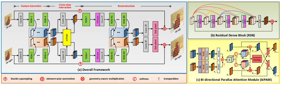
Figure 1: An overview of our iPASSR network.

Our proposed method is named iPASSR since it is an improved version of our previous PASSRnet [23, 25]. The contributions of this paper are as follows: 1) We propose to exploit symmetry cues for stereo image SR. Different from PASSRnet, our iPASSR can super-resolve both sides of views within a single inference. 2) We develop a symmetric and bi-directional parallax attention module. Compared to PAMs in [23, 25], our biPAM is more compact and can effectively handle occlusions. 3) As demonstrated in the experiments, our iPASSR can achieve significant performance improvements over PASSRnet with a comparable model size.

The rest of this paper is organized as follows. In Section 2, we briefly review the related work. In Section 3, we introduce our proposed method including network architecture, occlusion handling scheme, and loss functions. Experimental results are presented in Section 4. Finally, we conclude this paper in Section 5.

2 Related Work

Single Image SR. SISR is a long-standing problem and has been investigated for decades. Recently, deep learning-based SISR methods have achieved promising performance in terms of both reconstruction accuracy [33, 35, 22, 24] and visual quality [11, 26, 1, 34]. Dong et al.[3] proposed the first CNN-based SR network named SRCNN to reconstruct high-resolution (HR) images from low-resolution (LR) inputs. Kim et al.[8] proposed a very deep network (VDSR) with 20 layers to improve SR performance. Afterwards, SR networks became increasingly deep and complex, and thus more powerful in intra-view information exploitation. Lim et al.[12] proposed an enhanced deep SR network (EDSR) using both local and global residual connections. Zhang et al.[38, 39] combined residual connection with dense connection, and proposed residual dense network (RDN) to fully exploit hierarchical feature representations. More recently, the performance of SISR has been further improved by RCAN [36], RNAN [37] and SAN [2].

Stereo Image SR. Compared to SISR which exploits context information within only one view, stereo image SR aims at using the cross-view information provided by stereo images. Jeon et al.[6] proposed a network named StereoSR to learn a parallax prior by jointly training two cascaded sub-networks. The cross-view information is integrated by concatenating the left image and a stack of right images with different pre-defined shifts. Wang et al.[23, 25] proposed a parallax attention module to learn stereo correspondence with a global receptive field along the epipolar line. Ying et al.[32] proposed a stereo attention module and embedded it into pre-trained SISR networks for stereo image SR. Song et al.[19] combined self-attention with parallax attention for stereo image SR. Furthermore, stereo consistency was addressed by using disparity maps regressed from parallax attention maps. Yan et al.[29] proposed a domain adaptive stereo SR network (, DASSR). Specifically, they first explicitly estimated disparities using a pretrained stereo matching network [7] and then warped views to the other side to incorporate cross-view information. More recently, Xu et al.[28] incorporated bilateral grid processing into CNNs and proposed a BSSRnet for stereo image SR.

3 Method

In this section, we introduce our method in details. We first introduce the architecture of our network in Section 3.1, then describe the inline occlusion handling scheme in Section 3.2. Finally, we present the losses in Section 3.3.

3.1 Network Architecture

Our network takes a pair of LR RGB stereo images $\mathbf{I}_{\text{L}}^{\text{input}}$ and $\mathbf{I}_{\text{R}}^{\text{input}}$ as its inputs to generate HR RGB stereo images $\mathbf{I}_{\text{L}}^{\text{SR}}$ and $\mathbf{I}_{\text{R}}^{\text{SR}}$. As shown in Fig. 1(a), our network is highly symmetric and the weights of its left and right branches are shared. Given LR input stereo images, our network sequentially performs feature extraction, cross-view interaction, and reconstruction.

Feature Extraction. In our feature extraction module, input stereo images $\mathbf{I}_{\text{L}}^{\text{input}},\mathbf{I}_{\text{R}}^{\text{input}}\in\mathbb{R}^{H\times W\times 3}$ are first fed to a convolution layer (, Conv-0) to generate initial features $\mathbf{F}_{\text{L}}^{0},\mathbf{F}_{\text{R}}^{0}\in\mathbb{R}^{H\times W\times 64}$, which are then fed to 4 cascaded residual dense blocks (RDBs) for deep feature extraction. As shown in Fig. 1(b), 4 convolutions with a growth rate of 24 are used within each RDB to achieve dense feature representation. Note that, features from all the layers in an RDB are concatenated and fed to a 1$\times$1 convolution to generate fused features for local residual connection.

Cross-view Interaction. We propose a bi-directional parallax attention module (biPAM) to interact cross-view information of stereo features. Since hierarchical feature representation is beneficial to stereo correspondence learning [23], we form the inputs of our biPAM by concatenating the output features of each RDB in our feature extraction module. As shown in Fig. 1(c), the input stereo features are first fed to a batch-normalization (BN) layer and a transition residual block (, ResB), and then separately fed to 1$\times$1 convolutions to generate $\mathbf{F}_{\text{U}}$, $\mathbf{F}_{\text{V}}\in\mathbb{R}^{H\times W\times 64}$. To achieve disentangled pairwise parallax attention, we follow [31] and feed $\mathbf{F}_{\text{U}}$ and $\mathbf{F}_{\text{V}}$ to a whiten layer to obtain normalized features $\mathbf{F}^{\prime}_{\text{U}}$ and $\mathbf{F}^{\prime}_{\text{V}}$ according to

$$\mathbf{F}^{\prime}_{\text{U}}(h,w,c)=\mathbf{F}_{\text{U}}(h,w,c)-\frac{1}{W}\sum\nolimits_{i=1}^{W}\mathbf{F}_{\text{U}}(h,i,c),$$ (1)

$$\mathbf{F}^{\prime}_{\text{V}}(h,w,c)=\mathbf{F}_{\text{V}}(h,w,c)-\frac{1}{W}\sum\nolimits_{i=1}^{W}\mathbf{F}_{\text{V}}(h,i,c).$$ (2)

To generate left and right attention maps, $\mathbf{F}^{\prime}_{\text{V}}$ is first transposed to ${\mathbf{F}^{\prime}_{\text{V}}}^{\text{T}}\in\mathbb{R}^{H\times 64\times W}$, and then batch-wisely multiplied (see Section 3.2) with $\mathbf{F}^{\prime}_{\text{U}}$ to produce an initial score map $\mathbf{S}\in\mathbb{R}^{H\times W\times W}$. Then, softmax normalization is applied to $\mathbf{S}$ and $\mathbf{S}^{\text{T}}$ along their last dimension to generate attention maps $\mathbf{M}_{\text{R$\rightarrow$L}}$ and $\mathbf{M}_{\text{L$\rightarrow$R}}$, respectively. To achieve cross-view interaction, both left and right features (generated by Conv-1f in Fig. 1(a)) need to be converted to the other side by taking a batch-wise matrix multiplication with the corresponding attention maps, ,

$$\mathbf{F^{\prime}}_{\text{R$\rightarrow$L}}=\mathbf{M}_{\text{R$\rightarrow$L}}\otimes\mathbf{F}_{\text{R}},$$ (3)

$$\mathbf{F^{\prime}}_{\text{L$\rightarrow$R}}=\mathbf{M}_{\text{L$\rightarrow$R}}\otimes\mathbf{F}_{\text{L}},$$ (4)

where $\otimes$ denotes the batch-wise matrix multiplication.

To avoid unreliable correspondence in occlusion and boundary regions, we propose an inline occlusion handling scheme to calculate valid masks $\mathbf{V}_{\text{L}}$ and $\mathbf{V}_{\text{R}}$. The final converted features $\mathbf{F}_{\text{R$\rightarrow$L}}$ and $\mathbf{F}_{\text{L$\rightarrow$R}}$ can be obtained by

$$\mathbf{F}_{\text{R$\rightarrow$L}}=\mathbf{V}_{\text{L}}\odot\mathbf{F^{\prime}}_{\text{R$\rightarrow$L}}+(\mathbf{1}-\mathbf{V}_{\text{L}})\odot\mathbf{F}_{\text{L}},$$ (5)

$$\mathbf{F}_{\text{L$\rightarrow$R}}=\mathbf{V}_{\text{R}}\odot\mathbf{F^{\prime}}_{\text{L$\rightarrow$R}}+(\mathbf{1}-\mathbf{V}_{\text{R}})\odot\mathbf{F}_{\text{R}},$$ (6)

where $\odot$ represents element-wise multiplication. Note that, values in $\mathbf{V}_{\text{L}}$ and $\mathbf{V}_{\text{R}}$ range from 0 (occluded) to 1 (non-occluded). According to Eqs. (5) and (6), occluded regions of converted features (, $\mathbf{F}_{\text{R$\rightarrow$L}}$, $\mathbf{F}_{\text{L$\rightarrow$R}}$) can be filled with the corresponding features from the target view (, $\mathbf{F}_{\text{L}}$, $\mathbf{F}_{\text{R}}$), resulting in continuous spatial distributions.

Reconstruction. Similar to the feature extraction module, we use RDB as the basic block in our reconstruction module. Taking the left branch as an example, $\mathbf{F}_{\text{R}\rightarrow\text{L}}$ is first concatenated with $\mathbf{F}_{\text{L}}$ and then fed to an RDB (, RDB-F) for initial feature fusion. The output feature $\mathbf{F}_{\text{L}}^{\text{init\_f}}\in\mathbb{R}^{H\times W\times 128}$ is then fed to a channel attention layer (, CALayer [36]) and a convolution layer (, Conv-2f) to produce the final fused feature $\mathbf{F}_{\text{L}}^{\text{f}}\in\mathbb{R}^{H\times W\times 64}$. Afterwards, $\mathbf{F}_{\text{L}}^{\text{f}}$ is fed to 4 cascaded RDBs, a convolution layer (, Conv-3f), and a sub-pixel layer [18] to generate the super-resolved left image $\mathbf{I}_{\text{L}}^{\text{SR}}$.

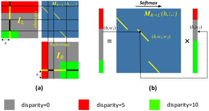
Figure 2: A toy example to depict the stereo correspondence. The gray, red, and green regions in $\mathbf{I}_{\text{L}}$ and $\mathbf{I}_{\text{R}}$ denote objects with a disparity of $0$, $5$, and $10$ pixels, respectively. For simplicity, only a profile of $\mathbf{M}_{\text{R$\rightarrow$L}}$ at height $h$ is visualized, which corresponds to the regions marked by yellow strokes in (a). Occlusions (colored in black on the strokes) are implicitly encoded in the attention maps as empty intervals. (b) The right stroke can be converted into the left side by multiplying it with $\mathbf{M}_{\text{R$\rightarrow$L}}$.

3.2 Inline Occlusion Handling Scheme

By using biPAM, the stereo correspondence can be generated in a symmetric manner. More importantly, the occlusions can be derived by checking the stereo consistency using the attention maps $\mathbf{M}_{\text{R$\rightarrow$L}}$ and $\mathbf{M}_{\text{L$\rightarrow$R}}$.

Here, we use a toy example in Fig. 2 to illustrate how occlusions are implicitly encoded in the parallax attention maps. Given a pair of stereo images $\mathbf{I}_{\text{L}}$ and $\mathbf{I}_{\text{R}}\in\mathbb{R}^{H\times W}$, parallax attention maps $\mathbf{M}_{\text{R$\rightarrow$L}},\mathbf{M}_{\text{L$\rightarrow$R}}\in\mathbb{R}^{H\times W\times W}$ can be generated. As illustrated in Fig. 2(a), we visualize a profile of $\mathbf{M}_{\text{R$\rightarrow$L}}$ at height $h$ (, $\mathbf{M}_{\text{R$\rightarrow$L}}(h,:,:)$), which corresponds to the yellow strokes in the left and right images. Note that, black strokes represent occluded regions. It can be observed from Fig. 2(a) that: 1) Occlusions occur near object edges where the depth values change suddenly, or occur near image boundaries (more specifically, left boundary of the left view and right boundary of the right view). 2) The occluded regions correspond to the empty intervals in the attention maps since their counterparts in the other view are unavailable. These two observations demonstrate that occlusions are implicitly encoded in the parallax attention maps and can be calculated by checking the cycle consistency using $\mathbf{M}_{\text{R$\rightarrow$L}}$ and $\mathbf{M}_{\text{L$\rightarrow$R}}$. Specifically, the right image can be converted into the left side according to $\mathbf{I}_{\text{R$\rightarrow$L}}=\mathbf{M}_{\text{R$\rightarrow$L}}\otimes\mathbf{I}_{\text{R}}$, where $\otimes$ represents the batch-wise matrix multiplication. As shown in Fig. 2(b), the product of a slice of the right image (, $\mathbf{I}_{\text{R}}(h,:)$) and the corresponding profile of the attention map (, $\mathbf{M}_{\text{R$\rightarrow$L}}(h,:,:)$) determines the slice of the converted left image at the same height (, $\mathbf{I}_{\text{R$\rightarrow$L}}(h,:)$). All these resulting slices are concatenated to produce $\mathbf{I}_{\text{R$\rightarrow$L}}$.

Note that, softmax normalization has been performed along the third dimension of $\mathbf{M}_{\text{R$\rightarrow$L}}$ and $\mathbf{M}_{\text{L$\rightarrow$R}}$. Therefore, $\mathbf{M}_{\text{R$\rightarrow$L}}(h,w_{1},w_{2})$ can be considered as the matching possibility between $\mathbf{I}_{\text{R}}(h,w_{2})$ and $\mathbf{I}_{\text{L}}(h,w_{1})$. Furthermore, the possibility that $\mathbf{I}_{\text{L}}(h,w_{1})$ is first converted to $\mathbf{I}_{\text{R}}$ and then re-converted to $\mathbf{I}_{\text{L}}(h,w_{1})$ can be calculated according to

$$\mathbf{P}_{\text{L}}(h,w_{1})=\sum_{w_{2}=1}^{W}\mathbf{M}_{\text{R$\rightarrow$L}}(h,w_{1},w_{2})\cdot\mathbf{M}_{\text{L$\rightarrow$R}}(h,w_{2},w_{1}).$$ (7)

Note that, $\mathbf{P}_{\text{L}}(h,w_{1})$ is close to 0 if point $(h,w_{1})$ is occluded in the right view. Consequently, $\mathbf{P}_{\text{L}}$ can be used to represent occlusions in the left image. Due to noise and rectification errors in stereo images, we relax the constraint in Eq. 7 by $\pm 2$ pixels in this work:

$$\begin{split}\mathbf{P}^{\prime}_{\text{L}}(h,w_{1})=\sum_{\delta=-2}^{2}\sum_{w_{2}=1}^{W}&\mathbf{M}_{\text{R$\rightarrow$L}}(h,w_{1}+\delta,w_{2})\cdot\\ &\mathbf{M}_{\text{L$\rightarrow$R}}(h,w_{2},w_{1}).\end{split}$$ (8)

To maintain training stability, the left valid mask $\mathbf{V}_{\text{L}}$ is calculated according to $\mathbf{V}_{\text{L}}=\text{tanh}(\tau\mathbf{P}^{\prime}_{\text{L}})$, where $\tau$ was empirically set to 5 in our implementation. The right valid mask $\mathbf{V}_{\text{R}}$ can be generated following a similar way. Figure 3 shows some examples of the generated valid masks.

3.3 Losses

The overall loss function of our network is defined as:

$$\mathcal{L}=\mathcal{L}_{\text{SR}}+\lambda(\mathcal{L}_{\text{photo}}^{\text{res}}+\mathcal{L}_{\text{cycle}}^{\text{res}}+\mathcal{L}_{\text{smooth}}+\mathcal{L}_{\text{cons}}^{\text{res}}),$$ (9)

where $\mathcal{L}_{\text{SR}}$, $\mathcal{L}_{\text{photo}}^{\text{res}}$, $\mathcal{L}_{\text{cycle}}^{\text{res}}$, $\mathcal{L}_{\text{smooth}}$, and $\mathcal{L}_{\text{cons}}^{\text{res}}$ represent SR loss, residual photometric loss, residual cycle loss, smoothness loss, and residual stereo consistency loss, respectively. $\lambda$ represents the weight of the regularization term and was empirically set to 0.1 in this work. The SR loss is defined as the $L_{1}$ distance between the super-resolved and groundtruth stereo images:

$$\mathcal{L}_{\text{SR}}=\parallel\mathbf{I}_{\text{L}}^{\text{SR}}-\mathbf{I}_{\text{L}}^{\text{HR}}\parallel_{1}+\parallel\mathbf{I}_{\text{R}}^{\text{SR}}-\mathbf{I}_{\text{R}}^{\text{HR}}\parallel_{1},$$ (10)

where $\mathbf{I}_{\text{L}}^{\text{SR}}$ and $\mathbf{I}_{\text{R}}^{\text{SR}}$ represent the super-resolved left and right images, $\mathbf{I}_{\text{L}}^{\text{HR}}$ and $\mathbf{I}_{\text{R}}^{\text{HR}}$ represent their groundtruth HR images.

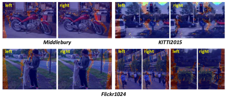
Figure 3: An illustration of valid masks generated by our occlusion handling scheme. Red regions have small values and represent heavy occlusions.

Due to exposure difference and non-Lambertain surfaces, the illuminance intensity between stereo images can vary significantly (see Fig. 4). In these cases, the photometric loss and cycle loss used in [25, 23, 32, 19] can lead to a mismatch problem. To handle this problem, we calculate these losses using residual images to improve their robustness to illuminance changes. Specifically, we introduce $\mathbf{X}_{\text{L}}=\left|\mathbf{I}_{\text{L}}^{\text{HR}}-\mathbf{I}_{\text{L}}^{\text{LR}}\uparrow\right|\downarrow$ and $\mathbf{X}_{\text{R}}=\left|\mathbf{I}_{\text{R}}^{\text{HR}}-\mathbf{I}_{\text{R}}^{\text{LR}}\uparrow\right|\downarrow$, where $\uparrow$ and $\downarrow$ represent bicubic upsampling and downsampling, and $\mathbf{X}_{\text{L}}$ and $\mathbf{X}_{\text{R}}$ represent the absolute values of the left and right residual images, respectively. Consequently, the residual photometric loss and residual cycle consistency loss can be formulated as:

$$\begin{split}\mathcal{L}_{\text{photo}}^{\text{res}}&=\parallel V_{\text{L}}\odot(\mathbf{X}_{\text{L}}-\mathbf{M}_{\text{R$\rightarrow$ L}}\otimes\mathbf{X}_{\text{R}})\parallel_{1}\\ &+\parallel V_{\text{R}}\odot(\mathbf{X}_{\text{R}}-\mathbf{M}_{\text{L$\rightarrow$R}}\otimes\mathbf{X}_{\text{L}})\parallel_{1},\end{split}$$ (11)

$$\begin{split}\mathcal{L}_{\text{cycle}}^{\text{res}}&=\parallel V_{\text{L}}\odot(\mathbf{X}_{\text{L}}-\mathbf{M}_{\text{R$\rightarrow$L}}\otimes\mathbf{M}_{\text{L$\rightarrow$R}}\otimes\mathbf{X}_{\text{L}})\parallel_{1}\\ &+\parallel V_{\text{R}}\odot(\mathbf{X}_{\text{R}}-\mathbf{M}_{\text{L$\rightarrow$R}}\otimes\mathbf{M}_{\text{R$\rightarrow$L}}\otimes\mathbf{X}_{\text{R}})\parallel_{1}.\end{split}$$ (12)

Residual photometric and cycle losses introduce two benefits. First, since illuminance components can be eliminated, more consistent and illuminance-robust stereo correspondence can be learned by our biPAM. Second, since residual images mainly contain high-frequency components, our biPAM can pay more attention to texture-rich regions, which is contributive to SR performance.

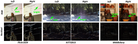
Figure 4: An illustration of illuminance changes in stereo image pairs. View our demo video for better visualization.

Apart from the aforementioned losses, we also employ smoothness loss to encourage smoothness in correspondence space. That is,

$$\begin{split}\mathcal{L}_{\text{smooth}}&=\sum_{\mathbf{M}}\sum_{i,j,k}(\parallel\mathbf{M}(i,j,k)-\mathbf{M}(i+1,j,k)\parallel_{1}\\ &+\parallel\mathbf{M}(i,j,k)-\mathbf{M}(i,j+1,k+1)\parallel_{1}),\end{split}$$ (13)

where $\mathbf{M}\in\{\mathbf{M}_{\text{R$\rightarrow$L}},\mathbf{M}_{\text{L$\rightarrow$R}}\}$. Here, $\parallel\mathbf{M}_{\text{R$\rightarrow$L}}(i,j,k)-\mathbf{M}_{\text{R$\rightarrow$L}}(i+1,j,k)\parallel_{1}$ enforces the correspondence between $\mathbf{I}_{\text{R}}(i+1,k)$ and $\mathbf{I}_{\text{L}}(i+1,j)$ to be close to the correspondence between $\mathbf{I}_{\text{R}}(i,k)$ and $\mathbf{I}_{\text{L}}(i,j)$.

Finally, we introduce residual stereo consistency loss to achieve stereo consistency between super-resolved left and right images. Specifically, the LR residuals between super-resolved images and groundtruth images are calculated according to $\mathbf{Y}_{\text{L}}=\left|\mathbf{I}_{\text{L}}^{\text{HR}}-\mathbf{I}_{\text{L}}^{\text{SR}}\right|\downarrow$ and $\mathbf{Y}_{\text{R}}=\left|\mathbf{I}_{\text{R}}^{\text{HR}}-\mathbf{I}_{\text{R}}^{\text{SR}}\right|\downarrow$, respectively, and the residual stereo consistency loss is defined as

$$\begin{split}\mathcal{L}_{\text{cons}}^{\text{res}}&=\parallel V_{\text{L}}\odot(\mathbf{Y}_{\text{L}}-\mathbf{M}_{\text{R$\rightarrow$L}}\otimes\mathbf{Y}_{\text{R}})\parallel_{1}\\ &+\parallel V_{\text{R}}\odot(\mathbf{Y}_{\text{R}}-\mathbf{M}_{\text{L$\rightarrow$R}}\otimes\mathbf{Y}_{\text{L}})\parallel_{1}.\end{split}$$ (14)

4 Experiments

In this section, we first introduce the datasets and implementation details, then perform ablation studies to validate our design choices. Finally, we compare our iPASSR to several state-of-the-art SISR and stereo image SR methods.

4.1 Datasets and Implementation Details

We used 800 images from the training set of Flickr1024 [27] and 60 images from Middlebury [17] as the training data. For images from the Middlebury dataset, we followed [6, 25, 32] to perform bicubic downsampling with a factor of 2 to generate HR images. For test, we followed [6, 25, 32] to generate our test set by using 5 images from Middlebury [17], 20 images from KITTI 2012 [4] and 20 images from KITTI 2015 [14]. Moreover, we used the test set of Flickr1024 [27] for additional evaluation. We used the bicubic downsampling approach to generate LR images. During the training phase, the generated LR images were cropped into patches of size $30\times 90$ with a stride of 20, and their HR counterparts were cropped accordingly. These patches were randomly flipped horizontally and vertically for data augmentation.

Peak signal-to-noise ratio (PSNR) and structural similarity (SSIM) were used as quantitative metrics. To achieve fair comparison with [6, 25, 32], we followed these methods to calculate PSNR and SSIM on the left views with their left boundaries (64 pixels) being cropped. Moreover, to comprehensively evaluate the performance of stereo image SR, we also report the average PSNR and SSIM scores on stereo image pairs (, $\left(\textit{Left}+\textit{Right}\right)/2$) without any boundary cropping.

Our network was implemented in PyTorch on a PC with two Nvidia RTX 2080Ti GPUs. All models were optimized using the Adam method with $\beta_{1}=0.9$, $\beta_{2}=0.999$ and a batch size of 36. The initial learning rate was set to $2\times 10^{-4}$ and reduced to half after every 30 epochs. The training was stopped after 80 epochs since more epochs do not provide further consistent improvement.

4.2 Ablation Study

Table 1: Results achieved on the KITTI 2015 dataset by our method with different cross-view information incorporation schemes for $4\times$SR. Here, PSNR$/$SSIM of the cropped left views are reported.

Models	Inputs	PSNR$/$SSIM
iPASSR with single input	Left	25.316$/$0.7753
iPASSR with replicated inputs	Left-Left	25.400$/$0.7775
Asymmetric iPASSR	Left-Right	25.548$/$0.7829
iPASSR	Left-Right	25.615$/$0.7850

Cross-view information. We removed biPAM and retrained a single branch of our iPASSR on the same training set as our original network. In addition, we also used pairs of replicated left images as inputs to directly perform inference using our original network. As shown in Table 1, the network trained with single images (, iPASSR with single input) suffers a decrease of 0.299 dB in PSNR as compared to the original network. If replicated left images were used as inputs, the performance of the variant (, iPASSR with replicated inputs) is also notably inferior to our original network. These results demonstrate the importance of cross-view information for stereo image SR.

Siamese network architecture. We investigate the benefits introduced by our Siamese network architecture by retraining the network with stereo images as inputs but only super-resolving the left view (, Asymmetric iPASSR). It can be observed in Table 1 that the PSNR score achieved by Asymmetric iPASSR is marginally lower than our iPASSR (25.548 v.s. 25.615). That is because, the symmetric Siamese network structure can help to better exploit the cross-view information to improve the SR performance.

Table 2: Results achieved on the KITTI 2015 dataset [14] by iPASSR with different losses for $4\times$SR. “Res” represents $\mathcal{L}_{\text{photo}}$, $\mathcal{L}_{\text{cycle}}$, and $\mathcal{L}_{\text{cons}}$ calculated on residual images. Here, PSNR$/$SSIM values of the cropped left views are reported.

$\mathcal{L}_{\text{SR}}$	$\mathcal{L}_{\text{photo}}$	$\mathcal{L}_{\text{smooth}}$	$\mathcal{L}_{\text{cycle}}$	$\mathcal{L}_{\text{cons}}$	Res	PSNR$/$SSIM
$\checkmark$						25.527$/$0.7827
$\checkmark$	$\checkmark$				$\checkmark$	25.535$/$0.7815
$\checkmark$	$\checkmark$	$\checkmark$			$\checkmark$	25.481$/$0.7795
$\checkmark$	$\checkmark$		$\checkmark$		$\checkmark$	25.552$/$0.7839
$\checkmark$	$\checkmark$	$\checkmark$	$\checkmark$		$\checkmark$	25.570$/$0.7839
$\checkmark$	$\checkmark$	$\checkmark$	$\checkmark$	$\checkmark$		25.456$/$0.7775
$\checkmark$	$\checkmark$	$\checkmark$	$\checkmark$	$\checkmark$	$\checkmark$	25.615$/$0.7850

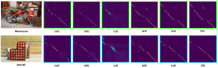
Figure 5: Visualization of attention maps generated by our iPASSR trained with different losses. (a) $\mathcal{L}_{\text{SR}}$, (b) $\mathcal{L}_{\text{SR}}+\lambda\mathcal{L}_{\text{photo}}^{\text{res}}$, (c) $\mathcal{L}_{\text{SR}}+\lambda(\mathcal{L}_{\text{photo}}^{\text{res}}+\mathcal{L}_{\text{smooth}})$, (d) $\mathcal{L}_{\text{SR}}+\lambda(\mathcal{L}_{\text{photo}}^{\text{res}}+\mathcal{L}_{\text{cycle}}^{\text{res}})$, (e) $\mathcal{L}_{\text{SR}}+\lambda(\mathcal{L}_{\text{photo}}^{\text{res}}+\mathcal{L}_{\text{smooth}}+\mathcal{L}_{\text{cycle}}^{\text{res}})$, (f) $\mathcal{L}_{\text{SR}}+\lambda(\mathcal{L}_{\text{photo}}^{\text{res}}+\mathcal{L}_{\text{smooth}}+\mathcal{L}_{\text{cycle}}^{\text{res}}+\mathcal{L}_{\text{cons}}^{\text{res}})$.

Losses. We retrained our network using different losses to validate their effectiveness. As shown in Table 2, the PSNR value of our network is decreased from 25.615 to 25.527 if only the SR loss is considered. That is, our network cannot well incorporate cross-view information without using the additional losses for regularization. In contrast, the SR performance is gradually improved if the photometric loss, cycle loss, smoothness loss, and stereo consistency loss are added. Note that, a 0.159 dB PSNR improvement is introduced when the network is trained with these losses calculated on residual images. As demonstrated in Section 3.3, by applying these residual losses, the illuminance changes between stereo images can be eliminated and the high-frequency texture regions can be focused on.

Moreover, we visualize the attention maps of scene Motorcycle and Sword2 [17] in Fig. 5. It can be observed that the attention maps trained only with the SR loss suffer from heavy noise (Fig. 5 (a1)) and missing correspondence (Fig. 5 (a2)). When the residual photometric loss is introduced, the noise can be reduced but the problem of missing correspondence cannot be handled. That is because, the initial score map $\mathbf{S}$ has similar values at different locations in textureless regions (e.g., regions marked by the blue stroke in scene Sword2). Consequently, a single point in the left view can be correlated to a number of points along the epipolar line in the right view, resulting in ambiguities in attention maps. When the smoothness loss is added, noise can be eliminated but the problem of missing correspondence becomes more severe (Figs. 5(c1) and (c2)). In contrast, if the residual cycle loss is added, the missing correspondence problem can be handled but the noise cannot be reduced (Fig. 5(d1)). This problem can be handled by introducing both smoothness loss and residual cycle loss (Figs. 5 (e1) and (e2)). Finally, the proposed residual stereo consistency loss can further enhance the stereo consistency to produce accurate and reasonable attention maps.

Table 3: Results achieved on the KITTI 2015 dataset by iPASSR with different settings in biPAM for $4\times$SR. Here, PSNR$/$SSIM values of the cropped left images (, Left) and a pair of stereo images (, $\left(\textit{Left}+\textit{Right}\right)/2$) are reported.

Models	Left	$\left(\textit{Left}+\textit{Right}\right)/2$
iPASSR w/o whiten layer	25.535$/$0.7830	26.125$/$0.8037
iPASSR w/o using valid mask	25.574$/$0.7843	26.179$/$0.8051
iPASSR	25.615$/$0.7850	26.316$/$0.8084

Whiten layer. We validate the effectiveness of whiten layers by removing them from our biPAM (, iPASSR w/o whiten layer). As shown in Table 3, the average PSNR value suffers a decrease of 0.191 dB if whiten layers are removed. That is because, the whiten layers can help to generate robust pairwise correspondence which is beneficial to stereo image SR.

Valid mask. We demonstrate the effectiveness of valid mask by removing it from both our network and losses (, iPASSR w/o valid mask). That is, the converted features in biPAM are directly concatenated with the original features on the target side. Meanwhile, all the losses are applied equally to all spatial locations without considering occlusions. It can be observed in Table 3 that the average PSNR value suffers a decrease of 0.137 dB (26.179 v.s. 26.316) if the valid mask is not used.

Table 4: Quantitative results achieved by different methods for 2$\times$ and 4$\times$SR. #Params. represents the number of parameters of the networks. Here, PSNR/SSIM values achieved on both the cropped left images (, Left) and a pair of stereo images (, $\left(\textit{Left}+\textit{Right}\right)/2$) are reported. The best results are in red and the second best results are in blue.

Method	Scale	#Params.	Left			$\left(\textit{Left}+\textit{Right}\right)/2$
			KITTI 2012	KITTI 2015	Middlebury	KITTI 2012	KITTI 2015	Middlebury	Flickr1024
Bicubic	2$\times$	—	28.44$/$0.8808	27.81$/$0.8814	30.46$/$0.8979	28.51$/$0.8842	28.61$/$0.8973	30.60$/$0.8990	24.94$/$0.8186
VDSR [8]	2$\times$	0.66M	30.17$/$0.9062	28.99$/$0.9038	32.66$/$0.9101	30.30$/$0.9089	29.78$/$0.9150	32.77$/$0.9102	25.60$/$0.8534
EDSR [12]	2$\times$	38.6M	30.83$/$0.9199	29.94$/$0.9231	34.84$/$0.9489	30.96$/$0.9228	30.73$/$0.9335	34.95$/$0.9492	28.66$/$0.9087
RDN [38]	2$\times$	22.0M	30.81$/$0.9197	29.91$/$0.9224	34.85$/$0.9488	30.94$/$0.9227	30.70$/$0.9330	34.94$/$0.9491	28.64$/$0.9084
RCAN [36]	2$\times$	15.3M	30.88$/$0.9202	29.97$/$0.9231	34.80$/$0.9482	31.02$/$0.9232	30.77$/$0.9336	34.90$/$0.9486	28.63$/$0.9082
StereoSR [6]	2$\times$	1.08M	29.42$/$0.9040	28.53$/$0.9038	33.15$/$0.9343	29.51$/$0.9073	29.33$/$0.9168	33.23$/$0.9348	25.96$/$0.8599
PASSRnet [25]	2$\times$	1.37M	30.68$/$0.9159	29.81$/$0.9191	34.13$/$0.9421	30.81$/$0.9190	30.60$/$0.9300	34.23$/$0.9422	28.38$/$0.9038
iPASSR (ours)	2$\times$	1.37M	30.97$/$0.9210	30.01$/$0.9234	34.41$/$0.9454	31.11$/$0.9240	30.81$/$0.9340	34.51$/$0.9454	28.60$/$0.9097
Bicubic	4$\times$	—	24.52$/$0.7310	23.79$/$0.7072	26.27$/$0.7553	24.58$/$0.7372	24.38$/$0.7340	26.40$/$0.7572	21.82$/$0.6293
VDSR [8]	4$\times$	0.66M	25.54$/$0.7662	24.68$/$0.7456	27.60$/$0.7933	25.60$/$0.7722	25.32$/$0.7703	27.69$/$0.7941	22.46$/$0.6718
EDSR [12]	4$\times$	38.9M	26.26$/$0.7954	25.38$/$0.7811	29.15$/$0.8383	26.35$/$0.8015	26.04$/$0.8039	29.23$/$0.8397	23.46$/$0.7285
RDN [38]	4$\times$	22.0M	26.23$/$0.7952	25.37$/$0.7813	29.15$/$0.8387	26.32$/$0.8014	26.04$/$0.8043	29.27$/$0.8404	23.47$/$0.7295
RCAN [36]	4$\times$	15.4M	26.36$/$0.7968	25.53$/$0.7836	29.20$/$0.8381	26.44$/$0.8029	26.22$/$0.8068	29.30$/$0.8397	23.48$/$0.7286
PASSRnet	4$\times$	1.42M	26.26$/$0.7919	25.41$/$0.7772	28.61$/$0.8232	26.34$/$0.7981	26.08$/$0.8002	28.72$/$0.8236	23.31$/$0.7195
SRRes+SAM [32]	4$\times$	1.73M	26.35$/$0.7957	25.55$/$0.7825	28.76$/$0.8287	26.44$/$0.8018	26.22$/$0.8054	28.83$/$0.8290	23.27$/$0.7233
iPASSR (ours)	4$\times$	1.42M	26.47$/$0.7993	25.61$/$0.7850	29.07$/$0.8363	26.56$/$0.8053	26.32$/$0.8084	29.16$/$0.8367	23.44$/$0.7287

Note: We do not present $2\times$SR results of SRRes+SAM [32] and $4\times$SR results of StereoSR [6] since their models are unavailable.

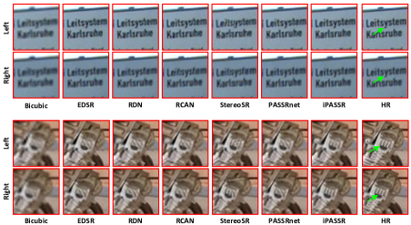
Figure 6: Visual results ($2\times$) achieved by different methods on the KITTI 2015 (top) and Middlebury datasets (bottom).

4.3 Comparison to state-of-the-arts methods

In this section, we compare our iPASSR to several state-of-the-art methods, including four SISR methods , VDSR [8], EDSR [12], RDN [38], RCAN [36]) and three stereo image SR methods (, StereoSR [6], PASSRnet [25], SRRes+SAM [32]). Note that, we retrained all SISR methods [8, 12, 38, 36] on our training set for fair comparison.

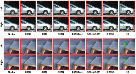
Figure 7: Visual results ($4\times$) achieved by different methods on the KITTI 2015 (top) and Flickr1024 datasets (bottom).

Quantitative results. As shown in Table 4, our iPASSR achieves the highest PSNR and SSIM values on the KITTI 2012 and KITTI 2015 datasets for $2\times$ and $4\times$ SR. For the Middlebury and Flickr1024 datasets, our iPASSR outperforms all stereo image SR methods, but is slightly inferior to EDSR, RDN, and RCAN. Note that, the model sizes of our iPASSR are comparable to PASSRnet but significantly smaller than EDSR, RDN and RCAN. Although a large model enables rich and hierarchical feature representation which can boost the SR performance, we decided to keep our iPASSR lightweight and improve SR performance by exploiting cross-view information in stereo images.

Qualitative results. Qualitative results for $2\times$ and $4\times$ SR are shown in Figs. 6 and 7, respectively. Readers can view this demo video for better comparison. Since input LR images are degraded by the downsampling operation, the SR process is highly ill-posed especially for $4\times$SR. In such cases, SISR methods only use spatial information and cannot well recover the missing details. In contrast, our iPASSR use cross-view information to produce more faithful details with fewer artifacts. Moreover, the images generated by our iPASSR are more stereo-consistent than those generated by PASSRnet and SRRes+SAM.

Figure 8: Visual results achieved by different methods on real-world images [27] for $2\times$SR.

Performance on real-world images. We test the performance of different methods on real-world stereo images by directly applying them to an HR image pair from the Flickr1024 dataset [27]. As shown in Fig. 8, our iPASSR achieves better perceptual quality than the compared methods. It is worth noting that, left and right views of an image pair may suffer different degrees of degradation in real-world cases (e.g., in the region marked by the red box, the left image suffers more severe blurs than the right one). SISR methods cannot well recover the missing details by using the intra-view information only. In contrast, our iPASSR benefits from the cross-view information and produce images with less blurring artifacts.

Table 5: Quantitative results achieved by GwcNet [5] on 4$\times$ SR stereo images. All these metrics were averaged on the test set of the SceneFlow dataset [13], where lower values indicate better performance. Best results are in red and the second best results are blue.

Method	EPE	$>$1px (%)	$>$2px (%)	$>$3px (%)
Bicubic	1.196	11.5	5.96	4.28
VDSR [8]	1.068	10.8	5.37	3.80
PASSRnet [25, 23]	1.019	11.5	5.44	3.72
SRRes+SAM [32]	0.991	11.1	5.18	3.57
iPASSR (ours)	0.949	10.0	4.79	3.35
HR	0.667	6.77	3.34	2.38

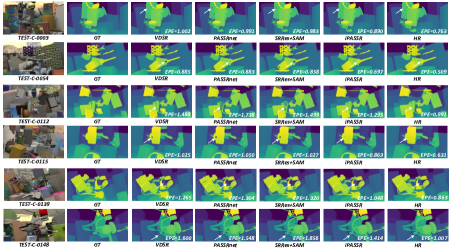
Figure 9: Qualitative results achieved by GwcNet [5] using $4\times$SR stereo images generated by different SR methods.

Benefits to disparity estimation. As stereo-consistent and HR image pairs are beneficial to disparity estimation, we investigate this benefit by using the super-resolved stereo images for disparity estimation. We performed 4$\times$ downsampling on the images from the test sets of the SceneFlow dataset [13], and used different methods to super-resolve these LR images to their original resolution. Then, we applied GwcNet [5] to these super-resolved stereo images for disparity estimation. The original HR images and bicubicly upsampled images were used to produce the upper bound and the baseline results, respectively. End-point-error (EPE) and t-pixel error rate ($>\textit{tpx}$) were used as quantitative metrics to evaluate the estimated disparity. As shown in Table 5, a 0.529 (, $79.3\%$) increase in EPE is introduced when HR input images are replaced with the bicubicly interpolated ones. It demonstrates that the details (e.g., edges and textures) in the stereo images are important to disparity estimation. Note that, our iPASSR can better reduce the error by providing high-quality and stereo-consistent stereo images. The visual examples in Fig 9 demonstrate that the disparity map corresponding to our method is more accurate and close to the one estimated from HR stereo images.

4.4 Discussion

During the retraining of SISR methods, we noticed that the training dataset has an influence on the SR performance. To investigate the influence of training datasets, we used EDSR and RCAN developed on different datasets to perform stereo image SR. As shown in Table 6, EDSR and RCAN achieve better performance when trained on the DIV2K dataset [21]. That is because, the DIV2K dataset was specifically developed for SISR and has higher-quality images than existing stereo image datasets. To demonstrate this claim, we use three no-reference image quality assessment metrics [15, 16, 30] to evaluate the image quality of these datasets. As shown in Table 7, the DIV2K dataset achieves the best results in terms of all the metrics. It demonstrates that high-quality training images can introduce a notable performance gain to deep SR networks.

Table 6: Comparative results achieved by EDSR and RCAN with different training sets for both $2\times$ and $4\times$SR.

Method		KITTI2012	KITTI2015	Middlebury	Flickr1024
EDSR_div2k	2$\times$	31.06/0.925	30.77/0.935	35.34/0.951	28.58/0.909
EDSR_stereo	2$\times$	30.95/0.923	30.73/0.934	34.95/0.949	28.66/0.908
RCAN_div2k	2$\times$	31.16/0.926	30.88/0.945	35.42/0.952	28.64/0.910
RCAN_stereo	2$\times$	31.02/0.923	30.77/0.934	34.90/0.949	28.63/0.908
EDSR_div2k	4$\times$	26.62/0.809	26.39/0.814	29.48/0.842	23.58/0.735
EDSR_stereo	4$\times$	26.35/0.802	26.04/0.804	29.23/0.840	23.46/0.729
RCAN_div2k	4$\times$	26.65/0.809	26.45/0.814	29.56/0.845	23.60/0.737
RCAN_stereo	4$\times$	26.44/0.803	26.22/0.807	29.30/0.840	23.48/0.729

Table 7: No-reference perceptual quality scores of different SR datasets. Both the average value and the standard deviation are reported. Lower scores of BRISQUE [15], NIQE [16] and higher scores of CEIQ [30] indicate better quality.

Dataset	BRISQUE ($\downarrow$)	NIQE ($\downarrow$)	CEIQ ($\uparrow$)
KITTI 2012	17.30 ($\pm$ 6.60)	3.22 ($\pm$0.42)	3.31 ($\pm$0.14)
KITTI 2015	26.41 ($\pm$ 5.26)	3.23 ($\pm$0.48)	3.34 ($\pm$0.19)
Middlebury	14.88 ($\pm$ 9.19)	3.77 ($\pm$0.99)	3.31 ($\pm$0.21)
Flickr1024	19.10 ($\pm$13.57)	3.40 ($\pm$0.99)	3.25 ($\pm$0.36)
DIV2K	11.40 ($\pm$11.98)	2.99 ($\pm$1.05)	3.36 ($\pm$0.30)

5 Conclusion

In this paper, we proposed a method to exploit symmetry cues for stereo image SR. We first proposed a bi-directional parallax attention module (biPAM) and an inline occlusion handling scheme to effectively interact cross-view information, and then equipped biPAM to a Siamese network to develop our iPASSR. Moreover, we proposed several residual losses to achieve robustness to illuminance changes. Extensive ablation studies were performed to validate the effectiveness of our design choices, and comparative results on four public datasets demonstrated the state-of-the-art performance of our method. Furthermore, we made an in-depth analysis on the benefits of stereo image SR to disparity estimation, and the influence of training datasets to image SR.

References

- [1] Kelvin CK Chan, Xintao Wang, Xiangyu Xu, Jinwei Gu, and Chen Change Loy. Glean: Generative latent bank for large-factor image super-resolution. CVPR, 2021.
- [2] Tao Dai, Jianrui Cai, Yongbing Zhang, Shu-Tao Xia, and Lei Zhang. Second-order attention network for single image super-resolution. In CVPR, pages 11065–11074, 2019.
- [3] Chao Dong, Chen Change Loy, Kaiming He, and Xiaoou Tang. Learning a deep convolutional network for image super-resolution. In ECCV, pages 184–199. Springer, 2014.
- [4] Andreas Geiger, Philip Lenz, and Raquel Urtasun. Are we ready for autonomous driving? the kitti vision benchmark suite. In CVPR, 2012.
- [5] Xiaoyang Guo, Kai Yang, Wukui Yang, Xiaogang Wang, and Hongsheng Li. Group-wise correlation stereo network. In CVPR, pages 3273–3282, 2019.
- [6] Daniel S Jeon, Seung-Hwan Baek, Inchang Choi, and Min H Kim. Enhancing the spatial resolution of stereo images using a parallax prior. In CVPR, pages 1721–1730, 2018.
- [7] Sameh Khamis, Sean Fanello, Christoph Rhemann, Adarsh Kowdle, Julien Valentin, and Shahram Izadi. Stereonet: Guided hierarchical refinement for real-time edge-aware depth prediction. In ECCV, pages 573–590, 2018.
- [8] Jiwon Kim, Jung Kwon Lee, and Kyoung Mu Lee. Accurate image super-resolution using very deep convolutional networks. In CVPR, pages 1646–1654, 2016.
- [9] Jiwon Kim, Jung Kwon Lee, and Kyoung Mu Lee. Deeply-recursive convolutional network for image super-resolution. In IEEE Conference on Computer Vision and Pattern Recognition (CVPR), pages 1637–1645, 2016.
- [10] Wei-Sheng Lai, Jia-Bin Huang, Narendra Ahuja, and Ming-Hsuan Yang. Deep laplacian pyramid networks for fast and accurate super-resolution. In CVPR, pages 624–632, 2017.
- [11] Christian Ledig, Lucas Theis, Ferenc Huszár, Jose Caballero, Andrew Cunningham, Alejandro Acosta, Andrew Aitken, Alykhan Tejani, Johannes Totz, Zehan Wang, et al. Photo-realistic single image super-resolution using a generative adversarial network. In CVPR, pages 4681–4690, 2017.
- [12] Bee Lim, Sanghyun Son, Heewon Kim, Seungjun Nah, and Kyoung Mu Lee. Enhanced deep residual networks for single image super-resolution. In CVPRW, pages 136–144, 2017.
- [13] Nikolaus Mayer, Eddy Ilg, Philip Hausser, Philipp Fischer, Daniel Cremers, Alexey Dosovitskiy, and Thomas Brox. A large dataset to train convolutional networks for disparity, optical flow, and scene flow estimation. In CVPR, pages 4040–4048, 2016.
- [14] Moritz Menze and Andreas Geiger. Object scene flow for autonomous vehicles. In CVPR, pages 3061–3070, 2015.
- [15] Anish Mittal, Anush Krishna Moorthy, and Alan Conrad Bovik. No-reference image quality assessment in the spatial domain. IEEE Transactions on Image Processing, 21(12):4695–4708, 2012.
- [16] Anish Mittal, Rajiv Soundararajan, and Alan C Bovik. Making a “completely blind” image quality analyzer. IEEE Signal Processing Letters, 20(3):209–212, 2012.
- [17] Daniel Scharstein, Heiko Hirschmüller, York Kitajima, Greg Krathwohl, Nera Nešić, Xi Wang, and Porter Westling. High-resolution stereo datasets with subpixel-accurate ground truth. In GCPR, pages 31–42. Springer, 2014.
- [18] Wenzhe Shi, Jose Caballero, Ferenc Huszár, Johannes Totz, Andrew P Aitken, Rob Bishop, Daniel Rueckert, and Zehan Wang. Real-time single image and video super-resolution using an efficient sub-pixel convolutional neural network. In CVPR, pages 1874–1883, 2016.
- [19] Wonil Song, Sungil Choi, Somi Jeong, and Kwanghoon Sohn. Stereoscopic image super-resolution with stereo consistent feature. In AAAI, pages 12031–12038, 2020.
- [20] Ying Tai, Jian Yang, and Xiaoming Liu. Image super-resolution via deep recursive residual network. In CVPR, pages 3147–3155, 2017.
- [21] Radu Timofte, Eirikur Agustsson, Luc Van Gool, Ming-Hsuan Yang, and Lei Zhang. Ntire 2017 challenge on single image super-resolution: Methods and results. In CVPRW, pages 114–125, 2017.
- [22] Longguang Wang, Xiaoyu Dong, Yingqian Wang, Xinyi Ying, Zaiping Lin, Wei An, and Yulan Guo. Exploring sparsity in image super-resolution for efficient inference. CVPR, 2021.
- [23] Longguang Wang, Yulan Guo, Yingqian Wang, Zhengfa Liang, Zaiping Lin, Jungang Yang, and Wei An. Parallax attention for unsupervised stereo correspondence learning. IEEE Transactions on Pattern Analysis and Machine Intelligence, 2020.
- [24] Longguang Wang, Yingqian Wang, Xiaoyu Dong, Qingyu Xu, Jungang Yang, Wei An, and Yulan Guo. Unsupervised degradation representation learning for blind super-resolution. CVPR, 2021.
- [25] Longguang Wang, Yingqian Wang, Zhengfa Liang, Zaiping Lin, Jungang Yang, Wei An, and Yulan Guo. Learning parallax attention for stereo image super-resolution. In CVPR, 2019.
- [26] Xintao Wang, Ke Yu, Shixiang Wu, Jinjin Gu, Yihao Liu, Chao Dong, Yu Qiao, and Chen Change Loy. Esrgan: Enhanced super-resolution generative adversarial networks. In ECCVW, pages 0–0, 2018.
- [27] Yingqian Wang, Longguang Wang, Jungang Yang, Wei An, and Yulan Guo. Flickr1024: A large-scale dataset for stereo image super-resolution. In ICCVW, pages 3852–3857, Oct 2019.
- [28] Qingyu Xu, Longguang Wang, Yingqian Wang, Weidong Sheng, and Xinpu Deng. Deep bilateral learning for stereo image super-resolution. IEEE Signal Processing Letters, 2021.
- [29] Bo Yan, Chenxi Ma, Bahetiyaer Bare, Weimin Tan, and Steven C. H. Hoi. Disparity-aware domain adaptation in stereo image restoration. In CVPR, 2020.
- [30] Jia Yan, Jie Li, and Xin Fu. No-reference quality assessment of contrast-distorted images using contrast enhancement. arXiv preprint, 2019.
- [31] Minghao Yin, Zhuliang Yao, Yue Cao, Xiu Li, Zheng Zhang, Stephen Lin, and Han Hu. Disentangled non-local neural networks. In ECCV, 2020.
- [32] Xinyi Ying, Yingqian Wang, Longguang Wang, Weidong Sheng, Wei An, and Yulan Guo. A stereo attention module for stereo image super-resolution. IEEE Signal Processing Letters, 27:496–500, 2020.
- [33] Kai Zhang, Luc Van Gool, and Radu Timofte. Deep unfolding network for image super-resolution. In CVPR, pages 3217–3226, 2020.
- [34] Kai Zhang, Jingyun Liang, Luc Van Gool, and Radu Timofte. Designing a practical degradation model for deep blind image super-resolution. In Arxiv, 2021.
- [35] Kai Zhang, Wangmeng Zuo, and Lei Zhang. Deep plug-and-play super-resolution for arbitrary blur kernels. In CVPR, pages 1671–1681, 2019.
- [36] Yulun Zhang, Kunpeng Li, Kai Li, Lichen Wang, Bineng Zhong, and Yun Fu. Image super-resolution using very deep residual channel attention networks. In ECCV, pages 286–301, 2018.
- [37] Y Zhang, K Li, K Li, B Zhong, and Y Fu. Residual non-local attention networks for image restoration. In ICLR, 2019.
- [38] Yulun Zhang, Yapeng Tian, Yu Kong, Bineng Zhong, and Yun Fu. Residual dense network for image super-resolution. In CVPR, pages 2472–2481, 2018.
- [39] Yulun Zhang, Yapeng Tian, Yu Kong, Bineng Zhong, and Yun Fu. Residual dense network for image restoration. IEEE Transactions on Pattern Analysis and Machine Intelligence, 2020.