A Gap-ETH-Tight Approximation Scheme for Euclidean TSP

We revisit the classic task of finding the shortest tour of $n$ points in $d$-dimensional Euclidean space, for any fixed constant $d\geqslant 2$. We determine the optimal dependence on $\varepsilon$ in the running time of an algorithm that computes a $(1+\varepsilon)$-approximate tour, under a plausible assumption. Specifically, we give an algorithm that runs in $2^{\mathcal{O}(1/\varepsilon^{d-1})}n\log n$ time. This improves the previously smallest dependence on $\varepsilon$ in the running time $(1/\varepsilon)^{\mathcal{O}(1/\varepsilon^{d-1})}n\log n$ of the algorithm by Rao and Smith (STOC 1998). We also show that a $2^{o(1/\varepsilon^{d-1})}\mathrm{poly}(n)$ algorithm would violate the Gap-Exponential Time Hypothesis (Gap-ETH).

Our new algorithm builds upon the celebrated quadtree-based methods initially proposed by Arora (J. ACM 1998), but it adds a new idea that we call sparsity-sensitive patching. On a high level this lets the granularity with which we simplify the tour depend on how sparse it is locally. We demonstrate that our technique extends to other problems, by showing that for Steiner Tree and Rectilinear Steiner Tree it yields the same running time. We complement our results with a matching Gap-ETH lower bound for Rectilinear Steiner Tree.

1 Introduction

The Euclidean Traveling Salesman Problem (Euclidean TSP) is to find a round trip of minimum length for a given set of $n$ points in $d$-dimensional Euclidean space. Its simple statement and clear applicability make the problem very attractive, and work on it has been immensely influential and inspirational. In particular, the Gödel-prize-winning approximation schemes due to Arora [1] and Mitchell [46] are among the most prominent results in approximation algorithms. Because of their elegance, they serve as evergreens in graduate algorithms courses, textbooks on approximation algorithms or optimization [53, 54, 38], and more specialized textbooks [32, 47].

After the publication of these results, an entire research program with many strong results consisting of improvements, generalizations and different applications of the methods from [1, 46] was conducted by many authors (see e.g. the survey [2]). The technique is now known to be useful for a whole host of geometric optimization problems (see the related work paragraph).

The most natural goal within this research direction is to improve the running times to be optimal, i.e. to improve and/or provide evidence that further (significant) improvements do not exist. In the last 25 years only two such results were obtained in $\mathbb{R}^{d}$:

1. Rao and Smith [50] used geometric spanners to improve the $n(\log n)^{\mathcal{O}(1/\varepsilon)^{d-1}}$ time approximation scheme of Arora [1] to run in only $(1/\varepsilon)^{\mathcal{O}(1/\varepsilon)^{d-1}}\cdot n\log n$ time.

2. Bartal and Gottlieb [7] gave a $2^{(1/\varepsilon)^{\mathcal{O}(d)}}\cdot n$ time algorithm in a restricted model of computation. They give a truly linear algorithm in terms of $n$, however the dependence on $\varepsilon$ is worse than the algorithm of Rao and Smith [50].

While these results determine the optimal dependence on $n$, they do not yet settle the much faster growing exponential dependence on $\varepsilon$. This is in contrast with the status of our knowledge of the complexity of many other optimization problems: In the last decade a powerful toolbox for determining (conditionally) optimal exponential running times has been developed.

In the context of TSP in $d$-dimensional Euclidean space (henceforth denoted by $\mathbb{R}^{d}$), this modern research direction culminated in an exact algorithm with running time $2^{\mathcal{O}(n^{1-1/d})}$, which was matched by a lower bound of $2^{\Omega(n^{1-1/d})}$ [19] under the Exponential Time Hypothesis (ETH).

In the context of approximation schemes for TSP, Klein [36] improved algorithms for the unweighted planar case from [28, 3] with a $2^{\mathcal{O}(1/\varepsilon)}n$ time approximation scheme. Subsequently, Marx [45] showed that the dependence on $\varepsilon$ in Klein’s algorithm is conditionally near optimal.The tight exponential dependency of $\varepsilon$ in approximation schemes was also recently obtained in a plethora of other problems, such as Maximum Independent Set in planar graphs [6] and a scheduling problem [14] (see e.g. [24] for a survey).

Given the modern trend of fine-grained algorithm research and the prominence of the discussed approximation schemes for Euclidean TSP, our goal suggests itself:

Goal: Improve the approximation schemes for optimization problems in Euclidean geometry relying on techniques of [1] to have a conditionally optimal running time dependence on $\varepsilon$.

1.1 Our contribution

In this work, we achieve this goal for Euclidean TSP and (Rectilinear) Steiner Tree in $\mathbb{R}^{d}$, and give algorithms with a Gap-ETH-tight dependence on $\varepsilon$.

The running time of our algorithm depends on $T_{\mathrm{spanner}}(n,\varepsilon)$, which is the time needed to compute a light $(1+\varepsilon)$ spanner of $n$ points in $\mathbb{R}^{d}$ (see Section 5 for a more detailed explanation). In most standard models of computation $T_{\mathrm{spanner}}(n,\varepsilon)$ is bounded by $\mathrm{poly}(1/\varepsilon)n\log(n))$. This is a standard representation of the running time and exactly matches the dependence on $n$ of the Rao and Smith algorithm [50]. Our main result reads as follows.

Theorem 1.1 (Main result).

For any integer $d\geqslant 2$ there is a randomized $(1+\varepsilon)$-approximation scheme for Euclidean TSP in $\mathbb{R}^{d}$ that runs in $2^{\mathcal{O}(1/\varepsilon)^{d-1}}n+T_{\mathrm{spanner}}(n,\varepsilon)$ time. Moreover, this cannot be improved to a $2^{o((1/\varepsilon)^{d-1})}\cdot\mathrm{poly}(n)$ time algorithm, unless Gap-ETH fails.

Thus, we improve the previously best $(1/\varepsilon)^{\mathcal{O}(1/\varepsilon)^{d-1}}$ dependence of $\varepsilon$ in the running time of [50] to $2^{\mathcal{O}(1/\varepsilon)^{d-1}}$. Note that here and in the sequel our big-$\mathcal{O}$ notation hides factors that depend only on $d$ since it is assumed to be constant. Our running times are double exponential in the dimension $d$, which is expected because of Trevisan’s lower bound [52].

Theorem 1.1 improves the running time dependence on $\varepsilon$ all the way to conditional optimality: we show that an EPTAS with an asymptotically better dependence on $\varepsilon$ in the exponent is not possible under Gap-ETH, for constant dimension $d$. Note that our algorithms can be derandomized at the cost of an extra $n^{d}$ factor in the running time, which maintains conditional optimality in terms of $\varepsilon$.

Our lower bound for Euclidean TSP is derived from a construction for Hamiltonian Cycle in grid graphs [20] in combination with Gap-ETH [22, 44] (see Section 6).

Our new algorithmic techniques enable us to improve approximation schemes for another fundamental geometric optimization problem: the Rectilinear Steiner Tree and Euclidean Steiner Tree problems.

Theorem 1.2.

For any integer $d\geqslant 2$ there is a randomized $(1+\varepsilon)$-approximation scheme for Euclidean Steiner Tree and Rectilinear Steiner Tree in $\mathbb{R}^{d}$ that runs in $2^{\mathcal{O}(1/\varepsilon)^{d-1}}n+T_{\mathrm{spanner}}(n,\varepsilon)$ time.⁶ Moreover, the algorithm for Rectilinear Steiner Tree cannot be improved to a $2^{o((1/\varepsilon)^{d-1})}\cdot\mathrm{poly}(n)$ time algorithm, unless Gap-ETH fails.

This directly improves state-of-the-art algorithms by Rao and Smith [50] and Bartal and Gottlieb [27] in all regime of parameters $n$ and $\varepsilon$. We complement our results with a matching lower bound for Rectilinear Steiner Tree.

The lower bound for Rectilinear Steiner Tree requires new ideas since there is no known ETH-based lower bound for the exact version of the problem. Our construction is based on a reduction from Grid Embedded Connected Vertex Cover from [20] and combination of gadgets proposed by [26] (see Section 6). We leave it as an open problem to give a matching lower bound on our algorithm for Euclidean Steiner Tree.

1.2 The existing approximation schemes and their limitations

The approximation scheme from Arora [1] serves as the basis of our algorithm and we assume that the reader is familiar with its basics (see [54, 53] for a comprehensive introduction to the approximation scheme). In this section we consider $d=2$ for simplicity.

In a nutshell, Arora’s strategy in the plane is first to move the points to the nearest grid points in an $L\times L$ grid where $L=\mathcal{O}(n/\varepsilon)$. This grid is subdivided using a hierarchical decomposition into smaller squares (a quadtree, see definition in Section 2), where on each side of a square $\mathcal{O}((\log n)/\varepsilon)$ equidistant portals are placed. Arora proves a structure theorem, which states that there is a tour of length at most $(1+\varepsilon)$ times the optimal tour length that crosses each square boundary $\mathcal{O}(1/\varepsilon)$ times, and only through portals. This structure theorem is based on a patching procedure, which iterates through the cells of the quadtree (starting at the smallest cells) and patches the tour such that the resulting tour crosses all cell boundaries only $\mathcal{O}(1/\varepsilon)$ times and only at portals, and it does it in such a way that the new tour is only slightly longer. While such a promised slightly longer tour does not necessarily exist for a fixed quadtree, a randomly shifted quadtree works with high probability. The algorithm thus proceeds by picking a randomly shifted quadtree, and by performing a dynamic programming algorithm on progressively larger squares and the bounded set of possibilities in it to find a patched tour.

The first improvement to Arora’s algorithm was achieved by Rao and Smith [50] (see [47, Chapter 16] for a modern description of their methods). Recall that Arora placed equidistant portals. Rao and Smith’s idea is to use light spanners to “guide” the approximate TSP tour and select portals on the boundary not uniformly. They show that it is sufficient to look for the shortest tour within a spanner, or more precisely, they patch the given spanner such that the resulting graph has $1/\varepsilon^{\mathcal{O}(1)}$ crossings with each quadtree cell, while still containing a $(1+\varepsilon)$-approximate tour. Similarly to Arora’s algorithm, it is sufficient to consider tours that cross each square boundary $\mathcal{O}(1/\varepsilon)$ times, but now the number of portals is $(1/\varepsilon)^{\mathcal{O}(1)}$. Consequently, the algorithm of Rao and Smith needs only $\left((1/\varepsilon)^{\mathcal{O}(1)}\right)^{\mathcal{O}(1/\varepsilon)}=2^{\mathcal{O}((1/\varepsilon)\cdot\log(1/\varepsilon))}$ subsets of portals to consider for each square in their corresponding dynamic programming algorithm.

Why do known techniques fail to get a better running time?

To get the dependence on $\varepsilon$ in the running time down to $2^{\mathcal{O}(1/\varepsilon)}$, the bottleneck is to get the number of candidate sets of where the tour crosses a cell boundary down to $2^{\mathcal{O}(1/\varepsilon)}$.

One could hope to improve Arora’s algorithm by decreasing the number of portals from $\mathcal{O}(\log n/\varepsilon)$ to $\mathcal{O}(1/\varepsilon)$, but this is not possible: the structure theorem would fail even if the optimal tour is a rotated square (with $n-4$ input points on its sides).

Another potential approach would be to improve the spanners and the spanner modification technique of Rao and Smith to get a graph that contains a $(1+\varepsilon)$-approximate tour, while having only $\mathcal{O}(1/\varepsilon)$ crossings on each side of each square. Such an improvement seems difficult to accomplish as even with Euclidean Spanners [41] of optimal lightness or the more general Euclidean Steiner Spanners [42]. Le and Solomon [41] gave a lower bound of $\tilde{\Omega}(1/\varepsilon)$ on the lightness of Euclidean Steiner Spanners in $d=2$, which was matched very recently by Bhore and Tóth [9]. Even with that optimal Steiner spanner, the patching method of Rao and Smith yields a guarantee of only $\widetilde{\mathcal{O}}(1/\varepsilon^{2})$ crossings per square and it is not clear if one can even get $\mathcal{O}(1/\varepsilon^{1.99})$ potential crossings per square.

1.3 Our technique: Sparsity-Sensitive Patching

We introduce a new patching procedure. Slightly oversimplifying and still focusing on $2$ dimensions, it iterates over the cells of the quadtree like Arora, but it processes a cell boundary as follows: Sparsity-Sensitive Patching: For a cell boundary that is crossed by a tour at $1<k\leqslant\mathcal{O}(1/\varepsilon)$ crossings, modify the tour by mapping each crossing to the nearest portal from the set of $g$ equidistant portals. Here $g$ is a granularity parameter that depends on $k$ as $g=\Theta(1/(\varepsilon^{2}k))$. This can be used in combination with dynamic programming to prove Theorem 1.1 since it produces a tour for which the number of possibilities for the set of crossings of the tour with a cell boundary is $\sum_{k}\binom{\mathcal{O}(1/(\varepsilon^{2}k))}{k}=2^{\mathcal{O}(1/\varepsilon)}$ (see Claim 3.4).

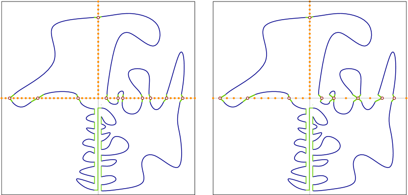
Figure 1: On neighboring cells of the quadtree, one must ensure that the tour crosses at most $1/\varepsilon$ times, chosen from a limited set of portals. Left: Arora’s structure theorem snaps the tour to one of $\mathcal{O}(\frac{\log n}{\varepsilon})$ equally spaced portals. Right: The number of possible portal locations depends on the number of crossings; the fewer portals are used, the more precisely they are chosen. Both techniques use the Patching Lemma between the bottom two cells as their shared boundary is crossed more than $1/\varepsilon$ times.

Bounding the patching cost.

Seemingly, our Sparsity-Sensitive procedure appears to be quite similar to Arora’s procedure, so one may wonder why the previous improvements to Arora’s procedure overlooked it. The reason is because it is slightly counter-intuitive (to increase precision when the tour is already sparse), and it requires a subtle analysis of the patching cost. This proof is the main contribution of this paper.

We will informally describe how we do this next. Similarly to the patching cost analysis of Arora’s patching procedure, our starting point is that the total number of crossings that an optimal tour $\pi$ will have with all horizontal (and vertical) lines aligned at integer coordinates is proportional to the total weight of the tour (Lemma 2.2). Since we can afford an additional cost of $\varepsilon\cdot\mathrm{wt}(\pi)$, it is enough to show that each such crossing incurs (in an amortized sense) at most $\mathcal{O}(\varepsilon)$ patching cost.

Let $\text{PC}(k,\ell)$ be the patching cost of a horizontal quadtree-cell side of length $\ell$ with $k$ crossings. Since we connect each crossing to a portal that is of distance at most $\ell/g$, and the total patching cost is never greater than $\mathcal{O}(\ell)$ (since we can just “buy” an entire line), we obtain $\text{PC}(k,\ell)\leqslant\mathcal{O}(\min\{\ell,k\ell/g\})$. The amortized patching cost per crossing is then

$$\frac{\text{PC}(k,\ell)}{k}=\mathcal{O}\left(\frac{\min\{\ell,k\frac{\ell}{g}\}}{k}\right)=\mathcal{O}\left(\frac{\ell}{k}\min\{1,(k\varepsilon)^{2}\}\right),$$ (1)

and this is maximized when $k=1/\varepsilon$, for which it is $\varepsilon\ell$.

Because we consider a random shift of the quadtree, a crossing of $\pi$ with a fixed horizontal line $h$ will end up in a cell side of length $L/2^{i}$ with probability at most $2^{i-1}/L$, for each $0\leqslant i\leqslant\log L$ (Lemma 2.3). Letting $\alpha_{i}(x)$ be the (amortized) patching cost due to the crossing $x$ on line $h$ if $h$ has level $i$, $x$ incurs

$$\sum_{i=0}^{\log L}\frac{2^{i-1}}{L}\cdot\alpha_{i}(x)$$ (2)

amortized patching cost in expectation. Naively applying (1) for each $i$ to get $\alpha_{i}\leqslant\varepsilon L/2^{i}$ and putting this bound into (2), gives an undesirably high cost of $\mathcal{O}(\varepsilon\log L)$.

To get this cost down to $\mathcal{O}(\varepsilon)$, we need to use a more refined argument. Intuitively, we exploit that in the worst case the bound $\alpha_{i}(x)\leqslant\varepsilon L/2^{i}$ is tight only for a single $i=i^{*}$. Subsequently, we show that for levels above and below $i^{*}$ we have a geometrically decreasing series of costs, which will show that the cost in (2) is bounded by $\mathcal{O}(\varepsilon)$. In our proof we formalize this with a charging scheme based on the distance of the crossing to the next crossing on the horizontal line.

1.4 More related work

The framework of Arora [1] and Mitchell [46] was employed for several other optimization problems in Euclidean space such as Steiner Forest [11], $k$-Connectivity [16], $k$-Median [37, 5], Survivable Network Design [17]. We hope our techniques will also find some applications in them.

The original results from [1, 46] was also applied or generalized to different settings. The state-of-the-art for the Traveling Salesman Problem in planar graphs is now very similar to the Euclidean case. [29] gave the first PTAS for TSP in planar graphs, which was later extended by [4] to weighted planar graphs. Klein [36] proposed a $2^{\mathcal{O}(1/\varepsilon)}n$ time approximation scheme for TSP in unweighted planar graphs, which later was proven by Marx [45] to be optimal assuming ETH. Klein [35] also studied a weighted subset version of TSP that generalizes the planar Euclidean case and gave a PTAS for the problem.

The literature then generalized the metrics much further. Without attempting to give a full overview, some prominent examples are the algorithms in minor free graphs [21, 12, 40], algorithms in doubling metrics [8, 13], and algorithms in negatively curved spaces [39], each of which is at least inspired by the result of Arora [1] and Mitchell [46].

Recently, Gottlieb and Bartal [27] gave a PTAS for Steiner Tree in doubling metrics. Moreover, they proposed a $2^{(1/\varepsilon)^{\mathcal{O}(d^{2})}}n\log{n}$ time algorithm for Steiner Tree in $d$-dimensional Euclidean Space with a novel construction of banyan.

There is also a vast literature concerning Euclidean Spanners (see the book [47] for an overview). Very recently Le and Solomon [41] proved that greedy spanners are optimal and in [42] they gave a novel construction of light Euclidean Spanners with Steiner points. Many such results mention approximation schemes for Euclidean TSP as a major motivation.

1.5 Organization

This paper is organized as follows. In Section 2 we define the building blocks of Arora’s approach that we use. Next in Section 3 we state our structural theorem, and informally prove Theorem 3.1. Section 4 proves the Structure Theorem, and in Section 5.1 we show how to use it in combination with dynamic programming to establish the algorithmic parts of Theorem 1.1 and Theorem 1.2. In Section 6 the matching lower bounds are presented, and in Section 7 we conclude the paper.

2 Introduction to Arora’s Technique

2.1 Ingredients from Arora’s approach

In the following we assume an instance of Euclidean TSP is given by a point set $P\subseteq\mathbb{R}^{d}$. By using a standard $\mathcal{O}(n\log n)$ time perturbation step as preprocessing (see e.g. [47, Section 19.2]), we may assume that $P\subseteq\{0,\ldots,L\}^{d}$ for some integer $L=\mathcal{O}(n\sqrt{d}/\varepsilon)$ that is a power of $2$.

A salesman path will be a closed path that visits all points from $P$ but may make some digressions. The following folklore lemma, is typically used to reduce the number of ways a salesman path can cross a given hyperplane.

Lemma 2.1 (Patching Lemma [1]).

Let $h$ be a hyperplane, $\pi$ be a closed path, and $I(\pi,h)$ be the set of intersection of $\pi$ with $h$. Suppose $T$ be a tree that spans $I(\pi,h)$. Then, for any point $p$ in $T$ there exist line segments contained in $h$ whose total length is at most $\mathcal{O}(\mathrm{wt}(T))$ and whose addition to $\pi$ changes it into a closed path that crosses $I(\pi,h)$ at most twice and only at $p$.

Dissection and Quadtree.

Now we introduce a commonly used hierarchy to decompose $\mathbb{R}^{d}$ that will be instrumental to guide our algorithm. Pick $a_{1},\ldots,a_{d}\in\{1,\ldots,L\}$ independently and uniformly at random and define $\mathbf{a}:=(a_{1},\ldots,a_{d})$. Consider the hypercube

$$C(\mathbf{a}):=\bigtimes_{i=1}^{d}[-a_{i}+1/2,\,2L-a_{i}+1/2].$$

Note that $C(\mathbf{a})$ has side length $2L$ and each point from $P$ is contained in $C(\mathbf{a})$ by the assumption $P\subseteq\{0,\ldots,L\}^{d}$.

Let the dissection $D(\mathbf{a})$ of $C(\mathbf{a})$ to be the tree $T$ that is recursively defined as follows: With each vertex of $T$ we associate a hypercube in $\mathbb{R}^{d}$. For the root of $T$ this is $C(\mathbf{a})$ and for the leaves of $T$ this is a hypercube of unit length. Each non-leaf vertex $v$ of $T$ with associated hypercube $\bigtimes_{i=1}^{d}[l_{i},u_{i}]$ has $2^{d}$ children with which we associate $\bigtimes_{i=1}^{d}I_{i}$, where $I_{i}$ is either $[l_{i},(l_{i}+u_{i})/2]$ or $[(l_{i}+u_{i})/2,u_{i}]$. We refer to such a hypercube that is associated with a vertex in the dissection as a cell of the dissection.

The quadtree $QT(P,\mathbf{a})$ is obtained from $D(\mathbf{a})$ by stopping the subdivision whenever a cell has at most $1$ point from the input point set $P$. This way, every cell is either a leaf that contains $0$ or $1$ input points, or it is an internal vertex of the tree with $2^{d}$ children, and the corresponding cell contains at least $2$ input points. We say that a cell $C$ is redundant if it has a child that contains the same set of input points as the parent of $C$. A redundant path is a maximal ancestor-descendant path in the tree whose internal vertices are redundant. The compressed quadtree $\mathrm{CQT}(P,\mathbf{a})$ is obtained from $QT(P,\mathbf{a})$ by removing all the empty children of redundant cells, and replacing the redundant paths with edges. In the resulting tree some internal cells may have a single child; we call these compressed cells. It is well-known and easy to check that compressed quadtrees have $\mathcal{O}(n)$ vertices.

A grid hyperplane is a point set of the form $\{(x_{1},\ldots,x_{d}:x_{i}=1/2+j)\}$ for some integer $j$. For a set of line segments $S$ we define $I(S,h)$ as the set of line segments from $S$ that cross $h$. Note that for every face $F$ of every cell in $D(\mathbf{a})$, there is a unique grid hyperplane that contains $F$.

The following simple lemma relates the number of crossings with grid hyperplanes with the total length of the line segments.

Lemma 2.2 (c.f., Lemma 19.4.1 in [47]).

If $S$ is a set of line segments in $\mathbb{R}^{d}$, then

$$\sum_{h\text{:grid hyperplane}}|I(S,h)|\leqslant\sqrt{d}\cdot\mathrm{wt}(S)$$

For a grid hyperplane $h$ we define the level of $h$ to be the smallest integer $i$ such that $D(\mathbf{a})$ contains a cell with sides of length $2L/2^{i}$, one of whose faces is contained in $h$.

Lemma 2.3 (Lemma 19.4.3 [47]).

Let $h$ be a grid hyperplane, and let $i$ be an integer satisfying $0\leqslant i<1+\log L$. Then the probability that the level of $h$ is equal to $i$ is at most $2^{i-1}/L$.

2.2 The patching procedure of Arora

We now briefly describe the building blocks from [1], because it will be useful to contrast it to our new approach.

Definition 2.4 ($m$-regular set).

An $m$-regular set of portals on a $d$-dimensional hypercube $C$ is an orthogonal lattice $\mathrm{grid}(C,m)$ of $m$ points in the cube. Thus, if the cube has side length $\ell$, then the spacing between the portals is $\ell/m^{1/d}$.

Definition 2.5 ($r$-light).

A set of line segments $S$ is $r$-light with respect to the dissection $D(\mathbf{a})$ if it crosses each face of each cell of $D(\mathbf{a})$ at most $r$ times.

Theorem 2.6 (Arora’s Structure Theorem).

Let $P\subseteq\{0,\ldots,L\}^{d}$, and let $\mathrm{wt}(OPT)$ be the minimum length of a salesman tour visiting $P$. Let the shift vector $\mathbf{a}$ be picked randomly. Then with probability at least $1/2$, there is a salesman path of cost at most $(1+\varepsilon)\mathrm{wt}(OPT)$ that is $r$-light with respect to $D(\mathbf{a})$ such that it crosses each facet $F$ of a cell of $D(\mathbf{a})$ only at points from $\mathrm{grid}(F,m)$, for some $m=(\mathcal{O}((\sqrt{d}/\varepsilon)\log L))^{d-1}$ and $r=(\mathcal{O}(\sqrt{d}/\varepsilon))^{d-1}$.

3 Overview of our methods

In this section we sketch the proof of our main result in the case of $d=2$ (and from now on we focus on $d=2$ unless stated otherwise).

Theorem 3.1.

There is a randomized $(1+\varepsilon)$-approximation scheme that solves Euclidean TSP in two dimensions in $2^{\mathcal{O}(1/\varepsilon)}n\,\textup{polylog}(n)$ time.

For simplicity in this section we focus on an algorithm with a slightly worse dependence on $n$. In Section 5 we will provide an algorithm that matches the $n$-dependence of the algorithm by Rao and Smith [50].

Before we begin, let us discus how Arora [1] uses his structure theorem and the bottlenecks of his approach. The algorithmic usefulness of Theorem 2.6 lies in the fact that the promised tour can be found relatively quickly with a dynamic programming algorithm. The table entries are indexed by a cell of $\mathrm{CQT}(P,\mathbf{a})$ and all possible ways the tour can enter and leave the cell. The number of such possibilities is $\binom{m}{r}2^{\mathcal{O}(r)}$, which is roughly $(\log n)^{\mathcal{O}(1/\varepsilon)}n$.

The proof of Theorem 2.6 (and its later extensions) uses a so-called patching procedure that modifies an (optimal) tour to a tour with the desired properties, but without increasing the length by too much. For example, for Theorem 2.6 a patching procedure iterates over each quadtree edge $F$ and rewires each crossing to a “portal” from $\mathrm{grid}(F,m)$.

Such patching procedures can be analyzed via bounding the expected cost $\mathrm{cost}(h)$ of the crossings of the tour with a fixed hyperplane $h$. By Lemma 2.2, it is sufficient to show that a fixed crossing point on $h$ incurs only $\mathcal{O}(\varepsilon)$ cost. The analysis of the above patching procedure for proving Theorem 2.6 in two dimensions is relatively direct since the connection to a point from $\mathrm{grid}(F,m)$ costs $\mathcal{O}(L/(2^{i}m))$ and the probability that $h$ gets level $i$ is $2^{i-1}/L$ by Lemma 2.3.

To ensure $r$-lightness, one can use the following patching procedure: Let us assume for simplicity that $h$ is a horizontal line, and $c_{1}<c_{2}<\ldots<c_{k}$ are the $x$-coordinates of the $k=|I(G,h)|$ crossings. Define the proximity of the $j$-th crossing as $\mathrm{pro}(c_{j})=c_{j}-c_{j-1}$ (for $j=1$, use $c_{0}=-\infty$). The patching procedure works as follows: If $\mathrm{pro}(c_{j})\leqslant\frac{L}{2^{i}r}$ then connect $c_{j}$ to $c_{j-1}$, and run Lemma 2.1 on the obtained components to reroute all connections. It is easy to see that the obtained tour is $r$-light since each cell boundary contained in $h$ is of length $L/2^{i}$ and thus contains at most $r$ points with proximity more than $L/(2^{i}r)$. To see that the total length of the added connections is at most $|I(\pi,h)|/r$, note that a single crossing $x$ incurs patching cost at most

$$\sum_{i=0}^{\log L}\frac{2^{i-1}}{L}\left[\mathrm{pro}(x)\leqslant\frac{L}{2^{i}\cdot r}\right]\mathrm{pro}(x)=\sum_{i=0}^{\theta}\frac{2^{i-1}}{L}\mathrm{pro}(x)\leqslant\frac{2^{\theta}}{L}\mathrm{pro}(x)\leqslant\frac{1}{r},$$ (3)

where the brackets denote an indicator function and $\theta:=\log\left(\frac{L}{r\cdot\mathrm{pro}(x)}\right)$.

3.1 Our Structure Theorem

Now we present and discuss the main structure theorem that allows us to prove Theorem 1.1. We state the theorem for a general dimension $d$, but in the interest of simplicity, in this section we only sketch the proof for $d=2$.

Definition 3.2 ($r$-simple salesman tour).

A tour $\pi$ in $\mathbb{R}^{d}$ is $r$-simple if for every face $F$ of every cell in $D(\mathbf{a})$, either

1. $\pi$ crosses $F$ at only one point, or

2. $\pi$ crosses $F$ at most $m$ times, and only at points from $\mathrm{grid}(F,g)$, for $g\leqslant r^{2d-2}/m$.

Moreover, for any point $p$ on a hyperplane $h$, $\pi^{\prime}$ can cross $h$ at most twice via $p$.

Note that $m\leqslant 2g$ since each portal from $\mathrm{grid}(F,g)$ is visited at most twice, and therefore it holds that $m\leqslant 2r^{d-1}$.

Theorem 3.3 (Structure Theorem).

Let $\mathbf{a}$ be a random shift and let $\pi$ be a salesman path that visits $P\subseteq\mathbb{R}^{d}$. For any large enough integer $r$ there is an $r$-simple salesman path $\pi^{\prime}$ visiting $P$ such that both

1. $\mathbb{E}_{\mathbf{a}}[\mathrm{wt}(\pi^{\prime})-\mathrm{wt}(\pi)]\leqslant\mathcal{O}(d^{2}\cdot\mathrm{wt}(\pi)/r)$, and

2. if $\pi$ crosses a facet $F$ of a hypercube of $D(\mathbf{a})$ at only one point, then $\pi^{\prime}$ crosses $F$ at the same point.

Theorem 3.3 is the main contribution of this paper. Before we sketch its proof, let us informally describe how our Structure Theorem can be used to prove Theorem 3.1 if $d=2$. We set $r=\mathcal{O}(1/\varepsilon)$. If we find an $r$-simple tour of lowest weight, then property (i) of Theorem 3.3 guarantees that this tour is a $(1+\varepsilon)$-approximation of an optimal TSP. Similarly to Arora [1] we can use dynamic programming to find such a tour. The number of possible ways in which the tour can enter and leave a cell of the quadtree is at most $\binom{\mathcal{O}(1/(\varepsilon^{2}m))}{m}2^{\mathcal{O}(m)}\cdot\mathrm{poly}(n)$, since there are at most $\mathrm{poly}(n)$ possibilities for the location of crossing if there is at most one crossing.⁹ The number of table entries can then be upper bounded with $2^{\mathcal{O}(1/\varepsilon)}\mathrm{poly}(n)$ via the following claim:

Claim 3.4.

For every $1\leqslant a\leqslant b$, it holds that $\binom{b/a}{a}\leqslant e^{\sqrt{b/e}}$.

Proof.

If $a>\sqrt{b}$, then $\binom{b/a}{a}=0$ and the inequality follows. If $a\leqslant\sqrt{b}$, then by the standard upper bound $\binom{n}{k}\leqslant(\frac{n\cdot e}{k})^{k}$ we have that $\binom{b/a}{a}\leqslant\left(\frac{b\cdot e}{a^{2}}\right)^{a}$. In the interval $a\in[1,\sqrt{b}]$, the latter expression is maximized for $a=\sqrt{b/e}$, where it equals $e^{\sqrt{b/e}}$. ∎

To get the $\mathrm{poly}(n)$ factor in the running time down to $\,\textup{polylog}(n)$, note that we can first apply Theorem 2.6 with smaller $\varepsilon$ to ensure there are $\log^{\mathcal{O}(1)}(n)$ possibilities for the case where the tour crosses a cell edge at a single point.

Theorem 3.1 now follows from the correctness of our Structure Theorem.

3.2 Intuition behind Sparsity-Sensitive Patching

Now we describe on an intuitive level how Theorem 3.3 is established in $\mathbb{R}^{2}$; a formal proof of the general version is postponed to Section 4. From the analysis of Subsection 2.2, and in particular (3), it appears that crossings in a cell with at least $r$ crossings contribute only $\mathcal{O}(1/r)$ to the expected patching cost (note that in the algorithm we set $r=\mathcal{O}(1/\varepsilon)$). We must keep the number of possible ways in which the tour can cross a cell of the dissection to $2^{\mathcal{O}(r)}$, but we also need to decrease the patching cost significantly in case of fewer than $r$ crossings.

Our Sparsity-Sensitive Patching achieves this by taking each cell $C$ of the dissection and each side $F$ of $C$ with at least two crossings, and connecting each crossing $x$ on $F$ as follows (see Figure 2).

1. Let $N$ be the set of “near” crossings, that is, $N$ is the set of crossings of $\pi$ and $F$ satisfying $\mathrm{pro}(x)\leqslant\frac{L}{2^{i}r}$, where $i$ is the level of the line of $F$ in the dissection.

2. Let $G$ be the set of remaining crossings of $\pi$ with $F$.

3. Create a set of line segments $T^{\prime}_{F}$ by connecting each vertex from $N$ to its successor and, if $|G|>1$, connecting each vertex from $G$ to the closest point in $\mathrm{grid}(F,r^{2}/|G|)$.

4. Apply Lemma 2.1 to each set of touching line segments of $T^{\prime}_{F}$ to obtain a new tour $\pi^{\prime}$ that crosses $F$ only at $|G|$ points of $\mathrm{grid}(F,r^{2}/|G|)$, and at most twice at each of these points.

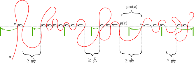
Figure 2: Construction of a set of line segments $T^{\prime}_{F}$ in $d=2$. The tour $\pi$ is colored red. Green portals denote the points in $\mathrm{grid}(F,r^{2}/|G|)$. The leftmost point and the points with $\mathrm{pro}(x)>L/(2^{i}/r)$ form the set $G$ and are connected to the closest portal from the grid by a green arrow. Points with $\mathrm{pro}(x)\leqslant L/(2^{i}r)$ form the set $N$ and they are connected to their parent with black arrows. The set of line segments $T^{\prime}_{F}$ is indicated with a collection of black and green arrows.

Note that if $|G|=1$, then we do not guarantee that the single crossing is in $\mathrm{grid}(F,r^{2}/|G|)$ (and this is also not promised in Theorem 2.1). The reason that we do this is that the one crossing in $G$ may have arbitrary large proximity, and the proximity of all other crossings can be arbitrarily small, and therefore we cannot ‘charge’ the patching cost to a vertex in the analysis that follows. Therefore we can focus on $|G|>1$.

Similarly to Subsection 2.2, we bound the expected patching cost that a single patching incurs in terms of its proximity. By Lemma 2.1 the increase of $\pi^{\prime}$ is proportional to $\mathrm{wt}(T^{\prime}_{F})$. Since each of the connections at Step $3$ are of length at most $\frac{L|G|}{2^{i}r^{2}}$, we have

$$\mathrm{wt}(T^{\prime}_{F})\leqslant\sum_{x\in N}\mathrm{pro}(x)+\sum_{x\in G}\frac{L|G|}{2^{i}r^{2}}\leqslant\sum_{x\in N}\mathrm{pro}(x)+\frac{L|G|^{2}}{2^{i}r^{2}},$$ (4)

so we need to bound $|G|^{2}$ in terms of the proximities of the vertices in $G$. Let $\rho$ denote the crossing with the minimum $x$-coordinate. Thus $\sum_{x\in G\setminus\{\rho\}}\mathrm{pro}(x)\leqslant L/2^{i}$ since all crossings in $G$ are in an interval of length $L/2^{i}$. By Cauchy-Schwartz, we therefore have that

$$|G\setminus\{\rho\}|^{2}\leqslant\left(\sum_{x\in G\setminus\{\rho\}}\mathrm{pro}(x)\right)\left(\sum_{x\in G}\frac{1}{\mathrm{pro}(x)}\right)\leqslant\frac{L}{2^{i}}\sum_{x\in G}\frac{1}{\mathrm{pro}(x)}.$$ (5)

and combining with (4) gives that

$$\mathrm{wt}(T^{\prime}_{F})\leqslant\sum_{x\in N}\mathrm{pro}(x)+\left(\frac{L}{2^{i}r}\right)^{2}\sum_{x\in G}\frac{1}{\mathrm{pro}(x)}.$$

Next, for a fixed line $h$ of level $i$ we attribute the cost to the crossing $x\in I(\pi,h)$ as follows. If $x\in N$, then the cost of the crossing $x\in I(\pi,h)$ is $\alpha_{i}(x):=\mathrm{pro}(x)$. Otherwise if $x\in G$, the cost is $\alpha_{i}(x):=(\frac{L}{2^{i}r})^{2}\frac{1}{\mathrm{pro}(x)}$. Now, for a fixed grid line $h$ and $x\in I(\pi,h)$ the expected patching cost due to $x$ is:

$$\sum_{i=0}^{\log L}\Pr[h\text{ has level }i]\cdot\alpha_{i}(x)=\mathcal{O}\left(\sum_{i=0}^{\theta}\frac{2^{i}}{L}\mathrm{pro}(x)+\sum_{i=\theta+1}^{\log L}\frac{L}{2^{i}}\frac{1}{r^{2}\mathrm{pro}(x)}\right),$$

where $\theta:=\log\frac{L}{r\cdot\mathrm{pro}(x)}$ (recall that $x\in G$ when $\mathrm{pro}(x)>\frac{L}{2^{i}r}$ and $x\in N$ otherwise). The right hand side is at most $\mathcal{O}(1/r)$ by the convergence of sums of geometric progressions. Thus the total patching cost is at most

$$\sum_{h}\sum_{x\in I(\pi,h)}\sum_{i=0}^{\log L}\Pr[h\text{ has level }i]\cdot\alpha_{i}(x)\leqslant\sum_{h}\mathcal{O}(|I(\pi,h)|/r)\leqslant\mathcal{O}(\mathrm{wt}(\pi)/r)$$

by Lemma 2.2, as required.

4 The proof of the Structure Theorem in $\mathbb{R}^{d}$

In this section we formally prove the Structure Theorem in $d$-dimensional Euclidean space. Before we prove it, we first show the existence of a certain ‘base-line tree’ in $d$-dimensional Euclidean space. This tree will be a subset of a hyperplane and parts of it will be used via the invocation of the patching routine from Lemma 2.1 to reduce the number of crossings of the tour with the hyperplane. In $\mathbb{R}^{2}$, this tree is just an entire line segment, but in higher dimensions this is less direct. Similar trees were also used for the case $d>2$ by a previous algorithm (see [50]), but we use it in a slightly different way. Crucially, the base-line tree determines the proximities of the crossings and whether a given crossing point will be connected to a point from a grid or not.

4.1 The base-line tree

The following Lemma is based on [47, Lemma 19.5.1]. There are however two important differences. First, we do not need an efficient construction and only need to prove the existence of such a tree $T$. Second, [47, Lemma 19.5.1] does not guarantee a property (b) in Lemma 4.1.

Lemma 4.1.

Let $D(\mathbf{a})$ be a dissection in $\mathbb{R}^{d}$. Then there is a tree $T$ of $V$ such that

1. $T$ is $1$-light with respect to $D(\mathbf{a})$, and

2. for each cell $C$ of the dissection $D(\mathbf{a})$ with side-length $\ell$ and $Q\subseteq C$, it holds that the subtree $T^{\prime}$ of $T$ that spans $Q$ satisfies $\mathrm{wt}(T^{\prime})\leqslant 4d\ell|Q|^{1-1/d}$.

Proof.

For convenience we extend the dissection $D(\mathbf{a})$ to an infinite dissection $D^{\prime}(\mathbf{a})$ as follows: For an infinite number of iterations, each smallest hypercube is split into $2^{d}$ axis-parallel smaller hypercubes of equal size in the unique way.

The construction of $T$ is as follows. For a hypercube $C$ in the dissection $D^{\prime}(\mathbf{a})$ we define the skeleton of $C$ to be the graph whose vertex set consists of the $2^{d}$ corners of $C$ and whose edge set consists of the $d2^{d-1}$ edges of $C$. We define $\mathrm{cor}(C)$ to be the corner of $C$ of which all coordinates are the smallest possible. We construct a tree $T$ that only crosses each $C$ of the dissection at $\mathrm{cor}(C)$. To do so, for each $C$ we add a spanning tree of the skeleton of $C$ rooted at $\mathrm{cor}(C)$ with depth at most $d$; this tree is denoted by $T_{C}$. Note that different trees $T_{C}$ have overlaps. The cell $C$ has a unique child $C^{\star}$ where $\mathrm{cor}(C)=\mathrm{cor}(C^{\star})$; we identify these root points in $T_{C}$ and $T_{C^{\star}}$. If $C^{\prime}\neq C^{\star}$ is a child of $C$, then we identify the root of $T_{C^{\prime}}$ and the same point in $T_{C^{\star}}$. The result is a tree $T$ (with overlaps) that spans all vertices of all cells in $D^{\prime}(\mathbf{a})$.

By construction, the tree $T$ only crosses each cell $C$ of the dissection at $\mathrm{cor}(C)$ and therefore the tree is $1$-light. It thus remains to show that it satisfies property $(b)$.

We now represent $T$ as a (non-geometric) $2^{d}$-ary tree $T^{\prime}$ whose vertices are the cells of the dissection $D^{\prime}(\mathbf{a})$ and an edge from a cell $C^{\prime}$ to its parent cell $C$ corresponds to either a path from $\mathrm{cor}(C^{\prime})$ to $\mathrm{cor}(C)$ that either has length $0$ or it is a path in $T_{C^{\star}}$ where $C^{\star}$ is a sibling of $C^{\prime}$. We define the level of a vertex in $T^{\prime}$ to be the distance to the root. Note that in $T^{\prime}$ the weight of an edge from level $i-1$ to level $i$ is at most $Ld/2^{i}$. The lemma is now a consequence of applying the following claim on general weighted trees to $T^{\prime}$.

Claim 4.2.

Let $T^{\prime}$ be a (potentially infinite) tree in which each vertex has at most $2^{d}$ children and each edge from level $i-1$ to level $i$ has weight $1/2^{i}$. Then for any set of vertices $Q$, the minimum subtree of $T^{\prime}$ that spans $Q$ has weight at most $4\cdot|Q|^{1-1/d}$.

Proof.

Let $k$ be the integer such that

$$2^{k}\leqslant|Q|^{1/d}<2^{k+1}.$$

From level $i-1$ to level $i$ we have at most $2^{di}$ edges and each such edge has weight $1/2^{i}$. We have that the total weight of all edges from level $0$ to $k$ is at most:

$$\sum_{i=1}^{k}\frac{2^{di}}{2^{i}}\leqslant 2\cdot 2^{k(d-1)}\leqslant 2\cdot(|Q|^{1/d})^{d-1}=2\cdot|Q|^{1-1/d}.$$

On the other hand, the length of a path from a vertex $q\in Q$ that has level at least $k$ to its ancestor at level $k$ is at most $\sum_{i=k+1}^{\infty}1/2^{i}=1/2^{k}$. Thus the total length of all such paths is at most $|Q|/2^{k}<2|Q|^{1-1/d}$. Altogether, the weight of the subtree is less than $4|Q|^{1-1/d}$. ∎

This concludes the proof of Lemma 4.1. ∎

With Lemma 4.1 in hand, we are ready to prove Theorem 3.3. We start with describing the desired traveling salesman path $\pi^{\prime}$.

4.2 Constructing the patched path $\pi^{\prime}$ and analyzing its crossings

We construct the path $\pi^{\prime}$ by iteratively processing all crossings per grid hyperplane. Fix a grid hyperplane $h$ and let $I(\pi,h)$ be the set of intersections of $\pi$ with $h$. Suppose that $h$ fixes the $j$-th coordinate (so $h=\{(x_{1},\ldots,x_{d}):x_{j}=1/2+z_{h}\}$ for some integer $z_{h}$). We apply the $(d-1)$-dimensional version of Lemma 4.1 to the set of crossings $I(\pi,h)\subseteq h$ with dissection $D(\mathbf{a^{\prime}})$, where $\mathbf{a^{\prime}}$ is obtained from $\mathbf{a}$ by omitting the $j$-th coordinate. We obtain a tree $T_{0}$ that spans $I(\pi,h)$ and that is $1$-light with respect to $D(\mathbf{a^{\prime}})$. We root $T_{0}$ at an arbitrarily chosen leaf $\rho$. Let $T$ be the tree whose vertices are the leaves and branching points of $T_{0}$, and its edges are the maximal paths of $T_{0}$ whose internal vertices have degree $2$. (That is, the drawing of $T$ and $T_{0}$ consists of the same set of segments.) Let $X$ be the set of vertices in $T$; note that $X\supset I(\pi,h)$ and $|X|\leqslant 2|I(\pi,h)|-2$. From now on, we will work on bounding the expected patching cost in $h$ with respect to the larger set $X$; the bounds we prove will then automatically hold for the patching cost of the crossings $I(\pi,h)$.

For a point $x\in X$, let $p(x)$ denote its parent in $T$, and let $\mathrm{pro}(x)$ be the length of the edge of $T$ between $x$ and $p(x)$. (We set $\mathrm{pro}(\rho)=\infty$.)

Suppose that $h$ has level $i$, and let us fix a facet $F$ of a cell at level $i$ in $D(\mathbf{a})$ that is contained in $h$. Note that $F$ is a $(d-1)$-dimensional hypercube, so $F$ is actually a cell in the dissection $D(\mathbf{a^{\prime}})$. The side length of $F$ is $L/2^{i}$. Next, we will change $\pi$ to obtain $\pi^{\prime}$ that satisfies condition (a) or (b) from Definition 3.2 for $F$: If the path already satisfies (a) we do not have to do anything, so let us assume for now that it does not satisfy (a) for the facet $F$.

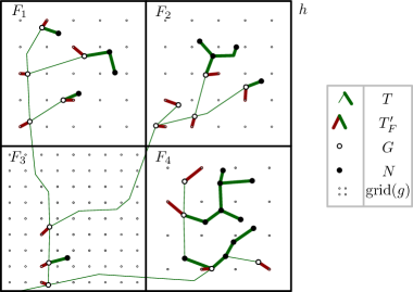
Figure 3: Construction of the forests $T^{\prime}_{F}$ in four faces in a plane $h$ of level $1$ in the quadtree. The green (thin and thick) edges are a schematic picture of $T$ (note that the actual edges consist only of axis-parallel segments), and the thick (red and green) edges indicate the forests $T^{\prime}_{F}$.

Construction of $T^{\prime}_{F}$.

Let $G$ be the set of (intuitively distant) vertices $x\in X\cap F$ such that $p(x)\notin F$, or the length of the line segment from $x$ to $p(x)$ is strictly greater than $L/(2^{i}r)$. We will now connect the vertices from $G$ to the nearest points on a grid with granularity $g$. Specifically, let $q$ be a positive integer such that $(q-1)^{d-1}<r^{2d-2}/|G|\leqslant q^{d-1}$, and let $g=q^{d-1}$ (since $r\geqslant 4$ such $q$ exists). Thus

$$\frac{r^{2d-2}}{|G|}\leqslant g<\frac{(2r)^{2d-2}}{|G|},$$ (6)

where the second inequality follows, since we assumed $r\geqslant 4$ and $|G|\leqslant m\leqslant(2r)^{d-1}$. Let $T_{F}:=T\cap F$ be the tree $T$ restricted to the cell $F$. We change $T_{F}$ to get a forest $T^{\prime}_{F}$ as follows. For each $z\in G$, remove the edge from $z$ to its parent in $T_{F}$ (if such an edge exists), and subsequently connect such a $z$ to the nearest point in $\mathrm{grid}(F,g)$. See Figure 3 for a schematic illustration of the construction for $d=3$.

Patching along $T^{\prime}_{F}$.

Next, we change the salesman path by applying Lemma 2.1 for all the connected components of $T^{\prime}_{F}$ in order to restrict the tour to cross the hyperplane $h$ only at $|G|$ points from $\mathrm{grid}(F,g)$. Additionally, if there is a point $p\in h$ and the path $\pi^{\prime}$ crosses $h$ more than twice at $p$, we apply Lemma 2.1 with $X=T=\{p\}$ and reduce the number of crossings at $p$ to at most two without increasing the length of $\pi^{\prime}$. This finishes the description of the construction of $\pi^{\prime}$ promised by the theorem.

$\pi^{\prime}$ crosses $h$ as required.

To see that the obtained path $\pi^{\prime}$ is $r$-simple, note that if $\pi$ crosses a facet $F$ of some cell in more than $1$ point then we alter it to make it cross at most $|G|$ times at points from $\mathrm{grid}(F,g)$. Since $g<(2r)^{2d-2}/|G|$, it follows that $\pi^{\prime}$ is $2r$-simple. By exchanging $r$ with $r/2$ in the whole proof, we therefore get an $r$-simple tour.

4.3 Analysis of the expected length of $\pi^{\prime}$

Let $\mathrm{cost}(h)$ denote the increase of the salesman path during the iteration corresponding to the hyperplane $h$. Our main effort will lie in proving that $\mathbb{E}\left[\mathrm{cost}(h)\right]\leqslant\mathcal{O}(\frac{d\sqrt{d}}{r}\cdot|I(\pi,h)|)=\mathcal{O}(\frac{d\sqrt{d}}{r}\cdot|X|)$. This would be sufficient to prove the theorem since it allows us to conclude that

$$\sum_{h\text{:grid hyperplane}}\mathbb{E}\left[\mathrm{cost}(h)\right]\leqslant\sum_{h\text{:grid hyperplane}}\mathcal{O}\left(d\sqrt{d}\cdot\frac{|I(\pi,h)|}{r}\right)=\mathcal{O}(d^{2}\cdot\mathrm{wt}(\pi)/r),$$ (7)

where the second inequality is by Lemma 2.2.

Setting up amortized patching costs.

For a point $x\in X$, let $\mathrm{pro}(x)$ be the proximity of $x$, which is defined as the length of the path from $x$ to its parent $p(x)$ in $T$ (the proximity of the root $r$ of $T$ is defined as $\infty$ for convenience). With each $x\in X$ we associate the following coefficients $\alpha_{i}(x)$ that represent the amortized expected patching cost due to $x$ if the level of $h$ is $i$:

$$\alpha_{i}(x)=\begin{cases}\displaystyle\mathrm{pro}(x)\cdot 2^{i}/L,&\textbf{if }\mathrm{pro}(x)\leqslant L/(2^{i}r),\\[7.5pt] \displaystyle\frac{d\sqrt{d}L}{\mathrm{pro}(x)\cdot 2^{i}r^{2}},&\textbf{if }L/(2^{i}r)<\mathrm{pro}(x)\leqslant L/2^{i},\\[12.50002pt] \displaystyle 0,&\textbf{if }L/2^{i}<\mathrm{pro}(x).\end{cases}$$

We will first show that the expected cost of patching from Lemma 2.1 for a fixed cell $F$ whose hyperplane has level $i$ is at most $\mathcal{O}(L/2^{i}\cdot\sum_{x\in F\cap X}\alpha_{i}(x))$. If $|F\cap X|\leqslant 1$, then this is true since Lemma 2.1 is not applied or applied only on a single point. For the other case it remains to analyze $\mathbb{E}\left[\mathrm{wt}(T^{\prime}_{F})\right]$, which we do next.

The expected weight of $T^{\prime}_{F}$.

Now we use the special properties of $T$ guaranteed by Lemma 4.1 to show the following.

Lemma 4.3.

It holds that:

$$\mathbb{E}[\mathrm{wt}(T^{\prime}_{F})]=\mathcal{O}\left(\frac{L}{2^{i}}\cdot\sum_{x\in F\cap X}\alpha_{i}(x)\right).$$

Proof.

Let $\rho_{F}$ be the root of $T_{F}$. Consider the following subset of $F\cap X$:

$$N :=\left\{x\in F\cap X:\mathrm{pro}(x)\leqslant\frac{L}{2^{i}r}\right\}\setminus\{\rho_{F}\}.$$

Therefore $N$ is a set of (near) vertices with small proximity. As $G$ consists of vertices with large proximity (i.e., it consists of $\rho_{F}$ and all vertices in $z\in X\cap F$ that satisfy $\mathrm{pro}(z)>L/(2^{i}r)$) we have that $X\cap F=N\cup G$.

Consider first the case $|G|=1$ (so $G=\{\rho_{F}\}$): Then

$$\mathrm{wt}(T^{\prime}_{F})=\mathrm{wt}(T_{F})=\sum_{x\in N}\mathrm{pro}(x)=\frac{L}{2^{i}}\sum_{x\in N}\alpha_{i}(x),$$

and the lemma follows. Thus, we may assume from now on that $|G|>1$. We bound $\mathrm{wt}(T^{\prime}_{F})$ from above by upper bounding the weight of the edge from $x$ to the parent of $x$ in $T^{\prime}_{F}$ in different ways depending on whether $x\in N$ or $x\in G$. If $x\in G$, then $x$ is connected in $T^{\prime}_{F}$ to the nearest point from $\mathrm{grid}(F,g)$, and the length of this connection is at most

$$\frac{L\sqrt{d-1}}{2^{i}g^{1/(d-1)}}<\frac{\sqrt{d}L}{2^{i}r^{2}}|G|^{1/(d-1)}$$ (8)

by the first inequality in (6). Let $T^{G}_{F}$ be the subtree of $T_{F}$ that connects $G$. By using Property (b) from Lemma 4.1 of $T$ with set $Q:=G$ and cell $F$, we have that $\mathrm{wt}(T^{G}_{F})<\frac{dL}{2^{i}}|G|^{1-1/(d-1)}$. Let $G^{\prime}:=G\setminus\{\rho_{F}\}$. By the $1$-lightness of $T$, for every $z\in G^{\prime}$ the edge from $z$ to the parent $p(z)$ of $z$ in $T_{F}$ is also present in $T^{G}_{F}$, and thus we have that $\sum_{z\in G^{\prime}}\mathrm{pro}(z)\leqslant\mathrm{wt}(T^{G}_{F})<\frac{dL}{2^{i}}|G|^{1-1/(d-1)}$. By Cauchy-Schwartz we therefore have that

$$|G^{\prime}|^{2}\leqslant\left(\sum_{z\in G^{\prime}}\mathrm{pro}(z)\right)\cdot\left(\sum_{z\in G^{\prime}}\frac{1}{\mathrm{pro}(z)}\right)<\frac{dL}{2^{i}}|G|^{1-\frac{1}{d-1}}\cdot\left(\sum_{z\in G^{\prime}}\frac{1}{\mathrm{pro}(z)}\right).$$

Because $|G^{\prime}|\geqslant 1$, we have that $|G|^{2}=(|G^{\prime}|-1)^{2}\leqslant 4|G^{\prime}|^{2}$ and we conclude that

$$|G|^{d/(d-1)}<4\frac{dL}{2^{i}}\sum_{z\in G}\frac{1}{\mathrm{pro}(z)}.$$ (9)

Now we bound the weight of the tree $T^{\prime}_{F}$ as follows:

$$\mathrm{wt}(T^{\prime}_{F}) <\sum_{y\in N}\mathrm{pro}(y)+\sum_{z\in G}\frac{\sqrt{d}L}{2^{i}r^{2}}\cdot|G|^{1/(d-1)}$$ (by (8))

$$=\sum_{y\in N}\mathrm{pro}(y)+\frac{\sqrt{d}L}{2^{i}r^{2}}\cdot|G|^{\frac{d}{d-1}}$$

$$<\sum_{y\in N}\mathrm{pro}(y)+4d\sqrt{d}\left(\frac{L}{2^{i}r}\right)^{2}\sum_{z\in G}\frac{1}{\mathrm{pro}(z)}$$ (by (9))

$$=\frac{L}{2^{i}}\cdot\mathcal{O}\left(\left(\sum_{y\in N}\frac{2^{i}}{L}\cdot\mathrm{pro}(y)\right)+\left(\sum_{z\in G}\frac{d\sqrt{d}}{r^{2}}\frac{L}{2^{i}}\frac{1}{\mathrm{pro}(z)}\right)\right)$$

$$=\mathcal{O}\left(\frac{L}{2^{i}}\sum_{x\in X\cap F}\alpha_{i}(x)\right).\qed$$

Wrapping up the expected patching cost analysis.

Recall that by Lemma 2.3, the hyperplane $h$ gets level $i$ with probability $2^{i-1}/L$. Thus we have

$$\mathbb{E}[\mathrm{cost}(h)]=\sum_{i=0}^{\log L}\frac{2^{i-1}}{L}\sum_{\begin{subarray}{c}F\text{ is facet of $C$ in }h,\\ \text{level of }C\text{ and }h\text{ is }i\end{subarray}}\mathbb{E}\left[\mathrm{wt}(T^{\prime}_{F})\right]=\mathcal{O}\left(\sum_{x\in X}\sum_{i=0}^{\log L}\alpha_{i}(x)\right).$$ (10)

On the other hand, for a fixed $x\in X$ we have that

$$\sum_{i=0}^{\log L}\alpha_{i}(x)=\sum_{i=0}^{\theta_{1}}\alpha_{i}(x)+\sum_{i=\theta_{1}+1}^{\theta_{2}}\alpha_{i}(x)\leqslant\frac{2}{r}+\frac{2d\sqrt{d}}{r}<\frac{3d\sqrt{d}}{r},$$ (11)

where we set $\theta_{1}:=\log(\frac{L}{\mathrm{pro}(x)\cdot r})$ and $\theta_{2}:=\log(\frac{L}{\mathrm{pro}(x)})$, and used the bound on a sum of geometric series twice. Combining (10) and (11) implies $\mathbb{E}[\mathrm{cost}(h)]=\mathcal{O}(\frac{d\sqrt{d}|X|}{r})=\mathcal{O}(\frac{d\sqrt{d}|I(\pi,h)|}{r})$, and thus the theorem follows from (7).

5 Approximate TSP in $\mathbb{R}^{d}$

In this section we prove Theorem 1.1. The first few steps of the algorithm are the same as in Arora’s algorithm [1], as outlined in Section 2.

In Step 1, we perturb points and assume that $P\subseteq\{0,\ldots,L\}^{d}$ for some integer $L=\mathcal{O}(n\sqrt{d}/\varepsilon)$ that is a power of $2$. Then in Step 2 we pick a random shift $\mathbf{a}\in_{R}\{0,\ldots,L\}^{d}$ and construct a compressed quadtree.

In Step 3 we use the following result by Rao and Smith [50] (the result can also be obtained by applying the procedure PATCH from [47] to the graph obtained from [47, Lemma 19.3.2]).

Lemma 5.1.

Given points set $P\subseteq\mathbb{R}^{d}$ let $\pi$ be the optimum TSP tour of $P$. Then there is a $\mathrm{poly}(1/\varepsilon)n+T_{\mathrm{spanner}}(n,\varepsilon)$ time ⁶ algorithm that given $P$ and the random offset $\mathbf{a}$ of the dissection, computes a set of line segments $S$ such that

1. if $\pi^{S}$ is the shortest tour of $P$ among the tours that use only edges from $S$, then $\mathbb{E}_{\mathbf{a}}[\mathrm{wt}(\pi^{S})-\mathrm{wt}(\pi)]=\mathcal{O}(\varepsilon\cdot\mathrm{wt}(\pi))$.

2. $S$ is $1/\varepsilon^{\mathcal{O}(d)}$-light with respect to $D(\mathbf{a})$

The algorithm also stores for each face $F$ of each cell $C$ of $\mathrm{CQT}(P,\mathbf{a})$ all crossings of $S$ and $F$. $T_{\mathrm{spanner}}(n,\varepsilon)$ is the time needed to compute a light $(1+\varepsilon)$ spanner of $n$ points.

Let $\pi$ be the optimum TSP tour on the perturbed point set $P$. Lemma 5.1 gives us the set $S$ with the property that (i) there exist $\pi^{S}$ that uses only edges from $S$, and (ii) in expectation the extra weight of $\pi^{S}$ is only $\mathcal{O}(\varepsilon\cdot\mathrm{wt}(\pi))$, and (iii) $\pi^{S}$ crosses every cell of the quadtree at most $1/\varepsilon^{\mathcal{O}(d)}$ times. This summarizes all the steps from previous work that we will use in the algorithm.

We apply Theorem 3.3 to $\pi^{S}$, which guarantees the existence of an $r$-simple tour that is a good approximation in expectation, and it has the property that quadtree faces crossed only once will be crossed at the same place as in $\pi^{S}$. Now, in Step 4 (that we describe in full detail in the next section) we find the optimal $r$-simple tour with this property. Similarly to Arora (and to the description in Section 2) we use a dynamic programming algorithm for this. There are however two crucial changes. First, we cannot bound the number of matchings in $d>2$ the same way as we did for $d=2$, since we used the non-crossing property for this. For this reason, we will combine the dynamic programming with the the rank-based approach [10]. In order to get the more efficient $\mathcal{O}(n\log n)$ running time dependence on $n$, we will use a portal set consisting of all crossings with the cell boundary and the set of line segments $S$ from Lemma 5.1 when the tour has only one crossing point in a given facet.

Finally, in Step 5 we will trim the edges of the obtained salesman path (just as [1]) to make it a proper solution to the TSP problem. This can only decrease the weight of the solution and is straightforward. In Section 5.1 we explain Step 4 of our procedure. In Section 5.2 we analyze the total running time and the approximation ratio.

5.1 Dynamic Programming

We use a dynamic programming algorithm to find an $\mathcal{O}(1/\varepsilon)$-simple salesman tour with respect to the shifted quadtree (in a similar fashion to Arora [1]). With high probability, this salesman tour has weight $(1+\varepsilon)\cdot\mathrm{wt}(\text{OPT})$. The running time of this step is $2^{\mathcal{O}(1/\varepsilon^{d-1})}n$.

The dynamic programming algorithm works as follows. It iterates through the compressed quadtree in a bottom-up fashion: We start with the smallest quadtree cells on the lowest level and based on them, compute the minimum solution one level higher. In subproblems that correspond to non-compressed internal vertices of the quadtree, we are no longer searching for a shortest tour that connects all points inside, but rather for a collection of paths that connect neighboring cells of a quadtree in the prescribed manner. For a given quadtree cell $C$ let $\partial C$ denote its boundary. The Structural Theorem (Theorem 3.3) guarantees the existence of some set of portals $B\subseteq\partial C$ that will be traversed by the tour. In our subproblem we fix such a set $B$ and we are also given a perfect matching $M$ on $B$. We say that a collection $\mathcal{P}:=\{\pi_{1},\ldots,\pi_{|B|/2}\}$ of paths realizes $M$ on $B$ if for each $(p,q)\in M$ there is a path $\pi_{i}\in\mathcal{P}$ with $p$ and $q$ as endpoints.

For each facet $F$ there is a unique maximum facet $\mathrm{ex}(F)$ that is the boundary of a cell in the compressed quadtree that contains $F$. Note that when considering the cell $C$ and one of its facets $F$, we will place the portals according to the grids of $\mathrm{ex}(F)$, or potentially at some point in $F\cap S$. We say that $B$ is fine with respect to $S$ if for all facets $F$ of $C$ we have that either (i) $B\cap F=\{p\}$ and $p\in S\cap F$, or (ii) $B\subset\mathrm{grid}(\mathrm{ex}(F),r^{2d-2}/m_{F})$ where $|B\cap F|\leqslant m_{F}\leqslant r^{d-1}$. Note that the first option is needed because in Definition 3.2 we often need a perfect precision on faces that are crossed exactly once.

The subproblems are defined as follows (cf., $r$-multipath problem in Arora [1]).

$r$-Multipath Problem Input: A nonempty cell $C$ in the shifted quadtree, a portal set $B\subseteq\partial C$ that is fine with $S$, and a perfect matching $M$ on $B$. Task: Find an $r$-simple path collection $\mathcal{P}_{B,M}$ of minimum total length that satisfies the following properties. • The paths in $\mathcal{P}_{B,M}$ visit all input points inside $C$. • $\mathcal{P}_{B,M}$ crosses $\partial C$ only through portals from $B$. • $\mathcal{P}_{B,M}$ realizes the matching $M$ on $B$.

Arora [1] defined the multipath problem in a similar way. The main difference is that he considers all $B\subseteq\bigcup_{F}\mathrm{grid}(\mathrm{ex}(F),r^{2d-2})$, while our structural Lemma enables us to select $B\subseteq\bigcup_{F}\mathrm{grid}(\mathrm{ex}(F),r^{2d-2}/m)$ of size $m$ (apart from the special case with $1$ crossing on the facet). Arora [1] showed how to use dynamic programming to solve the $r$-Multipath problem in time $\mathcal{O}(n\cdot m^{\mathcal{O}(r)})$ (for $d=2$) which is already too expensive in our case for $m,r=\mathcal{O}(1/\varepsilon)$. Here and below, the union is taken over all facets $F$ of the given cell $C$.

Before we explain our approach in detail, let us explain the natural dynamic programming algorithm for $d=2$ and why it is not fast enough for $d>2$. The dynamic programming builds a lookup table that contains the costs of all instances of the multipath problem that arise in the quadtree (exactly the same as in Arora [1]). When the table is built, it is enough to output the entry that corresponds to the root of the quadtree. The number of non-empty cells in the compressed quadtree is $\mathcal{O}(n)$. For each facet $F$ of the cell $C$, we guess an integer $m_{F}\leqslant 1/\varepsilon^{d-1}$ that is the number of times the $\mathcal{O}(1/\varepsilon^{d-1})$-simple salesman tour crosses it. Then, we select a set $|B|=m$ by selecting a set of size $m$ from $\bigcup_{F}\mathrm{grid}(\mathrm{ex}(F),r^{2d-2}/m_{F})$, where $\sum_{F}m_{F}=m$. There are at most $\prod_{F}\binom{r^{2d-2}/m_{F}}{m_{F}}\leqslant 2^{2d\cdot\mathcal{O}(r^{d-1})}\leqslant 2^{\mathcal{O}(r^{d-1})}$ possible choices for the portal set $B$ by Claim 3.4, since the number of facets $F$ of $C$ is at most $2d$. Unfortunately, the number of perfect matchings on $m$ points is $2^{\mathcal{O}(m\log{m})}$. This would lead to a running time of $2^{\mathcal{O}(1/\varepsilon^{d-1}\log(1/\varepsilon))}$, which has an extra $\log(1/\varepsilon)$ factor in the exponent compared to our goal. Recall that in $d=2$ we could use that an optimal TSP tour is crossing-free and it was efficient to look for “crossing-free matchings” (and their number is at most $2^{\mathcal{O}(m)}$). To reduce the number of possible matchings in $d>2$ we will use the rank-based approach.

Rank-based approach

Now we describe how the rank-based approach [10, 15] can be applied in this setting. We will heavily build upon the methodology and terminology from [10], and describe the basics here for the unfamiliar reader. We follow the notation from [19].

Let $C$ be the cell of the quadtree and let $B\subseteq\partial C$ be the set of portals on its boundary with $|B|=m$ (note that $m$ is even). We define the weight of a perfect matching $M$ of $B$ to be the total length of the solution to the multipath problem on $(C,B,M)$, and denote it by $\mathrm{wt}(M)$. A weighted matching on $B$ is then a pair $(M,\mathrm{wt}(M))$ for some perfect matching $M$. Let $\mathcal{M}(B)$ denote the set of all weighted matchings on $B$.

We say that two perfect matchings $M_{1},M_{2}$ fit if their union is a Hamiltonian Cycle on $B$. For some set $\mathcal{R}[B]\subseteq\mathcal{M}(B)$ of weighted matchings and a fixed perfect matching $M$ we define

$$\text{opt}(M,\mathcal{R}[B]):=\min\left\{\text{weight}(M^{\prime})\;:\;(M^{\prime},\text{weight}(M^{\prime}))\in\mathcal{R}[B]\text{ and }M^{\prime}\text{ fits }M\right\}$$

Finally, we say that the set $\mathcal{R}[B]\subseteq\mathcal{M}(B)$ is representative if for any matching $M$, we have $\text{opt}(M,\mathcal{R}[B])=\text{opt}(M,\mathcal{M}(B))$. The crucial theorem behind the rank-based approach is the following result.

Lemma 5.2 (Theorem 3.7 in [10]).

There exists a set $\mathcal{R}^{\star}[B]$ of $2^{|B|/2-1}$ weighted matchings that is representative of $\mathcal{M}(B)$. There is an algorithm $\mathtt{Reduce}$ that given some representative set $\mathcal{R}[B]$ of $\mathcal{M}(B)$ computes a set $\mathcal{R}^{\star}$ in $|\mathcal{R}^{\star}[B]|\cdot 2^{\mathcal{O}(|B|)}$ time.

In the following, $\mathcal{R}:=\bigcup_{B}\{\mathcal{R}[B]\}$ for $B\subseteq\partial C$ that are with $S$. For convenience, we say that the family $\mathcal{R}$ is representative if every $\mathcal{R}[B]\in\mathcal{R}$ is representative.

Now, we are ready to describe the solution to the $r$-Multipath problem (see Algorithm 2 for global pseudocode). The algorithm is given a quadtree cell $C$ and a set of line segments $S$. The task is to output the union of sets $\mathcal{R}^{\star}[B]$ for every $B\subseteq\partial{C}$, where $B$ has size $m$ and it is fine with $S$, and $\mathcal{R}^{\star}[B]$ is representative of $\mathcal{M}(B)$. We start the description of the algorithm with a case distinction based on which type the given cell of the quad tree has. In the base case we consider a cell that has one or zero points. Next we consider another special case, i.e., the compressed case, when the given cell has only one child in the compressed quadtree. After that, we show how to combine $2^{d}$ children in the paragraph non-compressed non-leaf case.

Base case

We start with the base case, where the cell $C$ is a leaf of the quadtree and contains at most one input point. Consider all possible sets $B$ that are fine with $S$. This gives an instance of at most $|B|+1$ points and we can use an exact algorithm to get a set $\mathcal{R}^{\star}[B]$ in time $2^{\mathcal{O}(|B|)}$. We can achieve that with a standard dynamic programming procedure: Let us fix $B$ and let $p$ be the only input point inside $C$ (if it exists). For every $X\subseteq B$ we will compute a table $\mathtt{BC}[X]$ that represents $\mathcal{M}(X)$ for every $X\subseteq B$. Initially $\mathtt{BC}[\emptyset]=\{(\emptyset,0)\}$ and if $p$ exists, then for every $a,b\in B$ let $\mathtt{BC}[a,b]:=\{\{(a,b)\},\mathrm{dist}(a,p)+\mathrm{dist}(p,b)\}$, which means that $p$ is connected to the portals $a,b\in B$. Next, we compute $\mathtt{BC}[X]$ for every $X\subseteq B$ with the following dynamic programming formula.

$$\mathtt{BC}[X]:=\mathtt{reduce}\left(\bigcup_{\begin{subarray}{c}u,v\in X\\ u\neq v\end{subarray}}\left\{\big{(}M\cup\{(u,v)\},\mathrm{wt}(M)+\mathrm{dist}(u,v)\big{)}\;\Big{|}\;(M,\mathrm{wt}(M))\in\mathtt{BC}[X\setminus\{u,v\}]\right\}\right)$$

For a fixed $B$ this algorithm runs in $\mathcal{O}(|\mathcal{R}^{\star}[B]|\cdot 2^{\mathcal{O}(|B|)})$ time and correctly computes $\mathtt{BC}[B]=\mathcal{R}^{\star}[B]$ (cf., [10, Theorem 3.8] for details of an analogous dynamic programming subroutine).

Compressed case

In this case we are given a large cell $C_{\mathrm{out}}$ and its only child $C_{\mathrm{in}}$. From the dynamic programming algorithm we know the solution to $C_{\mathrm{in}}$ for all relevant $B_{\mathrm{in}}\subseteq\partial C_{\mathrm{in}}$ and the task is to connect these portals to the portals $B_{\mathrm{out}}\subseteq C_{\mathrm{out}}$. We do dynamic programming similar to the one seen in the base case. We say that a pair $B_{\mathrm{in}},B_{\mathrm{out}}$ where $B_{\mathrm{out}}\subset\partial C_{\mathrm{out}}$ and $B_{\mathrm{in}}\subset\partial C_{\mathrm{in}}$ are fine with $S$ if they are individually fine with $S$, and if $\partial C_{\mathrm{out}}\cap\partial C_{\mathrm{in}}\neq\emptyset$ then $B_{\mathrm{out}}\supset B_{\mathrm{in}}\cap\partial C_{\mathrm{out}}$. For each fixed pair $B_{\mathrm{out}},B_{\mathrm{in}}$ that are fine with $S$, we compute a table $\mathtt{DBC}[X]$ (mnemonic fordummy base case) that represents $\mathcal{M}(X)$ (where the paths need not cover any input points) for every multiset $X\subseteq B_{\mathrm{out}}\uplus B_{\mathrm{in}}$. Note that the cell $C_{\mathrm{out}}$ can be regarded as the disjoint union of $C_{\mathrm{in}}$ and a dummy leaf cell that has region $C_{\mathrm{out}}\setminus C_{\mathrm{in}}$. Initially, we set $\mathtt{DBC}[\emptyset]=\{(\emptyset,0)\}$. We can then compute the values for the dummy base cases $\mathtt{DBC}$ with the same formula as for the base case.

$$\mathtt{DBC}[X]:=\mathtt{reduce}\left(\bigcup_{\begin{subarray}{c}u,v\in X\\ u\neq v\end{subarray}}\left\{\big{(}M\cup\{(u,v)\},\mathrm{wt}(M)+\mathrm{dist}(u,v)\big{)}\;\Big{|}\;(M,\mathrm{wt}(M))\in\mathtt{DBC}[X\setminus\{u,v\}]\right\}\right)$$

Let $\mathcal{R}^{\star}$ be the table of these sets for all $B_{\mathrm{out}},B_{\mathrm{in}}$ that are fine with $S$, i.e., $\mathcal{R}^{\star}[X]=\mathtt{DBC}(X)$ for all $X\subseteq B_{\mathrm{out}}\cup B_{\mathrm{in}}$. In order to get representative sets $\mathcal{R}[B_{\mathrm{out}}]$ of $\mathcal{M}(B_{\mathrm{out}})$ for every $B_{\mathrm{out}}\subset\partial C_{\mathrm{out}}$ that is fine with $S$, we can combine the representative set $\mathcal{R}_{\mathrm{in}}^{\star}$ of $C_{\mathrm{in}}$ and $\mathcal{R}^{\star}$ (see Algorithm 1).

Algorithm : $\mathtt{CompressedCase}(C_{\mathrm{in}},C_{\mathrm{out}},\mathcal{R}^{\star}_{\mathrm{in}})$. $C_{\mathrm{out}}$ is a compressed cell and $C_{\mathrm{in}}$ its child

1 Let $\mathcal{R}^{\star}_{\mathrm{dummy}}[X]\leftarrow\mathtt{DST}(X)$ for every relevant $X\subseteq B_{\mathrm{in}}\ \cup B_{\mathrm{out}}$

2 foreach $M_{\mathrm{in}}\in\mathcal{R}^{\star}_{\mathrm{in}},M_{\mathrm{dummy}}\in\mathcal{R}^{\star}_{\mathrm{dummy}}$ do

3       if $M_{\mathrm{in}}$, $M_{\mathrm{dummy}}$ are compatible then

4             Let $M_{\mathrm{out}}\leftarrow\mathtt{Join}(M_{\mathrm{in}},M_{\mathrm{dummy}})$

5             Let $B_{\mathrm{out}}\leftarrow$ ground set of $M_{\mathrm{out}}$

6              // Note that $B_{\mathrm{out}}\subset\partial C_{\mathrm{out}}$

7             if $B_{\mathrm{out}}$ is fine with respect to $S$ then

8                   Insert $\big{(}M_{\mathrm{out}},\,\mathrm{wt}(M_{\mathrm{in}})+\mathrm{wt}(M_{\mathrm{dummy}})\big{)}$ into $\mathcal{R}[B_{\mathrm{out}}]$

9foreach $B_{\mathrm{out}}\subset\partial C_{\mathrm{out}}$ that is fine with $S$ do

10       $\mathcal{R}[B_{\mathrm{out}}]\leftarrow\mathtt{reduce}(\mathcal{R}[B_{\mathrm{out}}])$

return $\mathcal{R}$

Algorithm 1 Pseudocode for compressed cells

The algorithm and the analysis is similar to the dynamic programming algorithm below (hence we skip the description and formal analysis). For a fixed $B_{\mathrm{out}}$ and $B_{\mathrm{in}}$ this algorithm runs in $\mathcal{O}(|\mathcal{R}^{\star}[B_{\mathrm{out}}]|\cdot|\mathcal{R}^{\star}[B_{\mathrm{in}}]|\cdot 2^{\mathcal{O}(|B_{\mathrm{out}}|+|B_{\mathrm{in}}|)})$ time and correctly computes the distances and matchings for every that are $B_{\mathrm{out}}\subseteq\partial C_{\mathrm{out}}$, $B_{\mathrm{in}}\subseteq\partial C_{\mathrm{in}}$ that are fine with $S$.

Non-compressed non-leaf case

For non-compressed non-leaf cells $C$ we combine the solutions of cells of one level lower. Let $C_{1},\ldots,C_{2^{d}}$ be the children of $C$ in the compressed quadtree. Also, let $\mathcal{R}_{i}$ be the solution to the $r$-Multipath problem in cell $C_{i}$ that we get recursively. Next we iterate over every $M_{1}\in\mathcal{R}_{1},\ldots,M_{2^{d}}\in\mathcal{R}_{2^{d}}$ and check if matchings $M_{1},\ldots,M_{2^{d}}$ are compatible. By this, we mean that (i) for every neighboring cell $S_{i},S_{j}$ the endpoints of matchings on their shared facet are the same and (ii) combining $M_{1},\ldots,M_{2^{d}}$ results in a set of paths with endpoints in $\partial C$.

Algorithm : $\mathtt{MultipathProblem}(C,S,r)$

Output : Family $\mathcal{R}$, which is the union of sets $\mathcal{R}[B]$ of weighted matchings that represent $\mathcal{M}(B)$ for each $B$ that is fine with $S$

1 if $|C\cap P|\leqslant 1$ then $\mathcal{R}\leftarrow$ base case with one or no points

2 else if $C$ is compressed then

3       Let $C_{+}$ be the only child of $C$ and $\mathcal{R}_{+}$ solution on $C_{+}$

4       $\mathcal{R}\leftarrow\mathtt{CompressedCase}(C,C_{+},\mathcal{R}_{+})$

5else

6       Let $C_{1},\ldots,C_{2^{d}}$ be the children of $C$

7       Let $\mathcal{R}_{i}\leftarrow\mathtt{MultipathProblem}(C_{i},S,r)$

8       foreach $M_{1}\in\mathcal{R}_{1},\ldots,M_{2^{d}}\in\mathcal{R}_{2^{d}}$ do

9             if $M_{1},M_{2}$…and $M_{2^{d}}$ are compatible then

10                   Let $M\leftarrow\mathtt{Join}(M_{1},\ldots,M_{2^{d}})$, let $B\leftarrow$ ground set of $M$

11                   if  $B$ is fine with respect to $S$ then

12                         Insert $\big{(}M,\,\mathrm{wt}(M_{1})+\ldots+\mathrm{wt}(M_{2^{d}})\big{)}$ into $\mathcal{R}$

13      foreach $B\subset\partial C$ that is fine with $S$ do

14             $\mathcal{R}[B]\leftarrow\mathtt{reduce}(\mathcal{R}[B])$

return $\mathcal{R}$

Algorithm 2 Pseudocode of the dynamic programming for the Multipath problem

Next, if the matchings $M_{1},\ldots,M_{2^{d}}$ are compatible, we join them (join can be thought of as $2^{d}-1$ joins of matchings defined in [10]). This operation will give us the matching obtained from $M_{1}\cup\ldots\cup M_{2^{d}}$ by contracting degree two edges if no cycle is created, and gives us matchings on the boundary (i.e., set $B$) and information about connection between these points (i.e., a matching $M$ on the set $B$).

If $B$ is fine with $S$, then we insert $M$ into $\mathcal{R}[B]$ with weight being the sum of the weights of matchings $M_{1},\ldots,M_{2^{d}}$. At the end we will use the operation reduce to decrease the sizes of all $\mathcal{R}[B]$ and still get a representative set of size $2^{\mathcal{O}(|B|)}$. The corresponding pseudo-code is given in Lines 2 to 2 of Algorithm 2.

Overall Algorithm

Lemma 5.3.

For a cell $C$ and a fixed $B$ that is fine with respect to $S$, the set $\mathcal{R}[B]$ computed in Algorithm 2 is representative of $\mathcal{M}(B)$.

Proof.

The proof is by induction on $|C\cap P|$. For $|C\cap P|\leqslant 1$ the lemma follows from the correctness of the base case. Next we assume that $|C\cap P|>1$ and has some children $C_{1},\ldots,C_{2^{d}}$ in the quadtree. Let us fix some $B\subseteq\partial C$ of size $m$ that is fine with respect to $S$, a matching $M$ on $B$ and an optimal solution, i.e., collection of $r$-simple paths $OPT(S,B,M,r)=\{\pi_{1},\ldots,\pi_{|B|/2}\}$ with distinct endpoints in $B$ that realize matching $M$. Because $OPT(S,B,M,r)$ is $r$-simple, there exists $B_{1}\subseteq\partial C_{1},\ldots,B_{2^{d}}\subseteq\partial C_{2^{d}}$ that are fine with respect to $S$ and matchings $M_{1},\ldots,M_{2^{d}}$ on $B_{1},\ldots,B_{2^{d}}$ such that $OPT(S,B,M,r)$ crosses boundaries between $C_{1},\ldots,C_{2^{d}}$ exactly in $B_{1},\ldots,B_{2^{d}}$ and the matchings $M_{1},\ldots,M_{2^{d}}$ are compatible and their join is $M$. Hence in Line 2, Algorithm 2 finds $B$ and the matching $M$. Next we will insert it with the weight $\mathrm{wt}(OPT(S,B,M,r))$ to the set $\mathcal{R}[B]$. Since the join operation preserves representation (see [10, Lemma 3.6]), the set $\mathcal{R}[B]$ is a representative set. Finally, by Lemma 5.2 we assert that the $\mathtt{reduce}$ algorithm also outputs a representative set. An analogous argument shows that the sets $\mathcal{R}[B]$ computed for compressed cells are also representative. ∎

Lemma 5.4.

Algorithm 2 runs in time $\mathcal{O}(n\cdot|\mathcal{R}|^{2^{\mathcal{O}(d)}}\cdot 2^{\mathcal{O}(|B|)})$, where $n$ is the number of points in $C$.

Proof.

In the algorithm, we use a compressed quadtree, therefore the number of cells to consider is $\mathcal{O}(n)$. Algorithm 2 in the base case runs in time $\sum_{B}|\mathcal{R}|2^{\mathcal{O}(|B|)}=|\mathcal{R}|^{\mathcal{O}(1)}2^{\mathcal{O}(|B|)}$. The for loop in Line 2 of Algorithm 2 has $|\mathcal{R}_{1}|\cdots|\mathcal{R}_{2^{d}}|=\mathcal{O}(|\mathcal{R}|)^{2^{d}}$ many iterations, and the analogous for loop in the compressed case has $|\mathcal{R}_{\mathrm{in}}|\cdot|\mathcal{R}^{\star}_{\mathrm{empty}}|2^{\mathcal{O}(|B|)}=2^{\mathcal{O}(|B|)}|\mathcal{R}|^{\mathcal{O}(1)}$ iterations. Checking whether matchings $M_{1},\ldots,M_{2^{d}}$ are compatible and joining them takes $\mathrm{poly}(r,2^{d})$ time. Moreover, checking whether $B$ is fine with respect to the set $S$ can be checked in $r^{\mathcal{O}(d)}$ time because Lemma 5.1 guarantees us that access to these points can be achieved through the lists. The for loop in Line 2 of Algorithm 2 has at most $|\mathcal{R}|$ many iterations. In each iteration we invoke $\mathtt{reduce}$ procedure that takes $|\mathcal{R}|\cdot 2^{\mathcal{O}(|B|)}$ time according to Lemma 5.2. Note that the running times in the compressed case can be bounded the same way. This yields the claimed running time. ∎

Claim 5.5.

$|\mathcal{R}|\cdot 2^{\mathcal{O}(|B|)}\leqslant 2^{\mathcal{O}(r^{d-1})}$

Proof.

First, note that $|B|\leqslant 2^{d}r^{d-1}$ by the bound in Definition 3.2. Next, we bound the number of possible sets $B$. We select sets $B\cap F$ of size $b_{F}$, where the points can be chosen from $\mathrm{grid}(\mathrm{ex}(F),r^{2d-2}/m_{F})$ where $|B\cap F|\leqslant m_{F}\leqslant r^{d-1}$ or (when some point crosses one of the $2^{d}$ facets exactly once) it can also be chosen from $S\cap F$.

Hence, there are at most

$$\binom{|S\cap\partial C|}{2^{d}}\cdot\prod_{F}\left(\sum_{m_{F}=1}^{(2r)^{d-1}}\sum_{b_{F}=1}^{m_{F}}\binom{r^{2d-2}/m_{F}}{b_{F}}\right)$$

possible choices for $B$. Recall, that there is at most $2^{\mathcal{O}(d)}$ possible facets $F$. Moreover, Lemma 5.1 guarantees that $S$ crosses each face at most $1/\varepsilon^{\mathcal{O}(d)}$ times, hence $|S\cap F|\leqslant 1/\varepsilon^{\mathcal{O}(d)}$ and $\binom{|S\cap\partial C|}{2^{d}}\leqslant r^{2^{\mathcal{O}(d)}}$. By Claim 3.4, $\binom{r^{2d-2}/m_{F}}{b_{F}}$ is bounded by $2^{\mathcal{O}(r^{d-1})}$. Therefore the number of possible choices for $B$ is at most

$$r^{2^{\mathcal{O}(d)}}\cdot\prod_{F}\left(\sum_{m_{F}=1}^{(2r)^{d-1}}\sum_{b_{F}=1}^{m_{F}}2^{\mathcal{O}(r^{d-1})}\right)=2^{\mathcal{O}(r^{d-1})}.$$

Next we bound $\mathcal{R}[B]$ for a fixed $B$. Note that in Algorithm 2, we always use subroutine $\mathtt{reduce}$ to reduce the size of $\mathcal{R}[B]$. Lemma 5.2 guarantees that this procedure outputs a set $\mathcal{R}^{\star}[B]$ of size at most $2^{|B|-1}$. Multiplying all these factors gives us the desired property. ∎

Combining all of the above observations gives us the following Corollary.

Corollary 5.6.

Suppose we are given a compressed quadtree $Q$ and a point set $P$ of cardinality $n$ and a set $S$ of segments that crosses each full facet of $Q$ in at most $r^{\mathcal{O}(d)}$ points. Let $\pi^{S}\subseteq S$ be the shortest salesman path of $P$ within $S$. Then in $n\cdot 2^{\mathcal{O}(r^{d-1})}$ time we can find the shortest $r$-simple salesman path $\pi^{\prime}$ that (i) visits all the points in $P$, and (ii) if $\pi^{S}$ crosses any facet of $Q$ exactly once, then $\pi^{\prime}$ crosses it at the same point.

5.2 Proof of Theorem 1.1

In this Section we analyze the running time and approximation ratio of Theorem 1.1. For the running time observe that Step 1, 2, 3 and 5 take $\mathrm{poly}(1/\varepsilon)\cdot n\log{n}$ time. In Step 4 we set $r$ to $\mathcal{O}(d^{2}/\varepsilon)$ and by Corollary 5.6 we get an extra $n\cdot 2^{\mathcal{O}(d^{2}/\varepsilon)^{d-1}}$ factor. Overall, this gives the claimed running time.

For the approximation ratio, assume that $\pi$ is the optimal solution. Note that Step 1 perturbs the solution by at most $\mathcal{O}(\varepsilon\cdot\mathrm{wt}(\pi))$. In Step 3, by the Lemma 5.1 we are guaranteed that there exists a tour $\pi^{S}$ of weight $\mathcal{O}(\varepsilon\cdot\mathrm{wt}(\pi))$ larger than $\pi$ (in expectation). Next in Step 4, Corollary 5.6 applied to the set $S$, guarantees that that we find a salesman path $\pi^{\prime}$ that satisfies the condition of Structural Theorem 3.3 for $\pi^{S}$. It means that $\mathbb{E}_{\mathbf{a}}[\mathrm{wt}(\pi^{\prime})-\mathrm{wt}(\pi^{S})]=\mathcal{O}(\varepsilon\cdot\mathrm{wt}(\pi))$ and $\mathrm{wt}(\pi^{\prime})=(1+\mathcal{O}(\varepsilon))\mathrm{wt}(\pi)$. Applying Step 5 on $\pi^{\prime}$ can only decrease the total weight of $\pi^{\prime}$. This concludes the proof of Theorem 1.1.

It is easy to see that the algorithm can be derandomized by trying all possibilities for $\mathbf{a}$.

5.3 Extension to Euclidean and Rectilinear Steiner Tree

In this subsection, we consider extensions to two variants of Steiner Tree: Euclidean Steiner Tree and Rectilinear Steiner Tree. As most techniques work the same way for these problems, we only sketch the differences between the algorithms.

Arora’s patching procedure and structure theorem both seamlessly extend to optimum trees both for the Euclidean and the rectilinear versions, and the same holds for our patching and structure theorem. It is therefore only the algorithm that needs adjusting.

The notion of spanners for the Steiner tree problems is more complicated (one requires so-called banyans). We summarize this notion at the end of this section. Similarly to how we used spanners for the algorithm for TSP, here we use “banyan” to determine a set $\tilde{S}$ of points. This will consists of $(1/\varepsilon)^{\mathcal{O}(d)}$ portals for each facet that we use in the case of single crossing. Consequently, we say that a portal set $B\subset\partial C$ is valid with respect to $\tilde{S}$ if for each facet $F$ of $C$ we have that either (i) $B\cap F=\{p\}$ and $p\in\tilde{S}\cap F$, or (ii) $B\subset\mathrm{grid}(\mathrm{ex}(F),r^{2d-2}/m_{F})$ where $|B\cap F|\leqslant m_{F}\leqslant r^{d-1}$.

Additionally, we need to track connectivity requirements with partitions instead of matchings. A partition $M$ of $B$ is realized by a forest if for any $b,b^{\prime}\in B$ we have that $b$ and $b^{\prime}$ are in the same tree of the forest if and only if they are in the same partition class of $M$. The problem we need to solve in cells is the following.

$r$-Simple Steiner Forest Problem Input: A nonempty cell $C$ in the shifted quadtree, a portal set $B\subseteq\partial C$ that is valid with $\tilde{S}$, and a partition $M$ on $B$ Task: Find an $r$-simple forest $\mathcal{P}_{B,M}$ of minimum total length that satisfies the following properties. • The forest $\mathcal{P}_{B,M}$ spans all input points inside $C$. • $\mathcal{P}_{B,M}$ crosses $\partial C$ only through portals from $B$. • $\mathcal{P}_{B,M}$ realizes the partition $M$ on $B$.

The rank-based approach [10, 15] was originally conceived with partitions in mind, and therefore we can still use representative sets and the reduce algorithm as before (although the upper bound on $\mathcal{R}^{\star}[B]$ of $2^{|B|/2-1}$ from Lemma 5.2 needs to be increased to $2^{|B|-1}$).

The main difference between TSP and Steiner Tree is the handling of leaf and dummy leaf cells (i.e., the base case and the dynamic programming in the compressed case).

Leaves and dummy leaves for Rectilinear Steiner Tree.

Consider now a point set $Q\subset\mathbb{R}^{d}$. The Hanan-grid of $Q$ is the set of points that can be defined as the intersection of $d$ distinct axis-parallel hyperplanes incident to $d$ (not necessarily distinct) points of $Q$. By Hanan’s and Snyder’s results [31, 51], the optimum rectilinear Steiner tree for a given point set $Q$ lies in the Hanan-grid of $Q$. In particular, in a leaf cell our task is to find a representative set for a fixed set of $k=\mathcal{O}(1/\varepsilon)^{d-1}$ terminals (which includes the input point in case of a non-empty leaf cell.) Note that for each fixed $B$ this task can be done in the graph $G$ defined by the Hanan-grid of $B\cup(C\cap P)$, where the edge weights correspond to the $\ell_{1}$ distance. The graph $G$ has $\mathrm{poly}(1/\varepsilon)$ vertices and edges. Let $H$ be the set of vertices in the Hanan-grid of $B$, i.e., the set of possible Steiner Points for the terminal set $B$, where $B$ is the set of portals on the boundary of the cell.

To solve the base case efficiently, we will use a dynamic programming subroutine inspired by the classical Dreyfus-Wagner algorithm [23]. Let $\mathtt{ST}[D,v]$ be the minimum possible weight of a Steiner Tree for $D\cup\{v\}$, for all $D\subseteq B$ and $v\in H$. In the base case $\mathtt{ST}[\{b\},v]=\lVert b-v\rVert_{1}$. We can compute it efficiently with the following dynamic programming formula:

$$\mathtt{ST}[D,v]:=\min_{\begin{subarray}{c}u\in H\\ \emptyset\neq D^{\prime}\subset D\end{subarray}}\Big{\{}\mathtt{ST}[D^{\prime},u]+\mathtt{ST}[D\setminus D^{\prime},u]+\lVert u-v\rVert_{1}\Big{\}}.$$

This algorithm correctly computes a minimum weight Steiner Tree that connects $D\subseteq B$ and the running time of this algorithm is $2^{\mathcal{O}(|B|)}\cdot\mathrm{poly}(1/\varepsilon)$ (see [23]). Finally, let $\mathtt{ST}[X]:=\min_{v}\mathtt{ST}[X,v]$.

Next, we take care of all partitions of $B$. This involves a similar dynamic programming as in the base case of TSP. Let $\mathtt{SF}(X)$ be the set $\mathcal{R}^{\star}[X]$ that represents every partition of $X\subseteq B$. Namely, for every Steiner forest $F$ with connected components $B_{1},\ldots,B_{k}$, such that $B_{1}\uplus\ldots\uplus B_{k}=X$ there exists $M\in\mathcal{R}^{\star}[X]$, such that the union of $F$ and a forest $F_{M}$ whose connected components correspond to $M$ gives a tree that spans $X$. At the beginning, we set $\mathtt{SF}[\emptyset]=\{\emptyset,0\}$. Next, we use the following dynamic programming to compute $\mathtt{SF}[X]$ for all $X\subset B$:

$$\mathtt{SF}[X]:=\mathtt{reduce}\left(\bigcup_{Y\subseteq X}\Big{\{}(M\cup\{Y\},\mathrm{wt}(M)+\mathtt{ST}[Y])\;\Big{|}\;(M,\mathrm{wt}(M))\in\mathtt{SF}[X\setminus\{Y\}]\Big{\}}\right)$$

The number of table entries $\mathtt{SF}[X]$ is $2^{|B|}$. To compute each entry we need $2^{\mathcal{O}(|B|)}|\mathcal{R}^{\star}|$ time. Because $\mathtt{reduce}$ guarantees that $|\mathcal{R}^{\star}|\leqslant 2^{\mathcal{O}(|B|)}$ we can bound the running time of the dynamic programming algorithm by $2^{\mathcal{O}(|B|)}$. We know that $|B|\leqslant\mathcal{O}(1/\varepsilon^{d-1})$ and the running time bound for the base case follows. The correctness follows from the correctness of the procedure $\mathtt{reduce}$ for partitions (see [10]) and the fact that $\mathtt{ST}[Y]$ is an optimal Steiner tree on terminal set $Y\subseteq B$.

Leaves and dummy leaves for Euclidean Steiner Tree.

In case of Euclidean Steiner tree, we can pursue a similar line of reasoning. First, notice that in leaf and dummy leaf cells, it is sufficient to compute a $(1+\mathcal{O}(\varepsilon))$-approximate forest for $\tau^{\prime}\cap C$, as these forests are a subdivision of $\tau^{\prime}$. By the grid perturbation argument within $C$, it is sufficient to consider forests where the Steiner points lie in a regular $d$-dimensional grid of side length $\mathcal{O}(1/\varepsilon)$. Let $V_{C}$ be the set of $\mathcal{O}(1/\varepsilon)^{d}$ grid points obtained this way, and let $G$ be the complete graph on $V_{C}$ where the edge weights are defined by the $\ell_{2}$ norm. Then the minimum Steiner forest of $B$ for a given partition $M$ is equal to the corresponding forest within $G$. In particular, it is sufficient to compute the representative set of all partitions of $B$ in $G$. To achieve that we use exactly the same dynamic programming as in the base case for rectilinear Steiner Tree. We only need to change the distance in the procedure $\mathtt{ST}$ to be $\ell_{2}$ distance. Note that $\mathtt{ST}$ works in $2^{\mathcal{O}(|B|)}\cdot\text{poly}(|V_{C}|)$ and the running time of the dynamic programming for $\mathtt{SF}$ is bounded by $2^{\mathcal{O}(|B|)}\cdot\text{poly}(|V_{C}|)$.

Single crossings and banyans

Similarly to Step 3 in our algorithm for Euclidean TSP we use the structure theorem based on the results of Rao and Smith [50] and Czumaj et al. [17]. We include the details of the proofs in Appendix A for completeness. We modify their approach to make it work in the required time both for Rectilinear and Euclidean case. Let $\mathrm{ST}(P;X)$ be the minimum length Steiner Tree with terminals $P$, that is allowed to use only points from $X$ as Steiner vertices.

Lemma 5.7.

There is a $\mathrm{poly}(1/\varepsilon)n+T_{\mathrm{spanner}}(n,\varepsilon)$ time ⁶ algorithm that, given point set $P$ and the random offset $\mathbf{a}$ of the dissection, computes a set of segments $\tilde{S}$ such that:

1. $\mathbb{E}_{\mathbf{a}}[\mathrm{wt}(\mathrm{ST}(P;\tilde{S})-\mathrm{wt}(\mathrm{ST}(P;\mathbb{R}^{d})]=\mathcal{O}(\varepsilon\cdot\mathrm{wt}(\mathrm{ST}(P;\mathbb{R}^{d}))$.

2. for every facet $F$ of $D(\mathbf{a})$ it holds that $|F\cap\tilde{S}|=1/\varepsilon^{\mathcal{O}(d)}$.

$T_{\mathrm{spanner}}(n,\varepsilon)$ is the time needed to compute a light $(1+\varepsilon)$ spanner of $n$ points.

Lemma 5.7 is analogous to Lemma 5.1. It gives us the set $\tilde{S}$ of segments such that (i) there exists a Steiner Tree that uses only edges from $\tilde{S}$, (ii) in expectation the excess weight of the tree is only $\mathcal{O}(\varepsilon\mathrm{wt}(\text{OPT}))$, and (iii) the segments of $\tilde{S}$ cross every cell of the quadtree at most $(1/\varepsilon)^{O(d)}$ times. Lemma 5.7 works both for Rectilinear and Euclidean Steiner Tree (see Appendix A).

We use Lemma 5.7 analogously to the Lemma 5.1. Namely, when our dynamic programming procedure guesses that an optimum solution of the $r$-simple Steiner Forest Problem crosses a cell facet $F$ exactly once, then we guess the crossing exactly from $\tilde{S}\cap F$. Lemma 5.7 guarantees that number of candidates is $(1/\varepsilon)^{\mathcal{O}(d)}$, which is less than $2^{\mathcal{O}(1/\varepsilon)^{d-1}}$.

Putting the above ideas together proves Theorem 1.2.

6 Lower bounds

Our starting point is the gap version of the Exponential Time Hypothesis [22, 44], which is normally abbreviated as Gap-ETH. The hypothesis is about the Max 3SAT problem, where one is given a 3-CNF formula with $n$ variables and $m$ clauses, and the goal is to satisfy the maximum number of clauses.

Gap Exponential Time Hypothesis (Gap-ETH) (Dinur [22], Manurangsi and Raghavendra [44]).

There exist constants $\delta,\gamma>0$ such that there is no $2^{\gamma m}$ algorithm which, given a 3-CNF formula $\phi$ on $m$ clauses, can distinguish between the cases where (i) $\phi$ is satisfiable or (ii) all variable assignments violate at least $\delta m$ clauses.

Let Max-(3,3)SAT be the problem where we want to maximize the number of satisfied clauses in a formula $\phi$ where each variable occurs at most $3$ times and each clause has size at most $3$. (Let us call such formulas (3,3)-CNF formulas.) Note that the number of variables and clauses in a (3,3)-CNF formula are within constant factors of each other. Papadimitriou [48, pages 315–318] gives an $L$-reduction from Max-3SAT to Max-(3,3)SAT, which immediately yields the following:

Corollary 6.1.

There exist constants $\delta,\gamma>0$ such that there is no $2^{\gamma n}$ algorithm that, given a (3,3)-CNF formula $\phi$ on $n$ variables and $m$ clauses, can distinguish between the cases where (i) $\phi$ is satisfiable or (ii) all variable assignments violate at least $\delta m$ clauses, unless Gap-ETH fails.

6.1 Lower bound for approximating Euclidean TSP

In this subsection we prove the following Theorem:

Theorem 6.2.

For any $d$ there is a $\gamma>0$ such that there is no $2^{\gamma/\varepsilon^{d-1}}\mathrm{poly}(n)$ time $(1+\varepsilon)$-approximation algorithm for Euclidean TSP in $\mathbb{R}^{d}$, unless Gap-ETH fails.

We show that the reduction given in [20] from (3,3)-SAT to Euclidean TSP (see also the equivalent reduction for Hamiltonian Cycle in [34]) can also be regarded as a reduction from Max-(3,3)SAT, and it gives us the desired bound. We start with the short summary of the construction from [20].

The construction of [20] heavily builds on the construction of [33] for Hamiltonian Cycle in grid graphs and [49] for Hamiltonian Cycle in planar graphs. A basic familiarity with the lower bound framework [20] as well as the reductions in [49] and [33] is recommended for this section.

Overall, the construction of [20] takes a $(3,3)$-CNF formula $\phi$ as input, and in polynomial time creates a set of points $P\subset\mathbb{R}^{d}$ where each point has integer coordinates, and $P$ has a tour of length $|P|$ if and only if $\phi$ is satisfiable. The set $P$ can be decomposed into gadgets, which are certain smaller subsets of $P$.

We will use a notation proposed by [45] to describe properties of gadgets. We say that a set of walks is a traversal if each point of a given gadget is visited by at least one of the walks. Note that for a given gadget a TSP tour induces a traversal simply by taking edges adjacent to the points of a gadget.

Each gadget $G$ has a set of visible points $S\cup T\subseteq G$. A state $q$ of gadget $G$ with visible points $S\cup T\subseteq G$ is a collection of pairs $(s^{q}_{i},t^{q}_{i})$ for $i\in[k]$ where $s^{q}_{i}\in S$ and $t^{q}_{i}\in T$. We say that a traversal $\mathcal{W}=\{W_{1},\ldots,W_{k}\}$ represents state $q$ if walk $W_{i}$ starts in $s^{q}_{i}$ and ends in $t^{q}_{i}$ for each $i\in[k]$.The set of allowed states form the state space $Q$ of the gadget. Finally, for a given TSP tour $\pi$ and a gadget $G$ we say that a traversal induced on $G$ by an (bidirected) tour $\pi$ has the following weight.

$$\mathrm{wt}(T,G):=\sum_{\begin{subarray}{c}p\in G,\\ (p,x)\in\pi\end{subarray}}\frac{\lVert p-x\rVert_{2}}{2}-|G|,$$

where $(p,x)$ are ordered pairs, i.e., edges induced by $G$ are counted twice. Hence if a traversal visits all vertices exactly once and all edges are of length $1$, then the weight of the traversal is $0$. Note that the input/output edges contribute $1/2$ to the weight of the traversal.

Recall that in the construction developed in [20], the points are placed on a grid of integral coordinates. The tour that traverses a gadget in a “bad” way (i.e., in a way that does not correspond to a state of the gadget) has to either visit a point more than once or it must use some diagonal edge of length at least $\sqrt{2}$. Hence a weight of a traversal that does not represent any state of the gadget needs to have weight at least $\frac{\sqrt{2}-1}{2}$.

Observation 6.3.

Every gadget $G$ with state space $\mathcal{Q}$ developed in [20] has two properties:

1. for every state $q\in\mathcal{Q}$ there exists a traversal $\mathcal{W}_{q}$ of weight $0$ that represents $q$, and

2. any traversal $\mathcal{W}$ that does not represent any $q\in\mathcal{Q}$ is of weight at least $\frac{\sqrt{2}-1}{2}$.

Now, we are ready to describe more concretely the gadgets in [20]. There are size-$3$ and size-$2$ clause gadgets with state spaces $\mathcal{Q}_{3}=\mathbb{Z}_{2}^{3}\setminus(0,0,0)$ and $\mathcal{Q}_{2}=\mathbb{Z}_{2}^{2}\setminus(0,0)$ respectively. Both types of clause gadgets consist of a constant number of points with integer coordinates in $\{0,\ldots,c_{0}\}^{d}$ (translated appropriately). Clause gadgets are used to encode clauses of the Max-(3,3)SAT instance. Similarly, [20] developed a Variable Gadget for state space $\mathcal{Q}=\mathbb{Z}_{2}$, that is used to encode the values of variables in the Max-(3,3)SAT instance.

A wire is a constant width grid path with state space $\mathbb{Z}_{2}$. It is used to transfer information from a Variable gadget to a Clause Gadget (note that a wire does have a constant number of points). In 2-D [20] define a crossover gadget that has state space $\mathbb{Z}_{2}\times\mathbb{Z}_{2}$ that is able to transfer information both horizontally and vertically. It is added in the junction of two crossing wires in order to enable a smooth transfer of information. We and [20] do not need crossing gadgets in higher dimensions.

In the reduction of [20] Clause Gadgets are connected with Variable Gadgets by wires. When a gadget and a wire are connected, then they always share a constant number of points. Clauses are connected to Variables in the natural way: Namely, let $T_{\text{OPT}}$ be the optimal TSP path. Any clause gadget $\phi=x^{*}_{1}\vee x^{*}_{2}\vee x^{*}_{3}$ where $x^{*}_{i}\in\{x_{i},\neg x_{i}\}\;(i=1,2,3)$ is connected by a wire to the variable gadgets $x_{1},x_{2},x_{3}$. Moreover if a subpath of the optimal tour $T_{\text{OPT}}$ goes through a clause gadget $\phi$ and represents a state $(y_{1},y_{2},y_{3})$, then the traversal of $P$ inside the wire connecting $\phi$ with $x_{i}$ represents state $y_{i}$, and the traversal of $T_{\text{OPT}}$ inside the gadget of $x_{i}$ represents state $y_{i}$ if $x_{i}$ has a positive literal in this clause and $\neg y_{i}$ if it has a negative literal there.

The final detail that [20] needs is to place all the gadgets along a cycle. They add a “snake” (a width 2-grid path based on [33]) through variable and clause gadgets (see [34, Figure 8.10] for a schematic picture of construction in $3$-dimensions). A snake is used to represent a long graph edge. It has two states, corresponding to the long edge being in the Hamiltonian Cycle or not. Note that every point in the construction is part of one gadget or gadget and a wire or a gadget and a snake, and distinct gadgets have distance more than $1$.

We are now ready to prove the lower bound for Euclidean TSP.

Proof of Theorem 6.2.

We use a reduction from Max-(3,3)SAT. For an input point set $P$ let $OPT$ denote the minimum tour length. Suppose for the sake of contradiction that for every $\gamma>0$ there is an algorithm that for any point set $P$ and $\varepsilon>0$ returns a traveling salesman tour of length at most $(1+\varepsilon)OPT$ in $2^{\gamma/\varepsilon^{d-1}}\mathrm{poly}(n)$ time. Fix some integer $d\geqslant 2$, and let $\phi$ be a (3,3)-CNF formula, and apply the construction of [20] to obtain a point set $P\subset\mathbb{R}^{d}$ satisfying Observation 6.3. Note that $P$ has a TSP tour of length $|P|$ if and only if $\phi$ is satisfiable. Let $c$ be such that $|P|=cn^{d/(d-1)}$.

Suppose now that $P$ has a TSP tour $T_{\text{apx}}$ of length $(1+\varepsilon)|P|$. We mark a gadget $G$ to be destroyed if the traversal of $T_{\text{apx}}$ does not represent any state of the gadget. By the properties of the gadget, such a traversal has weight at least $\frac{\sqrt{2}-1}{2}$. Therefore, there can be at most $\frac{4\varepsilon|P|}{\sqrt{2}-1}$ destroyed gadgets (note that $1$ edge of $T_{\text{apx}}$ can be a part of at most $2$ traversals).

For a fixed variable $x$ let $V_{x}$ be the variable gadget that encodes it. We will mark a variable $x$ “bad” if one of the following conditions holds:

• The gadget $V_{x}$ is destroyed, or

• Any of the wires or snakes connecting to $V_{x}$ is destroyed, or

• A crossover gadget on one of the wires of $V_{x}$ is destroyed, or

• Any clause that is connected to $V_{x}$ is destroyed.

Consequently, one destroyed gadget may result in up to $3$ variables being marked bad (in case the destroyed gadget corresponds to a size-3 clause). Since there are at most $\frac{4\varepsilon|P|}{\sqrt{2}-1}$ destroyed gadgets, we can have at most $12\frac{\varepsilon|P|}{\sqrt{2}-1}<30\varepsilon|P|$ bad variables. Therefore, for all variables that have not been marked “bad”, as well as the connected wires, snakes, crossovers, and clause gadgets only have incident edges of length $1$. Just as in the original construction, we can use the length $1$ edges of the tour in these variable gadgets to define a partial assignment for the non-bad variables. This partial assignment is guaranteed to satisfy all the clauses that contain only non-bad variables. Since each variable occurs in at most $3$ clauses, we have at most $90\varepsilon|P|$ clauses that have a bad variable, so the partial assignment for the non-bad variables will satisfy at least $m-90\varepsilon|P|=\left(1-90\varepsilon c\frac{n^{d/(d-1)}}{m}\right)m$ clauses.

We can now set $\varepsilon=\frac{\delta m}{90cn^{d/(d-1)}}$. Since $m=\Theta(n)$, we have that $\varepsilon=\Theta(1/n^{1/(d-1)})$. We can now apply the approximation algorithm for Euclidean TSP with the above $\varepsilon$ on $P$. As a result, we can distinguish between a satisfiable formula (and thus a tour of length $|P|$) and a formula in which all assignments violate at least $\delta m$ clauses, where therefore any tour has length more than $(1+\varepsilon)|P|$. Since the construction time of $P$ is polynomial in $n$, the total running time of this algorithm is $2^{\gamma/\varepsilon^{d-1}}\mathrm{poly}(n)=2^{\gamma c^{\prime}n}$ for some constant $c^{\prime}$. The existence of such algorithms for all $\gamma>0$ would therefore violate Gap-ETH by Corollary 6.1. ∎

6.2 Lower bound for approximating Rectilinear Steiner tree

Theorem 6.4.

For any $d\geqslant 2$ there is a $\gamma>0$ such that there is no $(1+\varepsilon)$-approximation algorithm for Rectilinear Steiner Tree in $\mathbb{R}^{d}$ that has running time $2^{\gamma/\varepsilon^{d-1}}\mathrm{poly}(n)$, unless Gap-ETH fails.

The proof of Theorem 6.4 has three stages. In the first stage, we give a reduction (in several steps) from Max-(3,3)SAT, which converts a $(3,3)$-CNF formula $\phi$ to a variant of connected vertex cover on graphs drawn in a $d$-dimensional grid. In the second stage, given such a connected vertex cover instance, we create a point set $P\subset\mathbb{R}^{d}$ in polynomial time. A satisfiable formula $\phi$ will correspond to a minimum connected vertex cover, which will correspond to minimum rectilinear Steiner tree. The harder direction will be to show that from a $(1+\varepsilon)$-approximate rectilinear Steiner tree $T$ we can find a good connected vertex cover and therefore a good assignment to $\phi$. Before we can define a connected vertex cover based on a the tree $T$, we need to show that we can canonize $T$, i.e., to modify parts of $T$ in a manner that does not lengthen $T$, and at the same time makes its structure much simpler. In the final stage, we use the canonized tree $T$ and an argument similar to the one seen for Euclidean TSP above to wrap up the proof.

6.2.1 From Max-(3,3)SAT to Connected Vertex Cover

The construction begins in a slightly different manner for $d=2$ and for $d\geqslant 3$, but the resulting constructions will share enough properties so that we will be able to handle $d\geqslant 2$ in a uniform way in later parts of this proof.

Let $\phi$ be a fixed $(3,3)$-CNF formula on $n$ variables, and let $G$ be its incidence graph, i.e., $G$ has one vertex for each variable and one vertex for each clause of $\phi$, and a variable vertex and clause vertex are connected if and only if the variable occurs in the clause.

A grid cube of side length $\ell$ is a graph with vertex set $[\ell]^{d}$ where a pair of vertices is connected if and only if their Euclidean distance is $1$. We say that a graph is drawn in a $d$-dimensional grid cube of side length $\ell$ if its vertices are mapped to distinct points of $[\ell]^{d}$ and its edges are mapped to vertex disjoint paths inside the grid cube.

Given a graph $G=(V,E)$, a vertex subset $S\subset V$ is a vertex cover if for any edge $e\in E$ there is a vertex incident to $e$ in $S$. The set $S$ is a connected vertex cover if $S$ is a vertex cover and the subgraph induced by $S$ is connected. The Vertex Cover problem is to find the minimum vertex cover of a given graph on $n$ vertices, while Connected Vertex Cover seeks the minimum connected vertex cover. If $G$ is restricted to be in the class of graphs that can be drawn in an $n\times n$ grid, then the corresponding problems are called Grid Embedded Vertex Cover and Grid Embedded Connected Vertex Cover. (Note that the graph itself may have up to $n^{2}$ vertices in these grid embedded problems.)

Grid embedding in $\mathbb{R}^{2}$

Given $\phi$, [20] constructs a CNF formula $\phi^{\prime}$ on $\mathcal{O}(n^{2})$ variables such that the incidence graph $G^{\prime}$ of $\phi^{\prime}$ is planar and it can be drawn in $[cn]^{2}$ for some constant $c$, and each variable of $\phi^{\prime}$ occurs at most $3$ times, and each clause has size at most $4$. By introducing a new variable for each clause of size $4$, we can replace a clause $(x_{1}\vee x_{2}\vee x_{3}\vee x_{4})$ with the clauses $(x_{1}\vee x_{2}\vee y)\wedge(\neg y\vee x_{3}\vee x_{4})$, and this corresponds to dilating the original clause vertex and subdividing it with the variable vertex of $y$ in $G^{\prime}$. One can then modify the drawing of $G^{\prime}$ accordingly. (The drawing of $G^{\prime}$ may need to be refined, i.e., scaled up by a factor of $3$, while keeping the underlying grid unchanged, to provide enough space for the new vertices.) As a result, we get a $(3,3)$-CNF formula $\phi_{2}$ whose incidence graph $G_{2}$ is planar and has a drawing in the grid $[cn]^{2}$ for some constant $c$.

Lemma 6.5.

The formula $\phi$ is satisfiable if and only of $\phi_{2}$ is satisfiable. If $\phi_{2}$ has an assignment that satisfies all but $t$ clauses, then $\phi$ has an assignment that satisfies all but $6t$ clauses.

Proof.

The first statement follows from the construction. See also [20, 43]. For the second statement, we simply restrict the assignment to the set of variables that are also present in $\phi$; let us call these original variables. Note that an unsatisfied clause within a crossing gadget of $\phi_{2}$ might make two variables “bad” (see the proof of Theorem 6.2 for a similar argument). Since each variable occurs at most $3$ times, this means that up to $6$ clauses may become unsatisfied. As all clauses either occur in a crossing gadget or are inside $\phi$ itself, having $t$ unsatisfied clauses in $\phi_{2}$ means that there can be at most $6t$ clauses that are unsatisfied by the assignment. ∎

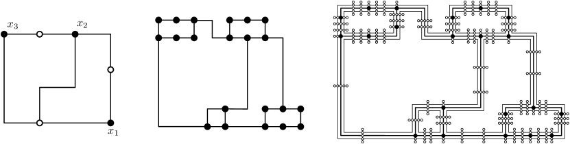
Figure 4: Left: incidence graph of $\phi=(x_{1}\vee\neg x_{2}\vee x_{3})\wedge(x_{1}\vee x_{2})\wedge(x_{2}\vee\neg x_{3})$ drawn in a grid. Middle: an instance of Vertex Cover where variables are replaced with length-$6$ variable cycles, and size-$3$ clauses are replaced with triangles. Right: adding a skeleton (see [26]) to get an instance of Connected Vertex Cover.

Initially, we mostly follow the first few steps of the connected vertex cover construction in [20]. Namely, refine this grid drawing by a factor of $4$, that is, we scale the drawing from the origin by a factor of $4$ while keeping the underlying grid unchanged. This allows us to replace the vertices corresponding to variables with cycles of length $6$, where the selection of odd or even vertices on the cycle corresponds to setting the variable to true or false. We connect graph edges corresponding to true literals to distinct even vertices and graph edges corresponding to false literals to distinct odd vertices. Each vertex corresponding to the size $3$ clause is replaced by a cycle of length $3$, with one incoming edge for each of the literals. For vertices corresponding to the size $2$ we subdivide one of the incident edges into a path of length $3$. Finally, vertices corresponding to the clauses of size one can be removed in a preprocessing step. Let $G^{*}_{2}$ be the resulting graph, which is drawn in an $\mathcal{O}(n)\times\mathcal{O}(n)$ grid. In particular, if $G^{*}_{2}$ has $n^{*}_{2}$ vertices, then $n^{*}_{2}=\mathcal{O}(n^{2})$.

Note that each variable cycle needs at least $3$ of its vertices in the vertex cover, each size-$3$ clause needs at least two vertices of its triangle in the vertex cover, and each size-$2$ clause needs at least two internal vertices of its path in the vertex cover. A size $3$-clause should be satisfied by some literal, which would mean that the edge corresponding to this literal would be covered from the variable cycle, and therefore it is sufficient to select the other two vertices of the triangle. In a size-$2$ clause at least one of the contained literals should be true, which exactly corresponds to the fact that one of the endpoints of the corresponding edge has to be selected. Since there is a path of length $5$ connecting these two vertices, we need to select the two odd or even index internal vertices from it. With these at hand, the following is a simple observation.

Lemma 6.6.

The formula $\phi_{2}$ has a satisfying assignment if and only if $G^{*}_{2}$ has a vertex cover of size $k^{*}_{2}=3n^{\prime}+2m^{\prime}=\mathcal{O}(n^{2})$, where $n^{\prime}$ and $m^{\prime}$ are the number of variables and size-$3$ clauses in $\phi_{2}$. If $G^{*}_{2}$ has a vertex cover of size $k^{*}_{2}+t$, then $\phi_{2}$ has an assignment that satisfies all but at most $9t$ clauses.

Proof.

If $\phi_{2}$ is satisfiable, then we select the true or false vertices on the variable cycles according to the assignment. In each clause, there is at least one literal that is true; we select the vertices on the clause cycle that correspond to the other two literals. The resulting set is clearly a vertex cover. On the other hand, every vertex cover must have at least $3n^{\prime}+2m^{\prime}$ vertices, as in order to cover the variable cycles and the clause triangles individually, one needs at least $3$ vertices per variable cycle and at least $2$ vertices per clause triangle. Such a vertex cover in addition will select only even or odd vertices from variable cycles, which yields a variable assignment that satisfies $\phi_{2}$.

If $G^{*}_{2}$ has a vertex cover of size $k^{*}_{2}+t$, then there can be at most $t$ variable cycles or clause triangles where the number of vertices selected is more than $3$ (respectively, $2$). Therefore we can mark "bad" any variable whose cycle has more than $3$ vertices or that appears in size-$3$ clause whose triangle has all vertices selected. Consequently, we have at most $3t$ bad variables. Since $3t$ variables can appear in at most $9t$ clauses, all but at most $9t$ clause triangles will have exactly two vertices selected. One can check that the assignment on the non-bad variables will then satisfy all but $9t$ clauses. ∎

As a final step for the planar construction, we introduce the skeleton described by Garey and Johnson [26]; this again requires that we refine the drawing by a constant factor. The procedure subdivides each edge of the graph twice, using $n_{sub}$ new vertices, and also adds $n_{skel}$ skeleton vertices. An important property of the skeleton is that the number of newly added vertices is $n_{skel}+n_{sub}=\Theta(|V(G^{*}_{2})|+|E(G^{*}_{2}|)=\mathcal{O}(n^{2})$. The resulting graph is drawn in an $\mathcal{O}(n)\times\mathcal{O}(n)$ grid. We use a final 4-refinement to ensure that inside the $\ell_{1}$-disk of radius $4$ around each vertex $v$ the only grid edges being used are on the horizontal or vertical line going through $v$. Let $G_{2}$ denote the resulting plane graph (i.e., the graph together with its embedding in the plane).

Lemma 6.7.

The graph $G^{*}_{2}$ has a vertex cover of size $k^{*}$ if and only if $G_{2}$ has a connected vertex cover of size $k_{2}:=k^{*}+(n_{skel}+n_{sub})/2$. If $G_{2}$ has a connected vertex cover of size $k_{2}+t$, then $G^{*}$ has a vertex cover of size $k^{*}+t$.

Proof.

The construction of Garey and Johnson [26] has the properties that (i) any connected vertex cover of $G_{2}$, when restricted to the vertices of $G^{*}_{2}$, is a vertex cover of $G^{*}_{2}$, and (ii) one can add $(n_{skel}+n_{sub})/2$ vertices among the subdivision and skeleton vertices to any vertex cover of $G^{*}_{2}$ to get a connected vertex cover of $G_{2}$. The first claim follows directly from the above properties. For the second claim, we note that the $n_{skel}$ skeleton vertices come in pairs, where one vertex in the pair has degree one and is connected only to the other vertex. Therefore, at least one vertex in each pair must be selected in every vertex cover. Similarly, the vertices in $n_{sub}$ also come in pairs, each pair being connected to each other, therefore one must select at least one vertex from each pair into any vertex cover. Now consider a connected vertex cover of size $k_{2}+t$ in $G_{2}$. Since there must be at least $(n_{skel}+n_{sub})/2$ vertices selected among the vertices newly introduced in $G_{2}$, there can be at most $k_{2}+t-(n_{skel}+n_{sub})/2=k^{*}+t$ vertices selected among the original vertices in $G^{*}_{2}$. It follows that $G^{*}_{2}$ has a vertex cover of size $k^{*}+t$. ∎

Grid embedding in $\mathbb{R}^{d}$ for $d\geqslant 3$.

We again start with the incidence graph $G$ of $\phi$, and let $L=|E(G)|$ denote the number of literal occurrences in $\phi$. Let $G^{*}$ be the graph where variable vertices are replaced with variable cycles and clause vertices by triangles (or for size $2$ clauses, paths) in the same manner as seen in $G^{*}_{2}$. We will now define a different type of skeleton for these graphs. First, we subdivide each edge of $G^{*}$ twice, that is, we remove the edge $vw$, add the vertices $u^{\prime},v^{\prime}$, and add the edges $uu^{\prime},u^{\prime}v^{\prime}$, and $v^{\prime}v$. Let $G^{**}$ be the resulting graph, and let $n^{**}$ denote the number of its vertices. Consider the disjoint union of $G^{**}$ and the cycle graph $C^{*}$ with $n^{**}$ vertices. For each vertex $v$ of $G^{**}$, we can associate a distinct vertex $v^{\prime}$ in the cycle, and we also create a new vertex $v^{\prime\prime}$. Finally, we add the edges $vv^{\prime}$ and $v^{\prime}v^{\prime\prime}$. It is routine to check that the resulting graph has $\mathcal{O}(n)$ vertices and $\mathcal{O}(n)$ edges, and it has maximum degree $4$. Therefore, we can apply the following theorem, which is paraphrased from [20].

Theorem 6.8 (Cube Wiring Theorem [20]).

There is a constant $c$ such that for any $d\geqslant 3$ it holds that any graph $G$ of maximum degree $2d$ on $n$ vertices can be drawn in a $d$-dimensional grid cube of side length $cn^{1/{d-1}}$. Moreover, given $G$ and $d$ the embedding can be constructed in polynomial time.

Since the graph has maximum degree $4<2d$ and $\mathcal{O}(n)$ vertices and edges, the resulting drawing is in a grid cube of side length $\mathcal{O}(n^{1/(d-1)})$. For a vertex $v$, let $\ell_{1}(v)$ and $\ell_{2}(v)$ be the lines that are parallel to the first and second coordinate axis respectively and pass through $v$. We use a constant-refinement and reorganize the neighborhood of each vertex $v$ in the grid drawing so that the grid edges used by the drawing in the $\ell_{1}$-ball of radius $4$ around $v$ all fall on $\ell_{1}$ and $\ell_{2}$. Let $G_{d}$ denote the resulting graph together with the obtained grid drawing.

One can prove the analogue of Lemma 6.6 for $G^{*}$ (with $\phi$ instead of $\phi_{2}$), and also the analogue of Lemma 6.7 for $G_{d}$.

Putting Lemmas 6.5, 6.6 and 6.7 together, and putting the higher dimensional analogues of Lemmas 6.6, 6.7 together, we get the following corollary, which is all that we will need from this subsection for the proof.

Corollary 6.9.

For each $d\geqslant 2$ the following holds. Given a $(3,3)$-CNF formula $\phi$ on $n$ variables, we can generate a graph $G_{d}$ of degree at most $4$ drawn in a $d$-dimensional grid of side length $O(n^{1/(d-1)})$ in polynomial time such that (a) if $\phi$ is satisfiable then $G_{d}$ has a connected vertex cover of size $k_{d}=\mathcal{O}(n^{d/(d-1)})$ and (b) if $G_{d}$ has a connected vertex cover of size $k_{d}+t$, then $\phi$ has an assignment satisfying all but $\mathcal{O}(t)$ clauses.

6.2.2 Construction and canonization

Given any graph $G_{d}$ that is drawn in a $d$-dimensional grid, we construct a point set $P_{d}$ the following way.

1. Refine the drawing of $G_{d}$ by a factor of $137$. (The constant $137$ will be justified in Lemma 6.13.)

2. Add all grid points that are internal to edges of $G_{d}$ to $P_{d}$.

3. Remove any point from $P_{d}$ that is at distance strictly less than $2$ from a vertex of $G_{d}$.

We call the set of points in $P_{d}$ that fall on an edge of $G_{d}$ edge components, and the $l_{1}$ balls of radius $2$ around vertices of $G_{d}$ are the cutouts. (The cutouts are cubes of diameter $4$ whose diagonals are axis-parallel; i.e., they are regular “diamonds” in $\mathbb{R}^{2}$.)

The resulting set $P_{d}$ is our construction for Rectilinear Steiner Tree. The following lemma can be found in [26], but we provide a proof for completeness.

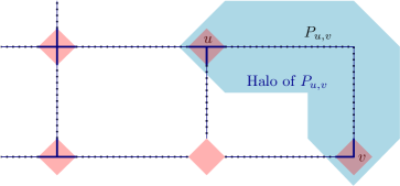
Figure 5: Construction of components from [26] in $\mathbb{R}^{2}$. Dotted edges are edge components, and the red rotated squares are the cutouts. The blue object represents the halo of the edge component $P_{u,v}$ in the top-right corner. Blue (thin and thick) edges correspond to the edges of a canonical Steiner tree.

Lemma 6.10 (Garey and Johnson [26]).

If $G_{d}$ has a connected vertex cover of size $k_{d}$, then $P_{d}$ has a rectilinear Steiner tree of total length $\ell_{d}:=L+2|E(G_{d})|+2(k_{d}-1)$, where $L$ is the total length of the edge components.

Proof.

Given a connected vertex cover $S$ of size $k_{d}$, we construct a Steiner tree $T$ the following way. First, we add all length $1$ edges connecting neighboring vertices in edge components to $T$; these have total length $L$. Since $S$ induces a connected graph, it has a spanning tree that has $k_{d}-1$ edges. The total length of these edges is $4(k_{d}-1)$. On each such edge component, we add the length $2$ edges that connect to the incident cutouts on both ends. Furthermore, on each edge $e$ of $G_{d}$ that is not an edge of this spanning tree, there is at least one endpoint $s$ of $e$ that is in $S$ as $S$ is a vertex cover. We add a length $2$ cutout edge connecting the edge component of $e$ to the center of the cutout of $s$. These edges have a total length of $2(|E(G_{d})|-k_{d}+1)$. The result is a tree $T$ on $P_{d}$ that has total length

$$L+4(k_{d}-1)+2(|E(G_{d})|-k_{d}+1)=L+2|E(G_{d})|+2(k_{d}-1).\qed$$

In the remainder of this subsection, we will canonize an approximate Steiner tree of $P_{d}$ in order to prove the following lemma.

Lemma 6.11.

If $P_{d}$ has a rectilinear Steiner tree of length $\ell_{d}+\ell^{\prime}$, then $G_{d}$ has a connected vertex cover of size $k_{d}+\ell^{\prime}/2$.

Canonization

We say that a Steiner tree of $P_{d}$ is canonical if (i) every length $1$ edge in edge components is included in $T$ and (ii) all other segments in $T$ have length $2$ and connect the center of some cutout to the nearest point in one of the incident edge components.

A Steiner point of $T$ is a point that has degree at least $3$. The vertices of $T$ are its Steiner points and $P_{d}$. An edge of $T$ is a curve connecting two vertices. It follows that $T$ has at most $|P_{d}|-2$ Steiner points.

For a fixed constant $d\geqslant 2$ we can change each edge of $T$ so that it is a minimum length path in the $\ell_{1}$ norm between these two vertices, by moving parallel to the $x_{1}$ axis, then to the $x_{2}$ axis, etc. until we arrive at the destination. The resulting tree consists of $\mathcal{O}(|P_{d}|)$ axis-parallel segments.

Lemma 6.12.

For any approximate Steiner tree $T$ on $P_{d}$ there is a Steiner tree $T^{\prime}$ so that it contains all length-$1$ edges in edge components and all of its edges have length at most $4$, and $T^{\prime}$ is no longer than $T$.

Proof.

Recall that the Hanan-grid [31] of $P_{d}$ is the set of points $H_{d}\subset\mathbb{R}^{d}$ that can be defined as the intersection of $d$ distinct axis-parallel hyperplanes incident to $d$ (not necessarily distinct) points of $P_{d}$. Snyder [51] shows that there exists a minimum rectilinear Steiner Tree whose Steiner points are on the Hanan-grid. In fact, he proposes modifications that are local, and can be applied also to a non-optimal Steiner tree, i.e., affect only a vertex of a Steiner tree and its neighbors, and result in a tree whose Steiner points lie on the Hanan-grid. None of the local modifications lengthen the tree. Moreover, each type of local modification either shortens $T$ by removing at least one segment, or it does not shorten the tree but it can be repeated no more than $\mathcal{O}(|P_{d}|)$ times. Consequently, given a tree $T$, we can use the local modifications of Snyder exhaustively to get a tree that is not longer than $T$, and whose Steiner points lie in the Hanan-grid of $P_{d}$.

Suppose now that $T$ is a rectilinear Steiner tree of $P_{d}$ whose Steiner points are in $H_{d}$. Notice that the minimum distance between points of $H_{d}$ is $1$, and the minimum distance between points from two distinct edge components is at least $4$. Suppose that there is an edge $uv$ of length $1$ in an edge component that is not in $T$. Then adding $uv$ to $T$ creates a cycle, and that cycle has at least one edge $e$ that has either length more than $1$, or $e$ has length exactly one but its endpoints are not covered by any edge component. Replacing $e$ with $uv$ therefore results in a tree that is no longer than $T$ and has one more length-$1$ edge that is inside an edge component. Repeating the above check $\mathcal{O}(|P_{d}|)$ times results in a tree $T$ that contains all length-$1$ edges in edge components. Suppose now that $T$ has an edge $uv$ of length more than $4$. Removing the edge $uv$ from $T$ creates a forest of two trees. Suppose that one tree spans $P\subset P_{d}$ and the other spans $Q\subset P_{d}$. Note that $P$ and $Q$ are non-empty, disjoint, and their union is $P_{d}$. Observe that there exists $p\in P$ and $q\in Q$ such that $\lVert p-q\rVert_{1}\leqslant 4$. Now the shortest edge connecting $p$ and $q$ is shorter than $e$ was, therefore by adding this edge the created tree is not longer than the original. As each such modification decreases the number of edges of length more than $4$ and there are only $\mathcal{O}(|P_{d}|)$ edges in $T$, we can remove all edges longer than $4$ in $\mathcal{O}(|P_{d}|^{2})$ time. The resulting tree $T^{\prime}$ satisfies the required properties. ∎

Lemma 6.13.

For any approximate Steiner tree $T^{\prime}$ on $P_{d}$ that contains all length-$1$ edges in edge components and no edges longer than $4$, there is a canonical tree $T^{\prime\prime}$ that is no longer than $T^{\prime}$.

Proof.

A full Steiner subtree of $T$ is a subtree of $T$ whose internal vertices are Steiner points of $T$, and whose leaves are points of $P_{d}$. Let $F$ be a full Steiner subtree of $T^{\prime}$ with $k$ leaves. The halo of an edge component $P_{uv}$ is the set of points in $\mathbb{R}^{d}$ whose $\ell_{1}$-distance from $P_{uv}$ is at most $68$. The refinement step of the construction of $P_{d}$ (see step (i)) ensures that two halos intersect if and only if the corresponding edges are incident to the same vertex.

Since $T^{\prime}$ contains all length-$1$ edges in edge components, the role of $F$ is to connect a certain set of edge components; each edge component contains at most one leaf of $F$ (as otherwise there would be a cycle). Let $\gamma$ be the number of edge components adjacent to $F$ in the tree, that is, $F$ has $\gamma$ leaves. Let $\beta$ be the number of Steiner points in $F$. Notice that $\beta<\gamma$.

First, we show that the leaves of $F$ are in edge components that are incident to the same cutout. Let $\mu$ be the number of pairs $(p,H)$ where $p$ is a Steiner point of $F$, and $H$ is a halo for one of the edge components connected to $F$, and moreover $p\in H$. On one hand, every Steiner point can be contained in at most $4$ halos, since that is the maximum overlap achieved by the halos. This is a consequence of the fact that halos corresponding to non-incident edge components are disjoint so any set of intersecting halos must correspond to the neighborhood of a single vertex, and the maximum degree of a vertex in $G_{d}$ is $4$. Therefore, we have that $\mu\leqslant 4\beta$.

On the other hand, since the maximum degree of $G_{d}$ is $4$, there is a set $E$ of at least $\gamma/4$ pairwise non-incident edge components; in particular, there is a point $r$ in $F$ that is outside all the closed halos corresponding to edge components in $E$. Let $r$ be the root of $F$, and for an edge component $P_{uv}\in E$, consider the unique path in $F$ from the leaf in $P_{u,v}$ to $r$. This path must intersect the halo of $P_{uv}$ at some point, and the portion of this path within the halo of $P_{uv}$ has length at least $68$. Notice that these paths are disjoint for each edge component of $F$. Since edges of $F$ have length at most $4$, there must be at least $68/4-1=16$ Steiner points on each such path, so altogether we have $\mu\geqslant(\gamma/4)\cdot 16=4\gamma$. Putting the upper and lower bound on $\mu$ together, we have that $4\gamma\leqslant 4\beta$. But this contradicts the fact that $\beta<\gamma$.

Consider now a full Steiner subtree $F$ that is connecting $\gamma\in\{2,3,4\}$ adjacent edge components. Then $F$ could have length $2\gamma$, as we can connect the point associated with the common vertex $v$ from the point set $P_{1}$ with length two segments to the nearest vertex of all the edge components connected by $F$. We show that this is the shortest possible tree for $\gamma$ edge components. Notice that any pair of edge components have $\ell_{1}$-distance exactly four, so the shortest path in the rectilinear Steiner tree between any pair of components is at least four. Now consider the geometric graph that we get by doubling every segment in the tree, so that we get parallel edges everywhere. This graph has an Euler tour (since every degree is even); on such an Euler tour, the length required between any pair of tree leaf vertices is at least the length of a shortest path between them, which is at least $4$. Since the length of the tour is exactly twice the length of the tree, we get that the tree has total length at least $4\gamma/2=2\gamma$, as claimed. Therefore, we can exchange each full Steiner subtree with a canonical connection. The resulting tree $T^{\prime\prime}$ is canonical and no longer than $T^{\prime}$. ∎

We can now prove the correspondence between an approximate rectilinear Steiner tree and a connected vertex cover.

Proof of Lemma 6.11.

Let $T$ be a Steiner tree of $P_{d}$ of length $\ell_{d}+\ell^{\prime}$. Using Lemma 6.12 and Lemma 6.13, we can create a canonical tree $T^{\prime\prime}$ in $n^{\mathcal{O}(1)}$ time of length at most $\ell_{d}+\ell^{\prime}$. Let $k$ be the number of non-empty cutouts. Observe that the vertices of $G_{d}$ corresponding to the non-empty cutouts form a connected vertex cover.

Consider the subtree $U$ of $T^{\prime\prime}$ that is spanned by the centers of the non-empty cutouts. Every edge component in $U$ must be connected to the centers of both neighboring cutouts, and $U$ contains $k-1$ edge components. Furthermore, every edge component outside $U$ must be connected to the center of at least one of the neighboring cutouts. Consequently, the length of $T^{\prime\prime}$ is at least $L+4(k-1)+2(|E(G_{d})|-k+1)=L+2|E(G_{d})|+2(k-1)$. Therefore, we have

$$L+2|E(G_{d})|+2(k-1)\leqslant\ell_{d}+\ell^{\prime}=L+2|E(G_{d})|+2(k_{d}-1)+\ell^{\prime},$$

and thus $k\leqslant k_{d}+\ell^{\prime}/2$, as required. ∎

6.2.3 Concluding the proof of Theorem 6.4

Proof of Theorem 6.4.

Putting Corollary 6.9 and Lemmas 6.10 and 6.11 together, we have that if a $(3,3)$-CNF formula $\phi$ on $n$ variables has a satisfying assignment then $P_{d}$ has a rectilinear Steiner tree of length $\ell_{d}=\mathcal{O}(n^{d/(d-1)})$. Let $c_{1}$ be such that $\ell_{d}=c_{1}n^{d/(d-1)}$. Additionally, if $P_{d}$ has a rectilinear Steiner tree of length $\ell_{d}+\ell^{\prime}$, then $\phi$ has an assignment that satisfies all but $c_{2}\ell^{\prime}$ clauses, where $c_{2}$ is a constant.

Suppose that there is a $2^{\gamma/\varepsilon^{d-1}}\mathrm{poly}(n)$ algorithm for Rectilinear Steiner Tree for all $\gamma>0$. Given a formula $\phi$, we create the set $P_{d}$ in polynomial time, and we run the above algorithm with $\varepsilon=\frac{\delta m}{c_{1}c_{2}n^{d/(d-1)}}$, where $m$ is the number of clauses in $\phi$. Since $m=\Theta(n)$, we have that $\varepsilon=\Theta(1/n^{1/(d-1)})$. We can now distinguish between a satisfiable formula (when a rectilinear Steiner tree on $P_{d}$ is of length $\ell_{d}$) and a formula in which all assignments violate at least $\delta m$ clauses (when any rectilinear Steiner tree on $P_{d}$ has length greater than $(1+\varepsilon)\ell_{d}$). Since the construction time of $P_{d}$ is polynomial in $n$, the total running time of this algorithm is $2^{\gamma/\varepsilon^{d-1}}\mathrm{poly}(n)=2^{\gamma cn}$ for some constant $c$. The existence of such algorithms for all $\gamma>0$ would therefore violate Gap-ETH by Corollary 6.1. ∎

7 Conclusion and Open Problems

In this article we gave randomized $(1+\varepsilon)$-approximation algorithms for Euclidean TSP, Euclidean Steiner Tree and Rectilinear Steiner Tree that run in $2^{\mathcal{O}(1/\varepsilon)^{d-1}}n+\mathrm{poly}(1/\varepsilon)n\log n$ time. In case of Euclidean TSP and Rectilinear Steiner Tree, we have shown that there are no $2^{o(1/\varepsilon)^{d-1}}\mathrm{poly}(n)$ algorithms under Gap-ETH. We achieved the improved algorithms by extending Arora’s method [1] with a new technique: Sparsity-Sensitive Patching.

As mentioned in the beginning of this paper, the methods from [1, 46] have been greatly generalized and extended to various other problems by several authors. A natural direction for further research would be to see whether Sparsity-Sensitive Patching can also be employed to obtain improved (and possibly, Gap-ETH-tight) approximation schemes for these problems. Examples of problems where such a question can be studied include

• Euclidean versions of Matching, $k$-TSP and $k$-Steiner Tree [1], Steiner Forest [11], $k$-Connectivity [16], $k$-Median [37, 5] and Survivable Network Design [17],

• versions of some of the above problems in other metric spaces (e.g., doubling, hyperbolic), and in planar, surface-embedded and minor free graphs (see Section 1.4 for such studies for TSP).

There are several open questions worth exploring further. The ideal algorithm for Euclidean TSP would have a running time of $2^{\mathcal{O}(1/\varepsilon)^{d-1}}n$, and it would be deterministic. However, achieving this running time with a randomized algorithm is already a challenging question. The most natural way to pursue this would be to try and unify Bartal and Gottlieb’s techniques [7] with ours. Is it possible to get this running time without spanners by using some new ideas to handle singletons (e.g., crossings that appear on their own on a facet of a quadtree cell)?

One could also pursue a $(1+\varepsilon)$-approximation algorithm that uses $f(1/\varepsilon)n^{\mathcal{O}(1)}$ time and only $\mathrm{poly}(1/\varepsilon,n)$ space, but this would likely require an algorithm that is not based on dynamic programming. Is such an algorithm possible (say, for $d=2$)?

Appendix A Filtering Algorithm

For a given set of points $P\subseteq\mathbb{R}^{d}$ let $\mathrm{ST}(P)$ be the minimum Steiner Tree with terminals $P$ and $\mathrm{MST}(P)$ be the minimum spanning tree of $P$. For any $X\subseteq\mathbb{R}^{d}$ let $\mathrm{ST}(P;X)$ be the¹⁵ minimum length Steiner Tree that connects terminals $P$ and is only allowed to use a subset of $X$ as Steiner Vertices (therefore $\mathrm{ST}(P;\mathbb{R}^{d})=\mathrm{ST}(P)$). We use $\mathcal{B}(\rho,R)$ to denote the ball centered in $\rho$ of radius $R$.

Definition A.1.

For any point sets $P_{0},P_{1}\subseteq\mathbb{R^{d}}$ we say that $X\subseteq P_{1}$ is an Steiner-filter of $P_{0}$ with respect to $P_{1}$ if:

1. $|X|\leqslant\frac{2^{\mathcal{O}(d^{4})}}{\varepsilon^{\mathcal{O}(1)}}|P_{0}|$, and

2. $\mathrm{wt}(\mathrm{ST}(P_{0};X))\leqslant(1+\varepsilon)\cdot\mathrm{wt}(\mathrm{ST}(P_{0};P_{1})$, and

3. $\mathrm{wt}(\mathrm{MST}(P_{0}\cup X))\leqslant\frac{2^{\mathcal{O}(d^{5})}}{\varepsilon^{\mathcal{O}(d)}}\cdot\mathrm{wt}(\mathrm{MST}(P_{0}))$.

In this section we prove the following filtering Lemma.

Lemma A.2.

For any point set $P\subset\mathbb{R}^{d}$ and any $\varepsilon>0$, there is an algorithm that:

1. finds a $X\subseteq\mathbb{R}^{d}$ that is a Steiner-filter of $P$ with respect to $\mathbb{R}^{d}$, and

2. runs in $\frac{2^{\mathcal{O}(d^{4})}}{\varepsilon^{\mathcal{O}(d)}}\cdot|P|+T_{\mathrm{spanner}}(|P|,\varepsilon)$ time.

The proof of our Lemma is based on the following, highly technical observation proved by Czumaj et al. [17].

Theorem A.3 (Lemma 4.1 from full version of [17]).

For any point sets $P_{0}$ and $P_{1}$ in $\mathbb{R}^{d}$ and any $\varepsilon>0$, there is an algorithm that finds a subset $X$ of $P_{0}$ that is a Steiner-filter of $P_{1}$ with respect to $P_{0}$ and runs in $(d/\varepsilon)^{\mathcal{O}(d)}n+T_{\mathrm{spanner}}(n)$, where $n=|P_{0}\cup P_{1}|$.

Algorithm : $\mathtt{Steiner-Filtering}(P)$, points $P\subseteq\mathbb{R}^{d}$ snapped to $L^{d}$ grid, where $L=\mathcal{O}(n/\varepsilon)$

1 Build a light $(1+\varepsilon)$-spanner $G$ on $P$

2  // Theorem 15.3.20 in [47]

3 foreach edge $e$ of $G$ do

4       $r_{e}:=\frac{2^{\mathcal{O}(d^{4})}}{\varepsilon}\cdot|e|$

5       Let $\mathrm{grid}(e)$ be the $d$-dimensional grid of side length $\frac{\varepsilon^{2}}{2^{\mathcal{O}(d^{3})}}\cdot|e|$

6       $X_{e}:=\mathrm{grid}(e)\cap\mathcal{B}(e,r_{e})$

return $X:=\bigcup_{e\in E[G]}X_{e}$

Algorithm 3 Pseudocode for the Steiner-Filtering algorithm of Czumaj et al. [17] when $P_{0}=\mathbb{R}^{d}$.

Observe that if we were to plug naively the set $P_{0}=\mathbb{R}^{d}$ into Theorem A.3 we would already prove Lemma A.2. Unfortunately, the running time of Theorem A.3 depends on $|P_{0}\cup P_{1}|$. For our purposes we only need to analyze their algorithm in the special case of $P_{0}=\mathbb{R}^{d}$. In Algorithm 3 we present the Steiner-filtering procedure of [17] in the special case of $P_{0}=\mathbb{R}^{d}$. First a light $(1+\varepsilon)$ spanner $G$ of $P$ is computed. Next, for every edge $e$ of the spanner $G$ a $d$-dimensional grid of side length $\varepsilon^{d}|e|/2^{\mathcal{O}(d^{3})}$ and radius $2^{\mathcal{O}(d^{4})}|e|/\varepsilon$ is determined in the middle-point of the edge $e$. Next this grid is added to $X$.

Now, we show that Algorithm 3 runs in $\frac{2^{\mathcal{O}(d^{4})}}{\varepsilon^{\mathcal{O}(d)}}|P|$ time.

Proof of Lemma A.2 (b).

To construct a light spanner $G$ we need $T_{\mathrm{spanner}}(|P|,\varepsilon)$ time (note that Algorithm 3 computes the spanner on $P$). Known constructions guarantee that the number of edges of such a spanner is bounded by $|P|/\varepsilon^{\mathcal{O}(d)}$ [17, 30, 47]. For any edge $e\in E[G]$, the number of grid points that we add to $X$ is bounded by $2^{\mathcal{O}(d^{4})}/\varepsilon^{\mathcal{O}(d)}$. The time needed to construct the grid around edge $e$ is bounded by $2^{\mathcal{O}(d^{4})}/\varepsilon^{\mathcal{O}(d)}$. Therefore the total runtime of Algorithm 3 is bounded by $T_{\mathrm{spanner}}(|P|,\varepsilon)+2^{\mathcal{O}(d^{4})}/\varepsilon^{\mathcal{O}(d)}|P|$. ∎

The correctness of Lemma A.2 (a) follows from the correctness of Theorem A.3. For completeness we sketch the arguments in Section A.1, making some simplifications that come from our specific setting.

A.1 $X$ is a Steiner-filter of $P$

Property (i) of $X$:

The set $X$ returned by Algorithm 3 satisfies property (i) of Definition A.1 because there are at most $|P|/\varepsilon^{\mathcal{O}(d)}$ edges of the spanner $G$ and for each edge we add at most $2^{\mathcal{O}(d^{4})}/\varepsilon^{\mathcal{O}(d)}$ many points.

Property (ii) of $X$:

Now we sketch the proof that $\mathrm{wt}(\mathrm{ST}(P;X))\leqslant(1+2\varepsilon)\cdot\mathrm{wt}(\mathrm{ST}(P;\mathbb{R}^{d}))$. Let $\mathcal{T}^{\ast}$ be a minimum Steiner tree of $P$ that can use any point in $\mathbb{R}^{d}$ as a Steiner point. We build a graph $H$ in three steps, consisting of edge sets $H_{1},H_{2}$ and $H_{3}$. The set $H_{1}$ consists of all the edges $(u,v)\in\mathcal{T}^{\ast}$ with $u,v\in P$. The set $H_{2}$ will be defined later; these edges are created from edges $(u,v)\in\mathcal{T}^{\ast}$ by moving the endpoints $(u,v)$ to $X$. Finally, the set $H_{3}$ makes $H$ connected by adding additional edges incident to the endpoints of $H_{1}\cup H_{2}$ that have total minimum weight.

Czumaj et al. [17] use $\mathcal{E}_{1}$ to denote the edges of $\mathcal{T}^{\ast}$ with both endpoints in $P$. Moreover, $\mathcal{E}_{2}$ are the edges of $\mathcal{T}^{\ast}$ that are transformed in the second phase into edges $H_{2}$ and $\mathcal{E}_{3}=\mathcal{T}^{\ast}\setminus(\mathcal{E}_{1}\cup\mathcal{E}_{2})$.

Clearly the graph $H$ is the spanning tree of $P$ that uses only points from $X$ as the Steiner vertices. We need to bound the total weight of $H$. Czumaj et al. [17] show that $\mathrm{wt}(H_{2})\leqslant\mathrm{wt}(\mathcal{E}_{2})+\varepsilon\cdot\mathrm{wt}(\mathcal{T}^{\ast})$ and $\mathrm{wt}(H_{3})\leqslant\mathrm{wt}(\mathcal{E}_{3})+\varepsilon\cdot\mathrm{wt}(\mathcal{T}^{\ast})$. Since $\mathrm{wt}(H_{1})=\mathrm{wt}(\mathcal{E}_{1})$ this leads to:

$$\mathrm{wt}(H) \leqslant\mathrm{wt}(H_{1})+\mathrm{wt}(H_{2})+\mathrm{wt}(H_{3})$$

$$\leqslant\mathrm{wt}(\mathcal{E}_{1})+(\mathrm{wt}(\mathcal{E}_{2})+\varepsilon\mathrm{wt}(\mathcal{T}^{\ast}))+(\mathrm{wt}(\mathcal{E}_{3})+\varepsilon\mathrm{wt}(\mathcal{T}^{\ast}))$$

$$\leqslant(1+2\varepsilon)\mathrm{wt}(\mathcal{T}^{\ast}).$$

We now expand on the construction of $H_{2}$ and $H_{3}$ and sketch the main ideas behind their arguments.

Bound on $\mathrm{wt}(H_{2})$:

Since the edge $(u,v)\in\mathcal{T}^{\ast}$ is not in $\mathcal{E}_{1}$ either $u$ or $v$ are not in $P$. Let $t$ be the middle point of $(u,v)$. We will add $(u,v)$ to $\mathcal{E}_{2}$ if there are two points $x,y\in P$ that are (i) disconnected in $\mathcal{T}^{\ast}$ after removing edge $(u,v)$ and (ii) the shortest path $p_{x\leadsto y}$ in the spanner $G$ is fully contained in $\mathcal{B}(t,2^{\mathcal{O}(d^{3})}\mathrm{dist}(u,v)/\varepsilon)$.

Next Czumaj et al. [17] show that there exists an edge $e$ on $p_{x\leadsto y}$ whose length is at least $|e|\geqslant\mathrm{dist}(u,v)$.

Claim A.4 (Lemma 4.6 in [17]).

For a given $P\subseteq\mathbb{R}^{d}$ let $x,y$ be any pair of distinct points in $P$. Let $e$ be any edge in $\mathrm{ST}(P)$, such that after removal of $e$ from $\mathrm{ST}(P)$ the terminals $x$ and $y$ are in two different subtrees $T_{1}$ and $T_{2}$ of $\mathrm{ST}(P)$ respectively.

Suppose that $G$ is a connected graph on $P$ (for example $G$ is a spanner of $P$) and $p_{x\leadsto y}$ is the shortest path in $G$ from $x$ to $y$. Then at least one edge of $\mathrm{ST}(P)$ is not shorter than $|e|$.

Proof.

Suppose for the sake of contradiction that all edges on $p_{x\leadsto y}$ are shorter than $|e|$. Because $x$ and $y$ are in two different components there must exist an edge $e^{\prime}\in\mathrm{ST}(P)$ such that its endpoints are in different components and $|e^{\prime}|<|e|$. This means that $T_{1}\cup T_{2}\cup\{e\}$ is a Steiner tree of $P$ and has smaller length than $\mathrm{ST}(P)$, which contradicts the minimality of $\mathrm{ST}(P)$. ∎

This means that by the construction of $X$, there must exist two points $u^{\ast}$ and $v^{\ast}$ in $P\cup X$, such that $\mathrm{dist}(u,u^{\ast})$ and $\mathrm{dist}(v,v^{\ast})$ are at most $\varepsilon^{2}|e|/2^{\mathcal{O}(d^{3})}$. We modify $\mathcal{T}^{\ast}$ by moving all edges incident to $u$ and $v$ to have their endpoints at $u^{\ast}$ and $v^{\ast}$ (the number of such edges is at most some constant for fixed $d$). The additive increase due to selecting $u^{\ast}$ instead of $u$ and $v^{\ast}$ instead of $v$ is at most $\varepsilon^{2}/2^{\mathcal{O}(d^{3})}\cdot|e|\leqslant\varepsilon^{2}/2^{\mathcal{O}(d^{3})}\cdot\left(2^{\mathcal{O}(d^{3})}\mathrm{dist}(u,v)/\varepsilon\right)\leqslant\varepsilon\cdot\mathrm{dist}(u,v)$.

To summarize the total cost of the edges in $H_{2}$ is bounded by $\mathrm{wt}(\mathcal{E}_{2})+\sum_{(u,v)\in\mathcal{T}^{\ast}}\varepsilon\cdot\mathrm{dist}(u,v)\leqslant\mathrm{wt}(\mathcal{E}_{2})+\varepsilon\mathrm{wt}(\mathcal{T}^{\ast})$.

Bound on $\mathrm{wt}(H_{3})$:

Consider removing edge $(u,v)\in\mathrm{ST}(P)$ from $\mathrm{ST}(P)$. Let $\mathrm{ST}_{u}(P)$ and $\mathrm{ST}_{v}(P)$ denote the resulting trees containing $u$ and $v$ respectively. Let $T_{u}^{k}$ be the subtree of $\mathrm{ST}_{u}(P)$ induced by the vertices that are at a distance at most $k$ from $u$ for some parameter $k=\Theta(d^{2})$. Similarly let us define $T_{v}^{k}$ to be a subtree of $\mathrm{ST}_{v}(P)$ of vertices at hop-distance $k$ from $v$.

Consider an edge $(u,v)\in\mathcal{E}_{3}$. Because $(u,v)\notin\mathcal{E}_{1}\cup\mathcal{E}_{2}$ at least one of the following conditions hold: (i) either $T_{u}^{k}$ or $T_{v}^{k}$ contains an edge of length greater than $2^{\mathcal{O}(d^{3})}\mathrm{dist}(u,v)/\varepsilon$, or (ii) $\mathrm{ST}_{v}(P)$ or $\mathrm{ST}_{v}(P)$ has no endpoint in the ball $\mathcal{B}(t,2^{\mathcal{O}(d^{3})}\mathrm{dist}(u,v)/\varepsilon)$ (where $t$ is the midpoint of edge $(u,v)$).

Czumaj et al. [17] show that when $(u,v)\in\mathcal{E}_{3}$ then in the close proximity of $(u,v)$ there is a long edge (see Observation A.7). They show it by combining the following claims:

Claim A.5 (Lemma 4.6 in [17]).

For any $P,X\subseteq\mathbb{R}^{d}$ let $T$ be any subtree of $\mathrm{ST}(P;X)$ and let $P^{\prime}$ be the set of leaves of $T$. Then $T=\mathrm{ST}(P^{\prime};X)$.

Proof.

For the sake of contradiction assume that $T^{\ast}=\mathrm{ST}(P^{\prime},X)$ and $\mathrm{wt}(T^{\ast})$ is smaller than $\mathrm{wt}(T)$. We replace the tree $T$ by the tree $T^{\ast}$ in $\mathrm{ST}(P,X)$. We get a graph of weight smaller than $\mathrm{ST}(P;X)$ that contains a Steiner Tree of $P$ and uses only $X$ as a Steiner points. However, this graph has smaller weight than $\mathrm{ST}(P;X)$ which implies a contradiction. ∎

Claim A.6 (Lemma 4.8 in [17]).

Let $P,X\subseteq\mathbb{R}^{d}$. For any $\rho_{0}\in\mathbb{R}^{d}$ if $\mathrm{ST}(P;X)\cap\mathcal{B}(\rho_{0},1)$ contains at most $1$ terminal from $P$, then for any $\alpha\in(0,1)$ the $\mathrm{ST}(P;X)\cap\mathcal{B}(\rho_{0},\alpha)$ contains at most $2^{\mathcal{O}(d^{2})}$ Steiner points from $X$.

The proof of Claim A.6 is technical, but it also works in the $\ell_{1}$ norm. An analogous claim is also proven in [50, Lemma 36]. We skip the proof of Claim A.6. Note that $k$ will be set to $cd^{2}$ where $c$ is chosen so that $2^{cd^{2}}$ is strictly larger than the bound on Steiner points guaranteed by Claim A.6 for $\alpha=1/2$.

Observation A.7.

If $(u,v)\in\mathcal{E}_{3}$ then there is an edge $(u^{\ast},v^{\ast})\in T_{u}^{k}\cup T_{v}^{k}$ of length at least $2^{\mathcal{O}(d^{3})}\mathrm{dist}(u,v)/(k\varepsilon)$.

Proof.

Fix $R:=2^{\mathcal{O}(d^{3})}\mathrm{dist}(u,v)/\varepsilon$. Since $(u,v)\not\in\mathcal{E}_{1}\cup\mathcal{E}_{2}$, we have that $\mathrm{ST}_{u}(P)\cap\mathcal{B}(t,R)$ or $\mathrm{ST}_{v}(P)\cap\mathcal{B}(t,R)$ is empty of terminals (other than $u,v$). Without loss of generality, assume that $P\cap\mathrm{ST}_{u}(P)\cap\mathcal{B}(t,R)=\{u\}$. Suppose for the sake of contradiction that all edges in $T_{u}^{k}$ are smaller than $R/2k$. Then, $T_{u}^{k}$ must by fully contained in $\mathcal{B}(t,R/2)$. Since there are no terminals in $\mathcal{B}(t,R)$ other than $u$, the tree $T_{u}^{k}$ must contain at least $2^{k}$ Steiner points. Note that $\mathrm{ST}_{u}(P)$ is a Steiner tree of its leaves by Claim A.5. Now applying Claim A.6 to $\mathrm{ST}_{u}(P)$ and the balls $\mathcal{B}(t,R)$ and $\mathcal{B}(t,R/2)$ leads to a contradiction, as $\mathcal{B}(t,R/2)$ has at least $2^{k}$ Steiner points. ∎

Czumaj et al. [17] charge the cost of the edge $(u,v)\in\mathcal{E}_{3}$ to the edge $(u^{\ast},v^{\ast})\in T_{u}\cup T_{v}$ guaranteed by Observation A.7 in order to bound the cost of edges in $H_{3}$. They design their charging scheme in such a way that the total cost of all edges charged to $e$ is upper bounded by $\varepsilon|e|$.

To analyze the charging scheme observe that an edge can be charged to $e\in\mathcal{T}^{\ast}$ only if it is at most $(k-1)$-hop distance from one of the endpoints of $e$. The number of such edges is at most $4\Delta^{k}$ (where $\Delta\leqslant 2^{\mathcal{O}(d)}$ is the maximum degree of any minimum spanning tree in $\mathcal{R}^{d}$). Moreover, the lengths of such edges are upper bounded by $\varepsilon|e|/(4\Delta^{k})$: by Observation A.7 an edge $(u,v)$ is charged to $(u^{\ast},v^{\ast})$ only if $\mathrm{dist}(u,v)\geqslant 2^{\mathcal{O}(d^{3})}\mathrm{dist}(u,v)/(k\varepsilon)$ and we select $k=cd^{2}$ for a large enough constant $c$. This shows that $\mathrm{wt}(\mathcal{E}_{3})\leqslant\varepsilon\mathrm{wt}(T^{\ast})$.

Next, they observe that $\mathcal{E}_{3}$ induces a forest. Let $T^{\prime}$ be any tree in this forest and let $V^{\prime}$ be the set of vertices in $T^{\prime}$ belonging to $P$. Czumaj et al. [17] take any minimum spanning tree on $V^{\prime}$ and add it to $H_{3}$. Because the cost of the minimum spanning tree on $V^{\prime}$ is at most twice the cost of $\mathrm{wt}(\mathrm{ST}(V^{\prime}))\leqslant\mathrm{wt}(T^{\prime})$ it shows that $\mathrm{wt}(H_{3})\leqslant 2\mathrm{wt}(\mathcal{E}_{3})$ and therefore $\mathrm{wt}(H_{3})\leqslant\mathrm{wt}(\mathcal{E}_{3})+\varepsilon\mathrm{wt}(T^{\ast})$.

Property (iii) of $X$:

Now, we prove property (iii) of $X$, namely that $\mathrm{wt}(\mathrm{MST}(P\cup X))\leqslant 2^{\mathcal{O}(d^{4})}/\varepsilon^{\mathcal{O}(d)}\cdot\mathrm{wt}(\mathrm{MST}(P))$ (see Lemma 4.10 in the full version of [17]). We construct a spanning graph $\mathcal{T}$ of $P\cup X$. First we take $\mathcal{T}$ to be the minimum spanning tree of $P$. Next for every edge $e\in G$ we find a minimum spanning tree $\mathcal{T}_{e}$ of $X_{e}$ and connect it to any of the endpoints of $e$. Such a graph is a spanning graph of $P\cup X$. Now we focus on estimating the cost of $\mathcal{T}$.

Fix an arbitrarily edge $e$ in $G$. By definition all the points in $X_{e}$ are grid points within distance $r_{e}=\frac{2^{\mathcal{O}(d^{4})}}{\varepsilon}\cdot|e|$ from the midpoint of $e$. Since the grid has side length $\mu=\frac{\varepsilon^{2}}{2^{\mathcal{O}(d^{3})}}\cdot|e|$, we get that $|X_{e}|=O(r_{e}/\mu)^{d}$. Therefore the total length of the minimum spanning tree of $\mathcal{T}_{e}$ is:

$$O(|X_{e}|\cdot\mu)=O(r_{e}^{d}/\mu^{d-1})=\frac{2^{\mathcal{O}(d^{5})}}{\varepsilon^{\mathcal{O}(d)}}|e|.$$

Hence, the total cost of $\mathcal{T}$ is bounded by

$$\mathrm{wt}(\mathrm{MST}(P))+\sum_{e\in E[G]}\frac{2^{\mathcal{O}(d^{5})}}{\varepsilon^{\mathcal{O}(d)}}\cdot|e|\leqslant\frac{2^{\mathcal{O}(d^{5})}}{\varepsilon^{\mathcal{O}(d)}}\cdot\mathrm{wt}(G)\leqslant\frac{2^{\mathcal{O}(d^{5})}}{\varepsilon^{\mathcal{O}(d)}}\cdot\mathrm{wt}(\mathrm{MST}(P))$$

This concludes the proof of property (iii) of the set $X$ and proof of Lemma A.2.

A.2 Proof of Lemma 5.7

Now, we proceed with the proof of Lemma 5.7. Recall that we are given a point set $P$ and a random offset $\mathbf{a}$. The task is to find a set $\tilde{S}$ of segments with the property that (i) there is a Steiner tree that uses $\tilde{S}$ which is a $(1+\varepsilon)$-approximation of the optimum solution and (ii) it has at most $(1/\varepsilon)^{\mathcal{O}(d)}$ crossings with each facet of the quadtree.

We use the Filtering Lemma A.2 and get a set $X\subseteq\mathbb{R}^{d}$, with the property that $\mathrm{ST}(P;X)$ is a $(1+\varepsilon)$-approximation of $\mathrm{ST}(P)$ and $\mathrm{MST}(P\cup X)\leqslant\frac{2^{\mathcal{O}(d^{5})}}{\varepsilon^{\mathcal{O}(d)}}\cdot\mathrm{MST}(P)$. Next, we compute a graph $G$ that is a light $(1+\varepsilon)$-spanner of $P\cup X$. Here, we use a spanner construction due to [25] that guarantees a light spanner in doubling metrics (to make it work both in Euclidean and Rectilinear Space) and works in $\mathcal{O}(n\log(n))$ time.

The graph $G$ has weight $\mathrm{poly}(1/\varepsilon)\mathrm{MST}(P)$ and there is a $(1+\mathcal{O}(\varepsilon)$-approximate Steiner tree on $P$ that uses only the edges of $G$. Now, we need to guarantee that edges of $G$ are crossing each facet of a quadtree at most $(1/\varepsilon)^{\mathcal{O}(d)}$ times. To achieve that we use the lightening procedure of Rao and Smith [50] (see Lemma 5.1). Their lightening procedure works for any connected graph (see also the lightening procedures in [17, 16] and [47, Lemma 19.3.2]).

This gives us a graph $\tilde{G}$ with $\mathrm{wt}(\tilde{G})-\mathrm{wt}(G)\leqslant\varepsilon\mathrm{wt}(\mathrm{ST}(P))$, it contains a Steiner tree on $P$ that is only $(1+\mathcal{O}(\varepsilon))$-times heavier than $\mathrm{ST}(P)$, and each facet of the quadtree is crossed by $\tilde{G}$ at most $(1/\varepsilon)^{\mathcal{O}(d)}$ times. The set $\tilde{S}$ consists of the edges of $\tilde{G}$. This concludes the proof of Lemma 5.7.

References

- [1] S. Arora. Polynomial Time Approximation Schemes for Euclidean Traveling Salesman and other Geometric Problems. J. ACM, 45(5):753–782, 1998.
- [2] S. Arora. Approximation schemes for NP-hard geometric optimization problems: a survey. Math. Program., 97(1-2):43–69, 2003.
- [3] S. Arora, M. Grigni, D. R. Karger, P. N. Klein, and A. Woloszyn. A polynomial-time approximation scheme for weighted planar graph TSP. In Proceedings of the Ninth Annual ACM-SIAM Symposium on Discrete Algorithms, 25-27 January 1998, San Francisco, California, USA, pages 33–41, 1998.
- [4] S. Arora, M. Grigni, D. R. Karger, P. N. Klein, and A. Woloszyn. A polynomial-time approximation scheme for weighted planar graph TSP. In Proceedings of the Ninth Annual ACM-SIAM Symposium on Discrete Algorithms (SODA 1998), pages 33–41, 1998.
- [5] S. Arora, P. Raghavan, and S. Rao. Approximation Schemes for Euclidean k-Medians and Related Problems. In Proceedings of the Thirtieth Annual ACM Symposium on the Theory of Computing, 1998, pages 106–113, 1998.
- [6] B. S. Baker. Approximation Algorithms for NP-Complete Problems on Planar Graphs. J. ACM, 41(1):153–180, 1994.
- [7] Y. Bartal and L. Gottlieb. A Linear Time Approximation Scheme for Euclidean TSP. In 54th Annual IEEE Symposium on Foundations of Computer Science (FOCS 2013), pages 698–706. IEEE Computer Society, 2013.
- [8] Y. Bartal, L. Gottlieb, and R. Krauthgamer. The Traveling Salesman Problem: Low-Dimensionality Implies a Polynomial Time Approximation Scheme. SIAM J. Comput., 45(4):1563–1581, 2016.
- [9] S. Bhore and C. D. Tóth. Light Euclidean Steiner Spanners in the Plane. In 37th International Symposium on Computational Geometry (SoCG 2021), volume 189, pages 15:1–15:17, 2021.
- [10] H. L. Bodlaender, M. Cygan, S. Kratsch, and J. Nederlof. Deterministic single exponential time algorithms for connectivity problems parameterized by treewidth. Inf. Comput., 243:86–111, 2015.
- [11] G. Borradaile, P. N. Klein, and C. Mathieu. A Polynomial-Time Approximation Scheme for Euclidean Steiner Forest. ACM Trans. Algorithms, 11(3):19:1–19:20, 2015.
- [12] G. Borradaile, H. Le, and C. Wulff-Nilsen. Minor-free graphs have light spanners. In 58th IEEE Annual Symposium on Foundations of Computer Science (FOCS 2017), pages 767–778. IEEE Computer Society, 2017.
- [13] T. H. Chan and S. H. Jiang. Reducing curse of dimensionality: Improved PTAS for TSP (with neighborhoods) in doubling metrics. ACM Trans. Algorithms, 14(1):9:1–9:18, 2018.
- [14] L. Chen, K. Jansen, and G. Zhang. On the optimality of exact and approximation algorithms for scheduling problems. J. Comput. Syst. Sci., 96:1–32, 2018.
- [15] M. Cygan, S. Kratsch, and J. Nederlof. Fast Hamiltonicity Checking Via Bases of Perfect Matchings. J. ACM, 65(3):12:1–12:46, 2018.
- [16] A. Czumaj and A. Lingas. A Polynomial Time Approximation Scheme for Euclidean Minimum Cost k-Connectivity. In Automata, Languages and Programming, 25th International Colloquium (ICALP 1998), pages 682–694, 1998.
- [17] A. Czumaj, A. Lingas, and H. Zhao. Polynomial-Time Approximation Schemes for the Euclidean Survivable Network Design Problem. In Automata, Languages and Programming, 29th International Colloquium (ICALP 2002), pages 973–984, 2002.
- [18] G. Das, S. Kapoor, and M. H. M. Smid. On the Complexity of Approximating Euclidean Traveling Salesman Tours and Minimum Spanning Trees. Algorithmica, 19(4):447–460, 1997.
- [19] M. de Berg, H. L. Bodlaender, S. Kisfaludi-Bak, and S. Kolay. An ETH-tight exact algorithm for Euclidean TSP. In Proceedings of the 59th IEEE Annual Symposium on Foundations of Computer Science (FOCS 2018), pages 450–461. IEEE Computer Society, 2018.
- [20] M. de Berg, H. L. Bodlaender, S. Kisfaludi-Bak, D. Marx, and T. C. van der Zanden. A Framework for Exponential-Time-Hypothesis-Tight Algorithms and Lower Bounds in Geometric Intersection Graphs. SIAM J. Comput., 49(6):1291–1331, 2020.
- [21] E. D. Demaine, M. Hajiaghayi, and K. Kawarabayashi. Contraction Decomposition in H-Minor-Free Graphs and Algorithmic Applications. In Proceedings of the 43rd ACM Symposium on Theory of Computing (STOC 2011), pages 441–450, 2011.
- [22] I. Dinur. Mildly exponential reduction from gap 3SAT to polynomial-gap label-cover. Electron. Colloquium Comput. Complex., 23:128, 2016.
- [23] S. E. Dreyfus and R. A. Wagner. The Steiner problem in graphs. Networks, 1(3):195–207, 1971.
- [24] A. E. Feldmann, Karthik C. S., E. Lee, and P. Manurangsi. A survey on approximation in parameterized complexity: Hardness and algorithms. Algorithms, 13(6):146, 2020.
- [25] A. Filtser and S. Solomon. The greedy spanner is existentially optimal. SIAM J. Comput., 49(2):429–447, 2020.
- [26] M. R. Garey and D. S. Johnson. The rectilinear steiner tree problem is NP-complete. SIAM Journal on Applied Mathematics, 32(4):826–834, 1977.
- [27] L. Gottlieb and Y. Bartal. Near-linear time approximation schemes for Steiner tree and forest in low-dimensional spaces. Accepted to STOC 2021.
- [28] M. Grigni, E. Koutsoupias, and C. H. Papadimitriou. An approximation scheme for planar graph TSP. In 36th Annual Symposium on Foundations of Computer Science, Milwaukee, Wisconsin, USA, 23-25 October 1995, pages 640–645, 1995.
- [29] M. Grigni, E. Koutsoupias, and C. H. Papadimitriou. An approximation scheme for planar graph TSP. In 36th Annual Symposium on Foundations of Computer Science (FOCS 1995), pages 640–645, 1995.
- [30] J. Gudmundsson, C. Levcopoulos, and G. Narasimhan. Fast greedy algorithms for constructing sparse geometric spanners. SIAM J. Comput., 31(5):1479–1500, 2002.
- [31] M. Hanan. On Steiner’s problem with rectilinear distance. SIAM Journal on Applied Mathematics, 14(2):255–265, 1966.
- [32] S. Har-Peled. Geometric Approximation Algorithms. American Mathematical Society, USA, 2011.
- [33] A. Itai, C. H. Papadimitriou, and J. L. Szwarcfiter. Hamilton Paths in Grid Graphs. SIAM Journal on Computing, 11(4):676–686, 1982.
- [34] S. Kisfaludi-Bak. ETH-Tight Algorithms for Geometric Network Problems. PhD thesis, Technische Universiteit Eindhoven, Department of Mathematics and Computer Science, June 2019.
- [35] P. N. Klein. A Subset Spanner for Planar Graphs, with Application to Subset TSP. In Proceedings of the 38th Annual ACM Symposium on Theory of Computing (STOC 2006), pages 749–756, 2006.
- [36] P. N. Klein. A linear-time approximation scheme for TSP in undirected planar graphs with edge-weights. SIAM J. Comput., 37(6):1926–1952, 2008.
- [37] S. G. Kolliopoulos and S. Rao. A Nearly Linear-Time Approximation Scheme for the Euclidean k-Median Problem. SIAM J. Comput., 37(3):757–782, 2007.
- [38] B. Korte and J. Vygen. Combinatorial Optimization: Theory and Algorithms. Springer Publishing Company, Incorporated, 5th edition, 2012.
- [39] R. Krauthgamer and J. R. Lee. Algorithms on negatively curved spaces. In 47th Annual IEEE Symposium on Foundations of Computer Science (FOCS 2006), pages 119–132. IEEE Computer Society, 2006.
- [40] H. Le. A PTAS for subset TSP in minor-free graphs. In Proceedings of the 2020 ACM-SIAM Symposium on Discrete Algorithms (SODA 2020), pages 2279–2298, 2020.
- [41] H. Le and S. Solomon. Truly optimal euclidean spanners. In 60th IEEE Annual Symposium on Foundations of Computer Science (FOCS 2019), pages 1078–1100, 2019.
- [42] H. Le and S. Solomon. Light Euclidean Spanners with Steiner Points. In 28th Annual European Symposium on Algorithms (ESA 2020), pages 67:1–67:22, 2020.
- [43] D. Lichtenstein. Planar formulae and their uses. SIAM J. Comput., 11(2):329–343, 1982.
- [44] P. Manurangsi and P. Raghavendra. A Birthday Repetition Theorem and Complexity of Approximating Dense CSPs. In 44th International Colloquium on Automata, Languages, and Programming (ICALP 2017), pages 78:1–78:15, 2017.
- [45] D. Marx. On the optimality of planar and geometric approximation schemes. In 48th Annual IEEE Symposium on Foundations of Computer Science (FOCS 2007), pages 338–348, 2007.
- [46] J. S. B. Mitchell. Guillotine subdivisions approximate polygonal subdivisions: A simple polynomial-time approximation scheme for geometric TSP, k-MST, and related problems. SIAM Journal on Computing, 28(4):1298–1309, 1999.
- [47] G. Narasimhan and M. H. M. Smid. Geometric Spanner Networks. Cambridge University Press, 2007.
- [48] C. H. Papadimitriou. Computational Complexity. Addison-Wesley, 1994.
- [49] J. Plesník. The NP-Completeness of the Hamiltonian Cycle Problem in Planar Diagraphs with Degree Bound Two. Information Processing Letters, 8(4):199–201, 1979.
- [50] S. Rao and W. D. Smith. Approximating Geometrical Graphs via "Spanners" and "Banyans". In Proceedings of the Thirtieth Annual ACM Symposium on the Theory of Computing (STOC 1998), pages 540–550. ACM, 1998.
- [51] T. L. Snyder. On the Exact Location of Steiner Points in General Dimension. SIAM J. Comput., 21(1):163–180, 1992.
- [52] L. Trevisan. When Hamming Meets Euclid: The Approximability of Geometric TSP and Steiner Tree. SIAM J. Comput., 30(2):475–485, 2000.
- [53] V. V. Vazirani. Approximation Algorithms. Springer, 2004.
- [54] D. P. Williamson and D. B. Shmoys. The Design of Approximation Algorithms. Cambridge University Press, 2011.