Classification of Pulsars using Extreme Deconvolution

Abstract

We carry out a classification of the observed pulsar dataset into distinct clusters, based on the $P-\dot{P}$ diagram, using Extreme Deconvolution based Gaussian Mixture Model. We then use the Bayesian Information Criterion to select the optimum number of clusters. We find in accord with previous works, that the pulsar dataset can be optimally classified into six clusters, with two for the millisecond pulsar population, and four for the ordinary pulsar population. Beyond that, however we do not glean any additional insight into the pulsar population based on this classification. Using numerical experiments, we confirm that Extreme Deconvolution-based classification is less sensitive to variations in the dataset compared to ordinary Gaussian Mixture Models. All our analysis codes used for this work have been made publicly available.

1 Introduction

Neutron stars most commonly manifest themselves as radio pulsars. Pulsars are rotating neutron stars which emit pulsed radio emission. The zeroth-order model to explain the pulsed radio emission in pulsars is attributed to a rotating magnetic dipole, although the full details of the pulsar emission are much more complex and still not completely understood (Melrose et al., 2021). Ever since their first serendipitous discovery of a pulsar (neutron star) (Hewish et al., 1968), a whole zoo of neutron stars with considerable diversity have been discovered throughout the electromagnetic spectrum. Pulsars have proved to be wonderful laboratories for a wide range of topics in Physics and Astronomy (Lorimer & Kramer, 2012). A few representative examples of these myriad connections of pulsars to the rest of Physics/Astrophysics include: Solid state physics (Bhattacharya & van den Heuvel, 1991), Plasma Physics and Fluid Mechanics (Blandford, 1992), QED (Meszaros, 1992), QCD (Alford et al., 2008) tests of General Relativity (Stairs, 2003), study of nuclear matter at high densities (Lattimer, 2012; Bagchi, 2018), indirect probes of gravitational waves (Taylor, 1994), exoplanets (Wolszczan & Frail, 1992), dark matter (Desai & Kahya, 2016), stellar evolution (Stairs, 2004), probes of interstellar medium (Frail et al., 1994; Keith et al., 2013), solar wind (Krishnakumar et al., 2021) etc.

The two main observables which typically characterize a radio pulsar are its period ($P$) and period derivative ($\dot{P}$). From these, one can obtain approximate estimates of their ages and magnetic fields. Radio pulsars can be broadly classified into two types. The first category is ordinary radio pulsars with periods greater than approximately 100 ms, $\dot{P}$ between $10^{-16}$ and $10^{-13}$, and magnetic fields between $10^{10}-10^{13}$ G. Most of these pulsars are in isolated systems and the youngest of them are usually associated with supernova remnants. The second category is millisecond pulsars, with periods shorter than approximately 100 ms and characteristic surface magnetic field $<10^{10}$ G. The origin of these pulsars is different from the classical radio pulsar population, and these are generally accepted to be the descendants of low-mass X-ray binaries (Bhattacharya & van den Heuvel, 1991). More than 250 millisecond pulsars have also been discovered in gamma rays by the Fermi-LAT satellite, some of which are new discoveries, and have not yet been detected in the radio (Acero et al., 2015). As of now, the total number of known pulsars is close to 3,000 and we expect to discover about 20,000 new pulsars in the SKA era (Kramer & Stappers, 2015).

Subsequently, a whole zoo of neutron stars with diverse characteristics (Konar, 2017; Kaspi, 2010; Harding, 2013) have since been discovered, such as magnetars (Woods & Thompson, 2006), rotating radio transients (McLaughlin et al., 2006), X-ray dim isolated neutron stars (Mereghetti, 2011), Fast Radio bursts (Cordes & Chatterjee, 2019), Central compact objects (De Luca, 2017). Because of the proliferation of distinct observational classes of neutron stars, a number of automated techniques have been used to classify the pulsar population into distinct classes, in the hope of gaining new insights into the connection between these classes. The first class of techniques involve the study of evolutionary tracks along the $P$-$\dot{P}$ diagram, also known as “pulsar current” analysis (Vivekanand & Narayan, 1981; Vranešević & Melrose, 2011; Glushak, 2020). The second group of efforts involves the application of unsupervised clustering techniques. The first work along these lines was carried out by Lee et al. (2012), who applied the Gaussian mixture model (GMM, hereafter) in the $P-\dot{P}$ plane to radio pulsars from the ATNF catalog (Manchester et al., 2005). They found a total of six clusters (two for the millisecond pulsar population and four for the ordinary pulsars). However, Igoshev & Popov pointed out that for neutron stars with evolution in the $P-\dot{P}$ plane, GMM is not effective in distinguishing between such groups. They also found that the positions of the clusters gets changed when a random 10% of the data is excluded. Hence, they concluded that GMM is oversensitive to the pulsar dataset and does not produce stable results.  Ay et al. (2020) then used Dirichlet process GMM to classify a stacked catalog of neutron stars, which included radio pulsars from the ATNF catalog, along with SGRs, AXPs, RRATs, CCOs, and XDINS. Their analysis also confirms the presence of two clusters for the millisecond pulsar population and four for the rest.

In this work, for the purpose of pulsar classification, we incorporate the uncertainties in the observed $P$ and $\dot{P}$, and use an extension of GMM, known as Extreme Deconvolution (Bovy et al., 2011). The outline of this paper is as follows. A brief discussion of Extreme Deconvolution based GMM is given in Sect. 2. Details of our analysis and results can be found in Sect. 3. We conclude in Sect. 4. All our codes used for this analysis have been made publicly available, for which the relevant link can be found in Sect. 4.

2 Extreme Deconvolution

The problem of density estimation and finding clusters in a given dataset has widespread applications throughout Astrophysics. For this purpose, a large number of techniques involving unsupervised clustering have been applied to a variety of problems (Ball & Brunner, 2010; Ivezić et al., 2014; Fraix-Burnet et al., 2015; Fluke & Jacobs, 2020). Here, “unsupervised” refers to the case, where there are no class labels. Unsupervised clustering techniques use all the available data to find the optimum number of classes.

A large class of these clustering algorithms involving Parametric density estimation come under the guise of “Mixture models” (Ivezić et al., 2014; Kuhn & Feigelson, 2017), where a mixture model combines multiple components of probability distributions into a single one. The most widely used mixture models use Gaussian components, and hence is called Gaussian Mixture Model (GMM). As pointed out in  Igoshev & Popov, since the logarithms of the magnetic field and age are within a narrow range, this in turn implies a narrow range for their variance. The central limit theorem states that the mean of a large number of independent random variables with similar means and variances asymptotes to a normal distribution. Therefore, it is reasonable to assume Gaussianity to analyze the $P-\dot{P}$, in log-space as they are proportional to the ages and magnetic fields (cf. Eq. 7 and Eq. 8.) We however note that Gaussianity would be a poor approximation if we use the raw $P$ and $\dot{P}$ values.

In GMM, the data is modelled by fitting it with a weighted sum of multiple Gaussian distributions, with each component having separate means and covariance. GMM has been widely used for a plethora of classification problems in astrophysics (Kuhn & Feigelson, 2017). Inferring distributions of the data which involve uncertainties is even more challenging compared to data without uncertainties, as the noise for each observation could be generated by an unknown source. This extension of GMM which incorporates the uncertainties in the data is known in the Astrophysics literature as Extreme Deconvolution (XDGMM) (Bovy et al., 2011; Ivezić et al., 2014; Holoien et al., 2017). We first provide a brief mathematical preview of GMM, and then outline how it can be generalized to XDGMM by including the uncertainties. More details on XDGMM are provided in the aforementioned works.

The GMM models the distribution as a mixture of Gaussian clusters. Each Gaussian cluster has a weight, a central data point (mean) and a covariance matrix associated with it. The likelihood of each data point ($\mathbf{x}$) for a GMM is given by:

$$\begin{split}p(\mathbf{x})&=\sum_{j=1}^{K}\alpha_{j}\mathcal{N}(\mathbf{x}|\bm{\mu_{j}},\Sigma_{j}),\text{where}\\ \sum_{j=1}^{K}\alpha_{j}&=1\end{split}$$ (1)

where $\alpha_{j}$, $\bm{\mu_{j}}$, and $\Sigma_{j}$ are the weights, means, and covariance matrix of the $j^{th}$ Gaussian cluster, $\mathcal{N}(\mathbf{x}|\bm{\mu_{j}},\Sigma_{j})$ is the Gaussian probability density function of the $j^{th}$ Gaussian cluster, $K$ is the total number of clusters. We note that $\mathbf{x}$ and $\bm{\mu_{j}}$ are in general, vectors. For each data point, one can define a class probability ($p(j|\mathbf{x})$), that it was generated by the class $j$:

$$p(j|\mathbf{x})=\frac{\alpha_{j}\mathcal{N}(\mathbf{x}|\bm{\mu_{j}},\Sigma_{j})}{p(\mathbf{x})}$$ (2)

where $p(\mathbf{x})$ is defined in Eq 1. The best-fit parameters for each of the clusters are found using Expectation-Maximization (E-M) algorithm (Roche, 2011). This algorithm exploits the fact that the class probability is known and fixed in each iteration. Therefore, the derivative of the log-likelihood reduces to a simple algebraic function of the means and variances of each of the Gaussian components. These can then be determined iteratively. More details about the E-M algorithm can be found in  Roche (2011) and references therein.

XDGMM now generalizes the original GMM, by taking into account the uncertainty distribution of each data point. We assume that the noisy dataset $x_{i}$ is related to the true values $v_{i}$ as follows (Bovy et al., 2011; Ivezić et al., 2014):

$$x_{i}=R_{i}v_{i}+\epsilon_{i},$$ (3)

where $R_{i}$ is the rotation matrix used to transform the true values to the observed noisy dataset. In this particular case $R_{i}$ is the identity matrix, because we measure $P$ and $\dot{P}$ directly. Note that $x_{i}$ and $v_{i}$ could be multi-dimensional vectors and for our example, denote the 2-D dataset comprising of $P-\dot{P}$ for the pulsars. The noise $\epsilon_{i}$ is assumed to be drawn from a Gaussian with zero mean and variance $S_{i}$. Then, the likelihood of the model parameters ($\theta$=$\alpha$, $\mu$, $\Sigma$) for each data point is given as,

$$p(x_{i}|\theta)=\sum_{j=1}^{K}\alpha_{j}\mathcal{N}(x_{i}|R_{i}\mu_{j},R_{i}\Sigma_{j}R_{i}^{T}+S_{i})$$ (4)

The final step is to maximize the likelihood of the dataset with respect to the model parameters. This can be done (as in GMM) by summing up the individual log-likelihood functions.

$$\phi=\sum_{i=1}^{N}\ln(p(x_{i}|\theta)),$$ (5)

where $N$ is the total number of datapoints. Similar to GMM, a simple extension of the EM algorithm (discussed in  Bovy et al. (2011)) is used to maximize the objective function in XDGMM. The EM algorithm iteratively maximizes the likelihood, and hence results in the optimal values of the model parameters.

XDGMM has proven to be useful in modelling the underlying distributions, where the data points have uncertainties associated with them, such as the velocity distribution from Hipparcos data (Bovy et al., 2011), the three-dimensional motions of the stars in Sagittarius streams  (Koposov et al., 2013), classification of neutron star masses (Keitel, 2019), identification of dark matter subhalo candidates (Coronado-Blázquez et al., 2019).

3 Analysis and Results

We now apply the XDGMM algorithm to classify the pulsar population in the $P$-$\dot{P}$ plane. First, we describe the dataset used for the analysis, followed by the implementation of the XDGMM algorithm. We then discuss the metric used for choosing the optimum number of Gaussian components, and finally present our results.

3.1 Data Collection

For this work, we download $P$ and $\dot{P}$ for the radio pulsar population, along with the measurement uncertainties from the ATNF online catalogue (version 1.65) Manchester et al. (2005) . We used the values from the field $\tt P1\_i$, whenever they were available, else P1 was used. The $\tt P1\_i$ values are relevant for the millisecond pulsar population. The ATNF catalog contains an up-to-date list of all the discovered pulsars. At the time of writing, there were exactly 2,374 pulsars with known uncertainties in $P$ and $\dot{P}$ and positive values for $\dot{P}$. This catalog also contains 756 pulsars with either negative values for $\dot{P}$ or missing uncertainties for $P$ or $\dot{P}$. We note that the measured $\dot{P}$ can differ from the intrinsic $\dot{P}$, because some sources are being significantly accelerated in the gravitational potential of the galaxy or their host globular cluster. Another reason which is important for millisecond pulsars is the Shklovskii effect (Shklovskii, 1970) due to the transverse motion of the pulsar across the sky. All these factors which affect the intrinsic pulsar periods have been recently reviewed in  Pathak & Bagchi (2018). These 756 pulsars were excluded from our analysis. Unlike  Lee et al. (2012); Ay et al. (2020), we did not include ancillary neutron stars such as RRATs, CCO, gamma-ray pulsars (from Fermi-LAT), since the error estimates for $P$ and $\dot{P}$ for these datasets were not available. However, it is trivial to include these in our analysis, if their error estimates are made available.

3.2 XDGMM for Pulsar Classification

We now apply XDGMM to the pulsar dataset. Since both the $P$ and $\dot{P}$ values have a large dynamic range spanning many orders of magnitude, the inputs given to the XDGMM algorithm are $\ln(P)$ and $\ln(\dot{P})$, similar to  Lee et al. (2012); Ay et al. (2020). The errors in these transformed variables are obtained by error propagation.

For this work, we used the implementation of XDGMM from the astroML python module (Ivezić et al., 2014). The dataset provided as input to the XDGMM code consists of $\ln(P)$ and $\ln(\dot{P})$. Since, we need to classify the pulsars using a 2-d dataset, we vertically stack the $\ln(P)$ and $\ln(\dot{P})$ values, and provide the resulting matrix as input to the XDGMM algorithm. Therefore, we get two error covariance matrices for every 2-d datapoint taken from $\ln(P)$ and $\ln(\dot{P})$. The uncertainties in $\ln(P)$ and $\ln(\dot{P})$ constitute the diagonal elements of their respective covariance matrices, with non-diagonal elements kept at zero, since we assume that the errors between the different pulsars are uncorrelated. We note however that this assumption may not be correct all the time, since the errors are related to the capability of the used pulsar detection system and each of these systems is usually responsible for the $P$ and $\dot{P}$ values (and uncertainties on those) for many pulsars. Thus, not all the estimated uncertainties are indeed uncorrelated, especially for pulsars discovered from the same survey. However a detailed characterization of these covariances is hard to model, given the large number of pulsars detected through multiple hetereogeneous surveys, and is beyond the scope of this work. These covariance matrices are vertically stacked and the resulting matrix is provided as an input to the XDGMM algorithm. After running XDGMM, one can obtain the weights, means, and covariances for the specified number of clusters.

The number of Gaussian components used to fit this data is very important. We must ensure that the models do not underfit or overfit the data. Similar to most mixture models, XDGMM by itself does not determine the optimum number of clusters, and these are usually provided as inputs to the algorithm. In  Lee et al. (2012) (and also in  Igoshev & Popov (2013)), the optimum number of clusters were determined using a 2-D Kolmogorov-Smirnov (K-S) test. However, concerns about the validity of the 2-D K-S test have been raised in literature (Babu & Feigelson, 2006) . Here, we treat the determination of optimum number of clusters as a model selection problem, and choose an information theory based metric, similar to our past work on GMM-based classification of GRBs and exoplanets (Kulkarni & Desai, 2017, 2018).

3.3 Bayesian Information Criterion

The Bayesian Information Criterion  (Schwarz, 1978; Liddle, 2007) score is an approximation to Bayesian evidence. BIC compensates for additional free parameters, and is widely used in astrophysics and cosmology for model comparison. The equation for BIC can be written as:

$$BIC=-2\ln(\hat{L})+k\ln(n),$$ (6)

where $\hat{L}$ is the maximum likelihood of a given model, $n$ is the size of the data set, and $k$ is the total number of free parameters to be used to fit the model. BIC penalizes for additional number of free parameters, and hence aids in rejecting models which overfit the data. While comparing two models, the one with the lower BIC score is chosen as the optimum one.

For our analysis, we apply XDGMM with different number of clusters as inputs. For each of these choices, we compute the BIC score. These BIC scores as a function of the number of clusters used for classifying the pulsar data are plotted in Fig. 1. We find a minimum value of BIC for six clusters. Therefore, the optimum number of Gaussian clusters needed to fit the pulsar $P$-$\dot{P}$ data including their errors is equal to six. This agrees with the analysis in  Lee et al. (2012) and Ay et al. (2020), who also found six clusters using GMM and Dirichlet-GMM, respectively.

Figure 1: BIC Scores for the different number of Gaussian clusters used to fit the $P$ and $\dot{P}$ data.

3.4 Results

The resulting weights, means, and covariances of the six different Gaussian clusters, which can be used to classify the pulsar population in the $P$-$\dot{P}$ logarithmic plane are tabulated in Table 1. The clusters A, B and E have the same weights, means and covariances as that reported in  Lee et al. (2012). Cluster F has the same weight as in  Lee et al. (2012) but for clusters C and D, the weights have changed by 15%. Cluster D has the same mean and covariance as reported in  Lee et al. (2012). The means of clusters C and F vary by nearly 0.5 seconds (in log units) in the $x$ direction and 0.4 (in log units) in the $y$ direction. The lengths of semi-major and semi-minor axis of the Clusters C and F differ by 0.5 and 0.3 (both in log scale), respectively. Only one cluster has a mean with a positive value for $\ln(P)$, and only one covariance matrix has negative non-diagonal values. These observations are therefore in accord with the corresponding means and covariances obtained in  Lee et al. (2012), who had also analyzed the radio pulsar sample from the ATNF catalog (circa 2012).

The means and covariances of the Gaussian clusters are used to plot 95% confidence interval (c.i.) ellipses in the $P$-$\dot{P}$ plane. The corresponding plots obtained by superimposing these confidence ellipses in the $P$-$\dot{P}$ diagram are shown in Fig. 2. The two Gaussian clusters corresponding to the millisecond pulsars (MSPs) are independent of the clusters with high values for the period and larger magnetic fields. More details on the difference between these two sets of millisecond pulsars is discussed in Lee et al. (2012); Ay et al. (2020). We note however that there are exceptions to the binary types corresponding to these two sets pointed in the aforementioned works. The remaining four Gaussian clusters correspond to the ordinary pulsar population. We however note that there is also a diversity in the pulsar population in each of the clusters identified by XDGMM.

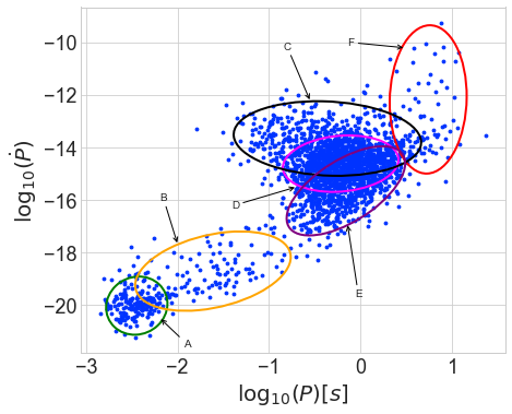
Figure 2: Pulsar P-$\dot{P}$ diagram with Gaussian clusters, obtained after applying XDGMM. The ellipses denote the 95% c.i. contours for the six Gaussian clusters obtained from XDGMM. Clusters A and B describe the millisecond pulsars, whereas the remaining clusters encapsulate the rest of the radio pulsar population. More details about their properties can be found in Table 1.

From the pulsar $P$ and $\dot{P}$, one can estimate a characteristic age ($\tau_{c}$) and the characteristic surface magnetic field ($B_{s}$) after making certain assumptions (Lorimer & Kramer, 2012; Ay et al., 2020):

$$\tau_{c}=\frac{P}{2\dot{P}}$$ (7)

$$B_{s}=\left(\frac{3c^{3}I}{8\pi^{2}R^{6}}\right)^{\frac{1}{2}}\sqrt{P\dot{P}}$$ (8)

where $I$ is the moment of inertia and $R$ is the radius of the neutron stars. Similar to  Ay et al. (2020), we assumed $I=10^{45}\rm{gcm^{2}}$ and $R=10^{6}$ cm. Therefore Eq. 8 simplifies to, $B_{s}=3.2\times 10^{19}\sqrt{P\dot{P}}$ G.

From these equations, we then proceed to calculate the characteristic age and surface magnetic field for each of the cluster populations using the mean ($P$ and $\dot{P}$). The values of $\tau_{c}$ and $B_{s}$ are tabulated in Table 1. These values are mostly in agreement with those in  Ay et al. (2020).

Table 1: The Gaussian cluster parameters obtained after applying XDGMM to the natural log of pulsar $P$ and $\dot{P}$ values. These include the weights, means and covariance matrices of Gaussian clusters A, B, C, D, E and F as indicated in Fig. 2. Characteristic age and characteristic dipole magnetic field strength correspond to the coordinates of the cluster centre and are obtained from Eq. 7 and  8.

Cluster	Weight	Mean ($P$ (sec), $\mathbf{\dot{P})}$	Covariance Matrix	Characteristic Age	Characteristic $B$
				(Yr)	(G)
A	0.0808	(0.003 $0.94\times 10^{-20}$)	$\begin{bmatrix}0.0281&0.0063\\ 0.0063&0.3064\end{bmatrix}$	$6.01\times 10^{9}$	$1.86\times 10^{8}$
B	0.0411	(0.02 $1.94\times 10^{-19}$)	$\begin{bmatrix}0.1809&0.1138\\ 0.1138&0.5701\end{bmatrix}$	$1.98\times 10^{9}$	$2.20\times 10^{9}$
C	0.1923	(0.43 $2.17\times 10^{-14}$)	$\begin{bmatrix}0.2629&-0.0384\\ -0.0384&0.5035\end{bmatrix}$	$3.18\times 10^{5}$	$3.11\times 10^{12}$
D	0.3939	(0.61 $2.39\times 10^{-15}$)	$\begin{bmatrix}0.0999&0.0234\\ 0.0234&0.2889\end{bmatrix}$	$4.02\times 10^{6}$	$1.22\times 10^{12}$
E	0.2750	(0.69 $2.21\times 10^{-16}$)	$\begin{bmatrix}0.1051&0.1698\\ 0.1698&0.7195\end{bmatrix}$	$4.98\times 10^{7}$	$3.96\times 10^{11}$
F	0.0165	(5.51 $6.67\times 10^{-13}$)	$\begin{bmatrix}0.0443&0.0133\\ 0.0133&1.9913\end{bmatrix}$	$1.31\times 10^{5}$	$6.14\times 10^{13}$

3.5 Robustness of XDGMM

Igoshev & Popov (2013) have pointed out that the data classification using GMM does not produce stable results. They showed that the exclusion of magnetars and thermally emitting neutron stars results in different clusters than the ones obtained in  Lee et al. (2012). They also found that upon randomly removing 10% of the data points, the positions of the resulting clusters changes significantly. Hence, they concluded that GMM is oversensitive to small changes in the data, and consequently cannot be used for identifying evolutionary related groups in the pulsar distribution.

To check if our XDGMM-based classification runs into similar problems, we followed the same procedure as in  Igoshev & Popov (2013). We carried out numerical experiments, by randomly removing 10% of the total data points in each trial run, and then applied XDGMM for different number of Gaussian clusters. After repeating this procedure 1000 times with six clusters for classification, we have used $K$-means to find the number of executions which resulted in a figure similar to Fig. 2. We have found that, 69.2% executions resulted in the correct output. We have plotted the 2D histogram of these output clusters as seen in Fig. 3.

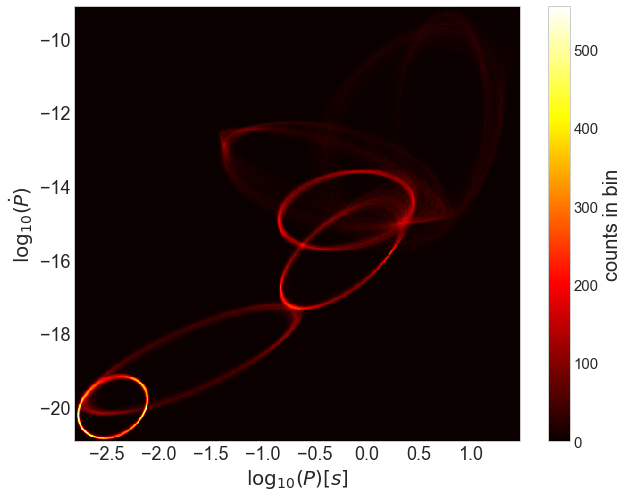
Figure 3: 2-D heatmap of clusters obtained in each of our 1000 numerical experiments obtained by randomly removing 10% of the data points.

From Fig. 3, we find that all the executions result in the same clusters for MSPs, and also the cluster C, D, and E (as seen in Fig. 2). Whereas, there is a clear variation in the cluster corresponding to cluster F in Fig. 2 over multiple executions. Quantitatively, the centroid of this cluster varies by a maximum of 0.5 seconds (in log scale) in x-direction and 0.3 in the y-direction across multiple executions. From this, we can conclude that XDGMM cannot accurately cluster the data when the sample size is low.

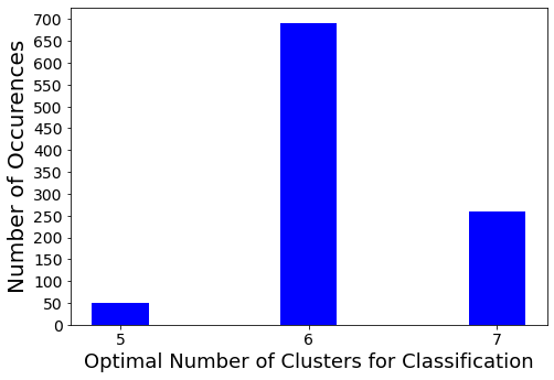
Figure 4: Bar graph of the number of executions resulting in same number of optimal clusters in XDGMM.

We have also found the BIC scores for different number of clusters (ranging from 1-10) for all the 1000 executions. Fig. 4 shows the number of executions which resulted in 5, 6, and 7 as optimal number of clusters. We found that 69.1% executions resulted in six, 26% executions resulted in seven, and 4.9% executions resulted in five as optimal number of clusters. The BIC score for executions resulting in seven clusters was very close (within 100) to the score obtained for six cluster for that particular execution. The case of 4.9% executions resulting in five clusters as optimum could be because of the removal of 10% data was done mainly from a single location.

3.6 GMM for Pulsar Classification

Given that the uncertainties for most pulsars in our dataset are negligibly small, we would like to compare our results with GMM as a cross-check. Therefore, we also applied GMM to the same data described in Sect.3.1 and selected the optimum number of clusters by minimizing BIC in the same way as to be done for XDGMM. We found that by applying BIC (Sec. 3.3) to our data, the optimum number of clusters required to classify this data is six. Hence, assuming that the dataset contains six clusters, we applied GMM to this data set ten times and found that the positions of the resulting clusters is not stable. We get a bimodal distribution for the positions of the clusters, instead of one stable solution. The first case relates to Fig. 5, whereas two clusters are needed to classify the MSPs and the second case relates to Fig. 6, where only one cluster was needed to classify the MSPs. The probability of obtaining one of these two cases was 50%. Therefore, we find that even without randomly removing any pulsars, we do not get a stable solution. Other problems related to application of GMM are pointed out in  Igoshev & Popov (2013).

Figure 5: Result 1 after applying GMM: Two clusters are needed to classify MSPs.

Figure 6: Result 2 after applying GMM: One cluster is obtained to classify MSPs.

Furthermore, even in executions which resulted in the same number of cases, it was sometimes observed that the clusters obtained were not having the same location and axes lengths. As seen in Fig. 7, the position of the clusters corresponding to high energy pulsars varies for different executions.

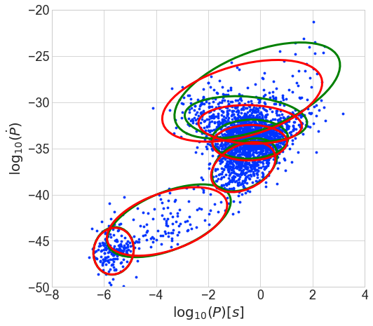
Figure 7: The obtained clusters for different executions of GMM. The red clusters correspond to a single execution and the green clusters correspond to another execution.

The above observations imply that applying GMM on the Pulsar $P$-$\dot{P}$ results in a dichotomy in pulsar classifications with equal probability for the two groups of clusters and even in cases where two clusters were enough to classify MSPs, the position of the clusters corresponding to C, D, and F clusters (from Fig. 2) is varied. Hence, GMM cannot be used for the classification of pulsars in a robust fashion.

4 Conclusions

Two papers within the past decade have classified the radio pulsar population along with other ancillary neutron star datasets, using unsupervised clustering techniques, such as GMM and Dirichlet mixture model (Lee et al., 2012; Ay et al., 2020). We carry out a similar exercise using XDGMM, which is an extension of GMM where the uncertainties in the observed variables are incorporated. Similar to the previous works, we carried out this classification using the logarithm of the period and period derivative. The optimum number of clusters was chosen using the BIC criterion from information theory.

When we apply this method to the latest catalog of radio pulsars, which we obtained from the online ATNF catalog, we find that the optimum number of clusters, which can describe the radio pulsar population is equal to six. Two of these describe the millisecond pulsar population, whereas the remaining radio pulsar population can be grouped into four clusters. However, even within each cluster, there is considerable variation in the types of neutron stars which be found and no cluster can be unambiguously associated with any specific type of pulsar or neutron star. The 95% confidence level ellipses showing the full dataset centered on these clusters can be found in Fig. 2. The mean values, covariance matrices, the characteristic ages and magnetic fields of each of these clusters can be found in Table 1. These results are in accord with the previous works. We also tested the robustness of the XDGMM algorithm using numerical experiments and also point out some advantages compared to the ordinary GMM.

However, we should caution that this statistical classification based on only $P$ and $\dot{P}$ does not offer additional insights into pulsar phenomenology or evolution of the pulsar population, because these likely depends on additional parameters.

To promote transparency in data analysis, we have made available our codes and the data used for this analysis, which can be found at https://github.com/taruntejreddych/XDGMM-for-Pulsar-classification

5 Acknowledgements

We are grateful to the anonymous referee for useful constructive feedback on the manuscript.

References

- Acero et al. (2015) Acero F., et al., 2015, Astrophys. J. Suppl. Ser., 218, 23
- Alford et al. (2008) Alford M. G., Schmitt A., Rajagopal K., Schäfer T., 2008, Reviews of Modern Physics, 80, 1455
- Ay et al. (2020) Ay F., Ince G., Kama\textcommabelowsak M. E., Ek\textcommabelowsi K. Y., 2020, Mon. Not. R. Astron. Soc., 493, 713
- Babu & Feigelson (2006) Babu G. J., Feigelson E. D., 2006, in Gabriel C., Arviset C., Ponz D., Enrique S., eds, Astronomical Society of the Pacific Conference Series Vol. 351, Astronomical Data Analysis Software and Systems XV. p. 127
- Bagchi (2018) Bagchi M., 2018, Universe, 4, 36
- Ball & Brunner (2010) Ball N. M., Brunner R. J., 2010, International Journal of Modern Physics D, 19, 1049
- Bhattacharya & van den Heuvel (1991) Bhattacharya D., van den Heuvel E. P. J., 1991, Physics Reports, 203, 1
- Blandford (1992) Blandford R. D., 1992, Philosophical Transactions of the Royal Society of London Series A, 341, 177
- Bovy et al. (2011) Bovy J., Hogg D. W., Roweis S. T., 2011, Annals of Applied Statistics, 5, 1657
- Cordes & Chatterjee (2019) Cordes J. M., Chatterjee S., 2019, Ann. Rev. Astron. Astrophys. , 57, 417
- Coronado-Blázquez et al. (2019) Coronado-Blázquez J., Sánchez-Conde M. A., Di Mauro M., Aguirre-Santaella A., Ciucă I., Domínguez A., Kawata D., Mirabal N., 2019, JCAP, 2019, 045
- De Luca (2017) De Luca A., 2017, in Journal of Physics Conference Series. p. 012006 (arXiv:1711.07210), doi:10.1088/1742-6596/932/1/012006
- Desai & Kahya (2016) Desai S., Kahya E. O., 2016, Modern Physics Letters A, 31, 1650083
- Fluke & Jacobs (2020) Fluke C. J., Jacobs C., 2020, WIREs Data Mining and Knowledge Discovery, 10, e1349
- Frail et al. (1994) Frail D. A., Weisberg J. M., Cordes J. M., Mathers C., 1994, Astron. J., 436, 144
- Fraix-Burnet et al. (2015) Fraix-Burnet D., Thuillard M., Chattopadhyay A. K., 2015, Frontiers in Astronomy and Space Sciences, 2, 3
- Glushak (2020) Glushak A. P., 2020, Astronomy Reports, 64, 602
- Harding (2013) Harding A. K., 2013, Frontiers of Physics, 8, 679
- Hewish et al. (1968) Hewish A., Bell S. J., Pilkington J. D. H., Scott P. F., Collins R. A., 1968, Nature, 217, 709
- Holoien et al. (2017) Holoien T. W. S., Marshall P. J., Wechsler R. H., 2017, Astron. J., 153, 249
- Igoshev & Popov (2013) Igoshev A. P., Popov S. B., 2013, Mon. Not. R. Astron. Soc., 434, 2229
- Ivezić et al. (2014) Ivezić Ž., Connolly A., Vanderplas J., Gray A., 2014, Statistics, Data Mining and Machine Learning in Astronomy. Princeton University Press
- Kaspi (2010) Kaspi V. M., 2010, Proceedings of the National Academy of Science, 107, 7147
- Keitel (2019) Keitel D., 2019, Mon. Not. R. Astron. Soc., 485, 1665
- Keith et al. (2013) Keith M. J., et al., 2013, Mon. Not. R. Astron. Soc., 429, 2161
- Konar (2017) Konar S., 2017, Journal of Astrophysics and Astronomy, 38, 47
- Koposov et al. (2013) Koposov S. E., Belokurov V., Evans N. W., 2013, Astron. J., 766, 79
- Kramer & Stappers (2015) Kramer M., Stappers B., 2015, in Advancing Astrophysics with the Square Kilometre Array (AASKA14). p. 36 (arXiv:1507.04423)
- Krishnakumar et al. (2021) Krishnakumar M. A., et al., 2021, Astron. & Astrophys., 651, A5
- Kuhn & Feigelson (2017) Kuhn M. A., Feigelson E. D., 2017, arXiv e-prints, p. arXiv:1711.11101
- Kulkarni & Desai (2017) Kulkarni S., Desai S., 2017, Astrophys. and Space Science, 362, 70
- Kulkarni & Desai (2018) Kulkarni S., Desai S., 2018, The Open Journal of Astrophysics, 1, 4
- Lattimer (2012) Lattimer J. M., 2012, Annual Review of Nuclear and Particle Science, 62, 485
- Lee et al. (2012) Lee K. J., Guillemot L., Yue Y. L., Kramer M., Champion D. J., 2012, Mon. Not. R. Astron. Soc., 424, 2832
- Liddle (2007) Liddle A. R., 2007, Mon. Not. R. Astron. Soc., 377, L74
- Lorimer & Kramer (2012) Lorimer D. R., Kramer M., 2012, Handbook of Pulsar Astronomy
- Manchester et al. (2005) Manchester R. N., Hobbs G. B., Teoh A., Hobbs M., 2005, Astron. J., 129, 1993
- McLaughlin et al. (2006) McLaughlin M. A., et al., 2006, Nature, 439, 817
- Melrose et al. (2021) Melrose D. B., Rafat M. Z., Mastrano A., 2021, Mon. Not. R. Astron. Soc., 500, 4549
- Mereghetti (2011) Mereghetti S., 2011, Astrophysics and Space Science Proceedings, 21, 345
- Meszaros (1992) Meszaros P., 1992, High-energy radiation from magnetized neutron stars
- Pathak & Bagchi (2018) Pathak D., Bagchi M., 2018, Astron. J., 868, 123
- Roche (2011) Roche A., 2011, arXiv e-prints, p. arXiv:1105.1476
- Schwarz (1978) Schwarz G., 1978, Annals of Statistics, 6, 461
- Shklovskii (1970) Shklovskii I. S., 1970, Soviet Astronomy, 13, 562
- Stairs (2003) Stairs I. H., 2003, Living Reviews in Relativity, 6, 5
- Stairs (2004) Stairs I. H., 2004, Science, 304, 547
- Taylor (1994) Taylor Jr. J. H., 1994, Reviews of Modern Physics, 66, 711
- Vivekanand & Narayan (1981) Vivekanand M., Narayan R., 1981, Journal of Astrophysics and Astronomy, 2, 315
- Vranešević & Melrose (2011) Vranešević N., Melrose D. B., 2011, Mon. Not. R. Astron. Soc., 410, 2363
- Wolszczan & Frail (1992) Wolszczan A., Frail D. A., 1992, Nature, 355, 145
- Woods & Thompson (2006) Woods P. M., Thompson C., 2006, Soft gamma repeaters and anomalous X-ray pulsars: magnetar candidates. pp 547–586