FROM STARSPOTS TO STELLAR CORONAL MASS EJECTIONS
– REVISITING EMPIRICAL STELLAR RELATIONS –

Abstract

Upcoming missions, including the James Webb Space Telescope, will soon characterize the atmospheres of terrestrial-type exoplanets in habitable zones around cool K- and M-type stars searching for atmospheric biosignatures. Recent observations suggest that the ionizing radiation and particle environment from active cool planet hosts may be detrimental for exoplanetary habitability. Since no direct information on the radiation field is available, empirical relations between signatures of stellar activity, including the sizes and magnetic fields of starspots, are often used. Here, we revisit the empirical relation between the starspot size and the effective stellar temperature and evaluate its impact on estimates of stellar flare energies, coronal mass ejections, and fluxes of the associated stellar energetic particle events.

1 Introduction

The increasing sensitivity of ground and space-based instruments has led to an exponential growth in the detection and characterization of stellar flares. Space missions such as Kepler (e.g., Koch et al., 2010), Gaia (e.g., Prusti et al., 2016) and TESS (Ricker et al., 2015) have contributed significantly to our understanding of the statistical properties of energies and frequencies of flares and the underlying mechanisms generating them. These new statistical studies of stellar flares complemented with multi-wavelength observations of eruptive events opened a new window to search for signatures of flare associated Coronal Mass Ejections (CMEs) and stellar energetic particle (SEP) events and their impact on exoplanetary environments (e.g., Airapetian et al., 2016, 2020; Atri, 2019; Herbst et al., 2019; Scheucher et al., 2020). Some of the most important properties of flares, CMEs, and SEPs, including their energies and frequency of occurrence, are determined by the strength of the magnetic field and the size of the stellar active region associated with the starspot area derived from observations. Thereby, the amplitude of the rotationally modulated brightness variation and the effective (photospheric) stellar temperature are directly derived from observations. In contrast, the evaluation of the starspot temperatures (e.g. Notsu et al., 2013) is based on the empirical scaling with the effective temperature of the star derived by Berdyugina (2005). Although this relation often is applied to derive the starspot areas of G-, K-, and M-dwarfs (Morris et al., 2018; Notsu et al., 2019; Howard et al., 2020a; Yamashiki et al., 2019), more accurate observations and stellar targets are required for the validation and revision of the current empirical equation.

In this paper, we first reanalyze the sample by Berdyugina (2005) using the scipy.optimize.leastsq fitting routine. Thereby, the Jacobian matrix is multiplied with the residual variances, estimated by the mean square errors. The resulting covariance matrix is then used to derive the standard error and, therefore, the $\pm\sigma$ uncertainty. Further, we obtain a revised empirical relation, quantifying for the first time an error band.

Additionally, we expand the data set utilizing data from Biazzo et al. (2006) and Valio (2017) to derive an updated empirical relation and investigate its impact on empirical estimates of the fundamental properties of stellar flares and CMEs.

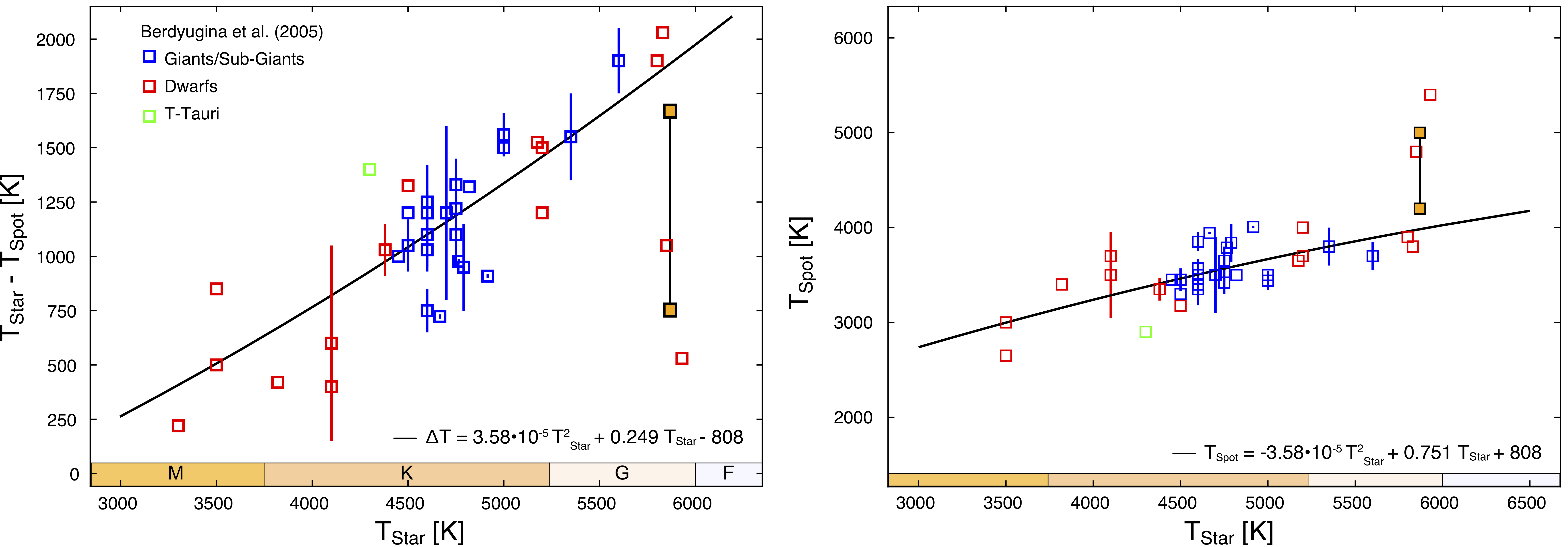
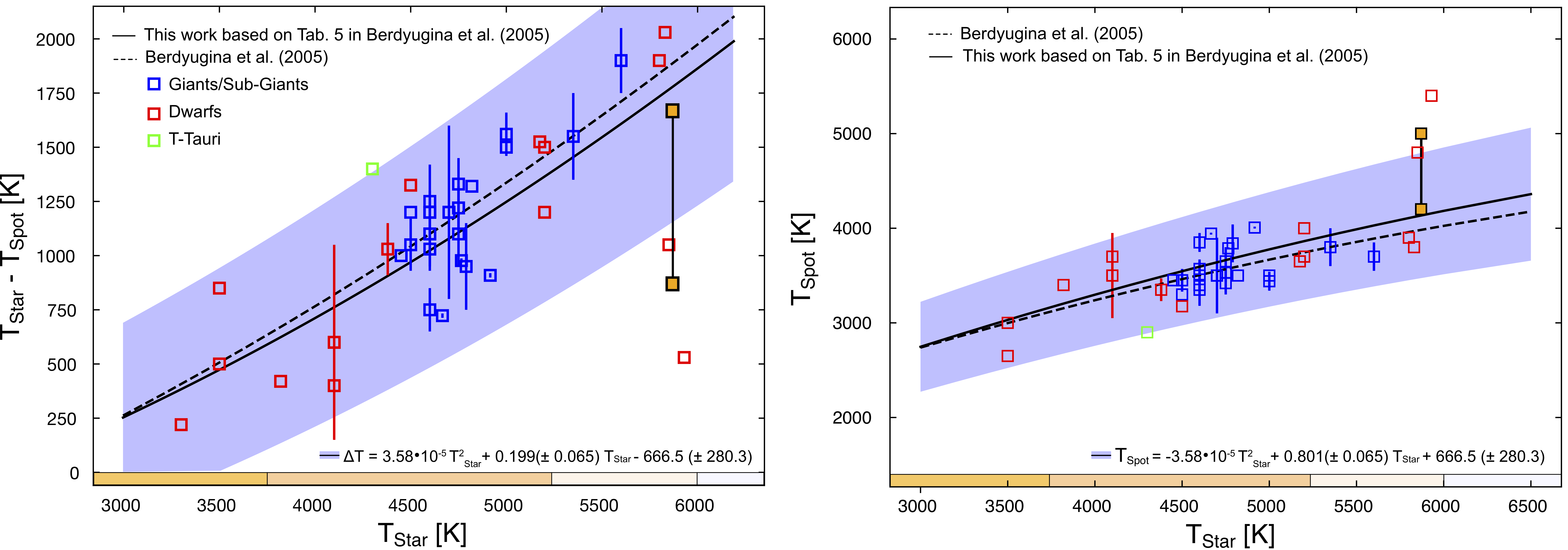
Figure 1: Upper left: Difference between stellar photosphere and spot temperatures for dwarf stars (red squares), active giants/sub-giants (blue squares), and a T-Tauri star (green square). Figure based on the data given in Table 5 of Berdyugina (2005). Upper right: Starspot temperature as function of the stellar (photospheric) temperature. Here the the orange squares give typical solar umbra (lower symbol, $T_{\mathrm{Spot}}\approx$ 4100 K) and penumbra (upper symbol, $T_{\mathrm{Spot}}\approx$ 5000 K) temperatures. Lower left: Re-analysis of the sample discussed in Berdyugina (2005) based on the mathematical approach disscued in the text. Lower right: Corresponding $T_{\mathrm{Star}}$-$T_{\mathrm{Spot}}$-relation.

2 The Empirical Relation Between Stellar and Starspot Temperatures

The empirical relation derived by Berdyugina (2005) is a second-order polynomial fit to the data representing the starspot temperature contrast with respect to the effective temperatures of cool dwarfs and giant stars. While the effective stellar temperatures are derived with high precision, the temperatures of starspots are obtained from various observational techniques including Doppler imaging, light curve modeling, and molecular bands and atomic line-depth ratios (see the extended discussion in Berdyugina, 2005). The spot temperature recovered from molecular band modeling uses the combining spectra of suitable standard stars of different effective temperatures weighted by a spot filling factor and continuum surface flux derived from radiative transfer models (Kurucz, 1991) provides the continuum surface flux ratio between the spot and the quiet (unmagnetized) photosphere. Also, molecular band modeling is sensitive to the assumed photospheric temperature, chemical composition, and Doppler shifts across the spots, which may affect the spot filling factor (Berdyugina, 2002; O’Neal et al., 2004). However, strong magnetic fields affect the optical thickness of molecular bands via modified vertical temperature gradients introduced by vertical motions (Evershed effect), which is not accounted for in ”non-magnetic” radiative transfer models.

The stellar sample by Berdyugina (2005) utilizing the Doppler Imaging method includes 17 G-K (super)giants, eight main-sequence stars (two G-types and four K- and M-types each), and one pre-main-sequence star. Interestingly, the young G-type EK Dra, has a much lower temperature contrast than other young G-type stars and the current Sun’s umbra. This may be the result of the non-uniqueness of the temperature reconstruction and the possible importance of the vertical energy transport within starspots which needs to be considered in the multi-dimensional magnetohydrodynamic modeling of magnetoconvection.

As shown in the upper left panel of Fig. 1, Berdyugina (2005) found that the relation between the effective stellar temperature ($T_{\mathrm{Star}}$) and the starspot temperature ($T_{\mathrm{Spot}}$) for the cool star regime is best described as

$$\Delta T(T_{\mathrm{Star}})= T_{\mathrm{Star}}-T_{\mathrm{Spot}}$$

$$= 3.58\cdot 10^{-5}~{}T_{\mathrm{Star}}^{2}+0.249~{}T_{\mathrm{Star}}-808.$$ (1)

As can be seen, $\Delta T(T_{\mathrm{Star}})$ increases with increasing stellar temperature, varying between about 200 K for cool M-stars (M4) up to about 2000 K for G-type stars (G0), which leads to a clear tendency towards higher-contrast spots -with respect to the photosphere- in hotter stars. In addition, almost no difference can be found between active dwarfs and giants in the K- and G-star regime. The latter, according to Berdyugina (2005), implies that the nature of starspots most likely is the same in all active stars.

Taking into account that $\Delta T(T_{\mathrm{Star}})=T_{\mathrm{Star}}-T_{\mathrm{Spot}}$ the temperature of starspots can rather easily be derived once the effective stellar temperature is known. Based on Eq. (1) the starspot temperature is given by

$$T_{\mathrm{Spot}}=-3.58\cdot 10^{-5}~{}T_{\mathrm{Star}}^{2}+0.751~{}T_{\mathrm{Star}}+808.$$ (2)

$T_{\mathrm{Spot}}$ as a function of the effective stellar temperature is displayed in the upper right panel of Fig. 1.

As can be seen, starspot temperatures may vary between about 2900 K in the case of M-dwarfs up to above 4000 K on G-type stars. A direct comparison to the known sunspot (umbra)-temperature variations (filled orange squares) of about 4100 K in umbra regions and 5000 K in penumbra regions shows that the widely used relation by Berdyugina (2005) is not able to reflect the solar values. Thus, although the relation, in principle, should be applicable for all stellar types, and therefore has been widely used in the stellar and exoplanetary community (see, e.g., Notsu et al., 2013; Maehara et al., 2017), it should be treated with caution, in particular in studies of young G-type stars (most recently, e.g., Notsu et al., 2019; Namekata et al., 2019; Howard et al., 2020a).

2.1 Re-analysis of the sample by Berdyugina (2005)

Figure 5 of Berdyugina (2005) presents no error estimates for the relation between the effective stellar temperature and the temperature of the starspot, thus, for the first time, our approach allows us to estimate an error band. We find the relation between the effective stellar and the starspot temperature to be best described by:

$$\begin{split}\Delta T(T_{\mathrm{Star}})=~{}&3.58\cdot 10^{-5}~{}T_{\mathrm{Star}}^{2}+0.199(\pm 0.065)~{}T_{\mathrm{Star}}\\ &-666.5(\pm 280.3),\end{split}$$ (3)

as shown in the lower left panel of Fig. 1. In addition, the corresponding relation between stellar temperature and starspot temperature then is given by:

$$\begin{split}T_{\mathrm{Spot}}=~{}&-3.58\cdot 10^{-5}~{}T_{\mathrm{Star}}^{2}+0.801(\pm 0.065)~{}T_{\mathrm{Star}}\\ &+666.5(\pm 280.3)\end{split}$$ (4)

as shown in the lower right panel of Fig. 1. Both panels show a direct comparison between the stellar sample (colored symbols), the relations by Berdyugina (2005) (Eqs. (1) and (2), dashed lines), and the newly-derived relations given by Eqs. (3) and (4), displayed as solid lines with corresponding blue error band.

As can be seen, Eq. (1) is well within the error band of our newly-derived relation. However, although being in good agreement in the cool M-star regime Eqs. (1) and (3) differ by up to 169$\pm$683 K in the case of G-type stars. Nevertheless, the newly-derived relationships, including their $\pm\sigma$ uncertainties, are in good agreement with the stellar sample discussed in Berdyugina (2005). In particular, Eq. (4) suggests that in the case of Sun-like stars (with $T_{\mathrm{Star}}$ = 5780 K) starspot temperatures of $4100\pm 656$ K can be expected. This is also in good agreement with the range of the measured solar umbra/penumbra temperatures.

2.2 Extending the stellar sample by Berdyugina (2005)

Table 1: Comparison of former (second column) and newly-derived values of $T_{\mathrm{Spot}}$ based on Eq. 4 (third column) and Eq. 5 (fourth column). The former derived values are based on Berdyugina (2005) (see Eq. (2)).

$T_{\mathrm{eff}}$ [K]	$T_{\mathrm{Spot}}$ [K]	$T_{\mathrm{Spot}}\pm\Delta T_{\mathrm{Spot}}$ [K]	$T_{\mathrm{Spot}}\pm\Delta T_{\mathrm{Spot}}$ [K]
3000	2739	2747 $\pm$ 475	2495 $\pm$ 498
3200	2845	2863 $\pm$ 488	2654 $\pm$ 510
3400	2948	2976 $\pm$ 501	2811 $\pm$ 523
3600	3048	3086 $\pm$ 514	2964 $\pm$ 535
3800	3145	3193 $\pm$ 527	3115 $\pm$ 547
4000	3239	3297 $\pm$ 540	3263 $\pm$ 559
4200	3331	3399 $\pm$ 553	3408 $\pm$ 571
4400	3419	3498 $\pm$ 566	3550 $\pm$ 583
4600	3505	3594 $\pm$ 579	3690 $\pm$ 595
4800	3588	3686 $\pm$ 592	3826 $\pm$ 607
5000	3668	3777 $\pm$ 605	3960 $\pm$ 619
5200	3745	3864 $\pm$ 618	4090 $\pm$ 631
5400	3819	3948 $\pm$ 631	4218 $\pm$ 643
5600	3891	4029 $\pm$ 644	4343 $\pm$ 655
5800	3959	4108 $\pm$ 657	4465 $\pm$ 667
6000	4025	4184 $\pm$ 670	4585 $\pm$ 679
6200	4088	4257 $\pm$ 683	4701 $\pm$ 691

By now two more samples have been published in the literature:

1. Biazzo et al. (2006), who investigated the observations of three K-type stars IM Peg (K2), HK Lac (K0), and VY Ari (K3-4) and the three G-type stars $\lambda$ And (G8), $\kappa$1 Cet (G5), and HD 206860

2. Valio (2017), who modeled the G-type stars CoRoT-2 (G7), CoRoT-18 (G9), Kepler-17 (G2), and Kepler-63 (G8), the F-type stars CoRoT-4 (F8), CoRoT-5 (F9), and CoRoT-6 (F9) as well as the K-star CoRoT-8 (K1) based on a planetary transit model.

Both samples have been derived by methods other than the Doppler Imaging: while Biazzo et al. (2006) based their analysis on photospheric line-depth ratios and utilized the simplified spot model by Frasca et al. (2005), Valio (2017) used an exoplanet transit model to investigate the stellar relation between $T_{\rm{Spot}}$ and $T_{\rm{Star}}$. The spatial resolution of both the Doppler Imaging and the transit method is poor. In contrast, no information on both the spatial resolution and the filling factors the starspots have in active regions is available utilizing the method discussed in Biazzo et al. (2006). Consequently, in all three cases, the resulting spot contrasts should only be seen as typical averaged values that might be underestimated. Thus, further observations, for example, using instruments like the XMM-Newton and NICER, as well as numerical modeling of starspot temperatures of cool dwarfs allowing for an extended empirical characterization, are required.

A comparison of both samples to the relation between stellar and starspot temperatures based on Eqs. (2) and (4) is given in the upper panel of Fig. 2. It shows that the relation by Berdyugina (2005) given as a dashed line is not able to reflect the starspot temperatures of both Biazzo et al. (2006) and Valio (2017), which strengthens the argument that the function needs to be treated with caution when G-type stars are investigated. However, our newly-derived function (Eq. (4), solid black line), and its error band is in relatively good agreement with the new sample. Please note that in addition the linear fit provided by Valio (2017) is provided (blue dashed line) which is best represented as $T_{\mathrm{Spot}}=0.667\cdot T_{\mathrm{Star}}+979.4$, which well describes the new sample, however, can not characterize the stellar sample by Berdyugina (2005).

Assuming the nature of starspots to be the same in all active stars a more reliable correlation that is able to describe the data of all three samples is needed. Therefore, in a second step, we:

1. extended the sample used by Berdyugina (2005) by including the data from Biazzo et al. (2006) and Valio (2017),

2. utilized the same approach discussed in Sec. 2.1 to derive a more universal relations for both $T_{\mathrm{Spot}}$ and $\Delta T(T_{\mathrm{Star}})$.

Based on the samples by Berdyugina (2005), Biazzo et al. (2006), and Valio (2017) we find $T_{\mathrm{Spot}}$ to be represented best as

$$\begin{split}T_{\mathrm{Spot}}=~{}&-3.58\cdot 10^{-5}~{}T_{\mathrm{Star}}^{2}+1.0188(\pm 0.068)~{}T_{\mathrm{Star}}\\ &+239.3(\pm 317.8).\end{split}$$ (5)

A comparison between the sample (colored symbols), the originally derived function by Berdyugina (2005) (dashed line) and Eq. (5) is shown in the middle panel of Fig. 2 and the third column of Table 1. As can be seen, Eq. (5) represents the entire stellar sample, including, for the first time, the well-known solar sunspot temperature variations.

The lower panel of Fig. 2 shows the results for the difference between stellar and starspot temperature which according to Eqs.(1) and (5) is given by:

$$\begin{split}\Delta T(T_{\mathrm{Star}})=~{}&3.58\cdot 10^{-5}~{}T_{\mathrm{Star}}^{2}-0.0188(\pm 0.068)~{}T_{\mathrm{Star}}\\ &-239.3(\pm 317.8).\end{split}$$ (6)

As can be seen, $\Delta T(T_{\mathrm{Star}})$ still increases with increasing stellar temperature, as indicated by Berdyugina (2005), however, is less steep than previously suggested. In the mean $\Delta T(T_{\mathrm{Star}})$ varies between about 500 K for cool M-stars (M4) up to about 1500 K for G-type stars (G0). Consequently, the higher-contrast of spots with respect to the photosphere of hotter stars is not necessarily as pronounced as previously thought.

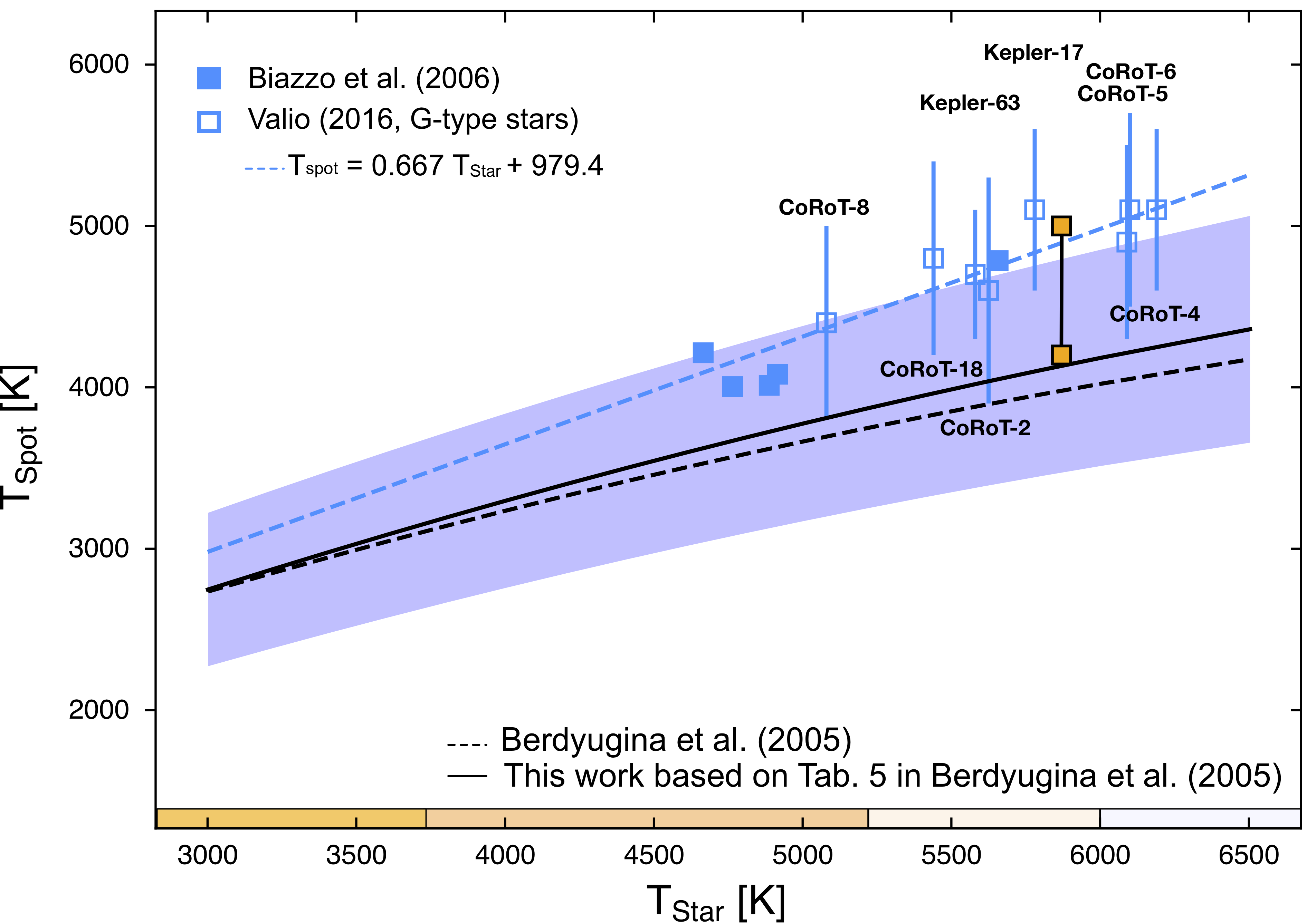
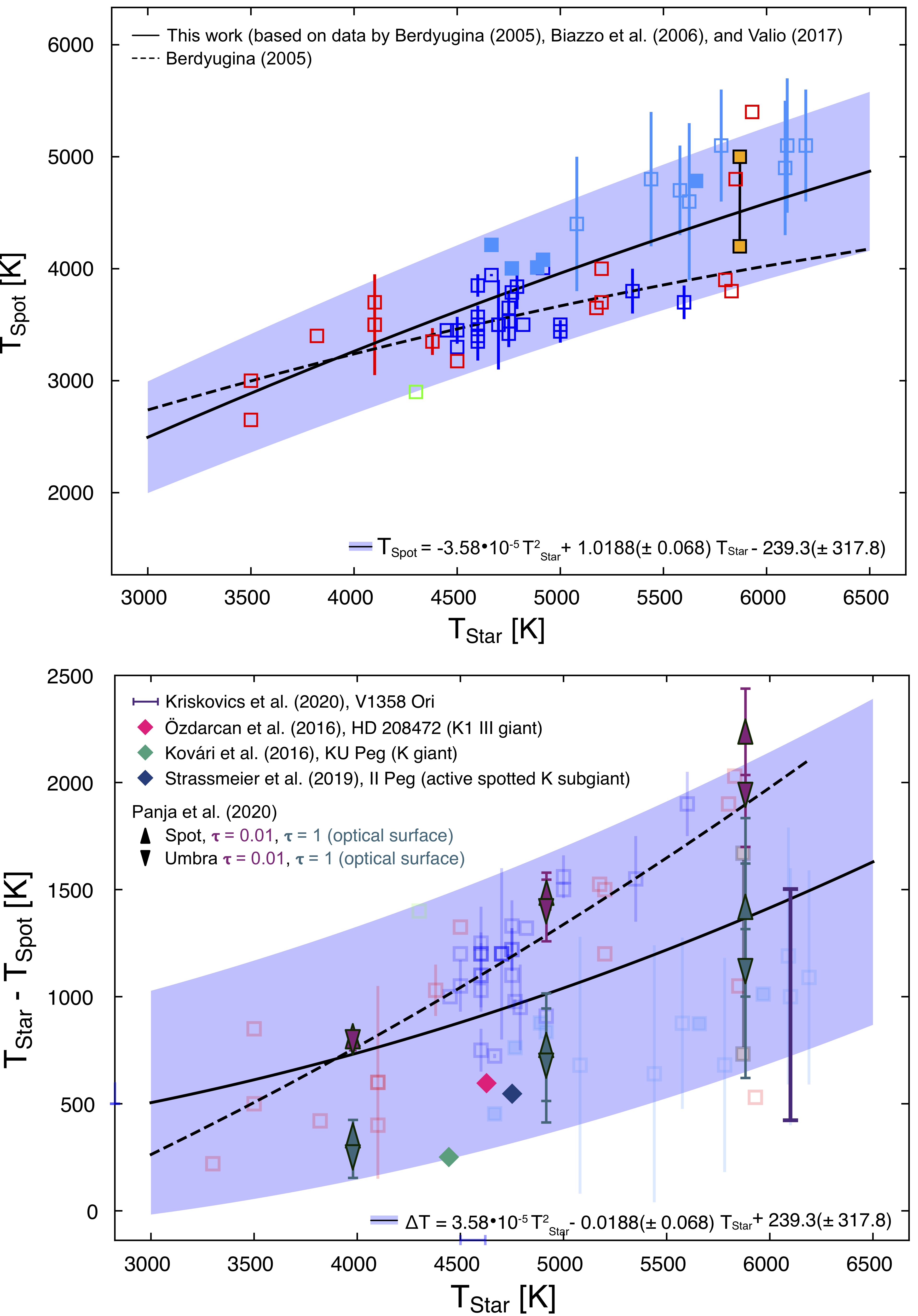
Figure 2: Upper panel: Comparison of Eq. (4) to the sample by Biazzo et al. (2006) and Valio (2017). Middle panel: Newly-derived $T_{\mathrm{Star}}$-$T_{\mathrm{Spot}}$-relation based on the entire sample. Lower panel: Corresponding newly-derived $T_{\mathrm{Star}}$-$\Delta T(T_{\mathrm{Star}})$-relation.

In order to test the validity of Eq. (6) a comparison with the most recent measurements and simulations is performed. Shown are the results of the Doppler Imaging of V1358 Ori, a young G9-type star (purple line Kriskovics et al., 2019), the K-giants HD208472 (magenta diamond Özdarcan et al., 2016) and KU Peg (green diamond Kővári et al., 2016), the active K subgiant II Peg (blue diamond Strassmeier et al., 2019), and the new 3D MHD model results by Panja et al. (2020) (colored triangles). As can be seen, both the observations and the simulations are remarkably well-described by our newly-derived relation. In addition, the results by Panja et al. (2020) suggest a systematically lower contrast of about 300-400 K compared to that derived by Berdyugina (2005).

More importantly, $\Delta T(T_{\mathrm{Star}})$ is often used as a semi-empirical quantity to derive other stellar relations like, for example, to estimate starspot areas (see, e.g., Notsu et al., 2013; Shibata et al., 2013; Notsu et al., 2019), stellar flare energies (see, e.g., Notsu et al., 2019; Howard et al., 2020a), and the properties of stellar Coronal Mass Ejections (CMEs, see, e.g., Takahashi et al., 2016). Thus, the newly-derived functions discussed here have a direct impact on previously published results and the semi-empirical relations based upon these functions.

Table 2: Derived starspot temperatures $T_{\mathrm{Spot}}$, starspot areas normalized to the area of the star $A_{\mathrm{Spot}}/A_{\mathrm{Star}}$ for selected stellar Kepler observations of M-, K, and G-type stars published in McQuillan et al. (2014). The calculated values based on the relations published by Berdyugina (2005) are given in columns 4 and 6, respectively. The results based on the newly-derived relations (Eqs. (5), and (6)) are given in columns 5 and 7. (This table is available in its entirety in a machine-readable form in the online journal. A portion is shown here for guidance regarding its form and content.)

KIC ID	$T_{\mathrm{Star}}$ [K]	$\Delta F/F$	$T_{\mathrm{Spot}}$ [K]	$T_{\mathrm{Spot}}\pm\Delta$ [K]	$A_{\mathrm{Spot}/A_{\mathrm{Star}}}$	$A_{\mathrm{Spot}/A_{\mathrm{Star}}}\pm\Delta$
6060042	3300	0.011	2896	2733 $\pm$ 542	0.027	0.020$\begin{subarray}{c}+0.340\\ -0.007\end{subarray}$
10067340	3400	0.023	2948	2811 $\pm$ 549	0.052	0.042$\begin{subarray}{c}+0.446\\ -0.014\end{subarray}$
5193112	3500	0.009	2998	2888 $\pm$ 556	0.019	0.016$\begin{subarray}{c}+0.122\\ -0.005\end{subarray}$
8183277	3600	0.006	3048	2964 $\pm$ 563	0.012	0.010$\begin{subarray}{c}+0.061\\ -0.003\end{subarray}$
5428199	3700	0.002	3097	3040 $\pm$ 570	0.004	0.004$\begin{subarray}{c}+0.020\\ -0.001\end{subarray}$
2832398	3800	0.017	3145	3115 $\pm$ 576	0.032	0.031$\begin{subarray}{c}+0.124\\ -0.010\end{subarray}$
6584163	3900	0.006	3192	3190 $\pm$ 583	0.010	0.011$\begin{subarray}{c}+0.036\\ -0.003\end{subarray}$
3974567	4000	0.012	3239	3263 $\pm$ 590	0.020	0.021$\begin{subarray}{c}+0.062\\ -0.006\end{subarray}$
5513890	4100	0.005	3285	3336 $\pm$ 597	0.008	0.008$\begin{subarray}{c}+0.022\\ -0.002\end{subarray}$
3954449	4200	0.012	3331	3408 $\pm$ 604	0.021	0.022$\begin{subarray}{c}+0.053\\ -0.007\end{subarray}$
4764328	4300	0.006	3375	3480 $\pm$ 610	0.009	0.010$\begin{subarray}{c}+0.021\\ -0.003\end{subarray}$
6225454	4400	0.011	3419	3550 $\pm$ 617	0.018	0.020$\begin{subarray}{c}+0.038\\ -0.006\end{subarray}$
7867109	4500	0.006	3463	3620 $\pm$ 624	0.009	0.011$\begin{subarray}{c}+0.019\\ -0.003\end{subarray}$
3337674	4600	0.050	3505	3690 $\pm$ 630	0.075	0.085$\begin{subarray}{c}+0.140\\ -0.023\end{subarray}$
4842623	4700	0.012	3547	3758 $\pm$ 638	0.018	0.021$\begin{subarray}{c}+0.032\\ -0.006\end{subarray}$
2711354	4800	0.006	3588	3826 $\pm$ 644	0.009	0.011$\begin{subarray}{c}+0.015\\ -0.003\end{subarray}$
3763109	4900	0.004	3628	3893 $\pm$ 651	0.006	0.007$\begin{subarray}{c}+0.009\\ -0.002\end{subarray}$
3834448	5000	0.003	3668	3960 $\pm$ 658	0.004	0.004$\begin{subarray}{c}+0.005\\ -0.001\end{subarray}$
3097429	5100	0.015	3707	4025 $\pm$ 665	0.021	0.025$\begin{subarray}{c}+0.029\\ -0.006\end{subarray}$
2993430	5200	0.005	3745	4090 $\pm$ 672	0.007	0.008$\begin{subarray}{c}+0.009\\ -0.002\end{subarray}$
3628249	5300	0.002	3783	4155 $\pm$ 678	0.003	0.004$\begin{subarray}{c}+0.004\\ -0.001\end{subarray}$
4077780	5400	0.016	3819	4218 $\pm$ 685	0.022	0.026$\begin{subarray}{c}+0.025\\ -0.006\end{subarray}$
4276419	5500	0.015	3856	4281 $\pm$ 692	0.020	0.024$\begin{subarray}{c}+0.021\\ -0.005\end{subarray}$
5531826	5600	0.010	3891	4343 $\pm$ 699	0.013	0.016$\begin{subarray}{c}+0.014\\ -0.004\end{subarray}$
5898935	5700	0.021	3926	4405 $\pm$ 705	0.027	0.033$\begin{subarray}{c}+0.027\\ -0.007\end{subarray}$
4069078	5800	0.009	3959	4465 $\pm$ 713	0.011	0.013$\begin{subarray}{c}+0.010\\ -0.003\end{subarray}$
3343950	5900	0.005	3993	4525 $\pm$ 719	0.007	0.008$\begin{subarray}{c}+0.006\\ -0.002\end{subarray}$
3547642	6000	0.002	4025	4585 $\pm$ 726	0.002	0.002$\begin{subarray}{c}+0.002\\ -0.001\end{subarray}$
5282952	6100	0.001	4057	4643 $\pm$ 733	0.002	0.002$\begin{subarray}{c}+0.001\\ -0.001\end{subarray}$
1570150	6200	0.011	4088	4701 $\pm$ 740	0.014	0.017$\begin{subarray}{c}+0.011\\ -0.003\end{subarray}$
5196646	6300	0.001	4118	4758 $\pm$ 746	0.001	0.001$\begin{subarray}{c}+0.001\\ -0.001\end{subarray}$
7116137	6400	0.002	4148	4815 $\pm$ 753	0.003	0.003$\begin{subarray}{c}+0.002\\ -0.001\end{subarray}$

3 From Starspot Temperatures to the Estimation of the Starspot Size

According to Maehara et al. (2012), Shibata et al. (2013), and Notsu et al. (2013, 2019) the stellar area covered by a starspot ($A_{\mathrm{Spot}}$) normalized by the projected stellar hemispherical area $A_{\mathrm{Star}}=\pi\cdot R_{\mathrm{Star}}^{2}$ can be described as

$$\frac{A_{\mathrm{Spot}}}{A_{\mathrm{Star}}}=\left[1-\left(\frac{T_{\mathrm{Spot}}}{T_{\mathrm{Star}}}\right)^{4}\right]^{-1}\frac{\Delta F}{F},$$ (7)

where $\Delta F/F$ is the stellar brightness variation normalized by the average stellar brightness measured by, for example, the Kepler instrument (see, e.g., Shibayama et al., 2013; McQuillan et al., 2014), the TESS instrument (see, e.g., Stassun et al., 2019), or the Evryscope instrument (see Howard et al., 2019, 2020a).

To investigate the impact of the newly-derived starspot-temperature-relation given in Eq. (5), Table 2, amongst others, shows the derived $A_{\rm{Spot}}/A_{\rm{Star}}$ values of selected Kepler main-sequence stars published in McQuillan et al. (2014) with stellar temperatures between 3300 K (mid M-stars) and 6400 K (late G-stars). Additionally, the stellar brightness variation normalized by the average stellar brightness ($\Delta F/F$) and the starspot temperatures derived based on Eq. (2) (fourth column) and Eq. (5) (fifth column) are listed.

It shows that the derived starspot temperatures differ on average by 160 K in the case of M-stars and up to 660 K in G-type stars. More importantly, utilizing the whole stellar sample by McQuillan et al. (2014), the average difference of the derived $A_{\rm{Spot}}/A_{\rm{Star}}$-values based on the former relations by Berdyugina (2005) and the newly-derived relation discussed in this study is in the order of 20% in the case of G-type stars while being up to 40% in the case of M-type stars, implying that previous studies most likely underestimated the sizes of, in particular, starspots on M-stars.

Assuming the existence of a few large starspot groups on the stellar surface and starspot lifetimes exceeding the rotational period of the star (Maehara et al., 2017), based on Eqs. (1), (5) and (7) the area of the starspots normalized to the area of the solar hemisphere ($A_{\odot}$) further can be expressed as

$$A_{\mathrm{Spot}}=\left(\frac{R_{\mathrm{Star}}}{R_{\odot}}\right)^{2}\frac{T_{\mathrm{Star}}^{4}}{T_{\mathrm{Star}}^{4}-\left[T_{\mathrm{Star}}-\Delta T(T_{\mathrm{Star}})\right]^{4}}\frac{\Delta F}{F_{\mathrm{Star}}}.$$ (8)

A comparison of the solar spot group areas (black dots, Sammis et al., 2000) and the 30-min cadence sample of Sun-like stars ($T_{\rm{Star}}$=5100 - 6000 K) by Notsu et al. (2019)(blue crosses) is displayed in the upper panel of Fig. 3. As already discussed in Notsu et al. (2019), the majority of the detected superflares seem to occur on Sun-like stars with large starspots (see discussion in Notsu et al., 2019). In comparison, the values based on the newly derived relations are shown in the middle panel of Fig. 3. Note that the original sample by Notsu et al. (2019) has further been updated by utilizing the stellar temperatures and stellar radii given by the Gaia-DR2 catalog (Berger et al., 2018). Although the derived stellar spot group areas are in fairly good agreement, our approach, for the first time, gives an error estimate depending on the characteristics of each star. As in the case of the $A_{\rm{Spot}}/A_{\rm{Star}}$ values derived from the sample by McQuillan et al. (2014), our newly-derived $A_{\rm{Spot}}/A_{\rm{Sun}}$ values based on the updated sample by Notsu et al. (2019) indicate a previous underestimation of the starspot sizes of Sun-like stars.

As discussed, the latter, however, has a more substantial impact on the K- and M-star regime. Based on the Evryscope light curve measurements of 113 cool stars with intense stellar flares (Howard et al., 2019, 2020a) new spot group areas have been derived. The results are shown in the lower panel of Fig. 3. As can be seen, the newly-derived upper limits result in group areas which are up to one order of magnitude higher than the previously derived values (see Howard et al., 2020a, Table 1), which has further implications on the interpretation of the corresponding flare energies possibly released from these starspots.

4 FROM Starspot Sizes To Stellar Flare energies

Stellar flares are sudden releases of magnetic energy that is stored in magnetic active regions. According to Sturrock et al. (1984), Shibata et al. (2013) and Notsu et al. (2019), the upper limit of the total released flare energy $E_{\text{flare }}$ can be described as constant fraction of the total non-potential (stressed) magnetic field energy of the active region (see Emslie et al., 2012), and thus as a rather simple scaling-law in the form of

$$E_{\text{flare }} \approx fE_{\text{mag }}$$ (9)

$$\approx f\frac{B^{2}}{8\pi}A_{\text{spot }}^{3/2}$$

and thus

$$E_{\text{flare }} \approx a\left(\frac{f}{0.1}\right)\left(\frac{B}{10^{3}~{}\rm{G}}\right)^{2}\left(\frac{A_{\text{Spot }}/(2\pi R_{\odot}^{2})}{0.001}\right)^{3/2},$$ (10)

where $a$ = 7 $\times$ 10³² erg, $f$ gives the fraction of magnetic energy released as flare energy, and $B$ represents the magnetic field strength of the solar/stellar active region (AR) given in Gauss. It becomes apparent that the derived spot temperature is a critical parameter for determining the flare energy plotted in the panels of Figs. 3 and 4. Thereby, $f$ often is assumed to be in the order of 10%, with upper limits reaching 50% (see Schrijver et al., 2012) or even higher (see Aschwanden et al., 2014).

In addition, many years of research on our host star have shown that ARs producing intense flares tend to have a larger spot area as well as morphological and magnetic complexity. Large amounts of magnetic energy are accumulated in ARs; hence, it is reasonable to be larger in the spot area. At the same time, the morphological and magnetic complexity of an AR is manifested during its evolution and serves as a trigger of eventual flare eruption (for a comprehensive review see Toriumi & Wang, 2019). Further, a multi-wavelength multi-observatory Sun-as-a-star study on the spectral irradiance observations of transiting ARs has been performed by Toriumi et al. (2020). Since the complexity and wealth of observational evidence concerning ARs can not be captured, Eqs. (9) and (10) can only be considered as simple but yet valuable approximations that provide a baseline for the construction of empirical relations of stellar ARs and flares. Several studies (e.g. Basri & Nguyen, 2018) emphasize that it is not clear whether the brightness modulation amplitude is related to the size of superflare-generating starspots. However, most recently, Namekata et al. (2020) showed that the area estimated from the rotational modulation is consistent with the maximum in-transit spots, indicating that the Kepler light-curve amplitude is a good indicator of the maximum visible spot size, and thus is a good proxy for the energy released in a flare.

Thus, keeping in mind that the contours reflect the maximum energy release limit, Eq.(10) can be used to study the influence of the magnetic field strength of starspots on the energy released in a flare. The first two panels of Fig. 3 show the corresponding contours for B-values of 3000 G, 2000 G, 1000 G, and 500 G, respectively. As can be seen in the upper panel of Fig. 3, the majority of the solar observations (black dots, from Sammis et al., 2000) can be found below the $B_{\rm{Spot}}$ = 500 G contour line when $f=$ 0.1 is assumed. Note, however, that according to Aulanier et al. (2013), these contour lines only account for the outer spot area. Correspondingly, the represented B-values have to be multiplied by a factor of five to reflect the magnetic field strength of the spot itself. With that, the solar observations point to an upper limit of $B_{\rm{Spot}}$ = 2500 G, which is in good agreement with observations that show $B_{\rm{Spot}}$ to vary between 1500 G and 3600 G (Livingston & Watson, 2015). However, a small number of observations indicate the existence of higher $B_{\rm{Spot}}$-values, which might be a direct indicator that the solar dynamo is capable of causing a higher maximum energy release limit. The latter further puts emphasis on the existence of strong solar events as detected in the cosmogenic radionuclide records of ¹⁰Be, ¹⁴C, and ³⁶Cl around AD774/775, AD 993/994, and BC660 (Miyake et al., 2012; Mekhaldi et al., 2015; O’Hare et al., 2019, respectively).

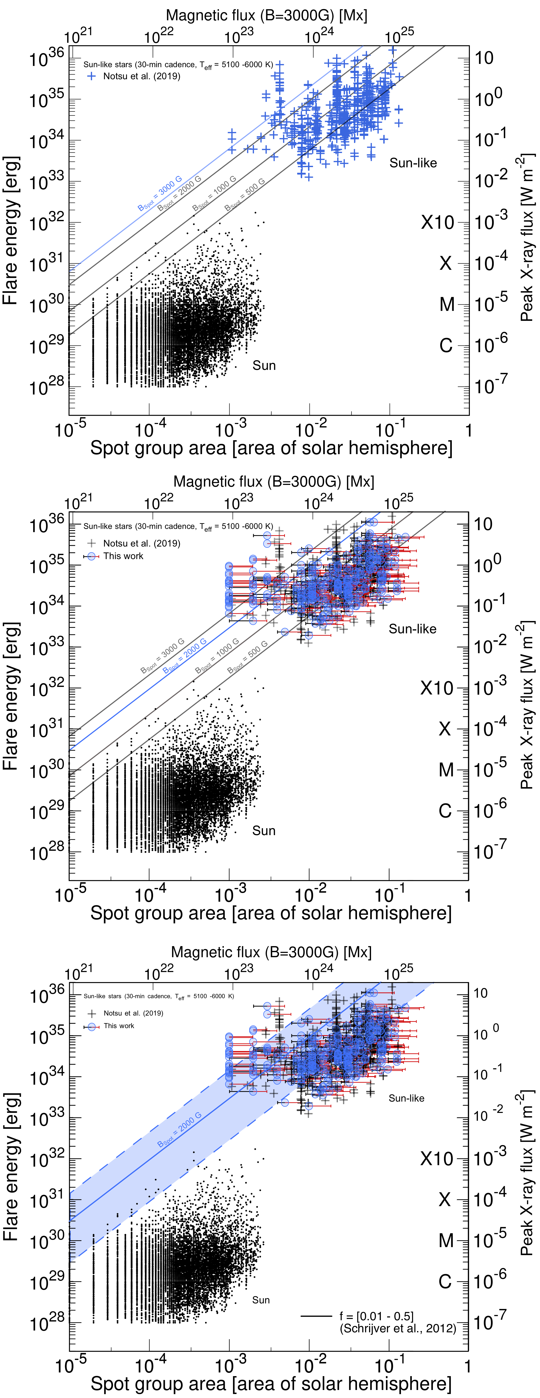
Figure 3: Upper panel: Scatter plot of the flare energy as a function of spot area for solar flares (black dots) and superflares of G-type stars (Notsu et al., 2019). Middle panel: Updated stellar sample by Notsu et al. (2019) based on the newly-derived $\frac{\Delta F}{F_{\mathrm{Star}}}$. Lower panel: Influence of the utilized $f$-values. Upper and lower limits according to Schrijver et al. (2012) [f = 0.01 - 0.5].

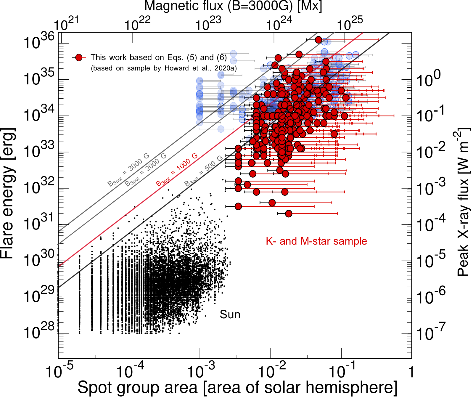
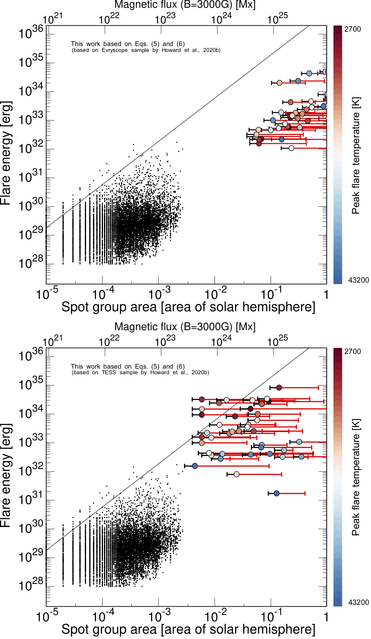
Figure 4: Upper panel: Updated K- and M-star sample of the narrow-band observations of the Evryscope instrument (Howard et al., 2020a). Middle panel: 42 superflares of K5-M5 dwarfs most recently observed with the Evryscope instrument (Howard et al., 2020b). Color-coding corresponds to the measured peak flare intensities. Lower panel: Same superflares observed by TESS.

Additionally, the upper panel of Fig. 3 shows the stellar Sun-like sample by Notsu et al. (2019) (blue crosses). As discussed by Notsu et al. (2019), most of the stellar superflares are located below the 3000 G line. According to Notsu et al. (2019), stars located above this line are considered to have either a low inclination angle or starspots around the poles. However, by taking into account our updated stellar spot-sizes and the limiting errors, as shown in the middle panel, this picture slightly changes. In particular, by taking into account the upper spot group area limits (red error bars) almost all stars of the G-type star sample are found to be well below the 3000 G line, with the majority of stars even located below the 2000 G line, which strongly suggests that the upper limit of the energy released by the observed flares does not exceed the threshold of the magnetic energy stored around the starspots. However, since the utilized $f$-values have a strong impact on the estimated upper flare energy limits, with values discussed in literature ranging from 0.01 to 0.5 and higher, Eqs. (9) and (10) represent only very rough upper estimates (see the lower panel of Fig. 3).

In the case of the K- and M-star regime observed with the narrow-band Evryscope instrument (Howard et al., 2020a), however, the differences between the previously published and the newly-derived upper limits of the flare energy release are more severe (see upper panel of Fig. 4). According to Howard et al. (2020a) the entire sample lies to the right of the 2000 G line, while the majority can be found to the right of the 500 G contour. Based on Eq. (6), however, this picture changes. As can be seen cool stars with $B$-values above the 3000 G line can be found, while the majority of stars is located to the right of the 1000 G line, which is in good agreement with both the measured magnetic field strengths of cool stars (above 4000 G, e.g. Shulyak et al., 2017, 2019) as well as the updated G-type sample by Notsu et al. (2019).

For the Sun-like stellar sample discussed previously, Notsu et al. (2019) follow Shibayama et al. (2013) to estimate the total energy of each flare from the stellar luminosity, amplitude, and duration of flares by assuming that the spectrum of white-light flares can be described by a blackbody radiation with an effective flare temperature of $T_{\rm{flare}}$ = 10,000 K (Mochnacki & Zirin, 1980; Hawley & Fisher, 1992). However, Howard et al. (2020b) most recently published multi-band observations of 42 superflares from 27 K5 - M5 stars. For the first time, a systematic exploration of the superflare temperature evolution is provided, showing constrained blackbody temperatures of flares ranging above 14,000 K up to 42,000 K. While the middle panel of Fig. 4 displays the observations of the narrow-band Evryscope instrument and the corresponding estimations based on Eq. (5) and (6), the lower panel shows the results for the simultaneously observed superflares by TESS (broad-band observations, data taken from Howard et al., 2020b). However, these values should be treated with caution since Howard et al. (2020b) did not consider that the optical emission from K- and M-star flares usually deviate from blackbody spectra (e.g., Fig. 16 of Kowalski et al., 2019) because of the significant contribution from chromospheric emission lines in the visible band (e.g., hydrogen Balmer lines and He I).

Comparing both samples shows that the energies released in the superflares are comparable between the bandpasses. However, because Evryscope uses a narrow bandpass in ”blue” wavelength (4000-5500Å), where the contrast between spot and photosphere is larger than in broad-band observations, the observed amplitudes are in the order of one magnitude higher, and so are the observed $\Delta T/T$-values and the estimated spot group areas.

5 From Stellar Flares to Coronal Mass Ejections

The total flare energy can further be scaled with the energy released in an associated CME. It is known, that fast and energetic CMEs induce shocks in the corona that serve as sites of gradual SEP events with the flux of accelerated protons to energies of a few GeV (Gopalswamy et al., 2005; Fu et al., 2019).

According to Takahashi et al. (2016) the CME mass ($M_{\rm{CME}}$), the CME speed ($v_{\rm{CME}}$), and the corresponding released energetic peak proton flux ($F_{p}$) are related to $E_{\rm{flare}}$ based on simple power-law relations. However, three assumptions have to be made: (1) $M_{\rm{CME}}$ is defined as the sum of all mass within the gravitationally stratified coronal active region, (2) the kinetic energy of the CME is proportional to $E_{\mathrm{flare}}$, and thus

$$E_{\mathrm{CME}}=\frac{1}{2}M_{\mathrm{CME}}V_{\mathrm{CME}}^{2}\propto E_{\mathrm{flare}}=f\frac{B^{2}}{8\pi}A_{\text{spot }}^{3/2},$$ (11)

Therefore, the following dependencies can be derived: $v_{\mathrm{CME}}\propto E_{\rm{flare}}^{1/6}\propto F_{\rm{SXR}}^{1/6}\propto F_{p}^{1/5}$, where $F_{\rm{SXR}}$ is the soft X-ray flux and $F_{\rm{p}}$ the stellar proton flux released in a flare. Thus, $F_{p}$ can be assumed to be proportional to $E_{\rm{flare}}^{5/6}$, and therefore

$$F_{p}\propto\left(4.427\times 10^{34}\cdot f\cdot B\cdot\left(\frac{A_{\rm{Spot}}}{2\pi R_{\odot}^{2}}\right)^{3/2}\right)^{5/6}.$$ (12)

Consequently, based on the latter, the proton flux of particularly M-stars utilizing the previously reported upper magnetic field strength values would be underestimated by about 40%.

6 Summary and Conclusions

The motivation of this study was to investigate the emperical relation between stellar effective temperatures and the temperatures of starspots and the relations for eruptive events based on it.

To this end we utilized the stellar sample by Berdyugina (2005), and proposed a new empirical relation (Eqs. (3) and (4)), for the first time providing a corresponding error-band.

Further, the original stellar sample has been extended. By utilizing the measurements of K- and G-type star sample by Biazzo et al. (2006) and the modeled values of the K-, F-, and G-type star sample by Valio (2017) a new semi-analytic relation is derived that can be applied for all cool star types (Eqs. (5) and (6)). As a result, the newly-derived $\Delta T(T_{\mathrm{Star}})$-values vary between 500 K in the case of cool M-stars (M4) up to about 1500 K in the case of G-type stars (G0). Consequently, the higher-contrast of spots with respect to the photosphere of hotter stars not necessarily is as pronounced as previously thought.

The difference between stellar effective temperatures and starspot temperatures further is often used to derive the size of starspots on the stellar surface (see, e.g., Notsu et al., 2013; Maehara et al., 2017; Notsu et al., 2019; Howard et al., 2020a). It showed that the average difference of the derived $A_{\rm{Spot}}/A_{\rm{Star}}$-values based on the former relations by Berdyugina (2005) and the newly-derived relation discussed in this study is in the order of 20% in the case of G-type stars while being up to 40% in the case of M-type stars, which implies that previous studies most likely underestimated the starspot sizes of cool stars.

In addition, the magnetic energy stored around starspots is often released in the form of stellar flares. According to Sturrock et al. (1984), Shibata et al. (2013) and Notsu et al. (2019), the upper limit of the total energy released in a flare $E_{\text{flare}}$ can be described as constant fraction of the magnetic field energy of the active region (see Emslie et al., 2012), and thus as a rather simple scaling-law. For the G-type star sample reported by Notsu et al. (2019), we found that the stellar magnetic fields of at least 2000 G are most consistent with the measurements. The latter reduces the previously published upper limit by about 1000 G. In addition, Howard et al. (2020a) found that stellar magnetic fields of at least 500 G are most consistent with the narrow-band observations of the Everyscope instrument. Applying the newly-derived correlations, in this study we found that the upper limit of the M-star flare sample most likely is around 1000 G.

We further note, that flares with much lower energy releases are to be expected, however, are not present in the observations due to detection limitations. Solar observations by the Sphinx instrument (about 100 times more sensitive than the GOES instrument), for example, lead to the detection of flares much smaller than the previously known flare classes (S and Q-class flares, see Gryciuk et al., 2017). In addition, recent TESS observations of the M-star GJ 887 showed multiple M- to X-class flares (Loyd et al., 2020) often observed at the Sun.

Nevertheless, the relationships we proposed in this study require further observations (e.g., using instruments like the XMM-Newton and NICER) and numerical modeling of starspot temperatures for G-M dwarfs, which allow an extended empirical characterization of the stellar relationships using all available observational data at hand. The latter will be subject of future investigations.

References

- Airapetian et al. (2016) Airapetian, V. S., Glocer, A., Gronoff, G., Hébrard, E., & Danchi, W. 2016, Nature Geoscience, 9, 452. https://doi.org/10.1038/ngeo2719
- Airapetian et al. (2020) Airapetian, V. S., Barnes, R., Cohen, O., et al. 2020, International Journal of Astrobiology, 19, 136–194. https://doi.org/10.1017/S1473550419000132
- Aschwanden et al. (2014) Aschwanden, M. J., Xu, Y., & Jing, J. 2014, ApJ, 797, 50. https://doi.org/10.1088/0004-637X/797/1/50
- Atri (2019) Atri, D. 2019, Monthly Notices of the Royal Astronomical Society: Letters, 492, L28. https://doi.org/10.1093/mnrasl/slz166
- Aulanier et al. (2013) Aulanier, G., Démoulin, P., Schrijver, C. J., et al. 2013, A&A, 549, A66. https://doi.org/10.1051/0004-6361/201220406
- Basri & Nguyen (2018) Basri, G., & Nguyen, H. T. 2018, The Astrophysical Journal, 863, 190. https://doi.org/10.3847%2F1538-4357%2Faad3b6
- Berdyugina (2002) Berdyugina, S. 2002, Astronomische Nachrichten, 323, 192. https://onlinelibrary.wiley.com/doi/abs/10.1002/1521-3994%28200208%29323%3A3/4%3C192%3A%3AAID-ASNA192%3E3.0.CO%3B2-U
- Berdyugina (2005) Berdyugina, S. V. 2005, Living Reviews in Solar Physics, 2. https://doi.org/https://doi.org/10.12942/lrsp-2005-8
- Berger et al. (2018) Berger, T. A., Huber, D., Gaidos, E., & van Saders, J. L. 2018, The Astrophysical Journal, 866, 99. https://doi.org/10.3847%2F1538-4357%2Faada83
- Biazzo et al. (2006) Biazzo, K., Frasca, A., Catalano, S., et al. 2006, Memorie della Societa Astronomica Italiana Supplementi, 9, 220. https://ui.adsabs.harvard.edu/abs/2006MSAIS...9..220B
- Emslie et al. (2012) Emslie, A. G., Dennis, B. R., Shih, A. Y., et al. 2012, ApJ, 759, 71. https://doi.org/10.1088/0004-637X/759/1/71
- Frasca et al. (2005) Frasca, A., Biazzo, K., Catalano, S., et al. 2005, A&A, 432, 647
- Fu et al. (2019) Fu, S., Jiang, Y., Airapetian, V., et al. 2019, ApJ, 878, L36. https://doi.org/10.3847/2041-8213/ab271d
- Gopalswamy et al. (2005) Gopalswamy, N., Aguilar-Rodriguez, E., Yashiro, S., et al. 2005, Journal of Geophysical Research (Space Physics), 110, A12S07. https://doi.org/10.1029/2005JA011158
- Gryciuk et al. (2017) Gryciuk, M., Siarkowski, M., Sylwester, J., et al. 2017, Sol. Phys., 292, 77. https://doi.org/10.1007/s11207-017-1101-8
- Hawley & Fisher (1992) Hawley, S. L., & Fisher, G. H. 1992, ApJS, 78, 565
- Herbst et al. (2019) Herbst, K., Grenfell, J. L., Sinnhuber, M., et al. 2019, A&A, 631, A101. https://doi.org/10.1051/0004-6361/201935888
- Howard et al. (2019) Howard, W. S., Corbett, H., Law, N. M., et al. 2019, ApJ, 881, 9. https://doi.org/10.3847/1538-4357/ab2767
- Howard et al. (2020a) —. 2020a, ApJ, 895, 140. https://doi.org/10.3847/1538-4357/ab9081
- Howard et al. (2020b) —. 2020b, arXiv e-prints, arXiv:2010.00604
- Kővári et al. (2016) Kővári, Z., Künstler, A., Strassmeier, K. G., et al. 2016, A&A, 596, A53. https://doi.org/10.1051/0004-6361/201628425
- Koch et al. (2010) Koch, D. G., Borucki, W. J., Basri, G., et al. 2010, The Astrophysical Journal, 713, L79. https://doi.org/10.1088%2F2041-8205%2F713%2F2%2Fl79
- Kowalski et al. (2019) Kowalski, A. F., Wisniewski, J. P., Hawley, S. L., et al. 2019, ApJ, 871, 167
- Kriskovics et al. (2019) Kriskovics, L., Kővári, Z., Vida, K., et al. 2019, A&A, 627, A52. https://doi.org/10.1051/0004-6361/201834927
- Kurucz (1991) Kurucz, R. L. 1991, in Precision Photometry: Astrophysics of the Galaxy, ed. A. G. D. Philip, A. R. Upgren, & K. A. Janes, 27. https://ui.adsabs.harvard.edu/abs/1991ppag.conf...27K
- Livingston & Watson (2015) Livingston, W., & Watson, F. 2015, Geophys. Res. Lett., 42, 9185. https://doi.org/10.1002/2015GL065413
- Loyd et al. (2020) Loyd, R. O. P., Shkolnik, E. L., France, K., Wood, B. E., & Youngblood, A. 2020, Research Notes of the AAS, 4, 119. https://doi.org/10.3847%2F2515-5172%2Faba94a
- Maehara et al. (2017) Maehara, H., Notsu, Y., Notsu, S., et al. 2017, Publications of the Astronomical Society of Japan, 69, doi:10.1093/pasj/psx013, 41. https://doi.org/10.1093/pasj/psx013
- Maehara et al. (2012) Maehara, H., Shibayama, T., Notsu, S., et al. 2012, Nature, 485, 478. https://doi.org/10.1038/nature11063
- McQuillan et al. (2014) McQuillan, A., Mazeh, T., & Aigrain, S. 2014, The Astrophysical Journal Supplement Series, 211, 24. https://doi.org/10.1088/0067-0049/211/2/24
- Mekhaldi et al. (2015) Mekhaldi, F., Muscheler, R., Adolphi, F., et al. 2015, Nature Communications, 6, 8611. https://doi.org/10.1038/ncomms9611
- Miyake et al. (2012) Miyake, F., Nagaya, K., Masuda, K., & Nakamura, T. 2012, Nature, 486, 240. https://doi.org/10.1038/nature11123
- Mochnacki & Zirin (1980) Mochnacki, S. W., & Zirin, H. 1980, ApJ, 239, L27
- Morris et al. (2018) Morris, B. M., Agol, E., Davenport, J. R. A., & Hawley, S. L. 2018, MNRAS, 476, 5408. https://doi.org/10.1093/mnras/sty568
- Namekata et al. (2019) Namekata, K., Maehara, H., Notsu, Y., et al. 2019, The Astrophysical Journal, 871, 187. https://doi.org/10.3847%2F1538-4357%2Faaf471
- Namekata et al. (2020) Namekata, K., Davenport, J. R. A., Morris, B. M., et al. 2020, ApJ, 891, 103
- Notsu et al. (2013) Notsu, Y., Shibayama, T., Maehara, H., et al. 2013, ApJ, 771, 127. https://doi.org/10.1088/0004-637x/771/2/127
- Notsu et al. (2019) Notsu, Y., Maehara, H., Honda, S., et al. 2019, The Astrophysical Journal, 876, 58. https://doi.org/10.3847/1538-4357/ab14e6
- O’Hare et al. (2019) O’Hare, P., Mekhaldi, F., Adolphi, F., et al. 2019, Proceedings of the National Academy of Science, 116, 5961. https://doi.org/10.1073/pnas.1815725116
- O’Neal et al. (2004) O’Neal, D., Neff, J. E., Saar, S. H., & Cuntz, M. 2004, AJ, 128, 1802. https://doi.org/10.1086/423438
- Özdarcan et al. (2016) Özdarcan, O., Carroll, T. A., Künstler, A., et al. 2016, A&A, 593, A123. https://doi.org/10.1051/0004-6361/201628545
- Panja et al. (2020) Panja, M., Cameron, R., & Solanki, S. K. 2020, The Astrophysical Journal, 893, 113. https://doi.org/10.3847%2F1538-4357%2Fab8230
- Prusti et al. (2016) Prusti, T., de Bruijne, J. H. J., Brown, A. G. A., et al. 2016, A&A, 595, A1. https://doi.org/10.1051/0004-6361/201629272
- Ricker et al. (2015) Ricker, G. R., Winn, J. N., Vanderspek, R., et al. 2015, Journal of Astronomical Telescopes, Instruments, and Systems, 1, 014003. https://doi.org/10.1117/1.JATIS.1.1.014003
- Sammis et al. (2000) Sammis, I., Tang, F., & Zirin, H. 2000, The Astrophysical Journal, 540, 583. https://doi.org/10.1086%2F309303
- Scheucher et al. (2020) Scheucher, M., Herbst, K., Schmidt, V., et al. 2020, The Astrophysical Journal, 893, 12. https://doi.org/10.3847%2F1538-4357%2Fab7b74
- Schrijver et al. (2012) Schrijver, C. J., Beer, J., Baltensperger, U., et al. 2012, Journal of Geophysical Research (Space Physics), 117, A08103. https://doi.org/10.1029/2012JA017706
- Shibata et al. (2013) Shibata, K., Isobe, H., Hillier, A., et al. 2013, PASJ, 65, 49. https://doi.org/10.1093/pasj/65.3.49
- Shibayama et al. (2013) Shibayama, T., Maehara, H., Notsu, S., et al. 2013, The Astrophysical Journal Supplement Series, 209, 5. https://doi.org/10.1088/0067-0049/209/1/5
- Shulyak et al. (2017) Shulyak, D., Reiners, A., Engeln, A., et al. 2017, Nature Astronomy, 1, 0184. https://doi.org/10.1038/s41550-017-0184
- Shulyak et al. (2019) Shulyak, D., Reiners, A., Nagel, E., et al. 2019, A&A, 626, A86. https://doi.org/10.1051/0004-6361/201935315
- Stassun et al. (2019) Stassun, K. G., Oelkers, R. J., Paegert, M., et al. 2019, The Astronomical Journal, 158, 138. https://doi.org/10.3847/1538-3881/ab3467
- Strassmeier et al. (2019) Strassmeier, K. G., Carroll, T. A., & Ilyin, I. V. 2019, A&A, 625, A27. https://doi.org/10.1051/0004-6361/201834906
- Sturrock et al. (1984) Sturrock, P. A., Kaufman, P., Moore, R. L., & Smith, D. F. 1984, Sol. Phys., 94, 341. https://doi.org/10.1007/BF00151322
- Takahashi et al. (2016) Takahashi, T., Mizuno, Y., & Shibata, K. 2016, The Astrophysical Journal, 833, L8. https://doi.org/10.3847/2041-8205/833/1/l8
- Toriumi et al. (2020) Toriumi, S., Airapetian, V. S., Hudson, H. S., et al. 2020, The Astrophysical Journal, 902, 36. https://doi.org/10.3847%2F1538-4357%2Fabadf9
- Toriumi & Wang (2019) Toriumi, S., & Wang, H. 2019, Living Reviews in Solar Physics, 16, 3
- Valio (2017) Valio, A. 2017, in IAU Symposium, Vol. 328, Living Around Active Stars, ed. D. Nandy, A. Valio, & P. Petit, 69–76. https://doi.org/10.1017/S1743921317004094
- Yamashiki et al. (2019) Yamashiki, Y. A., Maehara, H., Airapetian, V., et al. 2019, ApJ, 881, 114. https://doi.org/10.3847/1538-4357/ab2a71