SMSupplemental Material

Ab initio modeling and experimental investigation of Fe₂P by DFT and spin spectroscopies

Abstract

Fe₂P alloys have been identified as promising candidates for magnetic refrigeration at room-temperature and for custom magnetostatic applications. The intent of this study is to accurately characterize the magnetic ground state of the parent compound, Fe₂P, with two spectroscopic techniques, $\mu$SR and NMR, in order to provide solid bases for further experimental analysis of Fe₂P-type transition metal based alloys. We perform zero applied field measurements using both techniques below the ferromagnetic transition $T_{C}=220$ K. The experimental results are reproduced and interpreted using first principles simulations validating this approach for quantitative estimates in alloys of interest for technological applications.

Introduction.

Fe₂P-based alloys have attracted significant research interest in recent years owing to their first-order magnetic transition (FOMT) coupled to a magnetoelastic transition, giving rise to a giant magnetocaloric effect in the vicinity of their Curie temperature [1], which is tunable across room temperature by suitable Fe-Mn and P-Si, P-B substitution [2, 3]. The latter, along with their composition by cheap and abundant elements, makes them eligible for energy transduction applications including solid-state harvesting of thermal energy [4, 5] and real-case magnetocaloric refrigerators, that provide increased energy efficiency and substantial environmental benefits compared to gas compression thermodynamic cycles [6, 7, 8, 9].

A FOMT is also shown by the parent compound Fe₂P [10], which however exhibits a much larger magneto-crystalline anisotropy (MCA) than Fe₂P-based FeMnPSi compounds [11], making it rather a candidate material for permanent magnets. Indeed, its Curie temperature ($T_{C}\approx 220~{}\mathrm{K}$) is too low for most applications. However, $T_{C}$ can be raised well above room temperature by suitable Si, Ni, Co alloying while preserving a MCA nearly as large as in the parent compound [12]. It is therefore apparent that pure Fe₂P, though not directly applicable in magnetic or magnetocaloric technology, shares most of its physics with the derived alloys, while it is possibly a simpler system to model theoretically.

Fe₂P crystallizes in the hexagonal C₂₂ structure with a space group $P\bar{6}2m~{}(189)$ and the primitive unit cell contains three formula units and four inequivalent sites, with iron occupying the $3f$ (Fe1) and the $3g$ sites (Fe2) in equal number, and phosphorus occupying sites $2c$ (P1) and $1b$ (P2) in a 2:1 ratio [13, 14]. The compound orders ferromagnetically (FM) with magnetic moments directed along the c-axis. The magnetic structure of Fe₂P has been widely investigated by neutron scattering and Mössbauer spectroscopy [10, 14, 15, 16, 17, 18, 19]. All reports qualitatively agreed on a larger Fe2 moment with a localized character, and a reduced Fe1 moment typical of itinerant magnetism (a feature shared by FeMnPSi alloys [20]). However, poor quantitative agreement on the size of the Fe1 magnetic moment characterized early literature and, in addition, the presence of helical states below $T_{c}$ was discussed [18]. Recently, elastic neutron scattering experiments [21] seem to have finally established the value of the Fe1 and Fe2 moments as 0.8 $\mu_{\mathrm{B}}$ and 2.11 $\mu_{\mathrm{B}}$, respectively. The same experiments also showed absence of canting below $T_{c}$ and the presence of sizable local moments on Fe up to 30 K above the FM transition temperature.

In this work we present an investigation of the magnetically ordered phase and of the magnetic transition of this compound by two local probes of magnetism, namely NMR and $\mu$SR. Both techniques have been used to probe Fe₂P only in their infancy and published results are very limited to the best of our knowledge [22, 23].

In zero applied field (ZF), ³¹P and ⁵⁷Fe nuclei resonate in their hyperfine fields, giving rise to distinct resonance lines for each crystallographic site. We detected the ⁵⁷Fe resonance of Fe2 and the ³¹P resonances of P1 and P2 and unambiguously assigned them to their respective nuclei, thus correcting the peak attribution by an early NMR work [23], which is proven here to be erroneous. The so-determined ³¹P hyperfine fields effectively complement the determination of the ⁵⁷Fe hyperfine fields by Mössbauer spectroscopy [10]. ZF $\mu$SR showed a single sharp precession peak below $T_{C}$, whose low-temperature frequency poses stringent constraints to the stopping site of the implanted muons, while its temperature dependence confirms a FOMT in the system. Experimental results are compared to a simulation of the system by ab initio methods, yielding theoretical predictions for the local fields at the ³¹P, ⁵⁷Fe nuclei and at the muon in its stable interstitial site.

The motivation of this work is threefold. First, the inconsistencies that can be found in the sparse and often very old literature on parent Fe₂P, as pointed out above, demand clarification by newer experiments. Second, this study will guide the interpretation of NMR and $\mu$SR experiments on Fe₂P-based alloys of interest for applications. Third, our results benchmark and validate ab initio investigations that are shown to be extremely useful for experimental data analysis.

Material and methods.

Fe₂P is prepared by firing a mixture of BASF carbonyl iron powder with red phosphorus under protective atmosphere. This mixture reacts exothermally and is very low in transition metal impurities, less than 0.01 %. It was checked by X-ray diffraction to be single phase Fe₂P type.

The NMR experiments were carried out by a home-built phase-coherent spectrometer [24] and a resonant LC probehead, using a field-sweeping cold-bore cryomagnet (Oxford Instruments Maglab EXA) equipped with a helium-flow variable temperature insert and a nitrogen-flow cryostat in zero field as sample environments at $T=5~{}\mathrm{K}$ and $T\geq 80~{}\mathrm{K}$, respectively. ZF measurement at 77.3 K were performed by directly immersing the probehead in a liquid nitrogen dewar. Additional details about the experimental data acquisition are reported in the Supplemental Material (SM) .

$\mu$SR experiments were performed on the LAMPF (Los Alamos Meson Physics Facility) spectrometer at TRIUMF in Vancouver, Canada and the General Purpose Surface-Muon Instrument at the Paul Scherrer Institut (PSI) in Villigen, Switzerland. The loose powder sample of Fe₂P used for the experiment at TRIUMF was loaded into a mylar pouch and placed in a low-background sample holder. $\mu$SR spectra were collected in zero field (ZF) at temperatures between 100 K and 300 K using a helium flow cryostat to control the temperature. A calibration measurement was conducted in a weak transverse field at 275 K. The powder sample used at PSI was mixed with a small amount of wax. ZF spectra were collected at 5 K and 200 K using a helium flow cryostat. At both experimental facilities, data were collected in a warming sequence. Fits to the $\mu$SR spectra were conducted via least-squares optimization using MUSRFIT [25], and a home-built python package called BEAMS, both of which yielded statistically indistinguishable results for the oscillating frequencies.

The magnetic and structural stability of Fe₂P  and of various alloys have been already studied with different computational approaches [26, 27, 28, 12]. We reproduced previously reported results on the FM phase [29, 16, 17, 28] with both plane wave and full-potential approaches using the Quantum ESPRESSO suite of codes, the WIEN2k package and the Elk code respectively [30, 31, 32, 33, 34]. The plane wave and pseudopotential method is essential to reduce the computational effort required for muon site assignment and hyperfine field characterization, while full potential approaches provide superior accuracy for the evaluation of the hyperfine fields at P nuclei. All computational details are reported in the SM .

NMR

.

Figure 1: a) ³¹P(1) NMR spectra at $T=5~{}\mathrm{K}$ in ZF (domain wall signal) and in applied fields approaching saturation of the magnetization (domain signal). The inset shows the resonant frequency vs applied field, the black line is a fit described in main text. b) ZF NMR spectrum at $T=77.3~{}\mathrm{K}$: ³¹P2 (left panel, filled squares), ⁵⁷Fe2 (left panel, empty diamonds) resonance lines and ³¹P1 resonance (right panel, filled circles). In (a-b) the lines are guides to the eye. c) Zero-field $\mu$SR spectrum collected at 5 K. The blue dots represent the experimental data and the solid black curve is a fit obtained through least-squares optimization. The coherent oscillations indicate the presence of a well-defined, static magnetic field at the muon stopping site due to the long-range FM order. d) The static field at the muon stopping site as a function of temperature, obtained from fits to the ZF-$\mu$SR spectra. The vertical dashed line represents the Curie temperature ($\sim$220 K).

Spontaneous ZF NMR signals were detected at low temperature in the 70-90 MHz and the 13-24 MHz frequency intervals, in loose agreement with the frequency bands where similar resonances were reported by Koster and Turrell and assigned therein to ³¹P in P1, P2 and ⁵⁷Fe in Fe1 and Fe2, respectively [23].

The higher-frequency portion of the ZF spectrum at 5 K is plotted in Fig. 1a. The relative high frequency indicates that these resonances stem from ³¹P nuclei (gyromagnetic ratio ${}^{31}\gamma/2\pi=17.2357~{}\mathrm{MH/T}$), since a ⁵⁷Fe resonance at the same frequency (${}^{57}\gamma/2\pi=1.3786~{}\mathrm{MH/T}$) would correspond to hyperfine fields of $\approx 60~{}\mathrm{T}$, whence an unphysical local moment $>5\mu_{B}$ according to the known iron hyperfine coupling [35]. Nuclear spin echoes were excited with shorter and strongly attenuated rf pulses compared to standard NMR in non magnetic compounds, indicative of a large rf enhancement of the resonance [36]. The mean enhancement factor $\eta$ was estimated in the order of 1000 by comparison with the optimum excitation conditions in an intense applied field saturating the magnetization (see below), where $1<\eta<2$ can be assessed [37]. Such a large $\eta$ value prove that these signals originate from nuclei in domain walls .

The ³¹P ZF spectrum of Fig. 1a) exhibits a structure with two cusps at approx. 78 and 88 MHz. Such features were identified with independent resonance peaks and assigned to P2 and P1 by Ref. [23]. However, such an attribution is inconsistent with experiments. First, the enhancement factors for the two spectral features differ by a factor of $\approx 3$ ($\eta$ is larger on the higher frequency side), a difference that cannot be reconciled with two close-frequency peaks in a homogeneous magnetic structure, and rather points to nuclei at different positions inside a domain wall [36, 37]. Moreover, the two-cusp structure progressively disappears in an applied field large enough to saturate the magnetization. The same figure also shows the 5 K spectra from ³¹P nuclei in the bulk of domains, in applied field values $\mu_{0}H^{\prime}=1.8~{}\mathrm{T}$ and $\mu_{0}H^{\prime\prime}=3.5~{}\mathrm{T}$ corresponding to a nearly saturated state and a practically full saturation of the magnetic moment of polycrystalline Fe₂P, respectively [11]. From $H^{\prime}$ to $H^{\prime\prime}$, vector composition of the internal with the external field shifts the resonance frequency as $\delta\nu=\nu^{\prime\prime}-\nu^{\prime}=\mu_{0}(H^{\prime\prime}-H^{\prime})^{31}\gamma/2\pi$, in agreement with ³¹P nuclei with a positive hyperfine coupling, while the lineshape tends to a single Gaussian curve at increasing field. It is therefore apparent that these NMR signals constitute a single resonance line, which is assigned to P1 by the DFT calculations detailed below.

The complex lineshape of the ZF spectrum at 5 K seemingly stems from the anisotropic component of the hyperfine coupling and the particular (though unknown) micromagnetic structure of domain walls, whereby spins inside a wall do not sample the solid angle with equal probability. A uniform angle sampling relative to crystal axes, on the contrary, is approached by saturating the magnetization of the polycrystalline specimen. The linewidth of the spectrum in the larger applied field is estimated as $\Delta\nu=4.6~{}\mathrm{MHz}$, whence a rms anisotropic hyperfine field $B_{hf}^{(anis)}=\sqrt{3}\Delta\nu\,2\pi/{{}^{31}\gamma}=0.46(1)~{}\mathrm{T}$. The isotropic hyperfine field at this site can be estimated from the first moment of the spectrum $B_{hf}^{(iso)}=2\pi\bar{\nu}/{{}^{31}\gamma}=4.7(1)\mathrm{T}$, a result that however suffers from the uncertainty on the details of domain walls. A different estimate is obtained from the dependency of the resonant frequency on the applied field. The fit shown in the inset of Fig. 1a), where $\nu(0)$ is the only free parameter, provides $B_{hf}^{(iso)}=2\pi\nu(0)/{{}^{31}\gamma}=3.83(4)$ T.

At higher temperature, the ³¹P(1) ZF spectrum evolves to a single narrower peak. The two-cusp structure has already disappeared at 77.3 K (Fig. 1b), where only a weaker Gaussian shoulder can be detected besides the main peak at 72.6 MHz, and the overall spectral width is estimated as $\Delta\nu=1.1(1)~{}\mathrm{MHz}$. The narrowing of the ZF spectrum witnesses a decrease of the anisotropic hyperfine coupling of P1 from 5 to 77.3 K. On further warming, the mean resonance frequency vs temperature follows a smooth order parameter curve, with $\bar{\nu}(T)$ values in good agreement with the literature, up to 160 K [23]. Above that temperature, the signal is lost due to exceedingly fast relaxations, and the magnetic transition cannot be probed by NMR.

Lower-frequency resonances, shown in Fig. 1b), were investigated at 77.3 K. The ZF NMR spectrum features a broad, more intense composite line at 14-18 MHz, and a weaker asymmetric peak at 23.7 MHz. The latter value is in excellent agreement with a ⁵⁷Fe resonance in the hyperfine field of 17.2 T reported by ⁵⁷Fe Mössbauer spectroscopy for Fe2 at this temperature [10], which warrants the same assignment for this NMR line. The other broader resonance is however incompatible with the ⁵⁷Fe NMR of Fe1, although such a resonance line is predicted at 15.0 MHz ($B_{hf}=10.9~{}\mathrm{T}$) by the same Mössbauer data. In fact, the same integrated amplitude (after normalization by $\nu^{2}$) would be expected in that case for the two signals, given the 1:1 Fe occupancy ratio at the two sites. The 14-18 MHz signal must therefore originate from the resonance of the much more sensitive ³¹P nuclei in a mean spontaneous field of 0.94(4) T at the complementary P2 site, while the weaker and overlapped ⁵⁷Fe(1) line is hidden by it. Our assignment, which contrasts with early literature [23], is also further confirmed by the relative receptivity of the two nuclear species as detailed in the SM .

The ³¹P(2) spectrum at 77.3 K exhibits a similar structure as the one observed at 5 K in the ³¹P(1) one, which can be explained based on similar arguments. Its linewidth and the P2 rms anisotropic hyperfine field are estimated as $\Delta\nu=1.8(1)~{}\mathrm{MHz}$ and $B_{hf}^{(anis)}=\sqrt{3}\Delta\nu\,2\pi/{{}^{31}\gamma}=0.18(1)~{}\mathrm{T}$, hence they are significantly larger, both in absolute and relative terms, than the corresponding P1 values at the same temperature.

$\mu$SR

. In Fig. 1c), we display the ZF-$\mu$SR spectrum collected at 5 K. The blue dots represent the experimental asymmetry as a function of time. Well-defined oscillations with a single dominant frequency are clearly visible, confirming the presence of a static and fairly uniform magnetic field at the muon stopping site. An excellent fit to the spectrum is obtained using the standard two-component model expected for static internal fields, consisting of an exponentially damped sinusoidal function and a slowly relaxing exponential function, as shown by the black curve in Fig. 1c). At 5 K, the best-fit frequency is $\nu=53.72(1)$ MHz, corresponding to a magnetic field magnitude of $B_{\mu}=\nu/\gamma_{\mu}=0.3963(1)$ T, where $\gamma_{\mu}=135.5~{}\mathrm{MHz~{}T^{-1}}$ is the gyromagnetic ratio of the muon. Equivalent fits were performed for the ZF spectra collected at temperatures up to $T_{c}\sim 220$ K, while above $T_{c}$ a pure exponential decay is observed.

The local static field at the muon site extracted from these fits is displayed as a function of temperature in Fig. 1c), with blue circles and orange triangles representing the results from data collected at TRIUMF and PSI respectively. Excellent agreement is found between the TRIUMF and PSI results. As the temperature increases toward $T_{c}$, the static field steadily decreases, as expected for a magnetic order parameter curve. At approximately 220 K (indicated by the vertical dashed line in Fig. 1d), however, the static field drops discontinuously to zero, indicating the occurrence of a first-order magnetic transition at this temperature. A fast depolarization (not shown) is observed well above $T_{c}$, indicating the presence of short range correlations in agreement with previous neutron scattering results.

Computational results.

In order to further characterize the microscopic origin of the experimental results and to validate ab initio estimates of hyperfine couplings, we evaluated the internal field at P and the muon sites, after having identified the interstitial position occupied by the latter following a methodology already extensively discussed [39, 40, 41, 42, 43, 44, 45, 46, 47, 48].

Label	Wyckoff	$(x,y,z)$	$\Delta E(meV)$	$B_{C}$ (T)
A	$3g$	(0.000, 0.328, 0.500)	0	-0.4274
A*	$6k$	(0.052, 0.358, 0.500)	0	-0.5022
B	$3f$	(0.296, 0.296, 0.000)	280	-0.4573
C	$2d$	(0.333, 0.666, 0.500)	690	-1.7049
D	$3f$	(0.000, 0.545, 0.009)	760	-
E	$1a$	(0.000, 0.000, 0.000 )	1120	-

Table 1: Muon sites and contact hyperfine fields obtained ab initio. The second and third columns report the position of the candidate muon sites in fractional coordinates with respect to a unit cell where Fe1 occupies the $3f$ position in (0.0,0.257,0.0) and Fe2 the $3g$ position in (0.0, 0.591, 0.5). The total energy differences $\Delta E=E_{i}-E_{A}$ and the contact hyperfine field at each site are in fourth and fifth columns.

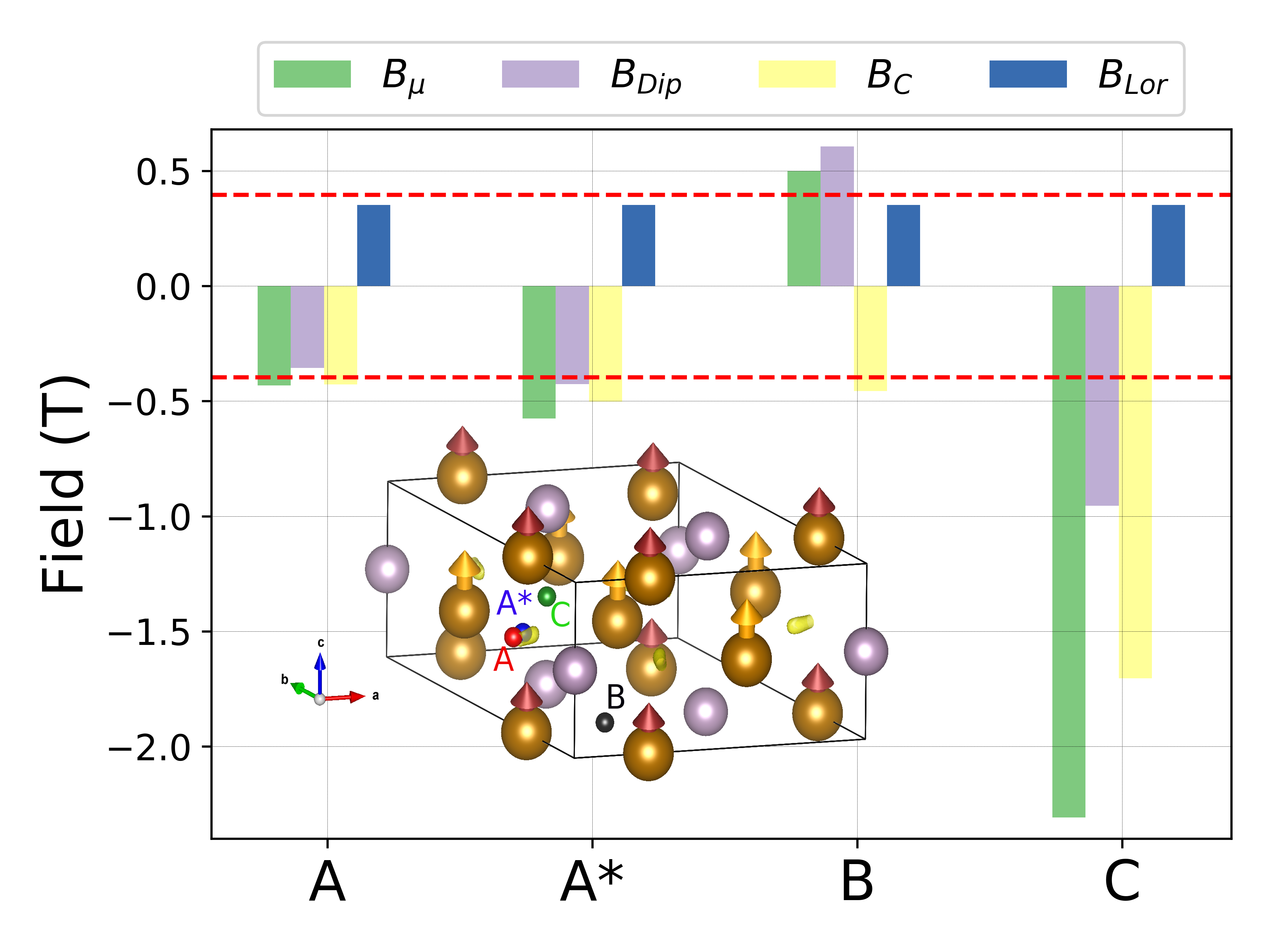
Figure 2: Local field at the muon sites along the $\mathbf{c}$ lattice vector. The green bar is the sum of the LR dipolar (gray and blue), and Fermi contact (yellow) contributions. The red dashed line shows $\pm B_{\mu}$ (see text). The inset shows the Fe₂P unit cell where on Fe atoms (brown) the short(long) red(orange) arrows identify the small(large) Fe1(Fe2) magnetic moments. P atoms are big mauve spheres and muon sites are the small spheres labeled A, A* , B and C. The yellow isosurfaces represent 0.2 eV above the minimum of the unperturbed electrostatic potential.

Five inequivalent candidate muon sites, labeled with letters from A to E in order of increasing total energy, are reported in Tab. 1. The label A* indicates a slightly displaced analogous of site A, with the distance $d_{A-A*}$ being 0.2 Å. The energy difference between the two is within numerical accuracy, but their distance testifies a rather flat potential energy surface that implies some degree of delocalization of the muon wave-function.

Notably, the positions A and B are just $0.5$ Å and 0.3 Å away from the absolute minimum and the second lowest minimum of the electrostatic potential while site C corresponds exactly to the position of the third relative minimum of the electrostatic potential. A similar behavior was found in muon site calculations performed on FeCrAs that shares the same spacegroup with Fe₂P[49]. Finally, the largest displacement induced by the muon on the neighboring magnetic atoms is smaller than $0.15$Å.

In a ZF NMR or $\mu$SR experiment performed below $T_{C}$, the effective field at the nuclei or muon can be separated into multiple contributions:

$$\mathbf{B}_{\mathrm{Tot}} =\mathbf{B}_{\mathrm{LR}}+\mathbf{B}_{\mathrm{Demag}}+\mathbf{B}_{\mathrm{SR}}$$ (1)

$$\mathbf{B}_{\mathrm{LR}} =\mathbf{B}_{\mathrm{Lor}}+\mathbf{B}_{\mathrm{Dip}}$$ (2)

$$\mathbf{B}_{\mathrm{SR}} =\mathbf{B}_{\mathrm{C}}+\mathbf{B}_{\mathrm{DipSR}}+\mathbf{B}_{\mathrm{OrbSR}}$$ (3)

The first term in Eq. 1 is the long range (LR) dipolar field which is obtained here in real space using the Lorentz method, in which the magnetic moment of Fe $3d$ orbitals inside a (large) sphere contribute to $\mathbf{B}_{\mathrm{Dip}}$ while those outside it are treated as a continuum and add into $\mathbf{B}_{\mathrm{Lor}}$ appearing in Eq. 2. $\mathbf{B}_{\mathrm{Demag}}$ is the demagnetization field, that can be neglected in a polycrystalline and multidomain sample, and $\mathbf{B}_{\mathrm{SR}}$ is the short range term arising from orbitals localized at the muon or P site, which is further subdivided, in order of appearance in Eq. 3, in the Fermi contact, dipolar and orbital terms.

For the LR dipolar field we approximate the spin polarization of Fe $d$ orbitals as classical magnetic moments with $m_{\mathrm{Fe1}}=0.84$ $\mu_{\mathrm{B}}$ and $m_{\mathrm{Fe2}}=2.22$ $\mu_{\mathrm{B}}$ both along $c$.

Code	Nuc.	$B_{\mathrm{C}}$	$B_{\mathrm{DipSR}}$	${B}_{\mathrm{Dip}}$	$B^{\mathrm{(iso)}}_{\mathrm{exp}}$	$\sqrt{5/2}B^{\mathrm{(anis)}}_{\mathrm{exp}}$
WIEN2k	P1	3.8	-1.0	+ 0.11	$3.83(4)^{\dagger}$	$0.73(2){\dagger}$
	P2	0.3	0.2	- 0.19	$0.94(4)^{\star}$	$0.28(2)^{\star}$
Elk	P1	4.0/3.2	-0.8	+0.11	$3.83(4)^{\dagger}$	$0.73(2)^{\dagger}$
	P2	0.2/0.7	0.1	-0.19	$0.94(4)^{\star}$	$0.28(2)^{\star}$

• ^† data from applied field NMR; ^⋆ data from ZF NMR.

Table 2: Hyperfine fields at the P nuclei in the low temperature FM phase. A positive contact field indicates that the spin polarization of a given contribution is oriented like Fe-$d$ orbitals, a negative sign means the opposite. The two values reported for $B_{C}$ in the second row are the results of two different algorithms used to compute the contact part (see SM). The fourth and fifth columns report the principal component of the dipolar tensor. All values are in Tesla and the Lorentz contribution to the long range dipolar field is 0.35 T.

The occupied orbitals with non-negligible electronic density at the muon sites consist mainly of s-character and relativistic effects can be safely neglected. In this approximation, the short-range contribution (Eq. 3) is limited to the contact term, that is estimated from the electronic spin polarization at the muon position $\bm{R}_{l}$ as $B_{\mathrm{SR}}=\frac{2}{3}\mu_{0}\mu_{B}\rho_{s}(\bm{R}_{l})$ [50, 42] where $\rho_{s}(\bm{R}_{l})$ is the spin density at the muon site. We can therefore compute $\mathbf{B}_{\mathrm{Tot}}(\bm{R}_{l})$ entirely from first principles and the results are shown in Fig. 2 [51]. The long range dipolar contributions is negligible for both the lowest energy sites A and B, where the local field originates from the Fermi contact term. The comparison with the experimentally measured local field is excellent and equally good for both sites, with the former showing slightly better agreement.

A similar approach is used to estimate the local field at P sites, where however relativistic effects must be considered [52]. The contact term in this case dramatically depends on valence electrons’ spin polarization and an accurate description of the latter is mandatory. The short-range dipolar and orbital contributions are estimated differently by Elk and WIEN2k (see SM), but in both cases $B_{\mathrm{OrbSR}}$ is negligible and therefore not reported.

The calculated hyperfine field at P1 and P2 sites shown in Tab 2 provides the attribution of the NMR peaks already discussed. The contact term accurately reproduces the experimental bulk $B_{hf}^{(iso)}$ for P1 while the comparison for P2 is seemingly less accurate. However, an uncertainty of the order of the Lorentz term has to be considered since the experimental estimate for P1 is from domain wall signal and, notably, the difference between bulk and wall signals for P2 is 0.9 T. The analysis of the anisotropic part requires more care. In Tab 2 the experimental $B_{hf}^{(aniso)}$ is multiplied by $\sqrt{5/2}$ in order to compare it with the largest principal value of the dipolar tensor. In ZF, the uncertainty stemming from the unknown nature of the domain walls impairs a precise theoretical determination. In applied field, at saturation, $B_{\mathrm{Lor}}$ and $B_{\mathrm{Demag}}$ cancel out and, for Fe₂P, only $B_{\mathrm{DipSR}}$ and $B_{\mathrm{Dip}}$ contribute to the anisotropic part. A good quantitative agreement is obtained in this case for P1.

Conclusions.

We investigated the FM phase of Fe₂P using in-field and zero-field ³¹P NMR and $\mu$SR, characterizing in detail both experimental signals in the low temperature magnetic phase. First principles simulations unveiled the interstitial position occupied by the muon and provided hyperfine parameters for P nuclei and the muon, accurately reproducing the experimental results. This information provides a framework for the analysis of future experiments on Fe₂P alloys of technological interest.

Supplementary Material for “Ab initio modeling and experimental investigation of Fe₂P by DFT and spin spectroscopies”

.1 NMR

The NMR spectra were reconstructed point by point by exciting spin echoes at discrete frequencies. The corresponding spectral amplitude were determined as the zero-shift Fourier component of the echo signal, divided by the frequency-dependent sensitivity $\propto\omega^{2}$. At each frequency step, the LC resonator was re-tuned by a servo-assisted automatic system plugged into the spectrometer. A standard $P-\tau-P$ spin echoes pulse sequence was employed, with equal rf pulses $P$ of intensity and duration optimized for maximum signal, and delay $\tau$ as short as possible, compatibly with the dead time of the apparatus.

A further check of the assignment of the 14-18 MHz signal to ³¹P nuclei, which contrasts with early literature SM_10.1063/1.1660234, is obtained from the relative receptivity $R=R^{\prime}B_{hf}=a\gamma^{3}B_{hf}^{3}=a\omega^{3}$ of the two nuclear species. Here $R^{\prime}=a\gamma^{3}B^{2}$ is the usual dependence of the sensitivity of a nucleus on its abundance $a$ (both isotopic and from site multiplicity) and the local field $B$ in a non-magnetic substance, whereas in a ferromagnet a further dependency on $B=B_{hf}$ arises from the enhancement factor Riedi_eta, Panissod. After normalization of the spectra by $\omega^{2}$ (the amplitude correction appropriate for the signals of a single nuclear species), the integrated amplitudes $A$ of the ³¹P and ⁵⁷Fe signals should scale relative to each other as $R_{n}=a\omega$, whence an expected ratio ${}^{31}R_{n}/{}^{57}R_{n}=11$, in fair agreement with the value ${}^{31}A/{}^{57}A\approx 16$ that we estimated experimentally. A direct comparison between the ³¹P NMR amplitudes at P1 and P2 is not possible due to the large difference in frequency whence the employment of different resonant circuits.

The shape of the 77.3 K spectrum, testifying a variation of the anisotropic hyperfine coupling, was checked against different spin-echo excitation conditions (selecting nuclei with different enhancement factors)Panissod_Nato and was found to be independent of rf pulse amplitude over more than two decades.

.2 DFT simulation details

The magnetic ground state of Fe₂P is accurately reproduced by the Perdew-Burke-Ernzerhof (PBE) exchange and correlation functional SM_PERDEWPBE1996. The energy difference between the ferromagnetic and the spin-degenerate case is $1.1$ eV per unit cell and the magnetic moment of Fe1 is found to be 0.84 $\mu_{\mathrm{B}}$ while that of Fe2 is 2.22 $\mu_{\mathrm{B}}$. Both these results are in agreement with previous computational studies and compare extremely well with experimental findings.SM_Tobola1996, SM_KOUMINA1998, SM_Ishida1987, SM_Bhat2018

The lattice structure of Fe₂P  was taken from the crystallographic information file deposited on the COD database SM_Quiros2018 with ID: 9012616.

In the simulations using plane wave and pseudopotential, the basis set was expanded up to a cutoff of 80 Ry while charge density up to 800 Ry. A uniform Monkhorst-Pack (MP) SM_MONKHORST1976 mesh of $6\times\ 6\times 8$ was used for sampling the reciprocal space in the unit cell while we used a $2a\times 2b\times 3c$ supercell to identify muon interstitial sites.

In the optimization of the structure and description of magnetic properties a Marzari-Vanderbilt SM_MARZARI1999 smearing of 5 mRy was used while a Gaussian smearing of 20 mRy is chosen for supercell calculations.

The experimental lattice parameters $a=b=5.877$ and $c=3.437$Å SM_SENATEUR1976631, SM_CARLSSON197357, SM_Scheerlinck1978 have been used throughout all the calculations. The optimized atomic positions show very small displacements , always smaller than $5\cdot 10^{-2}$ Å. In order to further validate our description we also optimized lattice parameters and found $a=b=5.815$ and $c=3.425$ Å.

In all cases we performed spin-polarized calculations using the generalized gradient approximation (GGA) proposed by Perdew Burke and Ernzerhof (PBE)SM_PERDEWPBE1996 and Projector Augmented Wave (PAW) SM_BLOCHL1994 pseudopotentials that are required to reconstruct the core electrons polarization.

For muon site assignment, the set of initial muon locations and the Fe₂P  atomic positions were fully relaxed in a $2a\times 2b\times 3c$ supercell until forces and energy difference between optimization steps were smaller than $10^{-3}$ Ry/a.u and $10^{-4}$ Ry. The full list of positions used to perform the calculation is in Tab. SM1.

A $4\times 4\times 4$ uniform grid is used to sample the interstitial voids in the unit cell. The number points actually used as starting guess for the muon site reduces to 8 when positions closer than 1 Å  to hosting atoms and symmetry equivalent points have been removed. Three additional positions were identified from the disconnected minima of the bulk electrostatic potential and used as an additional starting guess.

Table SM1: Summary of candidate muon stopping sites. The first 8 sites are from $4\times 4\times 4$ uniform grid and the last 3 from the bulk electrostatic potential.

	Wyckoffa	$(x,y,z)$b	$(x,y,z)$c	$\Delta E(eV)$d
1	$1a$	0.00 0.00 0.00	0.0000 0.0001 0.0001	1.1671
2	$3g$	0.00 0.25 0.50	0.0024 0.3274 0.5000	0.0006
3	$3f$	0.00 0.50 0.00	0.0000 0.5473 0.0074	0.7464
4	$6i$	0.00 0.50 0.25	0.0002 0.5314 0.1038	0.7344
5	$3f$	0.00 0.75 0.00	0.0000 0.7068 0.0003	0.2545
6	$6i$	0.00 0.75 0.25	0.0000 0.7054 0.0160	0.2556
7	$12l$	0.25 0.50 0.25	0.0578 0.3595 0.4997	0.0009
8	$6k$	0.25 0.50 0.50	0.0486 0.3535 0.5000	0.0000
9	$6k$	0.10 0.35 0.50	0.0554 0.3572 0.4999	0.0003
10	$3f$	0.35 0.35 0.00	0.2959 0.2959 0.0038	0.2549
11	$2d$	0.33 0.66 0.50	0.3320 0.6654 0.5001	0.6324

• wyckoff number

• starting position

• final relaxed position

• total DFT energy difference w.r.t lower energy site

Finally, for the estimation of the contact hyperfine field at the muon sites, the reciprocal space sampling was increased to a $4\times 4\times 4$ Monkhorst-pack mesh grid.

For all electron simulations performed with Elk, in order to achieve convergence of hyperfine fields estimates, a dense $10\times 10\times 12$ MP reciprocal space grid is used while atomic positions were kept fixed in the experimentally reported values. For simulations with spin-orbit contribution, the k-point grid was reduced to $7\times 7\times 9$, to speedup the simulation at a negligible loss of accuracy on the scale of the uncertainties discussed below. A plane-wave cutoff of $\left|G+K\right|_{\text{max}}=9/R_{\text{min}}^{MT}$ ($R_{\text{min}}^{MT}$ is the average of the muffin-tin radii in the unit cell) was used for the expansion of the wavefunction in the interstitial region. The muffin-tin radius for Fe and P are $1.98$ and $2.17$ a.u. and respectively. The number of empty states was increased until it reached 40% of valence states and spin-orbit coupling was considered. For Fe, we moved semi-core $s$ states to the core and treated them with the full Dirac equation including core polarization. In the Elk code, the Dirac equation is solved with the collinear spin formalism and the magnetization is assumed to be directed as the valence magnetization.

The results from WIEN2k code were obtained with version 18.2. In this case the reciprocal space grid was $12\times 12\times 18$ and muffin-tin radii were $2.35$ and $1.83$ a.u. for Fe and P respectively. The plane waves were expanded up $R_{MT}k_{max}=8$ where $R_{MT}$ is the average radius of MT spheres while non-spherical potential and charge density inside MT were expanded up to $l=10$. A total charge difference smaller than $10^{-6}e$ has been set as SCF convergence criterion.

Code	Nucleus	Cont.	Dipolar SR	Orbital SR
Elk	P1	4.0(5)	-0.8	0.1
	P2	0.2(5)	0.1	0.1
	Fe1	-15.8(5)	0.6	1.5
	Fe2	-17.2(6)	-0.9	4.6
Wien2K	P1	3.8	-1.0	0.0
	P2	0.3	0.2	0.0
	Fe1	-13.1	0.5	1.5
	Fe2	-14.9	-0.7	4.3

Table SM2: Hyperfine field at the P and Fe nuclei obtained with Elk and Wien2K with magnetic moments parallel to the $\mathbf{c}$ lattice vector. All values are in Tesla and are obtained from simulations including spin orbit interaction. The numbers appearing in the brackets are the standard deviation of the two estimates of the contact part obtained with the two different methods implemented in Elk.

.3 Hyperfine Fields

Following Philippopoulos et al. in Ref. SM_PhysRevB.101.115302, we write the hyperfine interaction between the electrons and the nuclear or muon spin $\bm{I}_{l}$ at position $l$ as

$$\mathcal{H}_{\mathrm{hf}}=-\hbar\gamma_{l}\bm{h}_{l}\cdot\bm{I}_{l}$$ (SM1)

where, $\gamma_{l}$ is the gyromagnetic ratio of the muon or the nuclear isotope $l$ and $\bm{h}_{l}$ is the hyperfine field operator.

In magnetic materials, both core and valence electrons contribute to the hyperfine field, with the former requiring the solution of the Dirac equation to correctly account for relativistic effects in heavy nuclei. The hyperfine field in localized magnetic system can be split into a contribution from the electronic density surrounding the spin of interest within a typical atomic dimension (short-range contribution) and a contribution from electron density localized at distant sites (long-range contribution). The latter can be described in the classical limit by treating the distant spin polarized electronic orbitals as classical magnetic dipoles.

Let us focus on the short-range interaction first. By tracing out the electronic degrees of freedom, one obtains the matrix elements of $\bm{h}_{l}$ that describes the short-range contributions to the hyperfine field for atom or muon $l$ at position $\bm{R}_{l}$. These are

$$\mathbf{h}^{l}_{\nu\nu^{\prime}} = \int_{\Omega}d^{3}r\psi^{\dagger}_{\nu}(\mathbf{r})\mathbf{h}(\mathbf{r}-\bm{R}_{l})\psi_{\nu^{\prime}}(\mathbf{r}),$$ (SM2)

$$\mathbf{h}(\mathbf{r}) = \frac{\mu_{0}}{4\pi}\left(2\mu_{B}\right)\left(\frac{\bm{\sigma}}{2}\cdot\overleftrightarrow{T}(\mathbf{r})+\sigma_{0}\frac{1}{r^{3}}f_{\mathrm{T}}(r)\mathbf{L}\right),$$ (SM3)

$$f_{\mathrm{T}}(r) = \frac{r}{r+r_{\mathrm{T}}/2},$$ (SM4)

where the electronic wave-functions are approximated using Kohn-Sham single particle wavefunctions $\psi_{\nu}(\mathbf{r})$, $\mu_{0}$ is the vacuum permeability, $\mu_{\mathrm{B}}$ is the Bohr magneton, the electron $g$-factor is $g\simeq 2$, $\bm{\sigma}$ are Pauli matrices with $\sigma_{0}$ being the identity. The second term in Eq. (SM3) is the contribution originating from electron angular momentum, and the factor $f_{\mathrm{T}}(r)$ accounts for a cutoff at short distances on the order of the Thomson radius $r_{\mathrm{T}}$. The first term in Eq. SM4 includes both the Fermi Contact and the spin dipolar interaction, and has the explicit form:

$$T^{\alpha\beta}(\mathbf{r}) = \frac{8\pi}{3}\delta_{\mathrm{T}}(\mathbf{r})\delta_{\alpha\beta}+\frac{3r_{\alpha}r_{\beta}-r^{2}\delta_{\alpha\beta}}{r^{5}}f_{\mathrm{T}}(r),$$ (SM5)

$$\delta_{\mathrm{T}}(\mathbf{r}) = \frac{1}{4\pi r^{2}}\frac{df_{\mathrm{T}}(r)}{dr},$$ (SM6)

where $\alpha,\beta\in\{x,y,z\}$.

The short-range contributions are estimated using different approaches in WIEN2k and Elk. WIEN2k exploits the fact that inside the muffin-tin the basis functions are atomic-like and the expectation values of the operators in Eq. SM2 at the various nuclear positions can be easily computed if the interstitial part is neglected. The contact part is finally estimated with an average over the Thomson radius of the spin density at the nucleus. The Elk code computes instead the total field at nuclear sites by solving the Poisson equation for the vector potential where the current density is obtained from the electronic core and valence spin magnetization density and, optionally, from the orbital current density. The value is eventually averaged over the nuclear radius SM_ANGELI2004185. When the orbital contribution is neglected, the isotropic part of the hyperfine tensor obtained in this latter method represents an alternative estimate of the contact hyperfine field and the standard deviation obtained from the two values is used to quantify the accuracy of the computational estimate in Tab. SM2.

Finally, the long range interaction is obtained with the approach proposed by Lorentz which involves the sum of two contributions: a real space sum of the field produced by the magnetic dipoles inside a large sphere of radius $r_{\mathrm{L}}$ and a second contribution due to magnetic moments outside the sphere. These simulations have been converged against the size of $r_{\mathrm{L}}$ and a $100\times 100\times 200$ supercell was constructed to host the sphere.

apsrev4-2 SM

References

- Hussain et al. [2019] R. Hussain, F. Cugini, S. Baldini, G. Porcari, N. Sarzi Amadè, X. F. Miao, N. H. van Dijk, E. Brück, M. Solzi, R. De Renzi, and G. Allodi, Phys. Rev. B 100, 104439 (2019).
- Guillou et al. [2019] F. Guillou, Sun-Liting, O. Haschuluu, Z. Ou, E. Brück, O. Tegus, and H. Yibole, Journal of Alloys and Compounds 800, 403 (2019).
- Guillou et al. [2014] F. Guillou, G. Porcari, H. Yibole, N. van Dijk, and E. Brück, Advanced Materials 26, 2671 (2014).
- Kitanovski [2020] A. Kitanovski, Advanced Energy Materials 10, 1903741 (2020).
- Dzekan et al. [2020] D. Dzekan, A. Waske, K. Nielsch, and S. Fähler, Efficient and affordable thermomagnetic materials for harvesting low grade waste heat (2020), arXiv:2001.03375 [physics.app-ph] .
- Brück [2005] E. Brück, Journal of Physics D: Applied Physics 38, R381 (2005).
- Trung et al. [2010] N. T. Trung, L. Zhang, L. Caron, K. H. J. Buschow, and E. Brück, Applied Physics Letters 96, 172504 (2010).
- Dung et al. [2011] N. H. Dung, Z. Q. Ou, L. Caron, L. Zhang, D. T. C. Thanh, G. A. de Wijs, R. A. de Groot, K. H. J. Buschow, and E. Brück, Advanced Energy Materials 1, 1215 (2011).
- Tegus et al. [2002] O. Tegus, E. Bruck, K. Buschow, and F. R. de Boer, Nature Material 415, 150–152 (2002).
- Wäppling et al. [1975] R. Wäppling, L. Häggström, T. Ericsson, S. Devanarayanan, E. Karlsson, B. Carlsson, and S. Rundqvist, Journal of Solid State Chemistry 13, 258 (1975).
- Caron et al. [2013] L. Caron, M. Hudl, V. Höglin, N. H. Dung, C. P. Gomez, M. Sahlberg, E. Brück, Y. Andersson, and P. Nordblad, Phys. Rev. B 88, 094440 (2013).
- Zhuravlev et al. [2017] I. A. Zhuravlev, V. P. Antropov, A. Vishina, M. van Schilfgaarde, and K. D. Belashchenko, Phys. Rev. Materials 1, 051401 (2017).
- Carlsson et al. [1973] B. Carlsson, M. Gölin, and S. Rundqvist, Journal of Solid State Chemistry 8, 57 (1973).
- Scheerlinck and Legrand [1978] D. Scheerlinck and E. Legrand, Solid State Communications 25, 181 (1978).
- Fujii et al. [1979] H. Fujii, S. Komura, T. Takeda, T. Okamoto, Y. Ito, and J. Akimitsu, Journal of the Physical Society of Japan 46, 1616 (1979).
- Tobola et al. [1996] J. Tobola, M. Bacmann, D. Fruchart, S. Kaprzyk, A. Koumina, S. Niziol, J.-L. Soubeyroux, P. Wolfers, and R. Zach, Journal of Magnetism and Magnetic Materials 157-158, 708 (1996).
- Koumina et al. [1998] A. Koumina, M. Bacmann, D. Fruchart, J. Soubeyroux, P. Wolfers, J. Tobola, S. Kaprzyk, S. Niziol, M. Mesnaoui, and R. Zach, Annales de Chimie Science des Materiaux 23, 177 (1998).
- Fujii et al. [1988] H. Fujii, Y. Uwatoko, K. Motoya, Y. Ito, and T. Okamoto, Journal of the Physical Society of Japan 57, 2143 (1988).
- Miao et al. [2016] X. F. Miao, L. Caron, J. Cedervall, P. C. M. Gubbens, P. Dalmas de Réotier, A. Yaouanc, F. Qian, A. R. Wildes, H. Luetkens, A. Amato, N. H. van Dijk, and E. Brück, Phys. Rev. B 94, 014426 (2016).
- Dung et al. [2012] N. H. Dung, L. Zhang, Z. Q. Ou, L. Zhao, L. van Eijck, A. M. Mulders, M. Avdeev, E. Suard, N. H. van Dijk, and E. Brück, Phys. Rev. B 86, 045134 (2012).
- Cedervall et al. [2019] J. Cedervall, M. S. Andersson, E. K. Delczeg-Czirjak, D. Iuşan, M. Pereiro, P. Roy, T. Ericsson, L. Häggström, W. Lohstroh, H. Mutka, M. Sahlberg, P. Nordblad, and P. P. Deen, Phys. Rev. B 99, 174437 (2019).
- Wäppling et al. [1985] R. Wäppling, O. Hartmann, E. Wäckelgård, and T. Sundqvist, Journal of Magnetism and Magnetic Materials 50, 347 (1985).
- Koster and Turrell [1971] E. Koster and B. G. Turrell, Journal of Applied Physics 42, 1314 (1971).
- Allodi et al. [2005] G. Allodi, A. Banderini, R. D. Renzi, and C. Vignali, Review of Scientific Instruments 76, 083911 (2005).
- Suter and Wojek [2012] A. Suter and B. Wojek, Physics Procedia 30, 69 (2012), 12th International Conference on Muon Spin Rotation, Relaxation and Resonance (SR2011).
- Senateur et al. [1976] J. Senateur, A. Rouault, R. Fruchart, J. Capponi, and M. Perroux, Materials Research Bulletin 11, 631 (1976).
- Delczeg-Czirjak et al. [2010] E. K. Delczeg-Czirjak, L. Delczeg, M. P. J. Punkkinen, B. Johansson, O. Eriksson, and L. Vitos, Phys. Rev. B 82, 085103 (2010).
- Bhat et al. [2018] S. S. Bhat, K. Gupta, S. Bhattacharjee, and S.-C. Lee, Journal of Physics: Condensed Matter 30, 215401 (2018).
- Ishida et al. [1987] S. Ishida, S. Asano, and J. Ishida, Journal of Physics F: Metal Physics 17, 475 (1987).
- Giannozzi et al. [2009] P. Giannozzi, S. Baroni, N. Bonini, M. Calandra, R. Car, C. Cavazzoni, D. Ceresoli, G. L. Chiarotti, M. Cococcioni, I. Dabo, A. D. Corso, S. de Gironcoli, S. Fabris, G. Fratesi, R. Gebauer, U. Gerstmann, C. Gougoussis, A. Kokalj, M. Lazzeri, L. Martin-Samos, N. Marzari, F. Mauri, R. Mazzarello, S. Paolini, A. Pasquarello, L. Paulatto, C. Sbraccia, S. Scandolo, G. Sclauzero, A. P. Seitsonen, A. Smogunov, P. Umari, and R. M. Wentzcovitch, Journal of Physics: Condensed Matter 21, 395502 (2009).
- Giannozzi et al. [2017] P. Giannozzi, O. Andreussi, T. Brumme, O. Bunau, M. Buongiorno Nardelli, M. Calandra, R. Car, C. Cavazzoni, D. Ceresoli, M. Cococcioni, and et al., Journal of Physics: Condensed Matter 29, 465901 (2017).
- Dewhurst et al. [2019] K. Dewhurst, S. Sharma, L. Nordstrom, F. Cricchio, O. Grånäs, H. Gross, C. Ambrosch-Draxl, C. Persson, F. Bultmark, and C. Brouder, The elk code, version 6.8.21 (2019).
- Schwarz and Blaha [2003] K. Schwarz and P. Blaha, Computational Materials Science 28, 259 (2003), proceedings of the Symposium on Software Development for Process and Materials Design.
- Giannozzi et al. [2020] P. Giannozzi, O. Baseggio, P. Bonfà, D. Brunato, R. Car, I. Carnimeo, C. Cavazzoni, S. de Gironcoli, P. Delugas, F. Ferrari Ruffino, A. Ferretti, N. Marzari, I. Timrov, A. Urru, and S. Baroni, The Journal of Chemical Physics 152, 154105 (2020).
- Novák et al. [2000] P. Novák, H. Štěpánková, J. Englich, J. Kohout, and V. A. M. Brabers, Phys. Rev. B 61, 1256 (2000).
- Riedi [1989] P. C. Riedi, Hyperfine Interact. 49, 335 (1989).
- Panissod and Mény [2000] P. Panissod and C. Mény, Appl. Magn. Reson. 19, 447 (2000).
- Note [1] The enhancement factor of nuclei in the bulk of domains can be is estimated as [36, 37] from the known value of the anisotropy field , in the order of several tesla in Fe2P[11].
- Bernardini et al. [2013] F. Bernardini, P. Bonfà, S. Massidda, and R. De Renzi, Phys. Rev. B 87, 115148 (2013).
- Möller et al. [2013] J. S. Möller, P. Bonfà, D. Ceresoli, F. Bernardini, S. J. Blundell, T. Lancaster, R. D. Renzi, N. Marzari, I. Watanabe, S. Sulaiman, and M. I. Mohamed-Ibrahim, Physica Scripta 88, 068510 (2013).
- Bonfa et al. [2015] P. Bonfa, F. Sartori, and R. De Renzi, The Journal of Physical Chemistry C 119, 4278 (2015).
- Onuorah et al. [2018] I. J. Onuorah, P. Bonfà, and R. De Renzi, Physical Review B 97, 174414 (2018).
- Lang et al. [2019] F. Lang, L. Jowitt, D. Prabhakaran, R. D. Johnson, and S. J. Blundell, Phys. Rev. B 100, 094401 (2019).
- Ahmad et al. [2020] S. N. A. Ahmad, S. Sulaiman, D. F. H. Baseri, L. S. Ang, N. Z. Yahaya, H. Arsad, and I. Watanabe, Journal of the Physical Society of Japan 89, 014301 (2020).
- Perdew et al. [1996] J. P. Perdew, K. Burke, and M. Ernzerhof, Phys. Rev. Lett. 77, 3865 (1996).
- Monkhorst and Pack [1976] H. J. Monkhorst and J. D. Pack, Phys. Rev. B 13, 5188 (1976).
- Marzari et al. [1999] N. Marzari, D. Vanderbilt, A. De Vita, and M. C. Payne, Phys. Rev. Lett. 82, 3296 (1999).
- Blöchl [1994] P. E. Blöchl, Phys. Rev. B 50, 17953 (1994).
- Huddart et al. [2019] B. M. Huddart, M. T. Birch, F. L. Pratt, S. J. Blundell, D. G. Porter, S. J. Clark, W. Wu, S. R. Julian, P. D. Hatton, and T. Lancaster, Journal of Physics: Condensed Matter 31, 285803 (2019).
- Van de Walle and Blöchl [1993] C. G. Van de Walle and P. E. Blöchl, Phys. Rev. B 47, 4244 (1993).
- Bonfà et al. [2018] P. Bonfà, I. J. Onuorah, and R. De Renzi, in Proceedings of the 14th International Conference on Muon Spin Rotation, Relaxation and Resonance (SR2017) (2018).
- Blügel et al. [1987] S. Blügel, H. Akai, R. Zeller, and P. H. Dederichs, Phys. Rev. B 35, 3271 (1987).