B-GAP: Behavior-Rich Simulation and Navigation for Autonomous Driving

Abstract

We address the problem of ego-vehicle navigation in dense simulated traffic environments populated by road agents with varying driver behaviors. Navigation in such environments is challenging due to unpredictability in agents’ actions caused by their heterogeneous behaviors. We present a new simulation technique consisting of enriching existing traffic simulators with behavior-rich trajectories corresponding to varying levels of aggressiveness. We generate these trajectories with the help of a driver behavior modeling algorithm. We then use the enriched simulator to train a deep reinforcement learning (DRL) policy that consists of a set of high-level vehicle control commands and use this policy at test time to perform local navigation in dense traffic. Our policy implicitly models the interactions between traffic agents and computes safe trajectories for the ego-vehicle accounting for aggressive driver maneuvers such as overtaking, over-speeding, weaving, and sudden lane changes. Our enhanced behavior-rich simulator can be used for generating datasets that consist of trajectories corresponding to diverse driver behaviors and traffic densities, and our behavior-based navigation scheme can be combined with state-of-the-art navigation algorithms.

I Introduction

The navigation problem for autonomous vehicles (AVs) corresponds to computing the optimal actions that enable the AV to begin from starting point $A$ and reach destination $B$ via a smooth trajectory while avoiding collisions with dynamic obstacles or traffic agents. A key aspect of navigation is safety because the AVs are expected to keep a safe distance from other vehicles while also making driving more fuel- and time-efficient. Navigation is a central task in autonomous driving, and navigation problems have also been studied extensively in the contexts of motion planning and mobile robots.

There is considerable research on designing prediction and navigation algorithms for autonomous driving, but these algorithms are currently primarily deployed in specific driving scenarios [1] or low-density traffic [2]. Some of these algorithms are intentionally designed to excel in unique cases [3], while others are inevitably limited because they are based on data-driven methods trained on selected datasets with specific driving conditions [4]. Modern prediction and navigation algorithms must be able to handle various driving scenarios to comply with real-world situations. One of these scenarios is dense traffic, which is commonly observed in city centers or in the vicinity of frequent or popular destinations. There are many challenges in terms of handling dense traffic environments, including computing safe and collision-free trajectories, and modeling the interactions between the traffic-agents. Some key issues are related to evaluating the driving behaviors of human drivers and ensuring that the driving pattern of the AV is consistent with traffic norms. It has been observed that current AVs tend to drive hyper-cautiously or in ways that can frustrate other human drivers [5], potentially leading to fender-benders. Moreover, it is important to handle the unpredictability or aggressive nature of human drivers. For example, human drivers may act irrationally and move in front of other vehicles by suddenly changing lanes or aggressively overtaking [6]. In 2016, Google’s self-driving car had a collision with an oncoming bus during a lane change [7]. In this case, the ego-vehicle assumed that the bus driver was going to yield; instead, the bus driver accelerated. Overall, we need better prediction and navigation methods that can account for such behaviors and more diverse datasets enriched with these behaviors so that learning-based methods can produce results that are more applicable to real-world scenarios.

Figure 1: Behavior-Rich Simulation and Navigation: We highlight the generated actions and the trajectories for the ego-vehicle (green) in aggressive (left) or conservative (right) environments. (Left) At time $t$, the ego-vehicle identifies the aggressive vehicle (red) ahead in the left lane. Based on this information the ego-vehicle anticipates that, at time $t+\Delta t$, the aggressive vehicle might make a lane change, and our learned policy decides to slow down. (Right) The ego-vehicle identifies a group of conservative vehicles (cyan) in its path. Based on this conservative behavior, our learned policy decides to change lanes by speeding up and overtaking the group of vehicles at time $t+\Delta t$. Overall, our approach results in fewer collisions and improved navigation in complex scenarios compared to a default policy that does not account for different driver behaviors.

There is considerable work on classifying driver behaviors or styles in traffic psychology [8, 9]. In most cases, driving style is defined with respect to either aggressiveness [10] or fuel consumption [11]. Many recent methods have been proposed to classify driving behaviors based on past trajectories [12, 13, 14] and use them for predicting the vehicle’s future trajectory [15, 16]. On the other hand, recent techniques for prediction and navigation have been based on reinforcement learning, and they tend to learn optimal policies with suitable rewards for collision handling, lane changing, and traffic rule adherence. Our goal is to extend these learning methods to account for driver behaviors.

Main Contributions: We present a new simulation technique of enriching traffic simulators with behavior-rich vehicle trajectories using driver behavior modeling methods [14]. Once enriched, these simulators can generate lateral and longitudinal driver behaviors demonstrating varying levels of aggressiveness; for example, overspeeding, overtaking, lane-changing, and zig-zagging. Using this behavior-enriched simulator, we train a behaviorally-guided policy using deep reinforcement learning (DRL) that maps a state to a high-level vehicle control command. Our control policy considers the conservative or aggressive behavior of traffic agents and is paired with the simulator and its underlying controls and dynamics to perform local navigation. Overall, the novel components of our work include:

1. We use the CMetric algorithm [14] to enrich existing traffic simulators with behavior-rich trajectories to generate realistic traffic simulations consisting of aggressive and conservative agents. Our technique is general and can generate traffic scenarios corresponding to varying traffic densities and driving styles.

2. We use our behavior-rich simulator to train a DRL-based policy that implicitly models the interactions between agents and leads to improved navigation in dense traffic. Our formulation can automatically model the behavioral interactions between aggressive and conservative traffic agents and the ego-vehicle.

We have integrated our enhanced simulation approach and policy training scheme into an OpenAI gym-based highway simulator [17] paired with the Deep Q Learning algorithm [18] and have evaluated its performance in different kinds of traffic scenarios by varying the traffic density and the behaviors of traffic agents. However, our approach can be easily transferred to other state-of-the-art parametric traffic simulators [19, 20] and combined with different learning algorithms. We observe that our approach based on the behavior-guided simulator exhibits improved performance in dense traffic scenarios over the default OpenAI gym-based simulator which uses uniform driver behaviors. Our new simulation technique can serve as a diverse synthetic data-generating method for producing behavior-aware trajectories with a wide range of behaviors and varying traffic densities. Full set of results including comparison with state-of-the-art DRL methods can be found in the appendix at https://arxiv.org/pdf/2011.03748.pdf.

II Related Work

Figure 2: Offline Training: We highlight our new behavior-rich simulation technique and use it to generate a behavior-guided navigation policy for autonomous driving. In Step 1, we use the CMetric behavior modeling algorithm to compute a set of parameters that characterize aggressive behaviors such as over-speeding, overtaking, and sudden lane changing. In Step 2, we use these parameters to train a behavior-based navigation policy.

II-A Navigation Algorithms

There is extensive work on navigation and planning algorithms in robotics and autonomous driving. At a broad level, they can be classified as techniques for vehicle control [21], techniques for motion planning, and end-to-end learning-based methods. Vehicular control methods rely on a very accurate model of the vehicle, which needs to be known a priori for navigating at high speeds or during complex maneuvers. Motion planning methods are either algebraic or probabilistic search-based [22] or use non-linear control optimization [23]. Recently, many learning-based techniques have been proposed [24, 25, 26]. These include reinforcement learning algorithms that aim to find an optimal policy that directly maps the sensor measurements to control commands such as velocity or acceleration and steering angle. Optimal policies for navigation can be learned with suitable rewards for collision handling, lane changing, and traffic rule and regulation adherence. However, the learned policies may not consider the behavior of other road entities or traffic entities. Some methods [25] use a linear constant velocity model that assumes that road-agents move mostly in straight lines with fixed velocities. Other methods use deep learning-based trajectory prediction models to predict the future state [26, 27, 28]. However, the noisy inputs obtained from this model degrade the accuracy of the navigation method [29]. Our behavior-based formulation can be integrated with most of these methods.

II-B Driver Behavior Modeling

There is considerable work in traffic literature on classifying driver behavior based on driver attributes [30, 12, 13]. Other sets of classification methods depend on natural factors, including climate or traffic conditions [31] and the mental health of the drivers [32]. Sagberg et al. [33] define driver behavior based on its underlying motives and separate it into global driving styles and specific driving styles. As an example of this taxonomy, drivers who are motivated to get to their destination as fast as possible exhibit certain driving styles such as overspeeding, honking, or tailgating. Based on these directly observable specific driving styles, these drivers are classified into the global driving style of aggressive driving. Although researchers have considered various driver behavior modeling techniques and thereby different numbers of categories of distinct driver behaviors, we ultimately adopt the simple and common distinction suggested by Sagberg et al., which separates driver behavior to aggressive/risky and conservative/defensive.

Many approaches have also been proposed for modeling driver behavior [34]. These strategies are based on partially observable Markov decision processes (POMDPs) [35, 36], data mining techniques [37], game theory [38, 39], and imitation learning [40]. The approach we use [14] is based on graph theory [41, 42, 43] and only uses directly observable features to classify driver behaviors without making any assumptions about the psychological conditions and personalities of the drivers.

II-C Traffic Simulators

Traffic simulators are being widely used in autonomous driving research for testing and benchmarking new approaches and technologies. Many of these simulators model traffic from a bird’s eye view [19, 17, 44], while others adopt a more realistic approach that is closer to a human driver’s point of view [20] or data-driven methods [45]. While these simulators provide multiple options in terms of driving scenarios (highway, roundabout, intersection, etc.) and other advanced capabilities, they do not offer built-in functionality for generating diverse driving behaviors. Some of them [20, 17] explicitly define aggressive and defensive agents, but their underlying policies are simple and rigid since they often rely on heuristic-based models that directly encode traffic rules. There have been some recent advances in generating behavior-rich driving policies [46, 47] using learning-based methods, but these methods broadly focus on generating a diverse set of driving behaviors without explicitly characterizing the generated trajectories. Our proposed simulation technique is different and explicitly considers aggressive and conservative behaviors. It does not require manual parameter adjustment and can be easily integrated into any of the state-of-the-art parametric traffic simulators.

III Problem Formulation and Background

III-A Problem Formulation

Our goal is to design a behavior-rich simulator and use our simulator to train a behavior-rich policy for safe ego-navigation in dense traffic. Such a behavior-rich navigation policy is trained using deep reinforcement learning.

III-B Markov Decision Processes (MDP) and Deep Q Networks

A standard model used in deep reinforcement learning is the Markov Decision Process (MDP). An MDP $\mathcal{M}$ consists of states $s\in\mathcal{S}$, controls $u\in\mathcal{U}$, a reward function $\mathcal{R}(s,u)$, and a state transition matrix $\mathcal{T}(s^{\prime}|s,u)$ that computes the probability of the next state given the current state and control. A policy $\pi(u|s)$ represents a distribution for each state. The goal in an MDP is to find a policy that obtains high future rewards. For each state $s\in\mathcal{S}$, the agent executes a control $u\in\mathcal{U}$. Upon execution, the agent receives a reward $\mathcal{R}(s,u)$ and reaches a new state $s^{\prime}$, determined from the transition matrix $\mathcal{T}(s^{\prime}|s,u)$. A policy $\pi(u|s)$ specifies the control that the agent will execute in each state. The goal of the agent is to find the policy $\pi(u|s)$ that maps states to controls to maximize the expected discounted total reward over the agent’s lifetime. The value $Q^{\pi}(s,u)$ of a given state-control pair $(s,u)$ is an estimate of the expected future reward that can be obtained from $(s,u)$ when following policy $\pi$. The optimal value function $Q^{*}(s,u)$ provides maximal values in all states and is determined by solving the Bellman equation:

$$Q^{*}(s,u)=\operatorname{\mathbb{E}}\Bigg{[}R(s,u)+\gamma\sum_{s^{\prime}}P(s^{\prime}|s,u)\max_{a^{\prime}}Q^{*}(s^{\prime},u^{\prime})\Bigg{]}$$

The optimal policy $\pi$ is then $\pi(s)=\operatorname*{arg\,max}_{a\in\mathcal{U}}Q^{*}(s,u)$. Deep Q Networks (DQNs) [18] approximate the value function $Q(s,u)$ with a deep neural network that outputs a set of control values $Q(s,\boldsymbol{\cdot};\theta)$ for a given state input $s$, where $\theta$ are the parameters of the network.

III-C CMetric - A Driver Behavior Model

To generate behavior-rich trajectories, we use CMetric [14], which is a parametric driver behavior classification algorithm. In the CMetric measure, the nearby traffic entities are represented using a proximity graph. The vertices denote the positions of the vehicles, and the edges denote the Euclidean distances between the vehicles in the global coordinate frame. Using centrality functions [48], CMetric presents techniques to model both longitudinal (along the axis of the road) and lateral (perpendicular to the axis of the road) aggressive driving behaviors.

III-C1 Lateral Behaviors

Sudden lane changing, overtaking, and weaving are some of the most typical lateral maneuvers made by aggressive vehicles. We model these maneuvers using the closeness centrality, which measures how centrally placed a given vertex is within the graph. The closeness centrality is computed by calculating the reciprocal of the sum of shortest paths from the given vertex to all other vertices. If a vertex is located more centrally, it results in a smaller sum, and thereby a higher value of the closeness centrality. The centrality for a given vehicle thus increases as the vehicle moves towards the center and decreases as it moves away from the center. Lateral driving styles (i.e., styles executed perpendicular to the axis of the road) are modeled using the closeness centrality.

III-C2 Longitudinal Behaviors

Longitudinal aggressive driving behavior consists of over-speeding. We model the over-speeding by using the degree centrality, which measures the number of neighbors of a given vertex. Intuitively, an aggressive or over-speeding vehicle will observe new vehicles (increasing degree) at a higher rate than a neutral or conservative vehicle. We use this property to distinguish between over-speeding and non-over-speeding vehicles.

IV Offline Training

In this section, we present our simulation technique for generating behavior-rich trajectories and our scheme for training a behavior-based navigation policy using this simulation technique. In order to learn such a policy, it is necessary to use a simulation environment with traffic agents that have varying behaviors, ranging from conservative to aggressive. These behaviors can be controlled using different parameters within a simulator, which are computed offline using a state-of-the-art driver behavior model [14]. Our behavior-enriched simulator is used within a deep reinforcement learning (DRL) paradigm to learn a policy for behavior-guided navigation. We highlight this offline training setup in Figure 2.

IV-A Enriching the Simulator with Driver Behaviors

Many techniques have been proposed to classify driver behaviors [34]. In this work, we use the CMetric [14] measure to generate aggressive driver behaviors in a simulated environment. A vehicle’s behavior in a simulator can be controlled through specific parameters. Depending on the values of these parameters, a vehicle’s trajectory can exhibit aggressive or conservative behavior. In our parametric simulator, the problem of generating aggressive behaviors reduces to finding the appropriate range of parameter values that can generate realistically aggressive behaviors. The overall method for generating these parameters is summarized as follows:

1. Step 1 (Initialization): At the first iteration, we begin by randomly choosing $\Xi(A)$, which represents the set of simulation parameters for generating aggressive agents.

2. Step 2 (Simulate behaviors): $\Xi(A)$ is then passed as an input to the simulator to generate the trajectories for aggressive vehicles. These vehicles perform both longitudinal and lateral aggressive maneuvers. We compute the likelihood of these trajectories being aggressive using CMetric.

3. Step 3 (Feedback update): Based on this likelihood feedback, we update the parameters, $\Xi(A)$, for the next iteration.

4. We repeat this process until convergence.

The final values from this procedure (Table I) are used to generate aggressive and conservative trajectories. In the remainder of this section, we provide further details about our algorithm.

In the first step, we initialize the parameters of the Highway-env simulator [49] (described in Table I) with random values. Our goal is to iteratively update these parameters so that the resulting trajectories that are generated by the simulator describe two types of drivers–aggressive and conservative. During each iteration, we first generate trajectories using the current parameter values and determine the behavior of these trajectories using the CMetric algorithm. The CMetric algorithm models the first- and second-order derivatives of these trajectories to output a final score that represents the level of aggressiveness of the trajectory. Further details can be found in Appendix I in the full version of the paper [50]. For both the aggressive and conservative behavior class, we have a corresponding target CMetric value that each trajectory must reach in order to be categorized in that class. These targets are chosen heuristically. After generating a trajectory, we compare its CMetric score with the target score and update the underlying parameters accordingly. For example, for the aggressive class of behaviors, if the CMetric score for a particular trajectory is lower than its target score, then we would decrease the politeness factor and increase acceleration to increase the aggressiveness of the trajectory for the next iteration. This iterative process terminates once the trajectory reaches its target CMetric score.

IV-B Training a Behavior-Rich Policy

TABLE I: We use CMetric to obtain the simulation parameters that define the conservative and aggressive vehicle classes.

Model	Parameter	Conservative	Aggressive
IDM [51]	Time gap ( $T$)	1.5s	1.2s
	Min distance ($s_{0}$)	5.0 $m$	2.5 $m$
	Max comfort acc. ($a$)	3.0 $m/s^{2}$	6.0 $m/s^{2}$
	Max comfort dec. ($b$)	6.0 $m/s^{2}$	9.0 $m/s^{2}$
MOBIL [52]	Politeness ($p$)	0.5	0
	Min acc gain ($\Delta a_{th}$)	0.2 $m/s^{2}$	0 $m/s^{2}$
	Safe acc limit ($b_{safe}$)	3.0 $m/s^{2}$	9.0 $m/s^{2}$

We frame the underlying problem of learning a navigation policy for the ego-vehicle as a Markov Decision Process (MDP) represented by $\mathcal{M}:=\{\mathcal{S},\mathcal{U},\mathcal{T},\gamma,\mathcal{R}\}$. The sets of possible states and controls are denoted by $\mathcal{S}$ and $\mathcal{U}$, respectively. $\mathcal{T}:\mathcal{S}\times\mathcal{S}\times\mathcal{U}\rightarrow\mathbb{R}$ captures the state transition dynamics, $\gamma$ is the discounting factor, and $\mathcal{R}$ is the set of rewards defined for all of the states in the environment. We explain each of these further below:

State Space: The state of the world $S$ at any time step is equal to a matrix $F\times V$, which includes the state $s$ of every vehicle in the environment, where $s\in\mathbb{R}^{F}$. $V$ is the number of vehicles considered and $F$ is the number of features used to represent the state of a vehicle. $V$ is fixed for the entire duration of a set of experiments ($V=5$ for the sparse traffic case and $V=40$ for the dense case.) $F$ includes the following:

• presence: a binary variable denoting whether a vehicle is observable at the current time step. A vehicle is considered observable if it lies within a specified distance from the ego-vehicle.

• $x$: the longitudinal coordinate of the center of a vehicle.

• $y$: the lateral coordinate of the center of a vehicle.

• $v_{x}$: the longitudinal velocity of a vehicle.

• $v_{y}$: the lateral velocity of a vehicle.

In our experiments we consider a fully observable setting, but we also model a partially observable state where vehicles are only observable if they are within a smaller radius around the ego-vehicle, assuming limited ego-sensing capabilities.

Environment: The environment consists of a highway with four unidirectional lanes containing conservative and aggressive traffic agents generated using CMetric.

Control Space: The ego-vehicle can execute five different controls: $\mathcal{U}=${"accelerate", "decelerate", "right lane-change", "left lane-change", "idle"}.

Reward Distribution: The philosophy for orchestrating the reward function $\mathcal{R}$ is based on our objective for training an agent that can safely and efficiently navigate in dense traffic while respecting other road agents in its neighborhood. To this end, we use four rules to determine the reward of a state. At every time step $t$, collision with any (conservative or aggressive) road-agent earns the ego-vehicle $r_{C}$ points, lane changing earns $r_{LC}$ points, staying in the rightmost lane gives $r_{RL}$ points, and maintaining high speed increases $r_{HS}$:

$$\mathcal{R}^{t}=r_{C}^{t}+r_{LC}^{t}+r_{RL}^{t}+r_{HS}^{t}.$$

State Transition Probability: The state transition matrix $\mathcal{T}$ boils down to a state transition probability $P(s^{\prime}|s)$, which is defined as the probability of beginning from a current state $s$ and arriving at a new state $s^{\prime}$. This probability is calculated by the kinematics of the simulator, which depend on the underlying motion models (described further in Section V), and thus it is equal to $1$, establishing a deterministic setting.

Figure 3: Runtime: We use our behavior-rich trained policy and the final simulation parameters computed using offline training. During an episode at runtime, we use the trained policy to predict the next control of the ego-vehicle given the current state of the environment, represented in the form of a feature matrix. The predicted control (in this case, “turn left”) is converted into the final local trajectory using the internal controls of the simulator, modified by parameters that consider the behavior of the traffic agents.

IV-C Reinforcement Learning-Based Navigation

Learning to navigate autonomously in dense traffic environments is a difficult problem due to both the number of agents involved and the uncertainty inherent in their road behavior. The problem becomes even more challenging when the agents demonstrate varying behaviors ranging from conservative behaviors, which can disrupt the smoothness of the traffic flow, to aggressive maneuvers, which increase the probability of an accident. We integrate these behaviors into the simulator using CMetric and thereby generate more realistic traffic scenarios.

Using these behaviors, we employ a Deep Reinforcement Learning setup to achieve autonomous navigation. Specifically, we use a Multilayer Perceptron (MLP) that receives an observation of the state space as input and implicitly models the behavioral interactions between aggressive and conservative agents and the ego-vehicle. Ultimately, the MLP learns a function that receives a feature matrix, which describes the current state of the traffic as input and returns the optimal $Q$ values of the state space. Finally, the ego-vehicle can use the learned model during evaluation time to navigate its way around the traffic by choosing the best control that corresponds to the maximum $Q$ value for its state at every time step.

V Runtime Navigation and Trajectory Computation

At runtime, our goal is to perform behaviorally-guided navigation using the RL policy trained offline. The traffic simulator provided by the OpenAI gym environment is modified to account for driver behaviors in a fashion similar to the offline training phase (explained in Section IV). At each time step, we record the state of the environment, which consists of the positions and velocities of all vehicles in that frame, as described in Section IV-B. We store the state in a feature matrix that is passed to the trained behavior-guided policy, computed from the offline training phase. The policy is then used to predict the optimal ego-control for the next time step, which is passed to the simulator control system and executed to generate the final trajectory. We present an overview in Figure 3.

The motion models and controllers used by the simulator compute the final local trajectory, guided by the high-level control predicted by the trained policy. The linear acceleration model is based on the Intelligent Driver Model (IDM) [51] and is computed via the following kinematic equation,

$$\dot{v}_{\alpha}=a\begin{bmatrix}1-(\frac{v_{\alpha}}{v_{0}^{\alpha}})^{4}-(\frac{s^{*}(v_{\alpha},\Delta v_{\alpha})}{s_{\alpha}})^{2}\end{bmatrix}.$$ (1)

Here, the linear acceleration, $\dot{v}_{\alpha}$, is a function of the velocity $v_{\alpha}$, the net distance gap $s_{\alpha}$, and the velocity difference $\Delta v_{\alpha}$ between the ego-vehicle and the vehicle in front. The deceleration term depends on the ratio of the desired minimum gap ($s^{*}(v_{\alpha},\Delta v_{\alpha})$) and the actual gap ($s_{\alpha}$), where $s^{*}(v_{\alpha},\Delta v_{\alpha})=s_{0}+vT+\frac{v\Delta v}{2\sqrt{ab}}$. $s_{0}$ is the minimum distance in congested traffic, $vT$ is the distance while following the leading vehicle at a constant safety time gap $T$, and $a,b$ correspond to the comfortable maximum acceleration and comfortable maximum deceleration, respectively.

Complementary to the longitudinal model, the lane changing behavior is based on the MOBIL [52] model. As per this model, there are two key aspects to keep in mind:

1. Safety Criterion: This condition checks if, after a lane change to a target lane, the ego-vehicle has enough room to accelerate. Formally, we check if the deceleration of the successor $a_{\textrm{target}}$ in the target lane exceeds a pre-defined safe limit $b_{safe}$:

   $$a_{\textrm{target}}\geq-b_{safe}.$$

2. Incentive Criterion: This criterion determines the total advantage to the ego-vehicle after the lane change, measured in terms of total acceleration gain or loss. It is computed with the formula

   $$\tilde{a}_{\textrm{ego}}-a_{\textrm{ego}}+p(\tilde{a}_{n}-a_{n}+\tilde{a}_{o}-a_{o})>\Delta a_{th},$$

   where $\tilde{a}_{\textrm{ego}}-a_{\textrm{ego}}$ represents the acceleration gain that the ego-vehicle would receive after the lane change. The second term denotes the total acceleration gain/loss of the immediate neighbors (the new follower in the target, $a_{n}$, and the original follower in the current lane, $a_{o}$) weighted with the politeness factor $p$. By adjusting $p$, the intents of the drivers can be changed from purely egoistic ($p=0$) to more altruistic ($p=1$). We refer the reader to [52] for further details.

The lane change is executed if both the safety criterion is satisfied and the total acceleration gain is more than the defined minimum acceleration gain $\Delta a_{th}$. We use CMetric to adjust the parameters $p,\Delta a_{th},b_{safe}$ in order to introduce aggressive and conservative driving behaviors (Table I).

(a) Collision frequency for $n=5$ vehicles.

(b) Collision frequency for $n=40$ vehicles.

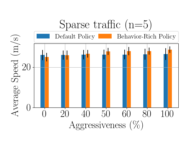
(c) Average speed for $n=5$ vehicles.

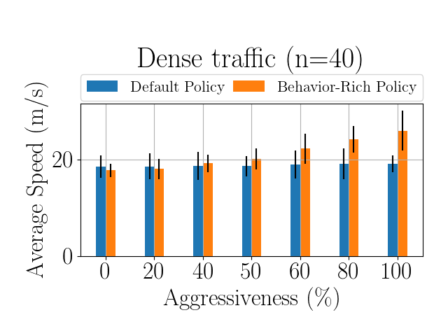
(d) Average speed for $n=40$ vehicles.

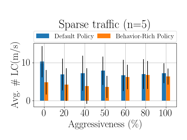
(e) Average number of lane changes for $n=5$ vehicles.

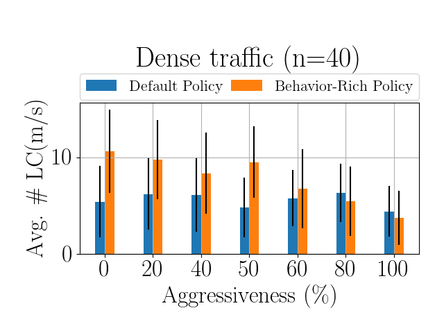
(f) Average number of lane changes for $n=40$ vehicles.

Figure 4: Evaluation: The behavior-rich policy is compared with the default policy in traffic scenarios of varying densities and driver behaviors. The behavior-rich policy leads to improved navigation and a reduced number of collisions (Figures 4(a), 4(b)) by adjusting the speed (Figures 4(c), 4(d)) of the ego-vehicle to the behaviors of its neighbors (higher average speed for higher percentages of aggressive neighbors) and its lane changes (Figures 4(e), 4(f)). When $n=5$ (Figure 4(e)), the number of lane changes increases as the ego-vehicle is more confident in performing lane-changing maneuvers due to the sparsity of the traffic. In contrast, the ego-vehicle performs less lane changes in the dense traffic scenario as the percentage of aggressiveness increases, respecting unpredictable surrounding drivers.

VI Experiments and Results

VI-A Simulator

We used the OpenAI gym-based highway-env simulator [17] and enriched it with various driving behaviors using CMetric [14] (as shown in Figure 2). Our approach is easily transferable to other state-of-the-art simulators [19, 20]. More specifically, the parameters from the underlying motion models we are using [51, 52] are widely used in these simulators. Consequently, CMetric is used to tune these parameters, which can then be used in any of these simulators. In our benchmarks, we consider dense traffic scenarios on a four-lane (lane width = $4m$), one-way highway environment populated by vehicles with various driving behaviors. The ego-vehicle always navigates in the middle of its current lane and can reach speeds ranging from 10 $m/s$ to 30 $m/s$.

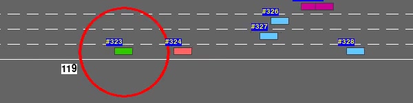
(a) Ego-vehicle approaches aggressive vehicle.

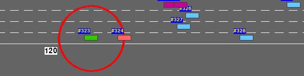
(b) Ego-vehicle slows down.

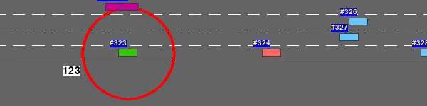
(c) Ego-vehicle slowly accelerates.

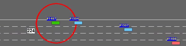
(d) Ego-vehicle approaches conservative vehicle.

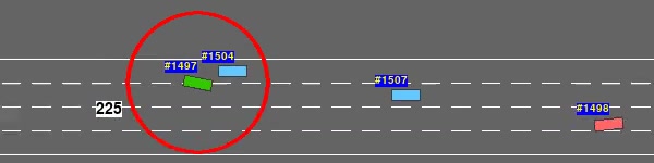
(e) Ego-vehicle switches to adjacent lane.

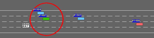
(f) Ego-vehicle overtakes conservative vehicle.

Figure 5: Behavior-Guided Navigation: Interaction with aggressive (top) and conservative (bottom) vehicles. We indicate the ego-vehicle, aggressive vehicles, and conservative vehicles with green, red, and blue colors, respectively. (Top) The ego-vehicle senses that the red vehicle is aggressive and therefore decides to slow down instead of overtaking. (Bottom) The ego-vehicle notices the conservative vehicle in front and decides to confidently overtake it. Our approach can automatically generate such trajectories for the ego-vehicle.

VI-B Implementation and Reward Tuning

We use the PyTorch-based Deep Q Learning implementation [53] to train a $3$-layer MLP model for $3000$ episodes (episode duration=$60$ seconds) in order to tune the reward values using the Epsilon Greedy policy. We initially set $\epsilon=1$ with $0.05$ decay and train using the Adam optimizer with a learning rate of $\eta=0.0005$ and the Mean Squared Error (MSE) loss function. We save the reward values for every $50$ episodes and test the model for $20$ episodes. To avoid sampling correlated samples during the training of the Deep Q network agent, we use Prioritized Experience Replay [54]. The MLP model receives as input a feature matrix that includes the features for each vehicle present in the current simulation. The simulator provides an observation from the environment in the form of an $F\times V$ matrix, where $V$ is the number of vehicles in the simulation and $F$ is the number of features that constitutes the state space of each vehicle.

Our goal is to achieve a low collision frequency while simultaneously maintaining the speed of the ego-vehicle at levels that guarantee efficient navigation and smooth traffic flow. We manually tune the reward values monitoring the collision frequency and the average speed of the ego-vehicle at test time. The same reward values are used for all types of traffic considered. We increase the reward value $r_{HS}$ when the ego-vehicle is moving too slowly and decrease the reward for collisions $r_{C}$, thereby penalizing collisions, when the ego-vehicle is prioritizing higher speed over collision avoidance. We also keep the value of $r_{RL}$ at a low level so that the ego-vehicle does not stay too long in the right lane. Furthermore, we tune $r_{LC}$ based on the pattern, according to which the ego-vehicle performs a lane change. More specifically, we visually inspect the performance at test time and increase $r_{LC}$ when the ego-vehicle tends to stay too long behind other vehicles while the adjacent lanes are empty to encourage overtaking maneuvers. In contrast, we decrease $r_{LC}$ when the ego-vehicle performs many "unnecessary" lane changes, since they disrupt the smoothness of the generated trajectory and increase the possibility of an accident.

VI-C Evaluation and Results

We evaluate the performance of our method in both sparse and dense traffic scenarios by varying the number of aggressive and conservative agents. We apply three metrics for evaluation averaged over multiple $100$-episode runs:

• Collision frequency (%) of the ego-vehicle measured as a percentage over the total test runs.

• Average speed ($m/s$) of the ego-vehicle, as it captures distance per second covered in a varying time interval.

• Number of lane changes performed by the ego-vehicle on average during the given duration.

In terms of density, we consider a sparse traffic scenario ($n=5$) and a dense traffic scenario ($n=40$). In terms of driver behaviors, we examine seven distinct types of traffic consisting of {$0\%$, $20\%$, $40\%$, $50\%$, $60\%$, $80\%$, $100\%$} aggressive drivers. The remaining drivers in each scenario are conservative agents. For example, in the second scenario, we consider $20\%$ aggressive agents and $80\%$ conservative agents. Figure 4 shows the performance of our behavior-rich policy compared to the default policy generated by the simulator, which does not consider driver behavior. The default policy was trained using an identical training routine in a simulator environment where all the cars follow a default built-in behavior based on the IDM model [51]. In these experiments, the vehicles are observable if they are within $d=180m$ from the ego-vehicle.

In both the sparse (Figure 4(a)) and the dense (Figure 4(b)) scenario, our behavior-rich policy leads to a significantly lower collision rate than the baseline policy of the simulator. We observe fewer collisions when all the road-agents are either aggressive ($100\%$ Aggressiveness) or conservative ($0\%$ Aggressiveness) than when the traffic is mixed ($20\%,40\%,60\%,80\%$ Aggressiveness). This occurs because the ego-vehicle gets confused by the combination of slow-moving vehicles and aggressive agents. To further improve performance, we would need a different set of rewards to be tuned for each specific type of traffic examined. The default policy has a lower collision frequency when the behaviors are aggressive, both in the sparse scenario (Figure 4(a)) and in the dense scenario (Figure 4(b)). This occurs because the ego-vehicle, using the default policy, drives with reduced speed, compared to the aggressive vehicles that overspeed and drive ahead. This creates an empty space around the ego-vehicle as it is “left behind” and reduces the collision frequency compared to the mixed and conservative traffic scenarios when there are vehicles around the ego-vehicle driving at comparable speed.

The average speed of the ego-vehicle increases (Figures 4(c), 4(d)) as the traffic ranges from conservative to aggressive with our behavior-rich policy, as slow-moving conservative vehicles tend to slow the ego-vehicle down. In contrast, the speed in the default policy remains almost unchanged, indicating that the ego-vehicle is unable to adjust to the behaviors of the road-agents and maintains a uniform behavior. Finally, the number of lane changes performed by the ego-vehicle increases as the traffic becomes more aggressive for the sparse traffic scenario (Figure 4(e)) and the behavior-rich policy. In that case, the ego-vehicle leverages the sparsity of the traffic and, influenced by its aggressive neighbors, attempts lane-changing maneuvers more confidently. In the dense traffic scenario (Figure 4(f)), the number of lane changes of the ego-vehicle decreases as the surrounding agents become more aggressive. We show qualitative results in Figure 5.

In addition to the initial experiments that consider a perception radius of $d_{1}=180m$ around the ego-vehicle, we present results (Figure 6) using our behavior-rich simulation technique for limited sensing abilities corresponding to radii of $d_{2}=90m$ and $d_{3}=30m$, respectively. The results show that the navigation performance drops as the perception radius decreases, especially for the dense traffic scenario 6(b), where the ego-vehicle has to deal with a larger number of agents. In summary, our new simulation technique combined with this DRL-based navigation scheme offers the following benefits:

• Increased Safety: Our behavior-rich policy results in a significantly lower collision frequency than the default policy baseline.

• Behavior-Aware Trajectories: Our behavior-rich policy generates behavior-aware trajectories. The ego-vehicle learns to adjust its behavior based on the behavior of its neighbors, both in terms of speed regulation and the number of executed lane changes.

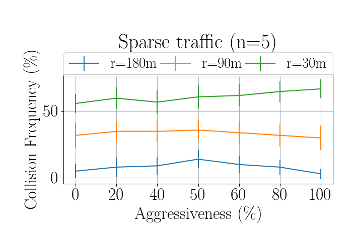
(a) Collision frequency for different ego-perception abilities in sparse traffic.

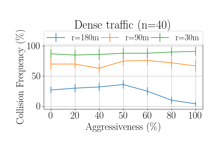
(b) Collision frequency for different ego-perception abilities in dense traffic.

Figure 6: Partial Observability: We model partial observability by reducing the perception ability of the ego-vehicle, adding vehicles to the state space only when they are within a specified radius from the ego-vehicle. We present results in terms of collisions from experiments that follow a behavior-rich policy and consider a perception radius around $180m$, $90m$, and $30m$ from the ego-vehicle. The navigation performance drops as the radius decreases and the number of crashes is larger when the ego-vehicle has to navigate around a larger number of agents (Figure 6(b)).

VII Conclusion, Limitations, and Future Work

We proposed a new simulation technique for enriching traffic simulators with behavior-rich trajectories corresponding to varying levels of aggressiveness. Based on this technique, we presented a navigation scheme that is based on deep reinforcement learning and considers driver behavior to perform behaviorally-guided navigation. Our preliminary results in many benchmarks are encouraging and our approach can handle scenarios with high traffic density and aggressive behaviors. Our behavior generation module can be easily transferred to any state-of-the-art parametric traffic simulator and can generate synthetic traffic datasets consisting of realistic behavior-rich trajectories, which can provide fruitful and diverse training scenarios to state-of-the-art data-driven approaches.

Our method has several limitations. For example, in some cases, the ego-vehicle avoids aggressive vehicles by decelerating and performing fewer lane changes, thereby acting conservatively. In some scenarios, it may be necessary to execute non-conservative actions such as increasing the frequency of lane changes or following local traffic norms. Furthermore, the performance of our approach drops as the perception radius of the ego-vehicle decreases, which means that it would require very good sensing for it to be applicable to real-world scenarios. In terms of future work, we plan to extend our approach to different environments like roundabouts, intersections, and parking lots and perform more detailed evaluation. Furthermore, we plan to develop efficient navigation techniques to handle heterogeneous traffic-agents such as pedestrians or bicycles.

Appendix A CMetric: Mapping Trajectories to Behavior

A-A Centrality Measures

In graph theory and network analysis, centrality measures [48] are real-valued functions $\zeta:\mathcal{V}\longrightarrow\mathbb{R}$, where $\mathcal{V}$ denotes the set of vertices and $\mathbb{R}$ denotes a scalar real number that identifies key vertices within a graph network. So far, centrality functions have been restricted to identifying influential personalities in online social media networks [55] and key infrastructure nodes in the Internet [56], to rank web-pages in search engines [57], and to discover the origin of epidemics [58]. There are several types of centrality functions. The ones that are of particular importance to us are the degree centrality and the closeness centrality denoted as $\zeta_{d}(t)$ and $\zeta_{c}(t)$, respectively. These centrality measures are defined in [14] (See section III-C). Each function measures a different property of a vertex. Typically, the choice of selecting a centrality function depends on the current application at hand. In this work, the closeness centrality and the degree centrality functions measure the likelihood and intensity of specific driving styles such as overspeeding, overtaking, sudden lane-changes, and weaving [14].

A-B Algorithm

Here, we present the main algorithm, called CMetric. CMetric maps vehicle trajectories to specific styles by computing the likelihood and intensity of the latter using the definitions of the centrality functions. The specific styles are then used to assign global behaviors [33]. We summarize the CMetric algorithm as follows:

1. Obtain the positions of all vehicles using localization sensors deployed on the autonomous vehicle and form traffic-graphs at each time-step.

2. Compute the closeness and degree centrality function values for each vehicle at every time-step.

3. Perform polynomial regression to generate uni-variate polynomials of the centralities as a function of time.

4. Measure likelihood and intensity of a specific style for each vehicle by analyzing the first- and second-order derivatives of their centrality polynomials.

We begin by forming the traffic-graphs for each frame and use the definitions in [14] to compute the discrete-valued centrality measures. Since centrality measures are discrete functions, we perform polynomial regression using regularized Ordinary Least Squares (OLS) solvers to transform the two centrality functions into continuous polynomials, $\zeta_{c}(t)$ and $\zeta_{d}(t)$, as a function of time. We describe polynomial regression in detail in the following subsections. We compute the likelihood and intensity of specific styles by analyzing the first- and second-order derivatives of $\zeta_{c}(t)$ and $\zeta_{d}(t)$.

A-C Polynomial Regression

In order to study the behavior of the centrality functions with respect to how they change with time, we convert the discrete-valued $\zeta[t]$ into continuous-valued polynomials $\zeta(t)$, using which we calculate the first- and second-order derivatives of the centrality functions as explained in Section A-D.

In this work, we choose a quadratic centrality polynomial can be expressed as $\zeta(t)=\beta_{0}+\beta_{1}t+\beta_{2}t^{2}$, as a function of time. Here, $\beta=[\beta_{0}\ \beta_{1}\ \beta_{2}]^{\top}$ are the polynomial coefficients. These coefficients can be computed using ordinary least squares (OLS) equation as follows,

$$\beta=(M^{\top}M)\raisebox{4.52083pt}{$\scriptscriptstyle-\!1$}M^{\top}\zeta^{i}$$ (2)

Here, $M\in\mathbb{R}^{T\times(d+1)}$ is the Vandermonde matrix [59]. and is given by,

$$M=\begin{bmatrix}1&t_{1}&t^{2}_{1}&\dots&t^{d}_{1}\\ 1&t_{2}&t^{2}_{2}&\dots&t^{d}_{2}\\ \vdots&\vdots&\vdots&\ddots&\vdots\\ 1&t_{T}&t^{2}_{T}&\dots&t^{d}_{T}\end{bmatrix}$$

A-D Style Likelihood and Intensity Estimates

In the previous sections, we used polynomial regression on the centrality functions to compute centrality polynomials. In this section, we analyze and discuss the first and second derivatives of the degree centrality, $\zeta_{d}(t)$, and closeness centrality, $\zeta_{c}(t)$, polynomials. Based on this analysis, which may vary for each specific style, we compute the Style Likelihood Estimate (SLE) and Style Intensity Estimate (SIE) [14], which are used to measure the probability and the intensity of a specific style.

Overtaking/Sudden Lane-Changes

Overtaking is when one vehicle drives past another vehicle in the same or an adjacent lane, but in the same direction. The closeness centrality increases as the vehicle navigates towards the center and vice-versa. The SLE of overtaking can be computed by measuring the first derivative of the closeness centrality polynomial using $\textrm{SLE}(t)=\left\lvert\frac{\partial\zeta_{c}(t)}{\partial t}\right\rvert$. The maximum likelihood $\textrm{SLE}_{\textrm{max}}$ can be computed as $\textrm{SLE}_{\textrm{max}}=\max_{t\in\Delta t}{\textrm{SLE}}(t)$. The SIE of overtaking is computed by simply measuring the second derivative of the closeness centrality using $\textrm{SIE}(t)=\left\lvert\frac{\partial^{2}\zeta_{c}(t)}{\partial t^{2}}\right\rvert$. Sudden lane-changes follow a similar maneuver to overtaking and therefore can be modeled using the same equations used to model overtaking.

Overspeeding

The degree centrality can be used to model overspeeding. As $A_{t}$ is formed by adding rows and columns to $A_{t-1}$, the degree of the $i^{\textrm{th}}$ vehicle (denoted as $\theta_{i}$) is calculated by simply counting the number of non-zero entries in the $i^{\textrm{th}}$ row of $A_{t}$. Intuitively, a drivers that are overspeeding will observe new neighbors along the way (increasing degree) at a higher rate than conservative, or even neutral, drivers. Let the rate of increase of $\theta_{i}$ be denoted as $\theta_{i}^{{}^{\prime}}$. By definition of the degree centrality and construction of $A_{t}$, the degree centrality for an aggressively overspeeding vehicle will monotonically increase. Conversely, the degree centrality for a conservative vehicle driving at a uniform speed or braking often at unconventional spots such as green light intersections will be relatively flat. Therefore, the likelihood of overspeeding can be measured by computing,

$$\textrm{SLE}(t)=\left\lvert\frac{\partial\zeta_{d}(t)}{\partial t}\right\rvert$$

Similar to overtaking, the maximum likelihood estimate is given by $\textrm{SLE}_{\textrm{max}}=\max_{t\in\Delta t}{\textrm{SLE}}(t)$.

Weaving

A vehicle is said to be weaving when it “zig-zags” through traffic. Weaving is characterized by oscillation in the closeness centrality values between low values towards the sides of the road and high values in the center. Mathematically, weaving is more likely to occur near the critical points (points at which the function has a local minimum or maximum) of the closeness centrality polynomial. The critical points $t_{c}$ belong to the set $\mathcal{T}=\big{\{}t_{c}\big{|}\frac{\partial\zeta_{c}(t_{c})}{\partial t}=0\big{\}}$. Note that $\mathcal{T}$ also includes time-instances corresponding to the domain of constant functions that characterize conservative behavior. We disregard these points by restricting the set membership of $\mathcal{T}$ to only include those points $t_{c}$ whose $\varepsilon-$sharpness [60] of the closeness centrality is non-zero. The set $\mathcal{T}$ is reformulated as follows,

$$\mathcal{T}=\Bigg{\{}t_{c}\bigg{|}\frac{\partial\zeta_{c}(t_{c})}{\partial t}=0\Bigg{\}}$$ (3)

$$\textrm{s.t.}\max_{t\in\mathcal{B}_{\varepsilon}(t_{c})}\frac{\partial\zeta_{c}(t)}{\partial t}\neq\frac{\partial\zeta_{c}(t_{c})}{\partial t}$$

where $\mathcal{B}_{\varepsilon}(y)\in\mathbb{R}^{d}$ is the unit ball centered around a point $y$ with radius $\varepsilon$. The SLE of a weaving vehicle is represented by $\lvert\mathcal{T}\rvert$, which represents the number of elements in $\mathcal{T}$. The $\textrm{SIE}(t)$ is computed by measuring the $\varepsilon-$sharpness value of each $t_{c}\in\mathcal{T}$.

Conservative Vehicles

Conservative vehicles, on the other hand, are not inclined towards aggressive maneuvers such as sudden lane-changes, overspeeding, or weaving. Rather, they tend to stick to a single lane [61] as much as possible, and drive at a uniform speed [33] below the speed limit. Correspondingly, the values of the closeness and degree centrality functions in the case of conservative vehicles remain constant. Mathematically, the first derivative of constant polynomials is $0$. The SLE of conservative behavior is therefore observed to be approximately equal to $0$. Additionally, the likelihood that a vehicle drives uniformly in a single lane during time-period $\Delta t$ is higher when,

$$\left\lvert\frac{\partial\zeta_{c}(t)}{\partial t}\right\rvert\approx 0\ \textrm{and}\ \max_{t\in\mathcal{B}_{\varepsilon}(t^{*})}\textrm{SLE}(t)\approx\textrm{SLE}(t_{c}).$$

The intensity of such maneuvers will be low and is reflected in the lower values for the SIE.

TABLE II: Comparison with Prior Work: We compare B-GAP with prior DRL-based navigation methods. For fair comparison, we compare % collisions along with the number of vehicles and the number of episodes used for training.

Methods	# vehicles	# episodes	% collisions
DDPG [2]	$4$	$4000$	$10.13$
PS-DDPG [1]	$5$	$600$	$11.40$
B-GAP	$5$	$3000$	3.00

A-E Comparison with DRL-Based Navigation Methods

We compare our navigation scheme with state-of-the-art DRL-based methods that train navigation policies in highway environments consisting of $4-5$ vehicles, with a maximum density of $5$ vehicles. However, these methods do not consider aggressive agents and have not been tested in complex scenarios with high numbers of vehicles and varying behaviors, as we have evaluated (with $n=40$) in Figure 4. Our navigation method results in very few collisions in high density scenarios ($n=40$ as compared to maximum $5$ used in [1]) with aggressive agents (Figure 4).

In Table II, we compare our approach with these methods in terms of % collisions. For fair comparison, we use $n=5$ in the aggressive environment since prior methods [2, 1] have also tested with $4-5$ vehicles, respectively. We also include the number of vehicles and training episodes since the performance of these methods depends on them. It should be noted that these approaches use a continuous action space, while we use a discrete action space.

References

- [1] M. Kaushik, K. M. Krishna et al., “Parameter sharing reinforcement learning architecture for multi agent driving behaviors,” arXiv preprint arXiv:1811.07214, 2018.
- [2] M. Kaushik, V. Prasad, K. M. Krishna, and B. Ravindran, “Overtaking maneuvers in simulated highway driving using deep reinforcement learning,” in 2018 ieee intelligent vehicles symposium (iv). IEEE, 2018, pp. 1885–1890.
- [3] H. Song, W. Ding, Y. Chen, S. Shen, M. Y. Wang, and Q. Chen, “PiP: Planning-Informed Trajectory Prediction for Autonomous Driving,” Lecture Notes in Computer Science, p. 598–614, 2020. [Online]. Available: http://dx.doi.org/10.1007/978-3-030-58589-1_36
- [4] N. Deo and M. M. Trivedi, “Multi-Modal Trajectory Prediction of Surrounding Vehicles with Maneuver based LSTMs,” 2018 IEEE Intelligent Vehicles Symposium (IV), Jun 2018. [Online]. Available: http://dx.doi.org/10.1109/IVS.2018.8500493
- [5] D. Tesla, “25 Miles of Full Self Driving, TESLA CHALLENGE 2, Autopilot,” https://www.youtube.com/watch?v=Rm8aPR0aMDE, 2019.
- [6] R. Chandra, M. Mahajan, R. Kala, R. Palugulla, C. Naidu, A. Jain, and D. Manocha, “Meteor: A massive dense & heterogeneous behavior dataset for autonomous driving,” arXiv preprint arXiv:2109.07648, 2021.
- [7] A. Davies, “Google’s self-driving car caused its first crash,” 2016.
- [8] S. Anthony, “Self-driving cars still can’t mimic the most natural human behavior,” https://qz.com/1064004/self-driving-cars-still-cant-mimic-the-most-natural-human-behavior/, 2017.
- [9] W. Schwarting, A. Pierson, J. Alonso-Mora, S. Karaman, and D. Rus, “Social behavior for autonomous vehicles,” Proceedings of the National Academy of Sciences, vol. 116, no. 50, pp. 24 972–24 978, 2019.
- [10] A. Doshi and M. M. Trivedi, “Examining the impact of driving style on the predictability and responsiveness of the driver: Real-world and simulator analysis,” in 2010 IEEE Intelligent Vehicles Symposium. IEEE, 2010, pp. 232–237.
- [11] A. Corti, C. Ongini, M. Tanelli, and S. M. Savaresi, “Quantitative driving style estimation for energy-oriented applications in road vehicles,” in 2013 IEEE International Conference on Systems, Man, and Cybernetics. IEEE, 2013, pp. 3710–3715.
- [12] J. Rong, K. Mao, and J. Ma, “Effects of individual differences on driving behavior and traffic flow characteristics,” Transportation research record, vol. 2248, no. 1, pp. 1–9, 2011.
- [13] K. H. Beck, B. Ali, and S. B. Daughters, “Distress tolerance as a predictor of risky and aggressive driving.” Traffic injury prevention, vol. 15 4, pp. 349–54, 2014.
- [14] R. Chandra, U. Bhattacharya, T. Mittal, A. Bera, and D. Manocha, “CMetric: A Driving Behavior Measure Using Centrality Functions,” arXiv preprint arXiv:2003.04424, 2020.
- [15] R. Chandra, T. Guan, S. Panuganti, T. Mittal, U. Bhattacharya, A. Bera, and D. Manocha, “Forecasting trajectory and behavior of road-agents using spectral clustering in graph-lstms,” IEEE Robotics and Automation Letters, 2020.
- [16] C. Li, Y. Meng, S. H. Chan, and Y.-T. Chen, “Learning 3D-aware Egocentric Spatial-Temporal Interaction via Graph Convolutional Networks,” arXiv preprint arXiv:1909.09272, 2019.
- [17] E. Leurent, “An Environment for Autonomous Driving Decision-Making,” https://github.com/eleurent/highway-env, 2018.
- [18] V. Mnih, K. Kavukcuoglu, D. Silver, A. A. Rusu, J. Veness, M. G. Bellemare, A. Graves, M. Riedmiller, A. K. Fidjeland, G. Ostrovski et al., “Human-level control through deep reinforcement learning,” nature, vol. 518, no. 7540, pp. 529–533, 2015.
- [19] P. A. Lopez, M. Behrisch, L. Bieker-Walz, J. Erdmann, Y.-P. Flötteröd, R. Hilbrich, L. Lücken, J. Rummel, P. Wagner, and E. Wießner, “Microscopic Traffic Simulation using SUMO,” in The 21st IEEE International Conference on Intelligent Transportation Systems. IEEE, 2018. [Online]. Available: https://elib.dlr.de/124092/
- [20] A. Dosovitskiy, G. Ros, F. Codevilla, A. Lopez, and V. Koltun, “CARLA: An Open Urban Driving Simulator,” 2017.
- [21] A. De Luca, G. Oriolo, and C. Samson, “Feedback control of a nonholonomic car-like robot,” in Robot motion planning and control. Springer, 1998, pp. 171–253.
- [22] S. M. LaValle and J. J. Kuffner Jr, “Randomized kinodynamic planning,” The international journal of robotics research, vol. 20, no. 5, pp. 378–400, 2001.
- [23] A. Liniger, A. Domahidi, and M. Morari, “Optimization-based autonomous racing of 1: 43 scale RC cars,” Optimal Control Applications and Methods, vol. 36, no. 5, pp. 628–647, 2015.
- [24] J. Roh, C. I. Mavrogiannis, R. Madan, D. Fox, and S. S. Srinivasa, “Multimodal Trajectory Prediction via Topological Invariance for Navigation at Uncontrolled Intersections,” CoRR, vol. abs/2011.03894, 2020. [Online]. Available: https://arxiv.org/abs/2011.03894
- [25] Y. F. Chen, M. Everett, M. Liu, and J. P. How, “Socially aware motion planning with deep reinforcement learning,” in 2017 IEEE/RSJ International Conference on Intelligent Robots and Systems (IROS). IEEE, 2017, pp. 1343–1350.
- [26] C. Chen, Y. Liu, S. Kreiss, and A. Alahi, “Crowd-Robot Interaction: Crowd-aware Robot Navigation with Attention-based Deep Reinforcement Learning,” arXiv preprint arXiv:1809.08835, 2018.
- [27] R. Chandra, U. Bhattacharya, A. Bera, and D. Manocha, “Traphic: Trajectory prediction in dense and heterogeneous traffic using weighted interactions,” in Proceedings of the IEEE Conference on Computer Vision and Pattern Recognition, 2019, pp. 8483–8492.
- [28] R. Chandra, U. Bhattacharya, C. Roncal, A. Bera, and D. Manocha, “Robusttp: End-to-end trajectory prediction for heterogeneous road-agents in dense traffic with noisy sensor inputs,” in ACM Computer Science in Cars Symposium, 2019, pp. 1–9.
- [29] I. J. Goodfellow, J. Shlens, and C. Szegedy, “Explaining and harnessing adversarial examples,” arXiv preprint arXiv:1412.6572, 2014.
- [30] E. R. Dahlen, B. D. Edwards, T. Tubré, M. J. Zyphur, and C. R. Warren, “Taking a look behind the wheel: An investigation into the personality predictors of aggressive driving,” Accident Analysis & Prevention, vol. 45, pp. 1–9, 2012.
- [31] A. H. Jamson, N. Merat, O. M. Carsten, and F. C. Lai, “Behavioural changes in drivers experiencing highly-automated vehicle control in varying traffic conditions,” Transportation research part C: emerging technologies, vol. 30, pp. 116–125, 2013.
- [32] P. Jackson, C. Hilditch, A. Holmes, N. Reed, N. Merat, and L. Smith, “Fatigue and road safety: a critical analysis of recent evidence,” Department for Transport, Road Safety Web Publication, vol. 21, 2011.
- [33] F. Sagberg, Selpi, G. F. Bianchi Piccinini, and J. Engström, “A review of research on driving styles and road safety,” Human factors, vol. 57, no. 7, pp. 1248–1275, 2015.
- [34] W. Schwarting, J. Alonso-Mora, and D. Rus, “Planning and decision-making for autonomous vehicles,” Annual Review of Control, Robotics, and Autonomous Systems, 2018.
- [35] N. Li, D. W. Oyler, M. Zhang, Y. Yildiz, I. Kolmanovsky, and A. R. Girard, “Game theoretic modeling of driver and vehicle interactions for verification and validation of autonomous vehicle control systems,” IEEE Transactions on control systems technology, vol. 26, no. 5, pp. 1782–1797, 2017.
- [36] Z. Cao, E. Bıyık, W. Z. Wang, A. Raventos, A. Gaidon, G. Rosman, and D. Sadigh, “Reinforcement Learning based Control of Imitative Policies for Near-Accident Driving,” 2020.
- [37] Z. Constantinescu, C. Marinoiu, and M. Vladoiu, “Driving style analysis using data mining techniques,” International Journal of Computers Communications & Control, vol. 5, no. 5, pp. 654–663, 2010.
- [38] W. Schwarting, A. Pierson, J. Alonso-Mora, S. Karaman, and D. Rus, “Social behavior for autonomous vehicles,” Proceedings of the National Academy of Sciences, vol. 116, no. 50, pp. 24 972–24 978, 2019.
- [39] D. Sadigh, S. Sastry, S. A. Seshia, and A. D. Dragan, “Planning for autonomous cars that leverage effects on human actions.” in Robotics: Science and Systems, vol. 2. Ann Arbor, MI, USA, 2016.
- [40] A. Kuefler, J. Morton, T. Wheeler, and M. Kochenderfer, “Imitating driver behavior with generative adversarial networks,” in 2017 IEEE Intelligent Vehicles Symposium (IV). IEEE, 2017, pp. 204–211.
- [41] R. Chandra, A. Bera, and D. Manocha, “Using graph-theoretic machine learning to predict human driver behavior,” IEEE Transactions on Intelligent Transportation Systems, 2021.
- [42] R. Chandra, U. Bhattacharya, T. Mittal, X. Li, A. Bera, and D. Manocha, “GraphRQI: Classifying Driver Behaviors Using Graph Spectrums,” arXiv preprint arXiv:1910.00049., 2019.
- [43] R. Chandra, A. Bera, and D. Manocha, “Stylepredict: Machine theory of mind for human driver behavior from trajectories,” arXiv preprint arXiv:2011.04816, 2020.
- [44] H. Zhao, A. Cui, S. A. Cullen, B. Paden, M. Laskey, and K. Goldberg, “FLUIDS: A First-Order Lightweight Urban Intersection Driving Simulator,” in 2018 IEEE 14th International Conference on Automation Science and Engineering (CASE), 2018, pp. 697–704.
- [45] W. Li, C. Pan, R. Zhang, J. Ren, Y. Ma, J. Fang, F. Yan, Q. Geng, X. Huang, H. Gong et al., “Aads: Augmented autonomous driving simulation using data-driven algorithms,” Science robotics, vol. 4, no. 28, 2019.
- [46] S. Suo, S. Regalado, S. Casas, and R. Urtasun, “TrafficSim: Learning to Simulate Realistic Multi-Agent Behaviors,” 2021.
- [47] S. Shiroshita, S. Maruyama, D. Nishiyama, M. Y. Castro, K. Hamzaoui, G. Rosman, J. DeCastro, K.-H. Lee, and A. Gaidon, “Behaviorally Diverse Traffic Simulation via Reinforcement Learning,” 2020.
- [48] F. A. Rodrigues, “Network Centrality: An Introduction,” A Mathematical Modeling Approach from Nonlinear Dynamics to Complex Systems, p. 177, 2019.
- [49] E. Leurent and J. Mercat, “Social Attention for Autonomous Decision-Making in Dense Traffic,” arXiv preprint arXiv:1911.12250, 2019.
- [50] A. Mavrogiannis, R. Chandra, and D. Manocha, “B-GAP: Behavior-Rich Simulation and Navigation for Autonomous Driving,” arXiv preprint arXiv:2011.03748, 2021.
- [51] M. Treiber, A. Hennecke, and D. Helbing, “Congested traffic states in empirical observations and microscopic simulations,” Physical review E, vol. 62, no. 2, p. 1805, 2000.
- [52] A. Kesting, M. Treiber, and D. Helbing, “General lane-changing model MOBIL for car-following models,” Transportation Research Record, vol. 1999, no. 1, pp. 86–94, 2007.
- [53] E. Leurent, “rl-agents: Implementations of Reinforcement Learning algorithms,” https://github.com/eleurent/rl-agents, 2018.
- [54] T. Schaul, J. Quan, I. Antonoglou, and D. Silver, “Prioritized Experience Replay,” 2016.
- [55] S. A. Morelli, D. C. Ong, R. Makati, M. O. Jackson, and J. Zaki, “Empathy and well-being correlate with centrality in different social networks,” Proceedings of the National Academy of Sciences, vol. 114, no. 37, pp. 9843–9847, 2017.
- [56] G. Lawyer, “Understanding the influence of all nodes in a network,” Scientific reports, vol. 5, no. 1, pp. 1–9, 2015.
- [57] L. Page, S. Brin, R. Motwani, and T. Winograd, “The pagerank citation ranking: Bringing order to the web.” Stanford InfoLab, Tech. Rep., 1999.
- [58] M. Šikić, A. Lančić, N. Antulov-Fantulin, and H. Štefančić, “Epidemic centrality is there an underestimated epidemic impact of network peripheral nodes?” The European Physical Journal B, vol. 86, no. 10, p. 440, 2013.
- [59] D. Manocha, Algebraic and numeric techniques in modeling and robotics. University of California at Berkeley, 1992.
- [60] L. Dinh, R. Pascanu, S. Bengio, and Y. Bengio, “Sharp minima can generalize for deep nets,” in Proceedings of the 34th International Conference on Machine Learning-Volume 70. JMLR. org, 2017, pp. 1019–1028.
- [61] K. I. Ahmed, “Modeling drivers’ acceleration and lane changing behavior,” Ph.D. dissertation, MIT, 1999.