Projectively topological exceptional points in non-Hermitian Rice-Mele model

Abstract

We study coupled non-Hermitian Rice-Mele chains, which consist of Su-Schrieffer-Heeger (SSH) chain system with staggered on-site imaginary potentials. In two dimensional ($2$D) thermodynamic limit, the exceptional points (EPs) are shown to exhibit topological feature: EPs correspond to topological defects of a real auxiliary $2$D vector field in $\boldsymbol{k}$ space, which is obtained from the Bloch states of the non-Hermitian Hamiltonian. As a topological invariant, the topological charges of EPs can be $\pm 1/2$, obtained by the winding number calculation. Remarkably, we find that such a topological characterization remains for a finite number of coupled chains, even a single chain, in which the momentum in one direction is discrete. It shows that the EPs in the quasi-$1$D system still exhibit topological characteristics and can be an abridged version for a $2$D system with symmetry protected EPs that are robust in perturbations, which proves that topological invariants for a quasi-$1$D system can be extracted from the projection of the corresponding $2$D limit system on it.

I Introduction

Exceptional point (EP) is an exclusive critical point in non-Hermitian systems, at which many exotic features occur Bender ; Longhi ; West ; LC ; Yang ; Zhang ; Longhi1 ; Goldzak ; Yi . It is also called non-Hermitian degeneracy or branch point in the complex energy plane, where two eigenvalues and their eigenvectors become the same, referred to as a coalescing level Heiss . Mathematically, the occurrence of an EP relates to the emergence of a Jordan block. Two eigenvectors of a $2\times 2$ Jordan block are the same and self-orthogonal Ali1 . Unlike the level crossing in the Hermitian matrix around the degenerate point, there is a level repulsion near the EP. In general, EPs are sensitive to the parameters of the system. In a continuous system with translational symmetry, the eigen problem is reduced to that of a small non-Hermitian system, where momentum $k$ acts as a system parameter Ali2 .

With these unusual properties, recently there have been growing efforts to investigate topological phenomena of non-Hermitian systems, both theoretically Esaki ; Tony ; Li1 ; Lin ; Nori ; Fu ; Yao ; Gong and experimentally Ding ; Dop ; Weim ; Feng . Compared with Hermitian systems, of which degenerate points play an important role in topological properties Niu ; Kane ; ZhangSQ ; Burkov ; Xu ; Young ; Sama ; Weng ; Huang ; Hou ; Liu ; Neupane ; SXu ; Lv ; Lu , no effective method such as the calculation of the winding number or Chern number in Hermitian systems Niu ; Kane ; ZhangSQ is established to describe the topological feature of EPs. Based on this, Almost all theoretical works try to define or find a group of new topological invariant to distinguish the phase diagram of non-Hermitian systems, some of them are applicable for families of non-Hermitian Hamiltonians Esaki ; Nori ; Fu ; Gong , others focus on the specific model Tony ; Li1 ; Lin ; Yao . Therefore, the description of the topological feature of EPs remains an open question.

In this work, we study $M$ coupled non-Hermitian Rice-Mele chains with length $2N$ RM ; Lin1 ; WR . The non-Hermiticity arises from staggered on-site imaginary potentials on the Hermitian coupled Su-Schrieffer-Heeger (SSH) chains SSH ; As . The exact solution shows that the EPs can be two isolated points in two dimensional ($2$D) $\boldsymbol{k}$-plane for infinite $M$ and $N$, or $2$D thermodynamic limit. When parameters of the system vary, such two points move in the plane and cannot be removed until they meet together. We map the Bloch states of the non-Hermitian Hamiltonian onto a $2$D real vector field in $\boldsymbol{k}$-plane, referred to as an auxiliary field. It is shown that two isolated EPs are topological defects of the field with a topological charge $\pm 1/2$, which exhibits the topological feature of the EPs. Furthermore, we extend this analysis to finite $M$ cases with periodic and open boundary conditions. The distribution of the auxiliary field at a pair of EPs in the systems with even $M$ and periodic boundary condition (or odd $M$ with open boundary condition) reflects the same topological configuration, which indicates that the auxiliary field for finite $M$ on the discrete $\boldsymbol{k}$ space is the projection of the infinite one for the $2$D model. In this sense, the topological charge obtained from the $2$D model in the thermodynamic limit can characterize the EPs for finite $M$, even for $M=1$. Therefore, we focus on the single-chain system and find that two topological defects in $2$D $\boldsymbol{k}$ space reduce to a pair of kinks in $1$D $k$ space. The corresponding topological invariant is protected by the combined inversion and time-reversal symmetry. At last, the behavior of the topological gapless system in the presence of several types of perturbations is performed, which shows the robust topological feature of the EPs in non-Hermitian systems is the same as the band touching points in Hermitian systems.

The remainder of this paper is organized as follows. In Sec. II, we present $M$ coupled non-Hermitian Rice-Mele chains with length $2N$ and its phase diagram. Sec. III reveals the topological feature of nodal points of the $2$D system in the thermodynamic limit and corresponding topological configuration in the finite $2$D system. Sec. IV shows the single-chain solution, including the energy band, eigenvector, and topological properties. Sec. V devotes to the symmetries that protect the topological invariants of the single SSH chain. Sec. VI displays the behavior of the topological gapless system in the presence of several types of perturbations. Finally, we present a summary and discussion in Sec. VII.

II Model and Phase diagram

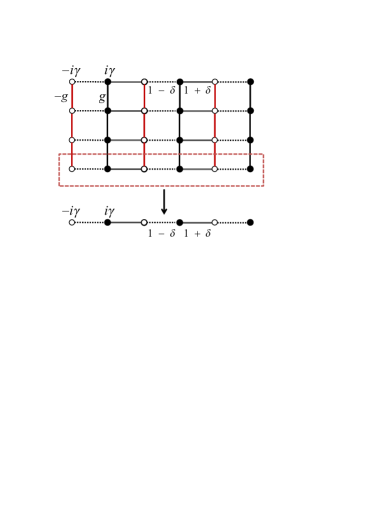
Figure 1: (Color online) Schematics of the simplest bundle of $M$ non-Hermitian dimerized chains with staggered balanced gain and loss. Hopping amplitudes along the $x$ direction are staggered by $1+\delta$ (double line) and $1-\delta$ (dash line). Along the $y$ direction, it is a uniform chain with inter-chain tunneling constant $g$ ($-g$). When the system reduces into the $1$D situation, it can be seen as a SSH chain with on-site imaginary potentials, which will be explored in the rest of the paper.

We consider a bundle of $M$ non-Hermitian dimerized chains with staggered balanced gain and loss, two neighboring of which are coupled. The simplest tight-binding model with these features is

$$H = -J\sum_{l=1}^{2N}\sum_{n=1}^{M}\left[1+\left(-1\right)^{l}\delta\right]\left(c_{l,n}^{\dagger}c_{l+1,n}+\mathrm{H.c.}\right)$$ (1)

$$+g\sum_{l=1}^{2N}\sum_{n=1}^{M}\left(-1\right)^{l}\left(c_{l,n}^{\dagger}c_{l,n+1}+\mathrm{H.c.}\right)$$

$$+i\gamma\sum_{l,n}\left(-1\right)^{l}c_{l,n}^{\dagger}c_{l,n},$$

where $J$, $\delta$, $g$ and $i\gamma$ ($\gamma>0$), as showed in Fig. 1, are the inter-chain hopping strengths, the distortion factor, inter-chain tunneling constant and the alternating imaginary potential magnitude, respectively. Here $c_{l,n}^{\dagger}$ is the creation operator of the fermion at the $l$th site in $n$th chain. The periodic boundary conditions along two directions are imposed as $c_{2N+1,n}=c_{1,n}$ and $c_{l,M+1}=c_{l,1}$. We decompose the system into two sub-lattices $A$ and $B$ and rewrite the Hamiltonian as

$$H = -J\sum_{l=1}^{N}\sum_{n=1}^{M}\left[\left(1-\delta\right)a_{l,n}^{\dagger}b_{l,n}+\left(1+\delta\right)b_{l,n}^{\dagger}a_{l+1,n}+\mathrm{H.c.}\right]$$ (2)

$$-g\sum_{l=1}^{N}\sum_{n=1}^{M}\left(a_{l,n}^{\dagger}a_{l,n+1}-b_{l,n}^{\dagger}b_{l,n+1}+\mathrm{H.c.}\right)$$

$$+i\gamma\sum_{l,n}\left(b_{l,n}^{\dagger}b_{l,n}-a_{l,n}^{\dagger}a_{l,n}\right),$$

where $a_{l}^{{\dagger}}$ and $b_{l}^{{\dagger}}$ are the creation operators of fermion at $l$th site of sub-lattice $A$ and $B$, respectively. Taking the Fourier transformations

$$\left\{\begin{array}[]{c}a_{\boldsymbol{k}}=\frac{1}{\sqrt{NM}}\sum_{l,n}e^{i(k_{x}l+k_{y}n)}a_{l,n}\\ b_{\boldsymbol{k}}=\frac{1}{\sqrt{NM}}\sum_{l,n}e^{i(k_{x}l+k_{y}n)}b_{l,n}\end{array}\right.,$$ (3)

where $\boldsymbol{k}=(k_{x},k_{y})$ $=(2\pi n_{x}/N-\pi,2\pi n_{y}/M-\pi)$, with $n_{x}=0,1,2,\ldots,N-1,n_{y}=0,1,2,\ldots,M-1$, we have

$$H=\sum_{\boldsymbol{k}}H_{\boldsymbol{k}}=\sum_{\boldsymbol{k}}(a_{\boldsymbol{k}}^{\dagger},b_{\boldsymbol{k}}^{\dagger})h_{\boldsymbol{k}}\left(\begin{array}[]{c}a_{\boldsymbol{k}}\\ b_{\boldsymbol{k}}\end{array}\right).$$ (4)

Here we just let $J=1$ for simplicity. The core matrix is

$$h_{\boldsymbol{k}}=-\left(\begin{array}[]{cc}V_{k}+i\gamma&\left(1-\delta\right)+\left(1+\delta\right)e^{-ik_{x}}\\ \left(1-\delta\right)+\left(1+\delta\right)e^{ik_{x}}&-\left(V_{k}+i\gamma\right)\end{array}\right),$$ (5)

where

$$V_{\boldsymbol{k}}=2g\cos k_{y}.$$ (6)

The spectrum is

$$\varepsilon_{k}=\pm 2\sqrt{\left(1-\delta^{2}\right)\cos^{2}\left(\frac{k_{x}}{2}\right)+\delta^{2}+\left(g\cos k_{y}+\frac{i\gamma}{2}\right)^{2}}$$ (7)

with the eigenvector

$$\left|\psi_{k}^{\pm}\right\rangle=\frac{1}{\Omega_{\pm}}\left(\begin{array}[]{c}i\gamma+V_{k}\mp\varepsilon_{k}\\ \left(1-\delta\right)+\left(1+\delta\right)e^{ik_{x}}\end{array}\right),$$ (8)

which are normalized by the Dirac normalization factor

$$\Omega_{\pm} = \left|\varepsilon_{k}\right|^{2}\mp\left(2\gamma\mathrm{Im}\varepsilon_{k}+2V_{\mathbf{k}}\mathrm{Re}\varepsilon_{k}\right)+V_{k}^{2}+\gamma^{2}$$ (9)

$$+\varepsilon_{k}^{2}-\left(V_{k}+i\gamma\right)^{2}.$$

From $\varepsilon_{k}=0$, we have equations

$$\left\{\begin{array}[]{c}\left(1-\delta^{2}\right)\cos^{2}\left(\frac{k_{x}}{2}\right)+\delta^{2}-\left(\frac{\gamma}{2}\right)^{2}=0\\ 2g\cos k_{y}=0\end{array}\right..$$ (10)

In $\boldsymbol{k}$ space the zero energy points are located at $\boldsymbol{k}_{c}=(k_{cx},k_{cy})$:

$$\left\{\begin{array}[]{c}\frac{\left(\frac{\gamma}{2}\right)^{2}-\delta^{2}}{1-\delta^{2}}=\cos^{2}\left(\frac{k_{cx}}{2}\right)\\ k_{cy}=\pm\pi/2\end{array}\right..$$ (11)

The restriction $\left|\cos k_{cx}\right|\leqslant 1$ leads to

$$(\gamma^{2}-4\delta^{2})(\gamma^{2}-4)\leqslant 0,$$ (12)

then the boundaries are

$$\left\{\begin{array}[]{c}\gamma_{c}=\pm 2\delta\\ \gamma_{c}=\pm 2\end{array}\right..$$ (13)

Here we note that the boundary line is independent of $g$, so we set $g=1$ for convenience in the rest of the paper. It can be found that the above boundaries divide the parameter space into three parts when $V_{k}=0$: the broken area (where EPs appear), the real and imagine eigenvalues area (where always have an energy gap), which is displayed in Fig. 2. We will show it more clearly in the discussion of single-chain model below.

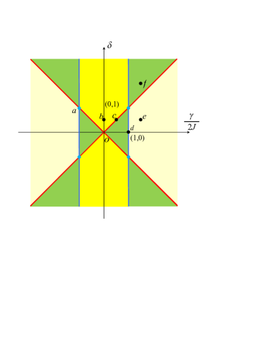
Figure 2: (Color online) Phase diagram of coupled SSH chain system on the $\delta-\gamma/2J$ plane (in the unit of $J$) when $V_{\mathbf{k}}=0$. Red and blue lines indicate the boundary represented in Eq. (13), which separated the area with EPs exist (green), $\varepsilon_{k}$ is real (yellow), and $\varepsilon_{k}$ is imagined (ashen). Four blue circles mean the touching points of two different boundaries.

III Topological nodal points

In this section, we will show that the EPs have topological properties. We demonstrate this point by rewriting the core matrix $h_{\boldsymbol{k}}$ from Eq. (5) in the form

$$h_{\boldsymbol{k}}=\mathbf{B}\left(\boldsymbol{k}\right)\cdot\mathbf{\sigma}_{\boldsymbol{k}},$$ (14)

where the components of the auxiliary field $\mathbf{B}\left(\boldsymbol{k}\right)=(B_{x},B_{y},B_{z})$ are

$$\left\{\begin{array}[]{l}B_{x}=-\left[\left(1-\delta\right)+\left(1+\delta\right)\cos k_{x}\right]\\ B_{y}=-\left(1+\delta\right)\sin k_{x}\\ B_{z}=-(V_{k}+i\gamma)\end{array}\right..$$ (15)

The Pauli matrices $\mathbf{\sigma}_{\boldsymbol{k}}$ are taken as the form

$$\sigma_{x}=\left(\begin{array}[]{cc}0&1\\ 1&0\end{array}\right),\sigma_{y}=\left(\begin{array}[]{cc}0&-i\\ i&0\end{array}\right),\sigma_{z}=\left(\begin{array}[]{cc}1&0\\ 0&-1\end{array}\right),$$ (16)

and $B_{x}$ and $B_{y}$ are real. At the zero energy point, we note that

$$\varepsilon_{k}=\left\langle h_{\boldsymbol{k}}\right\rangle_{\boldsymbol{k}}=B_{x}\left\langle\sigma_{x}\right\rangle_{\boldsymbol{k}}+B_{y}\left\langle\sigma_{y}\right\rangle_{\boldsymbol{k}}+B_{z}\left\langle\sigma_{z}\right\rangle_{\boldsymbol{k}}=0,$$ (17)

and it requires

$$B_{z}=0\text{ or }\left\langle\sigma_{z}\right\rangle_{\boldsymbol{k}}=0,$$ (18)

where $\left\langle\sigma_{\alpha}\right\rangle_{\boldsymbol{k}}=\left\langle\psi_{\boldsymbol{k}}^{-}\right|\sigma_{\alpha}\left|\psi_{\boldsymbol{k}}^{-}\right\rangle$ is the expectation value of $\sigma_{\alpha}$ $(\alpha=x,y,z)$. EPs occur when

$$B_{x}\left\langle\sigma_{x}\right\rangle_{\boldsymbol{k}}+B_{y}\left\langle\sigma_{y}\right\rangle_{\boldsymbol{k}}=0,\left\langle\sigma_{z}\right\rangle_{\boldsymbol{k}}=0.$$ (19)

We introduce a $2$D real vector field $\mathbf{F}(\boldsymbol{k})$ in $\boldsymbol{k}$ space, which is defined as

$$\mathbf{F}(\boldsymbol{k})=(B_{x}\left\langle\sigma_{x}\right\rangle_{\boldsymbol{k}}+B_{y}\left\langle\sigma_{y}\right\rangle_{\boldsymbol{k}},\left\langle\sigma_{z}\right\rangle_{\boldsymbol{k}}).$$ (20)

The components of the field can be directly obtained

$$\left\{\begin{array}[]{l}F_{x}=-\frac{2\left[\varepsilon_{k}^{2}-\left(V_{\mathbf{k}}+i\gamma\right)^{2}\right]\left(\mathrm{Re}\varepsilon_{k}+V_{k}\right)}{\varepsilon_{k}^{2}+\left|\varepsilon_{k}\right|^{2}+2\gamma\mathrm{Im}\varepsilon_{k}+2V_{k}\mathrm{Re}\varepsilon_{k}+2\gamma^{2}-2i\gamma V_{k}}\\ F_{y}=\frac{\left|\varepsilon_{k}\right|^{2}-\varepsilon_{k}^{2}+2\gamma\mathrm{Im}\varepsilon_{k}+2V_{k}\mathrm{Re}\varepsilon_{k}+2i\gamma V_{k}+2V_{k}^{2}}{\varepsilon_{k}^{2}+\left|\varepsilon_{k}\right|^{2}+2\gamma\mathrm{Im}\varepsilon_{k}+2V_{k}\mathrm{Re}\varepsilon_{k}+2\gamma^{2}-2i\gamma V_{k}}\end{array}\right..$$ (21)

In condensed matter physics, the Dirac or Weyl point acts like a singularity of the Berry curvature in the Brillouin zone, or a magnetic monopole in $\boldsymbol{k}$ space. When a degenerate point is isolated, it should be a vortex of the Berry curvature as a vector field, which is the topological defect of the field Kane1 ; Zhou . In parallel, when $M$ and $N$ are infinite or reach the $2$D limit, the appearance of an EP in the present model can be regarded as a field defect. The topological invariant of a defect is the winding number

$$w=\frac{1}{2\pi}\oint_{C}d\boldsymbol{k}\mathbf{(}\hat{F}_{y}\nabla\hat{F}_{x}-\hat{F}_{x}\nabla\hat{F}_{y}),$$ (22)

where the unit vector $\mathbf{\hat{F}}(\boldsymbol{k})=\mathbf{F}\left(\boldsymbol{k}\right)/\left|\mathbf{F}\left(\boldsymbol{k}\right)\right|$ and $\nabla=\partial/\partial\boldsymbol{k}$ is the nabla operator in $\boldsymbol{k}$ space. It is easy to check that when the integral loop does not across the EPs, $w$ always equals zero. Once the loop across the EPs, we can always get an approximate expression of $\left(F_{x},F_{y}\right)$ when it is close to the EPs, where

$$F_{x} \approx 2\gamma\mathrm{Re}e,F_{y}\approx 2\gamma\mathrm{Im}e,$$

$$e = \sqrt{4i\gamma y\sin k_{cy}-2vwx\sin k_{cx}}.$$ (23)

Here $\left(k_{cx},k_{cy}\right)$ is the coordinate of the EP in the momentum space, $y=k_{y}-k_{cy},x=k_{x}-k_{cx}$. Based on this approximation, the straightforward calculation tells us that when the loop across the EPs,

$$w=\pm\frac{1}{2}.$$ (24)

The same topological feature can be reflected in the finite system. We show this point by the vortex structure of the EPs in $k$-plane in Fig. 3. Two types of topological configurations appear, corresponding to the broken area and the boundary $\gamma_{c}=2$ in Fig. 2, separately. One of them is two pairs of vortices with opposite chirality, the other is one pair of vortices with the same chirality, as shown in Fig. 3(a) and (b). The unbroken areas when $V_{k}=0$ is a trivial case that is no vortex, as shown in Fig. 3(c).

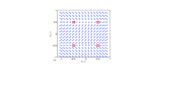
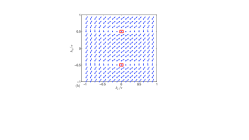
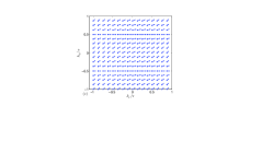
Figure 3: The vortex structure of the EPs in $\boldsymbol{k}$ plane, described by the field distribution based on the Eq. (20) with $N=M=16$. The parameter choices are (a)$\gamma=\sqrt{3},\delta=1/\sqrt{2}$ in the area EPs exist; (b)$\gamma=2,\delta=1/\sqrt{2}$ in the phase boundary; (c)$\gamma=0,\delta=1/\sqrt{2}$ in the unbroken real energy area, with the unit of $J$. The red square in (a) and (b) show the position of EPs. Those figures correspond with the three situations we mentioned before.

Also, if we consider the open boundary condition in the $y$ direction when $M$ is odd and keep other conditions as same as before, the only change would be $k_{y}\rightarrow\frac{\pi n}{M+1}.$For $n=(M+1)/2,$ there are still two EPs with topological features, as the projection from the $2$D thermodynamic limit.

IV Single-chain situation

The above analysis is for the $2$D system. However, we note that the position of EPs is only restricted to $k_{cy}=\pm\pi/2$. A straightforward derivation is that the topological feature of EP in the $2$D system can be retrieved from coupled-chain or quasi-$1$D system. Based on this idea, we consider $M=1$, i.e., a single-chain Hamiltonian below

$$H = -J\sum_{l=1}^{2N}\left[1+\left(-1\right)^{l}\delta\right]\left(c_{l}^{\dagger}c_{l+1}+\mathrm{H.c.}\right)$$

$$+i\gamma\sum_{l}\left(-1\right)^{l}c_{l}^{\dagger}c_{l},$$

with the periodic boundary condition. Here, without loss of generality, we define the action of time-reversal and parity in such a ring system as follows. While the time-reversal operation $\mathcal{T}$ is defined as $\mathcal{T}i\mathcal{T}=-i$, the effect of the parity is $\mathcal{P}c_{l}^{\dagger}\mathcal{P}=c_{2N+1-l}^{\dagger}$.

In fact, it can be seen as a SSH chain system, in which the hopping amplitudes of the chain is staggered. Fig. 1 sketches the geometry of the system. Following the same step we did in Sec. II, it is quite easy to find the core matrix of $H=\sum_{\boldsymbol{k}}H_{\boldsymbol{k}}$ is

$$h_{k}=-J\left(\begin{array}[]{cc}i\frac{\gamma}{J}&w+ve^{-ik}\\ w+ve^{ik}&-i\frac{\gamma}{J}\end{array}\right),$$ (26)

where $w=1-\delta$, $v=1+\delta$ and the wave vector $k=2\pi n/N-\pi$, $(n=0,1,...,N-1)$. The phase boundary can be obtained by the zero points of the spectrum

$$\varepsilon_{k} = \pm J\sqrt{4wv\cos^{2}\left(\frac{k}{2}\right)+\left(w-v\right)^{2}-\left(\frac{\gamma}{J}\right)^{2}}$$ (27)

$$= \pm 2J\sqrt{\left(1-\delta^{2}\right)\cos^{2}\left(\frac{k}{2}\right)+\delta^{2}-\left(\frac{\gamma}{2J}\right)^{2}},$$

with the eigenvector

$$\left|\psi_{k}^{\pm}\right\rangle=\frac{1}{\sqrt{\Delta}}\left(\begin{array}[]{c}\frac{1}{J\left(w+ve^{ik}\right)}\left(i\gamma\mp\varepsilon_{k}\right)\\ 1\end{array}\right),$$ (28)

which are normalized by the Dirac normalization factor

$$\Delta=\frac{\varepsilon_{k}^{2}+\left|\varepsilon_{k}\right|^{2}\mp 2\gamma\mathrm{Im}\varepsilon_{k}+2\gamma^{2}}{\varepsilon_{k}^{2}+\gamma^{2}}.$$ (29)

From $\varepsilon_{k}=0$, we have equations

$$\left(1-\delta^{2}\right)\cos^{2}\left(\frac{k}{2}\right)+\delta^{2}-\left(\frac{\gamma}{2J}\right)^{2}=0.$$ (30)

It is obvious that the phase diagram of this single-chain model is as same as what is shown in Fig. 2. In Fig. 4, we provide more details about the energy band structure of different parameters which are marked in Fig. 2, the numerical result accords with the analysis above.

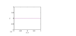
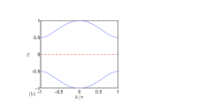
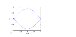
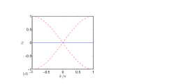
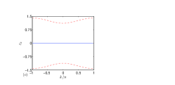
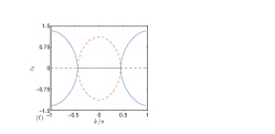
Figure 4: (Color online) Plots of the structure of the energy band described by Eq. (27) at some points fixed in Fig. 2. The blue line means the real part of $\pm\varepsilon_{k}$, the red dashed line means the imaginary part of $\pm\varepsilon_{k}$, respectively. $J=1/2$ for all figures. Graphs (a), (c), (d), and (f) show the energy band situation in the nontrivial area where the EPs exist. Meanwhile (b) and (e) display the situation in the trivial area where $\varepsilon_{k}$ is always non-zero.

The $2$D vector field $F(k)$ is still effective and reduces to $F(k)$, which displays the topological property as the kink for $k$ in $1$D, as shown along $k_{x}$ direction with $k_{y}=\pm\pi/2$ in Fig. 3(a). A pair of kinks will meet with each other at the phase boundary, and disappear as the parameters reach the unbroken area, which is the same as the $2$D system result.

V Symmetry protection of kinks

As we mentioned in the introduction, the kink represented by $F(k)$ in the single-chain system is a topological invariant, which is protected by the symmetry of the Hamiltonian. To see this point, we firstly introduce the eigenstate of the $h_{k}$

$$\left|\varphi_{k}^{\pm}\right\rangle = \frac{1}{\sqrt{\Omega}}\left(\begin{array}[]{c}\frac{1}{J\left(w+ve^{ik}\right)}\left(i\gamma\mp\varepsilon_{k}\right)\\ 1\end{array}\right),$$ (33)

$$\left|\phi_{k}^{\pm}\right\rangle = \frac{1}{\sqrt{\Omega^{\ast}}}\left(\begin{array}[]{c}\frac{1}{J\left(w+ve^{ik}\right)}\left(-i\gamma\mp\varepsilon_{k}^{\ast}\right)\\ 1\end{array}\right),$$ (36)

which are normalized by the biorthogonal normalization with

$$\Omega=\frac{2\varepsilon_{k}\left(\varepsilon_{k}+i\gamma\right)}{\varepsilon_{k}^{2}+\gamma^{2}},$$ (37)

and satisfy

$$\left\langle\phi_{k}^{a}\right|\varphi_{k}^{b}\rangle = \delta_{a,b},\varepsilon_{k}^{2}>0,$$

$$\left\langle\phi_{k}^{a}\right|\varphi_{k}^{b}\rangle = \delta_{a,-b},\varepsilon_{k}^{2}<0.$$ (38)

Then we define

$$Q_{x}=\sigma_{x}\mathcal{T}.$$ (39)

This operator can be seen as a combination of the inversion operator $\mathcal{P}$ and time-reversal operator $\mathcal{T}$, and leads to $\left[Q_{x},h_{k}\right]=0$. So

$$Q_{x}\left|\varphi_{k}^{-}\right\rangle=\frac{1}{\sqrt{\Omega^{\ast}}}\frac{-i\gamma+\varepsilon_{k}^{\ast}}{J\left(w+ve^{-ik}\right)}\left(\begin{array}[]{c}\frac{1}{J\left(w+ve^{ik}\right)}\left(i\gamma+\varepsilon_{k}^{\ast}\right)\\ 1\end{array}\right)$$ (40)

is still a eigenstate of $h_{k}$. When $\varepsilon_{k}^{2}>0$

$$Q_{x}\left|\varphi_{k}^{-}\right\rangle=\sqrt{\frac{w+ve^{ik}}{w+ve^{-ik}}}\left|\varphi_{k}^{-}\right\rangle,$$ (41)

when $\varepsilon_{k}^{2}<0$

$$Q_{x}\left|\varphi_{k}^{-}\right\rangle=-\frac{i\gamma+\varepsilon_{k}}{J\left(w+ve^{-ik}\right)}\left|\varphi_{k}^{+}\right\rangle,$$ (42)

the symmetry breaking happens. According to the above conclusion, a straightforward calculation of $\left|\left\langle Q_{x}^{\mathrm{B}}\right\rangle_{k}\right|=\left|\left\langle\phi_{k}^{-}\right|Q_{x}\left|\varphi_{k}^{-}\right\rangle\right|$ shows that

$$\left|\left\langle Q_{x}^{\mathrm{B}}\right\rangle_{k}\right|=\left\{\begin{array}[]{c}1,\varepsilon_{k}\text{ is real}\\ 0,\varepsilon_{k}\text{ is imagine}\end{array}\right.,$$ (43)

which indicates the topological property of the EP as a critical point of values $0$ and $1$ in the basis of the biorthogonal eigenvectors.

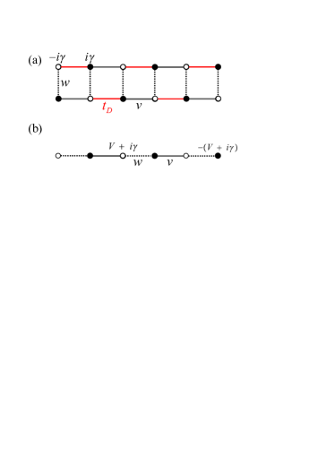
Figure 5: (Color online) Schematics of two kinds of perturbation on the SSH chain at EPs. (a)Extra hopping term (red line) with amplitude $t_{\mathrm{D}}$. (b)Staggered on-site real potentials on two sublattices indicated by filled and empty circles, respectively. In the case of (a), the topology of EPs is an invariant under the perturbations, while the EPs is eliminated for non-zero $V$ in the case (b).

VI Perturbations

In a Hermitian system, the topological invariant for the topological boundary is essentially the topologically unavoidable band touching points Li2 ; SCZ . For a non-Hermitian one, as we proved before, it is the topological unavoidable EPs. Once the parameters of the system change within some particular areas, the EPs always exist. This topological feature may be robust for some kinds of perturbation but fragile for others. We consider two kinds of perturbations, with an extra hopping across the neighboring site and staggered on-site real potential, respectively. Fig. 5 sketches the structures of these two cases. We will focus on the effects of the extra terms on the existence of the EPs.

For the first case, the Hamiltonian can be written as

$$H_{\mathrm{D}}=H-Jt_{\mathrm{D}}\sum_{l=1}^{N}(a_{l}^{\dagger}b_{l+1}+\mathrm{H.c.}),$$ (44)

where $t_{\mathrm{D}}$ denotes the extra hopping amplitude. Based on the Fourier transformations, we still have

$$H_{\mathrm{D}}=\sum_{k}(a_{k}^{\dagger},b_{k}^{\dagger})h_{k}^{\mathrm{D}}\left(\begin{array}[]{c}a_{k}\\ b_{k}\end{array}\right),$$ (45)

and

$$h_{k}^{\mathrm{D}}=h_{k}-Jt_{\mathrm{D}}\left(\begin{array}[]{cc}0&e^{-ik}\\ e^{ik}&0\end{array}\right).$$ (46)

The spectrum is

$$\varepsilon_{k}^{\mathrm{D}}=\pm J\sqrt{4w\left(v+t_{\mathrm{D}}\right)\cos^{2}\left(\frac{k}{2}\right)+\left[w-\left(v+t_{\mathrm{D}}\right)\right]^{2}-\left(\frac{\gamma}{J}\right)^{2}},$$ (47)

which only has a shift on $v$, i.e., $v\rightarrow v+t_{\mathrm{D}}$, from the spectrum $\varepsilon_{k}$ in Eq. (27). Thus the zero energy point can be obtained directly as following. There are still three types of zero energy points. (I) $\delta=1$ or $-\left(1+t_{\mathrm{D}}\right),\frac{\gamma}{2J}=\pm\left(1+\frac{t_{\mathrm{D}}}{2}\right)$. (II) $k_{c}=\pm\pi,\delta=\pm\frac{\gamma}{2J}-\frac{t_{\mathrm{D}}}{2}$ or $k_{c}=0,\frac{\gamma}{2J}=\pm\left(1+\frac{t_{\mathrm{D}}}{2}\right)$. (III) When $\gamma$ and $\delta$ are in the area

$$\frac{\gamma}{2J} \in \left(-\left|1+\frac{t_{\mathrm{D}}}{2}\right|,\left|1+\frac{t_{\mathrm{D}}}{2}\right|\right),$$

$$\delta \in \left(-\left|\frac{\gamma}{2J}\right|-\frac{t_{\mathrm{D}}}{2},\left|\frac{\gamma}{2J}\right|-\frac{t_{\mathrm{D}}}{2}\right),$$ (48)

or

$$\frac{\gamma}{2J} \in \left(-\infty,-\left|1+\frac{t_{\mathrm{D}}}{2}\right|\right)\cup\left(\left|1+\frac{t_{\mathrm{D}}}{2}\right|,+\infty\right),$$ (49)

$$\delta \in \left(-\infty,\left|\frac{\gamma}{2J}\right|-\frac{t_{\mathrm{D}}}{2}\right)\cup\left(\left|\frac{\gamma}{2J}\right|-\frac{t_{\mathrm{D}}}{2},+\infty\right),$$

there are always two values of $k$: $\pm k_{c},k_{c}\in\left(0,\pi\right)$, which satisfy

$$\frac{\left(\frac{\gamma}{2J}\right)^{2}-\left(\delta+\frac{t_{\mathrm{D}}}{2}\right)^{2}}{\left(1-\delta\right)\left(1+\delta+t_{\mathrm{D}}\right)}=\cos^{2}\left(\frac{k_{c}}{2}\right).$$ (50)

It is clear that for small $t_{\mathrm{D}}$, the phase diagram changes a little comparing to the case with zero $t_{\mathrm{D}}$, but keep the original geometry, which means the Hamiltonian still satisfies $\left[Q_{x},h_{k}^{\mathrm{D}}\right]=0$. The position of the EP, $k_{c}$, shifts a little without changing the original topology, i.e., the topological charge of the kink. Then the EP is a topological invariant under the perturbation from the $t_{\mathrm{D}}$ term.

For the second case, the Hamiltonian can be written as

$$H_{\mathrm{V}}=H+V\sum_{j=1}^{N}(b_{j}^{\dagger}b_{j}-a_{j}^{\dagger}a_{j})\mathrm{,}$$ (51)

which indicates that particles on different sub-lattices have opposite real chemical potentials. The extra potentials do not break the translational symmetry. By the same procedure, we have

$$H_{\mathrm{V}}=\sum_{k}(a_{k}^{\dagger},b_{k}^{\dagger})h_{k}^{\mathrm{v}}\left(\begin{array}[]{c}a_{k}\\ b_{k}\end{array}\right),$$ (52)

and

$$h_{k}^{\mathrm{v}}=-J\left(\begin{array}[]{cc}\frac{V+i\gamma}{J}&w+ve^{-ik}\\ w+ve^{ik}&-\frac{V+i\gamma}{J}\end{array}\right).$$ (53)

The spectrum is

$$\varepsilon_{k}^{\mathrm{v}} = \pm J\sqrt{4wv\cos^{2}\left(\frac{k}{2}\right)+\left(w-v\right)^{2}+\left(\frac{V+i\gamma}{J}\right)^{2}}$$ (54)

$$= \pm 2J\sqrt{\left(1-\delta^{2}\right)\cos^{2}\left(\frac{k}{2}\right)+\delta^{2}+\left(\frac{V+i\gamma}{2J}\right)^{2}},$$

which clearly shows that the nonzero $V$ can let the energy be complex with $\gamma\neq 0$, i.e., no real energy exist, and destroy the topological EPs. This can be associated with the inversion symmetry $\mathcal{P}$ broken, which leads to $\left[Q_{x},h_{k}^{\mathrm{V}}\right]\neq 0$, leave the EP without the symmetry protection.

VII Summary

In this paper, we study $M$ coupled non-Hermitian Rice-Mele chains with length $2N$. The EPs appeared in this model can be two isolated points in $2$D $\boldsymbol{k}$-plane for infinite $M$ and $N$ or $2$D thermodynamic limit. It is shown that two isolated EPs are topological defects of an auxiliary field achieved by mapping the the Bloch states of the model onto a $2$D real vector field in $\boldsymbol{k}$-plane, with topological charge $\pm 1/2$. Furthermore, we extend this analysis to finite $M$ cases with periodic and open boundary conditions and find that the auxiliary field on the discrete $\boldsymbol{k}$-space for finite $M$ is the projection of the infinite one for the $2$D model. It is shown that the EPs in finite $M$ systems still possess topological features. Besides, we focus on the single chain system and find that two topological defects in $2$D $\boldsymbol{k}$ space reduce to a pair of kinks in $1$D $k$ space. The corresponding topological invariant is protected by the combined inversion and time-reversal symmetry. At last, we show the robust topological feature of the EPs in non-Hermitian systems is as same as the band touching points in Hermitian systems.

Since it proves that the topological invariants for a quasi-$1$D system can be extracted from the projection of the corresponding $2$D limit system on it, and the topological feature for some quasi-$1$D systems is not easy to describe due to there is only one variable in $\boldsymbol{k}$ space. This work also provides an alternative way to capture the topological feature in the quasi-$1$D system by exploring the $2$D expansion of the original system.

- (1) C. M. Bender and S. Boettcher, Phys. Rev. Lett. 80, 5243 (1998); C. M. Bender, D. C. Brody, H. F. Jones, Phys. Rev. Lett. 89, 270401 (2002); Phys. Rev. Lett. 98, 040403 (2007); C. M. Bender, D. W. Hook, P. N. Meisinger, and Q. H. Wang, Phys. Rev. Lett. 104, 061601 (2010).
- (2) S. Longhi, Phys. Rev. Lett. 105, 013903 (2010);
- (3) C. T. West, T. Kottos, and T. Prosen, Phys. Rev. Lett. 104, 054102 (2010).
- (4) C. Li and Z. Song, Phys. Rev. A 91, 062104 (2015); C. Li, L. Jin, and Z. Song, Phys. Rev. A 95, 022125 (2017).
- (5) W. J. Chen, Ş. K. Özdemir, G. M. Zhao, J. Wiersig, and L. Yang, Nature 548, 192-196 (2017).
- (6) J. Zhang, et al., Nat. Photon. 12, 479–484 (2018).
- (7) S. Longhi, Opt. Lett. 43, 2929 (2018).
- (8) T. Goldzak, A. A. Mailybaev, and N. Moiseyev, Phys. Rev. Lett. 120, 013901 (2018).
- (9) C. H. Yi, J. Kullig, and J. Wiersig, Phys. Rev. Lett. 120, 093902 (2018).
- (10) W. D. Heiss, J. Phys. A: Math. Theor. 45, 444016 (2012).
- (11) A. Mostafazadeh, J. Math. Phys. 43, 205-214 (2002); J. Phys. A: Math. Gen. 36, 7081-7091 (2003); J. Phys. A: Math. Gen. 37, 11645-11679 (2004).
- (12) A. Mostafazadeh and H. J. Mehri-Dehnavi, Phys. A: Math. Theor. 42, 125303 (2009); A. Mostafazadeh, Phys. Rev. Lett. 102, 220402 (2009); Phys. Rev. A 80, 032711 (2009); J. Phys. A: Math. Theor. 44, 375302 (2011); A. Mostafazadeh and M. Sarisaman, Phys. Lett. A 375, 3387-3391 (2011).
- (13) K. Esaki, M. Sato, K. Hasebe, and M. Kohmoto, Phys. Rev. B 84, 205128 (2011).
- (14) T. E. Lee, Phys. Rev. Lett. 116, 133903 (2016).
- (15) C. Li, G. Zhang, and Z. Song, Phys. Rev. A 94, 052113 (2016); C. Li, X. Z. Zhang, G. Zhang, and Z. Song, Phys. Rev. B 97, 115436 (2018).
- (16) S. Lin, G. Zhang, and Z. Song, Sci. Rep 6, 31953 (2016).
- (17) D. Leykam, K. Y. Bliokh, C. L. Huang, Y. D. Chong, and F. Nori, Phys. Rev. Lett. 118, 040401 (2017).
- (18) H. T. Shen, B. Zhen, and L. Fu, Phys. Rev. Lett. 120, 146402 (2018).
- (19) S. Y. Yao and Z. Wang, Phys. Rev. Lett. 121, 086803 (2018).
- (20) Z. Gong, Y. Ashida, K. Kawabata, K. Takasan, S. Higashikawa, and M. Ueda, Phys. Rev. X 8, 031079 (2018).
- (21) K. Ding, G. C. Ma, M. Xiao, Z. Q. Zhang, and C. T. Chan, Phys. Rev. X 6, 021007 (2016).
- (22) J. Dopple, et al. Nature 537, 76–79 (2016).
- (23) S. Weimann, et al. Nat. Mat. 16, 433–438 (2016).
- (24) B. Midya, H. Zhao, and L. Feng, Nat. Commun. 9, 2674 (2018).
- (25) D. Xiao, M. C. Chang, and Q. Niu, Rev. Mod. Phys. 82, 1959 (2010)
- (26) M. Z. Hasan and C. L. Kane, Rev. Mod. Phys. 82, 3045 (2010).
- (27) X. L. Qi and S. C. Zhang, Rev. Mod. Phys. 83, 1057 (2011).
- (28) A. A. Burkov and L. Balents, Phys. Rev. Lett. 107, 127205 (2011).
- (29) G. Xu, H. Weng, Z. Wang, X. Dai, and Z. Fang, Phys. Rev. Lett. 107, 186806 (2011).
- (30) S. M. Young, S. Zaheer, J. C. Y. Teo, C. L. Kane, E. J. Mele, and A. M. Rappe, Phys. Rev. Lett. 108, 140405 (2012).
- (31) K. Sun, W. V. Liu, A. Hemmerich, and D. Sama, Nature. Phys. 8, 67–70 (2012).
- (32) H. Weng, C. Fang, Z. Fang, B. A. Bernevig, and X. Dai, Phys. Rev. X 5, 011029 (2015).
- (33) S. M. Huang, et al. Nat. Commun. 6, 7373 (2015).
- (34) J. M. Hou, Phys. Rev. Lett. 111, 130403 (2013).
- (35) Z. K. Liu, et al. Science 343, 864–867 (2014).
- (36) M. Neupane, et al. Nat. Commun. 5, 3786 (2014).
- (37) S. Y. Xu, et al. Science 349, 613–617 (2015).
- (38) B. Q. Lv, et al. Phys. Rev. X 5, 031013 (2015).
- (39) L. Lu, et al. Science 349, 622–624 (2015).
- (40) M. J. Rice and E. J. Mele, Phys. Rev. Lett. 49, 1455 (1982).
- (41) S. Lin, X. Z. Zhang, and Z. Song, Phys, Rev. A 92, 012117 (2015).
- (42) R. Wang, X. Z. Zhang, and Z. Song, Phys. Rev. A 98, 042120 (2018).
- (43) W. P. Su, J. R. Schrieffer, and A. J. Heeger, Phys. Rev. B 22, 2099 (1980).
- (44) J. K. Asbóth, L. Oroszlány, and A. Pályi, A Short Course on Topological Insulators, Lecture Notes in Physics 919 (Springer International Publishing, Switzerland, 2016).
- (45) J. C. Y. Teo and C. L. Kane, Phys. Rev. B 82, 115120 (2010).
- (46) Y. Q. Yan and Q. Zhou, Phys. Rev. Lett. 120, 235302 (2018).
- (47) C. Li, S. Lin, G. Zhang, and Z. Song, Phys. Rev. B 96, 125418 (2017).
- (48) J. Wang and S. C. Zhang, Nat. Mater. 16, 1062-1067 (2017).